I do not pretend to start with precise questions. I do not think youcan start with anything precise. You have to achieve such preci-sion as you can, as you go along.

—Bertrand Russell, The Philosophy of Logical Atomism (1918)

Chapter 7

Sparse interpolation

The next two chapters examine methods to determine the sparse representation of anunknown polynomial, given only a way to evaluate the polynomial at chosen points. Thesemethods are generally termed black-box sparse interpolation.

First, we examine a new approach to the standard sparse interpolation problem over largefinite fields and approximate complex numbers. This builds on recent work by Garg andSchost (2009), improving the complexity of the fastest existing algorithm over large finitefields, and the numerical stability of the state of the art for approximate sparse interpola-tion. The primary new tool that we introduce is a randomised method to distinguish termsin the unknown polynomial based on their coefficients, which we term diversification. Us-ing this technique, our new algorithms gain practical and theoretical efficiency over previousmethods by avoiding the need to use factorization algorithms as a subroutine.

We gratefully acknowledge the helpful and useful comments by Éric Schost as well as theSymbolic Computation Group members at the University of Waterloo on preliminary versionsof the work in this chapter.

7.1 Background

Polynomial interpolation is a long-studied and important problem in computer algebra andsymbolic computation. Given a way to evaluate an unknown polynomial at any chosen point,and an upper bound on the degree, the interpolation problem is to determine a representa-tion for the polynomial. In sparse interpolation, we are also given an upper bound on thenumber of nonzero terms in the unknown polynomial, and the output is returned in thesparse representation. Generally speaking, we seek algorithms whose cost is polynomially-bounded by the size of the output, i.e., the sparse representation size of the unknown polyno-mial.

117

CHAPTER 7. SPARSE INTERPOLATION

Sparse interpolation has numerous applications in computer algebra and engineering.Numerous mathematical computations suffer from the problem of intermediate expressionswell, whereby the size of polynomials encountered in the middle of a computation is muchlarger than the size of the input or the output. In such cases where the output is known tobe sparse, sparse interpolation can eliminate the need to store large intermediate expressionsexplicitly, thus greatly reducing not only the intermediate storage requirement but also thecomputational cost. Important examples of such problems are multivariate polynomial fac-torization and system solving (Canny, Kaltofen, and Yagati, 1989; Kaltofen and Trager, 1990;Díaz and Kaltofen, 1995, 1998; Javadi and Monagan, 2007, 2009).

Solving non-linear systems of multivariate polynomials with approximate coefficients hasnumerous practical applications, especially in engineering (see for example Sommese andWampler, 2005). Homotopy methods are a popular way of solving such systems and relatedproblems by following the paths of single solution points from an initial, easy system, to thetarget system of interest. Once enough points are known in the target system, sparse inter-polation methods are used to recover a polynomial expression for the actual solution. Thesetechniques generally fall under the category of hybrid symbolic-numeric computing, and inparticular have been applied to solving non-linear systems (e.g., Sommese, Verschelde, andWampler, 2001, 2004; Stetter, 2004) and factoring approximate multivariate polynomials (e.g.,Kaltofen, May, Yang, and Zhi, 2008).

Sparse interpolation is also of interest in theoretical computer science. It is a non-trivialgeneralisation of the important problem of polynomial identity testing, or PIT for short. Gen-erally speaking, the PIT problem is to identify whether the polynomial represented by a givenalgebraic circuit is identically zero. Surprisingly, although this question is easily answeredusing randomisation and the classical results of Demillo and Lipton (1978); Zippel (1979);Schwartz (1980), no deterministic polynomial-time algorithm is known. In fact, even de-randomising the problem for circuits of depth four would have important consequences (Ka-banets and Impagliazzo, 2004). We will not discuss this problem further, but the point thereader to the excellent recent surveys of Saxena (2009) and Shpilka and Yehudayoff (2010).

7.1.1 Problem definition

Let f ∈ F[x1, . . . ,xn ] have degree less than d . A black box for f is a function which takes asinput a vector (a 1, . . . , a n ) ∈ Fn and produces f (a 1, . . . , a n ) ∈ F. The cost of the black box is thenumber of operations in F required to evaluate it at a given input.

Clausen, Dress, Grabmeier, and Karpinski (1991) showed that, if only evaluations over theground field F are allowed, then for some instances at least Ω(n log t ) black box probes are re-quired. Hence if we seek polynomial-time algorithms, we must extend the capabilities of theblack box. To this end, Díaz and Kaltofen (1998) introduced the idea of an extended domainblack box which is capable of evaluating f (b1, . . . ,bn ) ∈ E for any (b1, . . . ,bn ) ∈ En where E isany extension field of F . That is, we can change every operation in the black box to work overan extension field, usually paying an extra cost per evaluation proportional to the size of theextension.

118

CHAPTER 7. SPARSE INTERPOLATION

Motivated by the case of black boxes that are division-free algebraic circuits, we will usethe following model which we believe to be fair and cover all previous relevant results. Againwe use the notation of M(m ) for the number of field operations required to multiply twodense univariate polynomials with degrees less than m , and O (m ) to represent any functionbounded by m (log m )O(1).

Definition 7.1. Let f ∈ F[x1, . . . ,xn ] and ` > 0. A remainder black box for f with size ` is aprocedure which, given any monic square-free polynomial g ∈ F[y ] with deg g =m , and anyh1, . . . , hn ∈ F[y ] with each deg h i < m , produces f (h1, . . . , hn )rem g using at most ` ·M(m )operations in F.

This definition is general enough to cover the algorithms we know of over finite fields, andwe submit that the cost model is fair to the standard black box, extended domain black box,and algebraic circuit settings. The model also makes sense over complex numbers, as we willsee.

7.1.2 Interpolation over finite fields

We first summarize previously known univariate interpolation algorithms when F is a finitefield with q elements and identify our new contributions here. For now, let f ∈ Fq [x ] havedegree less than d and sparsity t . We will assume we have a remainder black box for f withsize `. Since field elements can be represented with O(logq ) bits, a polynomial-time algorithmwill have cost polynomial in `, t , log d , and logq .

For the dense output representation, one can use the classical method of Newton, Waring,and Lagrange to interpolate in O (`d ) time (von zur Gathen and Gerhard, 2003, §10.2).

The algorithm of Ben-Or and Tiwari (1988) for sparse polynomial interpolation, and inparticular the version developed by Kaltofen and Yagati (1989), can be adapted to arbitraryfinite fields. Unfortunately, these algorithms require t discrete logarithm computations in F∗q ,whose cost is small if the field size q is chosen carefully (as in Kaltofen (2010)), but not ingeneral. For arbitrary (and potentially large) q , we can take advantage of the fact that eachdiscrete logarithm that needs to be computed falls in the range [0, 1, . . . , d −1]. The “kangaroomethod” of Pollard (1978, 2000) can, with high probability, compute such a discrete log withO(p

d ) field operations. Using this algorithm makes brings the total worst-case cost of Ben-Orand Tiwari’s algorithm to O(t `+ t 2+ t

pd ).

This chapter builds most directly on the work of (Garg and Schost, 2009), who gave thefirst polynomial-time algorithm for sparse interpolation over an arbitrary finite field. Theiralgorithm works roughly as follows. For very small primes p , use the black box to compute fmodulo x p − 1. A prime p is a “good prime” if and only if all the terms of f are still distinctmodulo x p − 1. If we do this for all p in the range of roughly O(t 2 log d ), then there will besufficient good primes to recover the unique symmetric polynomial over Z[y ] whose rootsare the exponents of nonzero terms in f . We then factor this polynomial to find those expo-nents, and correlate with any good prime image to determine the coefficients. The total costis O (`t 4 log2 d )field operations. Using randomization, it is easy to reduce this to O (`t 3 log2 d ).

119

CHAPTER 7. SPARSE INTERPOLATION

Probes Probe degree Computation cost Total costDense d 1 O (d ) O (`d )

Ben-Or & Tiwari O(t ) 1 O(t 2+ tp

d ) O (`t + t 2+ tp

d )Garg & Schost O (t 2 log d ) O (t 2 log d ) O (t 4 log2 d ) O (`t 4 log2 d )

Randomized G & S O (t log d ) O (t 2 log d ) O (t 3 log2 d ) O (`t 3 log2 d )Ours O(log d ) O (t 2 log d ) O (t 2 log2 d ) O (`t 2 log2 d )

Table 7.1: Sparse univariate interpolation over large finite fields,with black box size `, degree d , and t nonzero terms

Observe that the coefficients of the symmetric integer polynomial in Garg & Schost’s al-gorithm are bounded by O(d t ), which is much larger than the O(d ) size of the exponentsultimately recovered. Our primary contribution over finite fields of size at least Ω(t 2d ) is anew algorithm which avoids evaluating the symmetric polynomial and performing root find-ing over Z[y ]. As a result, we reduce the total number of required evaluations and developa randomized algorithm with cost O (`t 2 log2 d ), which is roughly quadratic in the input andoutput sizes. Since this can be deterministically verified in the same time, our algorithm (aswell as the randomized version of Garg & Schost) is of the Las Vegas type.

The relevant previous results mentioned above are summarized in Table 7.1, where weassume in all cases that the field size q is “large enough”. In the table, the “probe degree”refers to the degree of g in each evaluation of the remainder black box as defined above.

7.1.3 Multivariate interpolation

Any of the univariate algorithms above can be used to generate a multivariate polynomialinterpolation algorithm in at least two different ways. For what follows, write ρ(d , t ) for thenumber of remainder black box evaluations required by some univariate interpolation algo-rithm,∆(d , t ) for the degree of the remainder in each evaluation, andψ(d , t ) for the numberof other field operations required besides black box calls. Observe that these correspond tothe first three columns in Table 7.1.

The first way to adapt a univariate interpolation algorithm to a multivariate one is Kro-necker substitution: given a remainder black box for an unknown f ∈ F[x1, . . . ,xn ], with eachpartial degree less than d , we can easily construct a remainder black box for the univariatepolynomial f = f (x ,x d ,x d 2 , . . . ,x d n−1) ∈ F[x ], whose terms correspond one-to-one with termsof f . This is the approach taken for instance in Kaltofen (2010, §2) for the interpolation ofmultivariate polynomials with rational coefficients. The cost is simply the cost of the chosenunderlying univariate algorithm, with the degree increased to d n .

The other method for constructing a multivariate interpolation algorithm is due to Zip-pel (1990). The technique is inherently probabilistic and works variable-by-variable, at eachstep solving a number of t × t transposed Vandermonde systems, for some t ≤ t . Specifically,each system is of the form Ax = b , where A is a t × t matrix of scalars from the coefficientfield Fq . The vector v consists of the output of t remainder black box evaluations, and so its

120

CHAPTER 7. SPARSE INTERPOLATION

Kronecker ZippelDense O (`d n ) O (`nt d )

Ben-Or & Tiwari O (`t + t 2+ t d n/2) O (nt 3+nt 2p

d + `nt 2)Garg & Schost O (`n 2t 4 log2 d ) O (`nt 5 log2 d )

Randomized G & S O (`n 2t 3 log2 d ) O (`nt 4 log2 d )Ours O (`n 2t 2 log2 d ) O (`nt 3 log2 d )

Table 7.2: Sparse multivariate interpolation over large finite fields,with black box size `, n variables, degree d , and t nonzero terms

elements are in Fq [y ], and the system must be solved modulo some g ∈ Fq [y ], as specifiedby the underlying univariate algorithm. Observe however that since A does not contain poly-nomials, computing x = A−1b requires no modular polynomial arithmetic. In fact, using thesame techniques as Kaltofen and Yagati (1989, §5), employing fast dense bivariate polynomialarithmetic, each system can be solved using

O

M

t ·∆(d , t )

· log

t ·∆(d , t )

field operations.

Each transposed Vandermonde system gives the remainder black box evaluation of eachof t univariate polynomials that we are interpolating in that step. The number of such systemsthat must be solved is thereforeρ(d , t ), as determined by the underlying univariate algorithm.Finally, each of the t univariate interpolations proceeds with the given evaluations. The totalcost, over all iterations, is

O˜

`nt ·∆(d , t ) ·ρ(d , t )

field operations for the remainder black box evaluations, plus

O˜

ntψ(d , t )+ `nt ·∆(d , t )

field operations for additional computation. Zippel (1990) used the dense algorithm for uni-variate interpolation; using Ben-Or and Tiwari’s algorithm instead was studied by Kaltofenand Lee (2003).

Table 7.2 summarizes the cost of the univariate algorithms mentioned above applied tosparse multivariate interpolation over a sufficiently large finite field, using Kronecker’s andZippel’s methods.

For completeness, we mention a few more results on closely related problems that do nothave a direct bearing on the current study. Grigoriev, Karpinski, and Singer (1990) give a par-allel algorithm with small depth but which is not competitive in our model due to the largenumber of processors required. A practical parallel version of Ben-Or and Tiwari’s algorithmhas been developed by (Javadi and Monagan, 2010). (Kaltofen, Lakshman, and Wiley, 1990)and (Avendaño, Krick, and Pacetti, 2006) present modular algorithms for interpolating poly-nomials with rational and integer coefficients. However, their methods do not seem to applyto finite fields.

121

CHAPTER 7. SPARSE INTERPOLATION

7.1.4 Approximate Polynomial Interpolation

In Section 7.4 we consider the case of approximate sparse interpolation. Our goal is to pro-vide both a numerically more robust practical algorithm, but also the first algorithm which isprovably numerically stable, with no heuristics or conjectures. We define an “ε-approximateblack box” as one which evaluates an unknown t -sparse target polynomial f ∈ C[x ], of de-gree d , with relative error at most ε > 0. Our goal is to build a t -sparse polynomial g suchthat

f − g

≤ ε

f

. A bound on the degree and sparsity of the target polynomial, as well asε, must also be provided. In Section 7.4 we formally define the above problem, and demon-strate that the problem of sparse interpolation is well-posed. We then adapt our variant ofthe (Garg and Schost, 2009) algorithm for the approximate case, prove it is numerically accu-rate in terms of the relative error of the output, and analyze its cost. We also present a fullimplementation in Section 7.5 and validating experiments.

Recently, a number of numerically-focussed sparse interpolation algorithms have beenpresented. The algorithm of (Giesbrecht, Labahn, and Lee, 2009) is a numerical adaptationof (Ben-Or and Tiwari, 1988), which samples f at O(t ) randomly chosen roots of unityω ∈Con the unit circle. In particular, ω is chosen to have (high) order at least the degree, anda randomization scheme is used to avoid clustering of nodes which will cause dramatic ill-conditioning. A relatively weak theoretical bound is proven there on the randomized condi-tioning scheme, though experimental and heuristic evidence suggests it is much better inpractice. (Cuyt and Lee, 2008) adapt Rutishauser’s qd algorithm to alleviate the need forbounds on the partial degrees and the sparsity, but still evaluate at high-order roots of unity.Approximate sparse rational function interpolation is considered by (Kaltofen and Yang, 2007)and (Kaltofen, Yang, and Zhi, 2007), using the Structured Total Least Norm (STLN) methodand, in the latter, randomization to improve conditioning. Approximate sparse interpolationis also considered for integer polynomials by (Mansour, 1995), where a polynomial-time al-gorithm is presented in quite a different model from ours. In particular the evaluation erroris absolute (not relative) and the complexity is sensitive to the bit length of the integer coeffi-cients.

Note that all these works evaluate the polynomial only on the unit circle. This is necessarybecause we allow and expect f to have very large degree, which would cause a catastrophicloss of precision at data points of non-unit magnitude. Similarly, we assume that the complexargument of evaluation points is exactly specified, which is again necessary because any errorin the argument would be exponentially magnified by the degree.

The primary contribution of our work in Section 7.4 below is to provide an algorithm withboth rigorously provable relative error and good practical performance. Our algorithm typi-cally requires O (t 2 log2 d ) evaluations at primitive roots of unity of order O (t 2 log d ) (as op-posed to order d in previous approaches). We guarantee that it finds a t -sparse polynomialg such that

g − f

≤ 2ε

f

. An experimental demonstration of the numerical robustness isgiven in Section 7.5.

122

CHAPTER 7. SPARSE INTERPOLATION

7.2 Sparse interpolation for generic fields

For the remainder, we assume the unknown polynomial f is always univariate. This is with-out loss of generality, as we can use the Kronecker substitution as discussed previously. Theexponential increase in the univariate degree only corresponds to a factor of n increase inlog deg f , and since our algorithms will ultimately have cost polynomial in log deg f , polyno-mial time is preserved.

Assume a fixed, unknown, t -sparse univariate polynomial f ∈ F[x ]with degree at most d .We will use a remainder black box for f to evaluate f rem(x p −1) for small primes p . We say pis a “good prime” if the sparsity of f rem(x p − 1) is the same as that of f itself — that is, noneof the exponents are equivalent modulo p .

The minimal bit length required so that a randomly chosen prime is with high probabilitya good prime is shown in the following lemma.

Lemma 7.2. Let f ∈ F[x ] be a t -sparse polynomial with degree d , and let

λ=max

21,

5

3t (t −1) ln d

.

A prime chosen at random in the range λ, . . . , 2λ is a good prime for f with probability at least1/2.

Proof. Write e1, . . . , e t for the exponents of nonzero terms in f . If p is a bad prime, then pdivides (e j − e i ) for some i < j . Each e j − e i ≤ d , so there can be at most logλd = ln d / lnλprimes that divide each e j − e i . There are exactly

t2

such pairs of exponents, so the totalnumber of bad primes is at most (t (t −1) ln d )/(2 lnλ).

From Rosser and Schoenfeld (1962, Corollary 3 to Theorem 2), the total number of primesin the range λ, . . . , 2λ is at least 3λ/(5 lnλ) when λ ≥ 21, which is at least t (t − 1) ln d / lnλ, atleast twice the number of bad primes.

Now observe an easy case for the sparse interpolation problem. If a polynomial f ∈ F[x ],has all coefficients distinct; that is, f =

∑

1≤i≤t c i x e i and c i = c j ⇒ i = j , then we say f isdiverse. To interpolate a diverse polynomial f ∈ F[x ], we first follow the method of Gargand Schost (2009) by computing f rem(x p i − 1) for “good primes” p i such that the sparsityof f rem(x p i −1) is the same as that of f . Since f is diverse, f rem(x p i −1) is also diverse and infact each modular image has the same set of coefficients. Using this fact, we avoid the need toconstruct and subsequently factor the symmetric polynomial in the exponents. Instead, wecorrelate like terms based on the (unique) coefficients in each modular image, then use sim-ple Chinese remaindering to construct each exponent e i from its image modulo each p i . Thisrequires only O(log d ) remainder black box evaluations at good primes, gaining a factor of timprovement over the randomized version of Garg and Schost (2009) for diverse polynomials.

In the following sections, we will show how to choose an α ∈ F so that f (αx ) — whichwe can easily construct a remainder black box for — is diverse. With such a procedure, Algo-rithm 7.1 gives a Monte Carlo algorithm for interpolation over a general field.

123

CHAPTER 7. SPARSE INTERPOLATION

Algorithm 7.1: Generic interpolation

Input: µ∈R>0, T, D,q ∈N, and a remainder black box for unknown T -sparse f ∈ F[x ]with deg f <D

Output: t ∈N, e1, . . . , e t ∈N, and c1, . . . , c t ∈ F such that f =∑

1≤i≤t c i x e i

1 t ← 0

2 λ←max

21,

53

T (T −1) ln D£

3 for dlog2(3/µ)e primes p ∈ λ, . . . , 2λ do4 Use black box to compute f p = f (x )rem(x p −1)5 if f p has more than t terms then6 t ← sparsity of f p

7 %← p

8 α← element of F such that Pr[ f (αx ) is not diverse]<µ/39 g%← f (αx )rem(x% −1)

10 c1, . . . , c t ← nonzero coefficients of g%11 e1, . . . , e t ← 012 for d2 ln(3/µ)+4(ln D)/(lnλ)e primes p ∈ λ, . . . , 2λ do13 Use black box to compute g p = f (αx )rem(x p −1)14 if g p has exactly t nonzero terms then15 for i = 1, . . . , t do Update e i with exponent of c i in g p modulo p via Chinese

remaindering

16 for i = 1, . . . , t do c i ← c iα−e i

17 return f (x ) =∑

1≤i≤t c i x e i

124

CHAPTER 7. SPARSE INTERPOLATION

Theorem 7.3. With inputs as specified, Algorithm 7.1 correctly computes the unknown poly-nomial f with probability at least 1−µ. The total cost in field operations (except for step 8)is

O

` ·

log D

log T + loglog D+ log

1

µ

·M

T 2 log D

.

Proof. The for loop on line 3 searches for the true sparsity t and a single good prime %. Sinceeach prime p in the given range is good with probability at least 1/2 by Lemma 7.2, the prob-ability of failure at this stage is at most µ/3.

The for loop on line 12 searches for and uses sufficiently many good primes to recover theexponents of f . The product of all the good primes must be at least D, and since each primeis at least λ, at least (ln D)/(lnλ) good primes are required.

Let n = d2 ln(3/µ) + 4(ln D)/(lnλ)e be the number of primes sampled in this loop, andk = d(ln D)/(lnλ)e the number of good primes required. We can derive that (n/2 − k )2 ≥(ln(3/µ) + k )2 > (n/2) ln(3/µ), and therefore exp(−2(n

2− k )2/n ) < µ/3. Using Hoeffding’s In-

equality (Hoeffding, 1963), this means the probability of encountering fewer than k goodprimes is less than µ/3.

Therefore the total probability of failure is at most µ. For the cost analysis, the dominatingcost will be the modular black box evaluations in the last for loop. The number of evaluationsin this loop is O(log(1/µ)+ (log D)/(logλ)), and each evaluation has cost O(` ·M(λ)). Since thesize of each prime is Θ((log D)/(log T + loglog D)), the complexity bound is correct as stated.

In case the bound T on the number of nonzero terms is very bad, we could choose asmaller value of λ based on the true sparsity t before line 8, improving the cost of the re-mainder of the algorithm.

In addition, as our bound on possible number of “bad primes” seems to be quite loose. Amore efficient approach in practice would be to replace the for loop on line 12 with one thatstarts with a prime much smaller than λ and incrementally searches for larger primes, untilthe product of all good primes is at least D. We could choose the lower bound to start search-ing from based on lower bounds on the birthday problem. That is, assuming (falsely) that theexponents are randomly distributed modulo p , start with the least p that will have no expo-nents collide modulo p with high probability. This would yield an algorithm more sensitiveto the true bound on bad primes, but unfortunately gives a worse formal cost analysis.

7.3 Sparse interpolation over finite fields

We now examine the case that the ground field F is the finite field with q elements, which wedenote Fq . First we show how to effectively diversify the unknown polynomial f in order tocomplete Algorithm 7.1 for the case of large finite fields. Then we show how to extend this toa Las Vegas algorithm with the same complexity.

125

CHAPTER 7. SPARSE INTERPOLATION

7.3.1 Diversification

For an unknown f ∈ Fq [x ] given by a remainder black box, we must find an α so that f (αx ) isdiverse. A surprisingly simple trick works: evaluating f (αx ) for a randomly chosen nonzeroα∈Fq .

Theorem 7.4. For q ≥ T (T −1)D+1 and any T -sparse polynomial f ∈Fq [x ]with deg f <D, ifα is chosen uniformly at random from F∗q , the probability that f (αx ) is diverse is at least 1/2.

Proof. Let t ≤ T be the exact number of nonzero terms in f , and write f =∑

1≤i≤t c i x e i , withnonzero coefficients c i ∈F∗q and e1 < e2 < · · ·< e t . So the i th coefficient of f (αx ) is c iαe i .

If f (αx ) is not diverse, then we must have c iαe i = c jαe j for some i 6= j . Therefore considerthe polynomial A ∈Fq [y ] defined by

A =∏

1≤i<j≤t

c i y e i − c j y e j

.

We see that f (αx ) is diverse if and only if A(α) 6= 0, hence the number of roots of A over Fq isexactly the number of unlucky choices for α.

The polynomial A is the product of exactlyt

2

binomials, each of which has degree lessthan D. Therefore

deg A <T (T −1)D

2,

and this also gives an upper bound on the number of roots of A. Hence q −1≥ 2 deg A, and atleast half of the elements of F∗q are not roots of A, yielding the stated result.

Using this result, given a black box for f and the exact sparsity t of f , we can find anα∈Fq

such that f (αx ) is diverse by sampling random values α∈Fq , evaluating f (αx )remx p−1 for asingle good prime p , and checking whether the polynomial is diverse. With probability at least1−µ, this will succeed in finding a diversifying α after at most dlog2(1/µ)e iterations. Thereforewe can use this approach in Algorithm 7.1 with no effect on the asymptotic complexity.

7.3.2 Verification

So far, Algorithm 7.1 over a finite field is probabilistic of the Monte Carlo type; that is, it maygive the wrong answer with some controllably-small probability. To provide a more robustLas Vegas probabilistic algorithm, we require only a fast way to check that a candidate answeris in fact correct. To do this, observe that given a modular black box for an unknown T -sparsef ∈ Fq [x ] and an explicit T -sparse polynomial g ∈ Fq [x ], we can construct a modular blackbox for the 2T -sparse polynomial f − g of their difference. Verifying that f = g thus reducesto the well-studied problem of deterministic polynomial identity testing.

The following algorithm is due to (Bläser, Hardt, Lipton, and Vishnoi, 2009) and providesthis check in essentially the same time as the interpolation algorithm; we restate it in Algo-rithm 7.2 for completeness and to use our notation.

126

CHAPTER 7. SPARSE INTERPOLATION

Algorithm 7.2: Verification over finite fields

Input: T, D,q ∈N and remainder black box for unknown T -sparse f ∈Fq [x ]withdeg f ≤D

Output: ZERO iff f is identically zero1 for the least (T −1) log2 D primes p do2 Use black box to compute f p = f rem(x p −1)3 if f p 6= 0 then return NONZERO

4 return ZERO

Theorem 7.5. Algorithm 7.2 works correctly as stated and uses at most

O

`T log D ·M

T log D ·

log T + loglog D

field operations.

Proof. For correctness, notice that the requirements for a “good prime” for identity testingare much weaker than for interpolation. Here, we only require that a single nonzero termnot collide with any other nonzero term. That is, every bad prime p will divide e j − e1 forsome 2 ≤ j ≤ T . There can be log2 D distinct prime divisors of each e j − e1, and there areT −1 such differences. Therefore testing that the polynomial is zero modulo x p−1 for the first(T − 1) log2 D primes is sufficient to guarantee at least one nonzero evaluation of a nonzeroT -sparse polynomial.

For the cost analysis, the prime number theorem (Bach and Shallit, 1996, Theorem 8.8.4),tells us that the first (T −1) log2 D primes are each bounded by O(T · log D · (log T + loglog D)).The stated bound follows directly.

This provides all that we need to prove the main result of this section:

Theorem 7.6. Given q ≥ T (T − 1)D + 1, any T, D ∈ N, and a modular black box for unknownT -sparse f ∈ Fq [x ] with deg f ≤ D, there is an algorithm that always produces the correctpolynomial f and with high probability uses only O˜

`T 2 log2 D

field operations.

Proof. Use Algorithms 7.1 and 7.2 with µ = 1/2, looping as necessary until the verificationstep succeeds. With high probability, only a constant number of iterations will be necessary,and so the cost is as stated.

For the small field case, when q ∈O(T 2D), the obvious approach would be to work in anextension E of size O(log T + log D) over Fq . Unfortunately, this would presumably increasethe cost of each evaluation by a factor of log D, potentially dominating our factor of T savingscompared to the randomized version of (Garg and Schost, 2009) when the unknown polyno-mial has very few terms and extremely high degree.

In practice, it seems that a much smaller extension than this is sufficient in any case tomake each gcd(e j − e i ,q − 1) small compared to q − 1, but we do not yet know how to proveany tighter bound in the worst case.

127

CHAPTER 7. SPARSE INTERPOLATION

7.4 Approximate sparse interpolation algorithms

In this section we consider the problem of interpolating an approximate sparse polynomialf ∈C[x ] from evaluations on the unit circle. We will generally assume that f is t -sparse:

f =∑

1≤i≤t

c i x e i for c i ∈C and e1 < · · ·< e t = d . (7.1)

We require a notion of size for such polynomials, and define the coefficient 2-norm of f =∑

0≤i≤d f i x i as

f

=r

∑

0≤i≤d

| f i |2.

The following identity relates the norm of evaluations on the unit circle and the norm ofthe coefficients. As in Section 7.2, for f ∈ C[x ] is as in (7.1), we say that a prime p is a goodprime for f if p - (e i − e j ) for all i 6= j .

Lemma 7.7. Let f ∈C[x ], p a good prime for f , andω∈C a p th primitive root of unity. Then

f

2=

1

p

∑

0≤i<p

f (ωi )

2.

Proof. See Theorem 6.9 in the previous chapter.

We can now formally define the approximate sparse univariate interpolation problem.

Definition 7.8. Let ε > 0 and assume there exists an unknown t -sparse f ∈ C[x ] of degree atmost D. An ε-approximate black box for f takes an input ξ∈C and produces a γ∈C such that|γ− f (ξ)| ≤ ε| f (ξ)|.

That is, the relative error of any evaluation is at most ε. As noted in the introduction, wewill specify our input points exactly, at (relatively low order) roots of unity. The approximatesparse univariate interpolation problem is then as follows: given D, T ∈ N and δ ≥ ε > 0, andan ε-approximate black box for an unknown T -sparse polynomial f ∈C[x ] of degree at mostD, find a T -sparse polynomial g ∈C[x ] such that

f − g

≤δ

g

.

The following theorem shows that t -sparse polynomials are well-defined by good evalua-tions on the unit circle.

Theorem 7.9. Let ε> 0 and f ∈C[x ] be a t -sparse polynomial. Suppose there exists a t -sparsepolynomial g ∈ C[x ] such that for a prime p which is good for both f and f − g , and p thprimitive root of unityω∈C, we have

| f (ωi )− g (ωi )| ≤ ε| f (ωi )| for 0≤ i < p .

Then

f − g

≤ ε

f

. Moreover, if g 0 ∈ C[x ] is formed from g by deleting all the terms not inthe support of f , then

f − g 0

≤ 2ε

f

.

128

CHAPTER 7. SPARSE INTERPOLATION

Proof. Summing over powers ofωwe have∑

0≤i<p

| f (ωi )− g (ωi )|2 ≤ ε2∑

0≤i<p

| f (ωi )|2.

Thus, since p is a good prime for both f − g and f , using Lemma 7.7, p ·

f − g

2 ≤ ε2 ·p ·

f

2

and

f − g

≤ ε

f

.

Since g − g 0 has no support in common with f

g − g 0

≤

f − g

≤ ε

f

.

Thus

f − g 0

=

f − g +(g − g 0)

≤

f − g

+

g − g 0

≤ 2ε

f

.

In other words, any t -sparse polynomial whose values are very close to f must have thesame support except possibly for some terms with very small coefficients.

7.4.1 Computing the norm of an approximate sparse polynomial

As a warm-up exercise, consider the problem of computing an approximation for the 2-normof an unknown polynomial given by a black box. Of course we this is an easier problem thanactually interpolating the polynomial, but the technique bears some similarity. In practice,we might also use an approximation for the norm to normalize the black-box polynomial,simplifying certain computations and bounds calculations.

Let 0 < ε < 1/2 and assume we are given an ε-approximate black box for some t -sparsepolynomial f ∈C[x ]. We first consider the problem of computing

f

.

Algorithm 7.3: Approximate norm

Input: T, D ∈N and ε-approximate black box for unknown T -sparse f ∈C[x ]withdeg f ≤D

Output: σ ∈R, an approximation to

f

1 λ←max

21,

53

t (t −1) ln d£

2 Choose a prime p randomly from λ, . . . , 2λ3 ω← exp(2πi/p )4 w ← ( f (ω0), . . . , f (ωp−1))∈Cp computed using the black box5 return (1/pp ) · ‖w ‖

Theorem 7.10. Algorithm 7.3 works as stated. On any invocation, with probability at least 1/2,it returns a valueσ ∈R≥0 such that

(1−2ε)

f

<σ< (1+ε)

f

.

129

CHAPTER 7. SPARSE INTERPOLATION

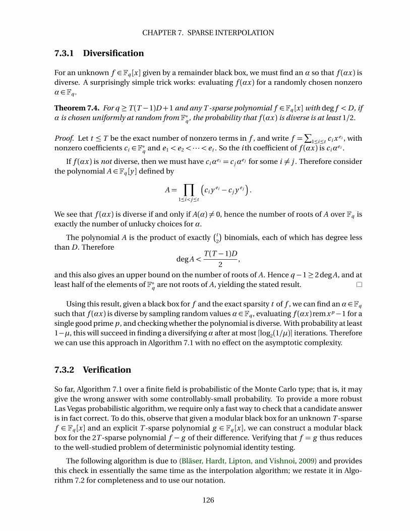
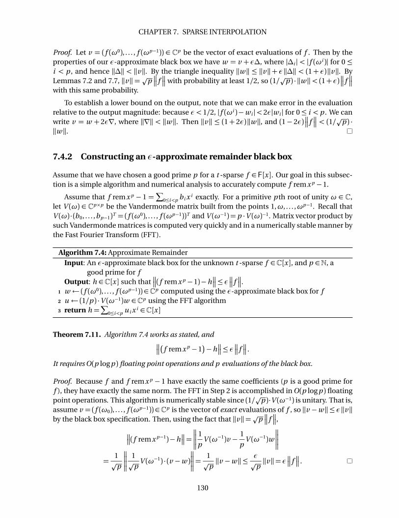
Proof. Let v = ( f (ω0), . . . , f (ωp−1)) ∈ Cp be the vector of exact evaluations of f . Then by theproperties of our ε-approximate black box we have w = v + ε∆, where |∆i | < | f (ωi )| for 0 ≤i < p , and hence ‖∆‖ < ‖v ‖. By the triangle inequality ‖w ‖ ≤ ‖v ‖+ ε‖∆‖ < (1+ ε)‖v ‖. ByLemmas 7.2 and 7.7, ‖v ‖=pp

f

with probability at least 1/2, so (1/pp ) · ‖w ‖< (1+ε)

f

with this same probability.

To establish a lower bound on the output, note that we can make error in the evaluationrelative to the output magnitude: because ε < 1/2, | f (ωi )−w i |< 2ε|w i | for 0≤ i < p . We canwrite v = w + 2ε∇, where ‖∇‖ < ‖w ‖. Then ‖v ‖ ≤ (1+ 2ε)‖w ‖, and (1− 2ε)

f

< (1/pp ) ·‖w ‖.

7.4.2 Constructing an ε-approximate remainder black box

Assume that we have chosen a good prime p for a t -sparse f ∈ F[x ]. Our goal in this subsec-tion is a simple algorithm and numerical analysis to accurately compute f remx p −1.

Assume that f remx p − 1 =∑

0≤i<p b i x i exactly. For a primitive p th root of unity ω ∈ C,let V (ω) ∈ Cp×p be the Vandermonde matrix built from the points 1,ω, . . . ,ωp−1. Recall thatV (ω) · (b0, . . . ,bp−1)T = ( f (ω0), . . . , f (ωp−1))T and V (ω−1) = p ·V (ω)−1. Matrix vector product bysuch Vandermonde matrices is computed very quickly and in a numerically stable manner bythe Fast Fourier Transform (FFT).

Algorithm 7.4: Approximate Remainder

Input: An ε-approximate black box for the unknown t -sparse f ∈C[x ], and p ∈N, agood prime for f

Output: h ∈C[x ] such that

( f remx p −1)−h

≤ ε

f

.1 w ← ( f (ω0), . . . , f (ωp−1))∈Cp computed using the ε-approximate black box for f2 u ← (1/p ) ·V (ω−1)w ∈Cp using the FFT algorithm3 return h =

∑

0≤i<p u i x i ∈C[x ]

Theorem 7.11. Algorithm 7.4 works as stated, and

f remx p −1

−h

≤ ε

f

.

It requires O(p log p ) floating point operations and p evaluations of the black box.

Proof. Because f and f remx p − 1 have exactly the same coefficients (p is a good prime forf ), they have exactly the same norm. The FFT in Step 2 is accomplished in O(p log p ) floatingpoint operations. This algorithm is numerically stable since (1/pp )·V (ω−1) is unitary. That is,assume v = ( f (ω0), . . . , f (ωp−1))∈Cp is the vector of exact evaluations of f , so ‖v −w ‖ ≤ ε‖v ‖by the black box specification. Then, using the fact that ‖v ‖=pp

f

,

( f remx p−1)−h

=

1

pV (ω−1)v −

1

pV (ω−1)w

=1p

p

1p

pV (ω−1) · (v −w )

=1p

p‖v −w ‖ ≤

εp

p‖v ‖= ε

f

.

130

CHAPTER 7. SPARSE INTERPOLATION

7.4.3 Creating ε-diversity

First, we extend the notion of polynomial diversity to the approximate case.

Definition 7.12. Let f ∈ C[x ] be a t -sparse polynomial as in (7.1) and δ ≥ ε > 0 such that|c i | ≥ δ

f

for 1 ≤ i ≤ t . The polynomial f is said to be ε-diverse if and only if every pair ofdistinct coefficients is at least ε

f

apart. That is, for every 1≤ i < j ≤ t , |c i − c j | ≥ ε

f

.

Intuitively, if (ε/2) corresponds to the machine precision, this means that an algorithm canreliably distinguish the coefficients of a ε-diverse polynomial. We now show how to choose arandom α to guarantee ε-diversity.

Theorem 7.13. Let δ ≥ ε > 0 and f ∈ C[x ] a t -sparse polynomial whose non-zero coefficientsare of magnitude at least δ

f

. If s is a prime satisfying s > 12 and

t (t −1)≤ s ≤ 3.1δ

ε,

then for ζ= e2πi/s an s -PRU and k ∈N chosen uniformly at random from 0, 1, . . . , s−1, f (ζk x )is ε-diverse with probability at least 1

2.

Proof. For each 1 ≤ i ≤ t , write the coefficient c i in polar notation to base ζ as c i = riζθi ,where each ri and θi are nonnegative real numbers and ri ≥δ

f

.

Suppose f (ζk x ) is not ε-diverse. Then there exist indices 1≤ i < j ≤ t such that

riζθiζk e i − rjζ

θjζk e j

≤ ε

f

.

Because min(ri , rj ) ≥ δ

f

, the value of the left hand side is at least δ

f

·

ζθi+k e i −ζθj+k e j

.Dividing out ζθj+k e i , we get

ζθi−θj −ζk (e j−e i )

≤ε

δ.

By way of contradiction, assume there exist distinct choices of k that satisfy the above in-equality, say k1, k2 ∈ 0, . . . , s −1. Since ζθi−θj and ζe j−e i are a fixed powers of ζ not dependingon the choice of k , this means

ζk1(e j−e i )−ζk2(e j−e i )

≤ 2ε

δ.

Because s is prime, e i 6= e j , and we assumed k1 6= k2, the left hand side is at least |ζ−1|.Observe that 2π/s , the distance on the unit circle from 1 to ζ, is a good approximation for thisEuclidean distance when s is large. In particular, since s > 12,

|ζ−1|2π/s

>

p2p

3−1

/2

π/6,

and therefore |ζ−1| > 6p

2(p

3− 1)/s > 6.2/s , which from the statement of the theorem is atleast 2ε/δ. This is a contradiction, and therefore the assumption was false; namely, there is atmost one choice of k such that the i ’th and j ’th coefficients collide.

Then, since there are exactlyt

2

distinct pairs of coefficients, and s ≥ t (t −1) = 2t

2

, f (ζk x )is diverse for at least half of the choices for k .

131

CHAPTER 7. SPARSE INTERPOLATION

Algorithm 7.5: Adaptive diversification

Input: ε-approximate black box for f , known good prime p , known sparsity tOutput: ζ, k such that f (ζk x ) is ε-diverse, or FAIL

1 s ← 1, δ←∞, f p ← 02 while s ≤ t 2 and #coeffs c of f s s.t. |c | ≥δ< t do3 s ← least prime ≥ 2s4 ζ← exp(2πi/s )5 k ← random integer in 0, 1, . . . , s −16 Compute f s = f (ζk x )remx p −17 δ← least number s.t. all coefficients of f s at least δ in absolute value are pairwise

ε-distinct

8 if δ> 2ε then return FAIL9 else return ζk

We note that the diversification which maps f (x ) to f (ζk x ) and back is numerically stablesince ζ is on the unit circle.

In practice, the previous theorem will be far too pessimistic. We therefore propose themethod of Algorithm 7.5 to adaptively choose s , δ, and ζk simultaneously, given a good primep .

Suppose there exists a threshold S ∈ N such that for all primes s > S, a random s th prim-itive root of unity ζk makes f (ζk x ) ε-diverse with high probability. Then Algorithm 7.5 willreturn a root of unity whose order is within a constant factor of S, with high probability. Fromthe previous theorem, if such an S exists it must be O(t 2), and hence the number of iterationsrequired is O(log t ).

Otherwise, if no such S exists, then we cannot diversify the polynomial. Roughly speaking,this corresponds to the situation that f has too many coefficients with absolute value close tothe machine precision. However, the diversification is not actually necessary in the approxi-mate case to guarantee numerical stability. At the cost of more evaluations, as well as the needto factor an integer polynomial, the algorithm of (Garg and Schost, 2009) for finite fields canbe adapted quite nicely for the approximate case. This is essentially the approach we outlinebelow, and even if the diversification step is omitted, the stated numerical properties of thecomputation will still hold true.

7.4.4 Approximate interpolation algorithm

We now plug our ε-approximate remainder black box, and method for making f ε-diverse,into our generic Algorithm 7.1 to complete our algorithm for approximate interpolation.

Theorem 7.14. Let δ > 0, f ∈C[x ] with degree at most D and sparsity at most T , and supposeall nonzero coefficients c of f satisfy |c | > δ

f

. Suppose also that ε < 1.5δ/(T (T − 1)), andwe are given an ε-approximate black box for f . Then, for any µ < 1/2 we have an algorithmto produce a g ∈ C[x ] satisfying the conditions of Theorem 7.9. The algorithm succeeds with

132

CHAPTER 7. SPARSE INTERPOLATION

probability at least 1−µ and uses O (T 2 · log(1/µ) · log2 D) black box evaluations and floatingpoint operations.

Proof. Construct an approximate remainder black box for f using Algorithm 7.4. Then runAlgorithm 7.1 using this black box as input. On step 8 of Algorithm 7.1, run Algorithm 7.5,iterating steps 5–7 dlog2(3/µ)e times on each iteration through the while loop to choose a di-versifying α= ζk with probability at least 1−µ/3.

The cost comes from Theorems 7.3 and 7.11 along with the previous discussion and The-orem 7.13.

Observe that the resulting algorithm is Monte Carlo, but could be made Las Vegas by com-bining the finite fields zero testing algorithm discussed in Section 7.3.2 with the guarantees ofTheorem 7.9.

7.5 Implementation results

We implemented our algorithms in the MVP library, using GMP (Granlund et al., 2010) andNTL (Shoup, 2009) for the exponent arithmetic. For comparison with the algorithm of Gargand Schost (2009), we also used NTL’s squarefree polynomial factorization routines. We notethat, in our experiments, the cost of integer polynomial factorization (for Garg & Schost) andChinese remaindering were always negligible.

In our timing results, “G&S Determ” refers to the deterministic algorithm as stated in Gargand Schost (2009) and “Alg 7.1” is the algorithm we have presented here over finite fields,without the verification step. We also developed and implemented a more adaptive, MonteCarlo version of these algorithms, as briefly described at the end of Section 7.2. The basicidea is to sample modulo x p − 1 for just one prime p ∈ Θ(t 2 log d ) that is good with highprobability, then to search for much smaller good primes. This good prime search starts ata lower bound of order Θ(t 2) based on the birthday problem, and finds consecutively largerprimes until enough primes have been found to recover the symmetric polynomial in theexponents (for Garg & Schost) or just the exponents (for our method). The correspondingimproved algorithms are referred to as “G&S MC” and “Alg 7.1++” in the table, respectively.

Table 7.3 summarizes some timings for these four algorithms on our benchmarking ma-chine. Note that the numbers listed reflect the base-2 logarithm of the degree bound and thesparsity bound for the randomly-generated test cases. The tests were all performed over the fi-nite field Z/65521Z. This modulus was chosen for convenience of implementation, althoughother methods such as the Ben-Or and Tiwari algorithm might be more efficient in this par-ticlar field since discrete logarithms could be computed quickly. However, observe that ouralgorithms (and those from Garg and Schost) have only poly-logarithmic dependence on thefield size, and so will eventually dominate.

The timings are mostly as expected based on our complexity estimates, and also confirmour suspicion that primes of size O(t 2) are sufficient to avoid exponent collisions. It is satis-fying but not particularly surprising to see that our “Alg 7.1++” is the fastest on all inputs, as

133

CHAPTER 7. SPARSE INTERPOLATION

log2 D T G&S Determ G&S MC Alg 7.1 Alg 7.1++12 10 3.77 0.03 0.03 0.0116 10 46.82 0.11 0.11 0.0820 10 — 0.38 0.52 0.3324 10 — 0.68 0.85 0.3828 10 — 1.12 2.35 0.5332 10 — 1.58 2.11 0.6612 20 37.32 0.15 0.02 0.0216 20 — 0.91 0.52 0.2820 20 — 3.5 3.37 1.9424 20 — 6.59 5.94 2.9928 20 — 10.91 10.22 3.7132 20 — 14.83 16.22 4.2412 30 — 0.31 0.01 0.0116 30 — 3.66 1.06 0.6520 30 — 10.95 6.7 3.5624 30 — 25.04 12.42 9.3228 30 — 38.86 19.36 13.832 30 — 62.53 68.1 14.6612 40 — 0.58 0.01 0.0216 40 — 8.98 3.7 1.5420 40 — 30.1 12.9 8.4224 40 — 67.97 38.34 16.5728 40 — — 73.69 36.2432 40 — — — 40.79

Table 7.3: Finite Fields Algorithm Timings

134

CHAPTER 7. SPARSE INTERPOLATION

Noise Mean Error Median Error Max Error0 4.440 e−16 4.402 e−16 8.003 e−16±10−12 1.113 e−14 1.119 e−14 1.179 e−14±10−9 1.149 e−11 1.191 e−11 1.248 e−11±10−6 1.145 e−8 1.149 e−8 1.281 e−8

Table 7.4: Approximate Algorithm Stability

all the algorithms have a similar basic structure. Had we compared to the Ben-Or and Tiwarior Zippel’s method, they would probably be more efficient for small sizes, but would be easilybeaten for large degree and arbitrary finite fields as their costs are super-polynomial.

The implementation of the approximate algorithm uses machinedoubleprecision (basedon the IEEE standard), the built-in C++ complex<double> type, and the popular FastestFourier Transform in the West (FFTW) package for computing FFTs (Frigo and Johnson, 2005).Our stability results are summarized in Table 7.4. Each test case was randomly generated withdegree at most 220 and at most 50 nonzero terms. We varied the precision as specified in thetable and ran 10 tests in each range. Observe that the error in our results was often less thanthe ε error on the evaluations themselves.

7.6 Conclusions

We have presented two new algorithms, using the basic idea of Garg and Schost (2009), plusour new technique of diversification, to gain improvements for sparse interpolation over largefinite fields and approximate complex numbers.

There is much room for improvement in both of these methods. For the case of finitefields, the limitation to large finite fields of size at leastΩ(t 2d n ) is in some sense the interestingcase, since for very small finite fields it will be faster to use Ben-Or and Tiwari’s algorithm andcompute the discrete logs as required. However, the restriction on field size for our algorithmsdoes seem rather harsh, and we would like to reduce it, perhaps to a bound of size only t O(1).This would have a tremendous advantage because working in an extension field to guaranteethat size would only add a logarithmic factor to the overall complexity. By contrast, workingan extension large enough to satisfy the conditions of our algorithm could add a factor ofO (log d ) to the complexity, which is significant for lacunary algorithms.

Over approximate complex numbers, our algorithm provides the first provably numeri-cally stable method for sparse interpolation. However, this improved numerical stability is atthe expense of extra computational cost and (more significantly) extra black-box probes. Formany applications, the cost of probing the unknown function easily dominates the cost ofthe interpolation algorithm, and therefore reducing the number of probes as much as possi-ble is highly desirable. Ideally, we would like to have an approximate interpolation algorithmwith the numerical stability of ours, but using only O(t ) probes, as in Ben-Or and Tiwari’salgorithm.

135

CHAPTER 7. SPARSE INTERPOLATION

Another area for potential improvement is in the bounds used for the number of possiblebad primes, in both algorithms. From our experiments and intuition, it seems that usingprimes of size roughly O(t 2+ t log d ) should be sufficient, rather than the O(t 2 log d ) size ourcurrent bounds require. However, proving this seems quite challenging. These and otherrelated bounds will be discussed at greater length in the next chapter.

136

Bibliography

Martín Avendaño, Teresa Krick, and Ariel Pacetti. Newton-Hensel interpolation lifting. Found.Comput. Math., 6(1):81–120, 2006. ISSN 1615-3375.doi: 10.1007/s10208-005-0172-3. Referenced on page 121.

Eric Bach and Jeffrey Shallit. Algorithmic number theory. Vol. 1. Foundations of ComputingSeries. MIT Press, Cambridge, MA, 1996. ISBN 0-262-02405-5. Referenced on page 127.

Michael Ben-Or and Prasoon Tiwari. A deterministic algorithm for sparse multivariate poly-nomial interpolation. In Proceedings of the twentieth annual ACM symposium on Theory ofcomputing, STOC ’88, pages 301–309, New York, NY, USA, 1988. ACM. ISBN 0-89791-264-0.doi: 10.1145/62212.62241. Referenced on pages 119 and 122.

Markus Bläser, Moritz Hardt, Richard J. Lipton, and Nisheeth K. Vishnoi. Deterministicallytesting sparse polynomial identities of unbounded degree. Information Processing Letters,109(3):187 – 192, 2009. ISSN 0020-0190.doi: 10.1016/j.ipl.2008.09.029. Referenced on page 126.

John F. Canny, Erich Kaltofen, and Lakshman Yagati. Solving systems of nonlinear polyno-mial equations faster. In Proceedings of the ACM-SIGSAM 1989 international symposium onSymbolic and algebraic computation, ISSAC ’89, pages 121–128, New York, NY, USA, 1989.ACM. ISBN 0-89791-325-6.doi: 10.1145/74540.74556. Referenced on page 118.

Michael Clausen, Andreas Dress, Johannes Grabmeier, and Marek Karpinski. On zero-testingand interpolation of k -sparse multivariate polynomials over finite fields. Theoretical Com-puter Science, 84(2):151–164, 1991. ISSN 0304-3975.doi: 10.1016/0304-3975(91)90157-W. Referenced on page 118.

Annie Cuyt and Wen-shin Lee. A new algorithm for sparse interpolation of multivariate poly-nomials. Theoretical Computer Science, 409(2):180–185, 2008. ISSN 0304-3975.doi: 10.1016/j.tcs.2008.09.002. Symbolic-Numerical Computations. Referenced onpage 122.

Richard A. Demillo and Richard J. Lipton. A probabilistic remark on algebraic program testing.Information Processing Letters, 7(4):193–195, 1978. ISSN 0020-0190.doi: 10.1016/0020-0190(78)90067-4. Referenced on page 118.

157

Angel Díaz and Erich Kaltofen. On computing greatest common divisors with polynomialsgiven by black boxes for their evaluations. In Proceedings of the 1995 international sym-posium on Symbolic and algebraic computation, ISSAC ’95, pages 232–239, New York, NY,USA, 1995. ACM. ISBN 0-89791-699-9.doi: 10.1145/220346.220375. Referenced on page 118.

Angel Díaz and Erich Kaltofen. FOXBOX: a system for manipulating symbolic objects in blackbox representation. In Proceedings of the 1998 international symposium on Symbolic andalgebraic computation, ISSAC ’98, pages 30–37, New York, NY, USA, 1998. ACM. ISBN 1-58113-002-3.doi: 10.1145/281508.281538. Referenced on page 118.

Matteo Frigo and Steven G. Johnson. The design and implementation of FFTW3. Proceedingsof the IEEE, 93(2):216–231, 2005. Special issue on “Program Generation, Optimization, andPlatform Adaptation”. Referenced on page 135.

Sanchit Garg and Éric Schost. Interpolation of polynomials given by straight-line programs.Theoretical Computer Science, 410(27-29):2659–2662, 2009. ISSN 0304-3975.doi: 10.1016/j.tcs.2009.03.030. Referenced on pages 117, 119, 122, 123, 127, 132, 133and 135.

Joachim von zur Gathen and Jürgen Gerhard. Modern Computer Algebra. Cambridge Univer-sity Press, Cambridge, second edition, 2003. ISBN 0521826462. Referenced on page 119.

Mark Giesbrecht, George Labahn, and Wen-shin Lee. Symbolic-numeric sparse interpolationof multivariate polynomials. Journal of Symbolic Computation, 44(8):943 – 959, 2009. ISSN0747-7171.doi: 10.1016/j.jsc.2008.11.003. Referenced on page 122.

Torbjörn Granlund et al. GNU Multiple Precision Arithmetic Library, The. Free Software Foun-dation, Inc., 4.3.2 edition, January 2010.URL http://gmplib.org/. Referenced on page 133.

Dima Yu. Grigoriev, Marek Karpinski, and Michael F. Singer. Fast parallel algorithms for sparsemultivariate polynomial interpolation over finite fields. SIAM Journal on Computing, 19(6):1059–1063, 1990.doi: 10.1137/0219073. Referenced on page 121.

Wassily Hoeffding. Probability inequalities for sums of bounded random variables. J. Amer.Statist. Assoc., 58:13–30, 1963. ISSN 0162-1459.URL http://www.jstor.org/stable/2282952. Referenced on page 125.

Seyed Mohammad Mahdi Javadi and Michael Monagan. A sparse modular GCD algorithm forpolynomials over algebraic function fields. In Proceedings of the 2007 international sym-posium on Symbolic and algebraic computation, ISSAC ’07, pages 187–194, New York, NY,USA, 2007. ACM. ISBN 978-1-59593-743-8.doi: 10.1145/1277548.1277575. Referenced on page 118.

158

Seyed Mohammad Mahdi Javadi and Michael Monagan. On factorization of multivariatepolynomials over algebraic number and function fields. In Proceedings of the 2009 interna-tional symposium on Symbolic and algebraic computation, ISSAC ’09, pages 199–206, NewYork, NY, USA, 2009. ACM. ISBN 978-1-60558-609-0.doi: 10.1145/1576702.1576731. Referenced on page 118.

Seyed Mohammad Mahdi Javadi and Michael Monagan. Parallel sparse polynomial interpo-lation over finite fields. In Proceedings of the 4th International Workshop on Parallel andSymbolic Computation, PASCO ’10, pages 160–168, New York, NY, USA, 2010. ACM. ISBN978-1-4503-0067-4.doi: 10.1145/1837210.1837233. Referenced on page 121.

Valentine Kabanets and Russell Impagliazzo. Derandomizing polynomial identity tests meansproving circuit lower bounds. Computational Complexity, 13:1–46, 2004. ISSN 1016-3328.doi: 10.1007/s00037-004-0182-6. 10.1007/s00037-004-0182-6. Referenced on page118.

Erich Kaltofen and Wen-shin Lee. Early termination in sparse interpolation algorithms. Jour-nal of Symbolic Computation, 36(3-4):365–400, 2003. ISSN 0747-7171.doi: 10.1016/S0747-7171(03)00088-9. ISSAC 2002. Referenced on page 121.

Erich Kaltofen and Barry M. Trager. Computing with polynomials given by black boxes fortheir evaluations: Greatest common divisors, factorization, separation of numerators anddenominators. Journal of Symbolic Computation, 9(3):301–320, 1990. ISSN 0747-7171.doi: 10.1016/S0747-7171(08)80015-6. Computational algebraic complexity editorial.Referenced on page 118.

Erich Kaltofen and Lakshman Yagati. Improved sparse multivariate polynomial interpolationalgorithms. In P. Gianni, editor, Symbolic and Algebraic Computation, volume 358 of LectureNotes in Computer Science, pages 467–474. Springer Berlin /Heidelberg, 1989.doi: 10.1007/3-540-51084-2_44. Referenced on pages 119 and 121.

Erich Kaltofen and Zhengfeng Yang. On exact and approximate interpolation of sparse ratio-nal functions. In Proceedings of the 2007 international symposium on Symbolic and alge-braic computation, ISSAC ’07, pages 203–210, New York, NY, USA, 2007. ACM. ISBN 978-1-59593-743-8.doi: 10.1145/1277548.1277577. Referenced on page 122.

Erich Kaltofen, Y. N. Lakshman, and John-Michael Wiley. Modular rational sparse multivariatepolynomial interpolation. In Proceedings of the international symposium on Symbolic andalgebraic computation, ISSAC ’90, pages 135–139, New York, NY, USA, 1990. ACM. ISBN 0-201-54892-5.doi: 10.1145/96877.96912. Referenced on page 121.

Erich Kaltofen, Zhengfeng Yang, and Lihong Zhi. On probabilistic analysis of randomizationin hybrid symbolic-numeric algorithms. In Proceedings of the 2007 international workshopon Symbolic-numeric computation, SNC ’07, pages 11–17, New York, NY, USA, 2007. ACM.

159

ISBN 978-1-59593-744-5.doi: 10.1145/1277500.1277503. Referenced on page 122.

Erich Kaltofen, John P. May, Zhengfeng Yang, and Lihong Zhi. Approximate factorization ofmultivariate polynomials using singular value decomposition. Journal of Symbolic Compu-tation, 43(5):359–376, 2008. ISSN 0747-7171.doi: 10.1016/j.jsc.2007.11.005. Referenced on page 118.

Erich L. Kaltofen. Fifteen years after DSC and WLSS2: What parallel computations I do today[invited lecture at PASCO 2010]. In Proceedings of the 4th International Workshop on Paralleland Symbolic Computation, PASCO ’10, pages 10–17, New York, NY, USA, 2010. ACM. ISBN978-1-4503-0067-4.doi: 10.1145/1837210.1837213. Referenced on pages 119 and 120.

Yishay Mansour. Randomized interpolation and approximation of sparse polynomials. SIAMJournal on Computing, 24(2):357–368, 1995.doi: 10.1137/S0097539792239291. Referenced on page 122.

J. M. Pollard. Monte Carlo methods for index computation (mod p ). Math. Comp., 32(143):918–924, 1978. ISSN 0025-5718.doi: 10.1090/S0025-5718-1978-0491431-9. Referenced on page 119.

J. M. Pollard. Kangaroos, monopoly and discrete logarithms. Journal of Cryptology, 13:437–447, 2000. ISSN 0933-2790.doi: 10.1007/s001450010010. Referenced on page 119.

J. Barkley Rosser and Lowell Schoenfeld. Approximate formulas for some functions of primenumbers. Ill. J. Math., 6:64–94, 1962.URL http://projecteuclid.org/euclid.ijm/1255631807. Referenced on page 123.

Nitin Saxena. Progress on polynomial identity testing. Bull. EATCS, 99:49–79, 2009. Refer-enced on page 118.

J. T. Schwartz. Fast probabilistic algorithms for verification of polynomial identities. J. ACM,27:701–717, October 1980. ISSN 0004-5411.doi: 10.1145/322217.322225. Referenced on page 118.

Victor Shoup. NTL: A Library for doing Number Theory. Online, August 2009.URL http://www.shop.net/ntl/. Version 5.5.2. Referenced on page 133.

Amir Shpilka and Amir Yehudayoff. Arithmetic circuits: A survey of recent results and openquestions. Foundations and Trends in Theoretical Computer Science, 5(3-4):207–388, 2010.Referenced on page 118.

A. J. Sommese and C. W. Wampler. Numerical solution of polynomial systems arising in engi-neering and science. World Scientific, Singapore, 2005. Referenced on page 118.

160

Andrew J. Sommese, Jan Verschelde, and Charles W. Wampler. Numerical decompositionof the solution sets of polynomial systems into irreducible components. SIAM Journal onNumerical Analysis, 38(6):2022–2046, 2001.doi: 10.1137/S0036142900372549. Referenced on page 118.

Andrew J. Sommese, Jan Verschelde, and Charles W. Wampler. Numerical factorization ofmultivariate complex polynomials. Theoretical Computer Science, 315(2-3):651–669, 2004.ISSN 0304-3975.doi: 10.1016/j.tcs.2004.01.011. Referenced on page 118.

Hans J. Stetter. Numerical Polynomial Algebra. Society for Industrial and Applied Mathemat-ics, Philadelphia, PA, USA, 2004. ISBN 0898715571. Referenced on page 118.

Richard Zippel. Probabilistic algorithms for sparse polynomials. In Edward Ng, editor, Sym-bolic and Algebraic Computation, volume 72 of Lecture Notes in Computer Science, pages216–226. Springer Berlin /Heidelberg, 1979.doi: 10.1007/3-540-09519-5_73. Referenced on page 118.

Richard Zippel. Interpolating polynomials from their values. Journal of Symbolic Computa-tion, 9(3):375–403, 1990. ISSN 0747-7171.doi: 10.1016/S0747-7171(08)80018-1. Computational algebraic complexity editorial.Referenced on pages 120 and 121.

161