This document is not an API Standard; it is under consideration within an API technical committee but has not received all approvals required to become an API Standard. It shall not be reproduced or circulated or quoted, in whole or in part, outside of API committee activities except with the approval of the Chairman of the committee having jurisdiction and staff of the API Standards Dept. Copyright API. All rights reserved.

1 

Chapter 4—Proving Systems Section 6—Pulse Interpolation

1 Introduction

To prove meters that have pulsed outputs, a minimum number of pulses must be collected during the proving period, depending on the user’s chosen meter technology. Limits on prover volume or the number of pulses that a flowmeter can produce per unit quantity of throughput can limit design considerations.

The electronic signal from a flowmeter allows for interpolation between adjacent pulses. The technique of improving the discrimination of a flowmeter’s output is known as pulse interpolation. Although pulse-interpolation techniques were originally intended for use with small volume provers, they can also be applied to other proving devices. Pulse interpolation, though a mathematical technique, relies on the underlying and contributing uncertainty of the prover detector signal. Potential users are cautioned that use of the technique absent the requisite accuracy can produce misleading results.

The pulse-interpolation method known as double-chronometry, described in this chapter, is an established technique used in proving flowmeters. As other methods of pulse interpolation become accepted industry practice, they should receive equal consideration, provided that they can meet the established verification tests and specifications described in this publication.

2 Scope

This chapter describes how the double-chronometry method of pulse interpolation, including system operating requirements and equipment testing, is applied to meter proving.

3 Definitions

For the purposes of this document the following terms and definitions apply. Terms of more general use may be found the API MPMS Chapter 1, Online Terms and Definitions Database. Acronyms are defined in the test at first use. 3.1 detector signal A contact closure change or other signal to a prover counter, timer or flow computer/RTU that defines the start or end of the calibrated volume of the prover.

3.2 double-chronometry (Dual Chronometry) A pulse interpolation technique used to increase the discrimination level of flowmeter pulses detected between prover detector signals. This is accomplished by resolving these pulses into a whole number of pulses plus a fractional part of a pulse using two high speed timers, associated logic, detector signals and the flowmeter pulses.

3.3 flowmeter discrimination A measure of the smallest increment of change in the pulses per unit of the quantity being measured.

2

3.4 frequency The number of repetitions, or cycles, of a periodic signal (for example, pulses, alternating voltage, or current) occurring in a 1-second time period. The number of repetitions, or cycles, that occur in a 1-second period is expressed in hertz.

3.5 meter pulse continuity The deviation of the inter-pulse period of a flowmeter expressed as a percentage of a full pulse period.

3.6 nonrotating meter Any metering device for which the meter pulse output is not derived from mechanical rotation as driven by the flowing stream. For example, vortex shedding, venturi tubes, orifice plates, sonic nozzles, and ultrasonic, direct mass flow meters (Coriolis) and electromagnetic flowmeters are metering devices for which the output is derived from some characteristic other than rotation that is proportional to flow rate.

3.7 pulse period The reciprocal of pulse frequency, i.e., a pulse frequency of 2 hertz, is equal to a pulse period of 1/2 seconds.

3.8 pulse generator An electronic device that can be programmed to output voltage pulses of a precise frequency or time period.

3.9 pulse interpolation Any of the various techniques by which the meter pulses are counted between two events (such as detector switch closures); whereby, any remaining fraction of a pulse between the two events is calculated.

3.10 rotating meter Any metering device for which the meter pulse output is derived from mechanical rotation as driven by the flowing stream. For example, turbine and positive displacement meters are those metering devices for which the output is derived from the continuous angular displacement of a flow-driven member.

3.11 signal-to-noise ratio The ratio of the magnitude of the electrical signal to that of the electrical noise.

4 References

The following referenced documents are indispensable for the application of this document. For dated references only the edition cited applies. For undated references, the latest edition of the reference document (including any amendments) applies.

MPMS Chapter 4, Proving Systems, Section 2, “Displacement Provers”

MPMS Chapter 4, Proving Systems, Section 8, “Operation of Proving Systems”

3

MPMS Chapter 5, Metering, Section 4, “Instrumentation and Auxiliary Equipment for Liquid Hydrocarbon Metering Systems”

MPMS Chapter 5, Metering, Section 5, “Security and Fidelity of Pulse Data”

MPMS Chapter 12.2.3 “Calculation of Petroleum Quantities Using Dynamic Measurement Methods and Volumetric Correction Factors, Proving Reports”

5 Double-Chronometry Pulse Interpolation

5.1 General

Double-chronometry pulse interpolation requires counting the total integer (whole) number of flowmeter pulses, Nm, generated during the proving run and measuring the time intervals, T1 and T2. T1 is the time interval between the first flowmeter pulse after the first detector signal and the first flowmeter pulse after the last detector signal. T2 is the time interval between the first and last detector signals.

The pulse counters, or timers, are started and stopped by the signals from the prover detector or detectors. The time intervals T1, corresponding to Nm pulses, and T2, corresponding to the interpolated number of pulses (N1), are measured by an accurate clock. The interpolated pulse count is given as follows:

N1 = Nm (T2/T1)

The use of double-chronometry in meter proving requires that the discrimination of the time intervals T1 and T2 be better than ± 0.01%. The time periods T1 and T2 shall therefore be at least 20,000 times greater than the reference period Tc of the clock that is used to measure the time intervals. The clock frequency Fc must be high enough to ensure that both the T1 and T2 timers accumulate at least 20,000 clock pulses during the prove operation. This is not difficult to achieve, as current electronics technology used for pulse interpolation typically uses clock frequencies in the megahertz range.

5.2 Conditions of Use

The interpolated number of pulses, N1, will not be a whole number. N1 is therefore rounded off as described in MPMS Chapter 12.2, Part 3.

Pulse-interpolation methods are based on the assumptions that actual flow rate does not change substantially during the period between successive meter pulses, and each pulse represents the same volume. Refer to MPMS Chapter 4.2, Annex E for Pulse Stability. To maintain the validity of these assumptions, short period fluctuations in the flow rate during the proving operation shall be minimized.

Because pulse interpolation equipment contains high speed counters and timers, it is important that equipment be installed in accordance with the manufacturer’s installation instructions, thereby minimizing the risk of counting spurious pulses caused by electrical interference occurring during the proving operation. Refer to MPMS Chapter 5.4, MPMS Chapter 5.5, and other sections of Chapter 4 for more details.

5.3 Flowmeter Operating Requirements

The flowmeter that is being proved and is providing the pulses for the pulse-interpolation system shall meet the following requirements:

a) If the pulse stability at constant flow rate cannot be maintained within the limits given in MPMS Chapter 4.2, Annex E, then the flowmeter can be used with a pulse-interpolation system only at a lower overall accuracy level. In this case, a revised calibration accuracy level should be evaluated or multiple runs with summation techniques employed. See MPMS Chapter 4.8.

4

b) The meter pulse continuity in flowmeters should be in accordance with MPMS Chapter 4.2, Annex E. The generated flowmeter pulse can be observed by an oscilloscope, whose time base is set to a minimum of one full cycle, to verify meter pulse continuity of the flowmeter.

c) The repeatability of the flowmeters will be a function of the rate of change in pulse frequency at a constant flow rate. To apply pulse-interpolation techniques to any flowmeter, the meter pulse stability of the flowmeter should be in accordance with MPMS Chapter 4.2, Annex E.

d) The size and shape of the signal generated by the flow meter should be suitable for presentation to the pulse-interpolation system in terms of duty cycle, proportionality and interpulse spacing. If necessary, the signal should undergo amplification and shaping before it enters the pulse-interpolation system.

6 Electronic Equipment Calculation Testing

The proper operation of pulse interpolation electronics is crucial to accurate meter proving. A functional field test of the total system should be performed periodically to ensure that the equipment is calculating correctly. This may simply be a hand calculation verifying that the equipment correctly calculates the interpolated pulses per Section 5, or if need be, a complete certification test as described in Section 8, if a problem is suspected.

6.1 Functional Operations Test Requirements

The system being used should provide diagnostic data displays or printed data reports which show the value of all parameters and variables necessary to verify proper operation of the system by hand calculation. These parameters and variables include, but are not limited to, timers T1 and T2, the number of whole flowmeter pulses Nm and the calculated interpolated pulses N1.

Using the diagnostic displays provided, the unit should be functionally tested by performing a sequence of prove runs and analyzing the displayed or printed results.

6.2 Certification Test

Certification tests should be performed by the manufacturer prior to shipment of the equipment, and if necessary, by the user on a scheduled basis, or as mutually agreed upon by all interested parties. The certification tests provided in this chapter do not preclude the use of other tests that may be performed on an actual field installation.

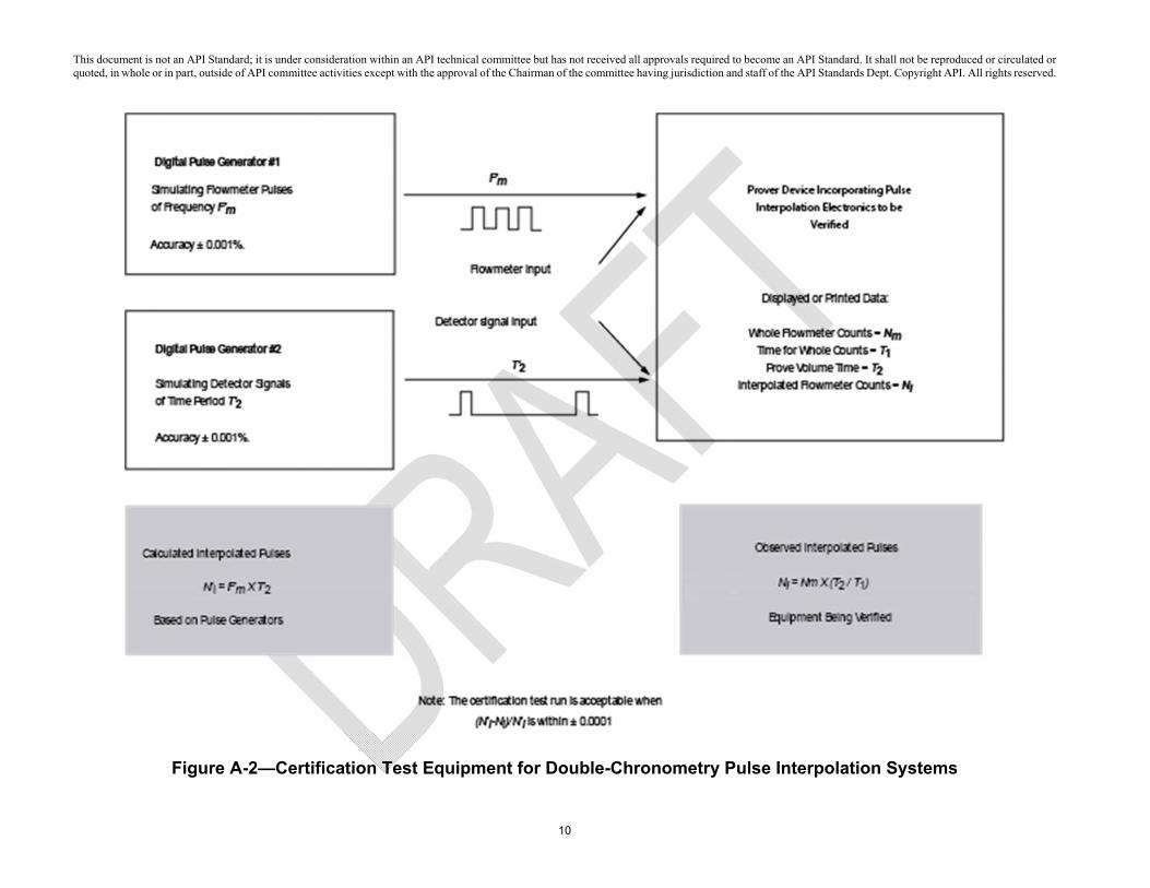
A block diagram of the certification test equipment is provided in Figure A-2.

An adjustable, certified, and traceable pulse generator with an output uncertainty equal to or less than 0.001% is installed that provides an output signal of frequency F'm, simulating a flowmeter pulse train. This signal is connected to the flowmeter input of the pulse interpolation device.

A second adjustable, certified, and traceable pulse generator with an output uncertainty equal to or less than 0.001% is installed that provides an output pulse signal separated by time period T'2, simulating the detector switch signals. This signal is connected to the detector switch inputs of the pulse interpolation device.

The pulse interpolation function is more critical when there are fewer flowmeter pulses collected between the detector switches. Set the output frequency of the first generator to produce a frequency equal to the flowmeter that has the lowest number of pulses per unit volume to be proved with the equipment, at the highest proving flowrate expected.

The pulse interpolation function is also more critical when there are fewer clock pulses collected between the detector switches. Set the pulse period of the second generator to provide a volume time, T'2, equal to that which would be produced by the prover detectors at the fastest proving flowrate expected.

5

Example: A small volume prover with a waterdraw volume of 0.81225 barrels will be used to prove a turbine meter (K Factor 1000 pulses per barrel) at a maximum of 3000 barrels per hour.

Volume time T2 for 0.81225 barrels at 3000 barrels per hour:

= 3600 x 0.81225 / 3000

T2 = 0.9747

Flowmeter frequency Fm produced by flowmeter (K Factor 1000) at 3000 barrels per hour:

= 3000 x 1000 / 3600

F'm = 833.33333 hertz.

The calculated interpolated flowmeter pulses N'1 are simply the simulated flowmeter frequency F'm times the simulated volume time T'2.

= 833.33333 x 0.9747

N1 = 812.2491

Verify the actual results displayed or printed by the pulse interpolation device under test, ensuring that they are within ± 0.01% of the calculated value.

It is possible to select a simulation frequency F'm above whose pulse period is an exact multiple of time period T'2, thereby synchronizing the simulated flowmeter pulses and detector signals. If this is the case, it will be necessary to modify either the simulated flowmeter frequency F'm, or the simulated detector switch period T'2 slightly to ensure that the interpolated pulses will include a fractional part of a pulse.

7 Manufacturer’s Certification Tests

Certification tests should be performed at a number of simulated conditions. These conditions should encompass the prover device’s range of prover volume times, T2, and flowmeter pulse frequencies, Fm. The manufacturer must provide, on request, a test certificate detailing the maximum and mini- mum values of prover volume time, T2, and flowmeter frequency, Fm, that the equipment is designed to accept.

If the pulse-interpolation electronics are tested and verified, they can be used during a flowmeter proving operation with confidence that they will contribute an error of less than ± 0.01% to the overall accuracy of the proving operations within the pulse-signal-frequency range tested.

This document is not an API Standard; it is under consideration within an API technical committee but has not received all approvals required to become an API Standard. It shall not be reproduced or circulated or quoted, in whole or in part, outside of API committee activities except with the approval of the Chairman of the committee having jurisdiction and staff of the API Standards Dept. Copyright API. All rights reserved.

6 

Annex A (normative)

Pulse-Interpolation Calculations

A.1 General

The double-chronometry method of pulse interpolation is described in Section 4. Figure A-1 is a diagram of the electrical signals required for the technique. The technique provides the numerical data required to resolve a fractional portion of a single whole flowmeter pulse. Double-chronometry pulse interpolation requires using the following three electrical counters: CTR-Nm to count whole flowmeter pulses, CTR-T1 to count the time required to accumulate the whole flowmeter pulses, and CTR-T2 to count the time between detector signals, which define the displaced prover volume.

The double-chronometry technique reduces the total number of whole flowmeter pulses normally required for the displaced volume to fewer than 10,000 to achieve a discrimination uncertainty of 0.02% (± 0.01% of the average) for a proof run.

The required time/pulse discrimination guidelines are presented in Sect ion 4 and shall be used in conjunction with a prover designed in accordance with the sizing parameters described in MPMS Chapter 4.2.

The examples given in A.2, which conform to the guidelines in Section 4, each represent a single case of defined data and are not necessarily representative of all available pulse-interpolation methods.

A.2 Examples

The following data are given:

Fc = clock frequency used to measure the time intervals, in hertz > (20,000/Nl) Fm

Fm = flowmeter pulse output frequency (the maximum value for analysis), in hertz = 520

Nm = total number of whole flowmeter pulses = 200 (CTR-Nm)

NI = number of interpolated flowmeter pulses = (T2/T1) Nm

T1 = time interval counted for the whole flowmeter pulses (N) in seconds = 2.43914 (CTR-T1)

T2 = time interval between the first and second volume detector signals (that is, the displaced prover volume), in seconds = 2.43917 (CTR-T2)

If the required pulse-interpolation uncertainty is better than ± 0.01 %, then:

100,000 > (20,000/200 pulses)(520 hertz)

> (100)(520)

> 52,000

7

NOTE The period of the clock is the reciprocal of the frequency, T = 0.00001 second. The discrimination of the clock is 0.00001/ 2.43914, or 0.0004 %. The requirement for the value of Fc and the discrimination requirement in 4.6.2 are therefore satisfied.

To calculate the interpolated pulses,

N1 = (2.43917 / 2.43914)(200)

= (1.00001)(200)

= 200.002

A.2.2 EXAMPLE 2—CERTIFICATION CALCULATION

Using equipment as shown in Figure A-2, the following data applies:

Simulated data:

F’m = pulse frequency of generator number one simulating meter pulses, in hertz = 233.000

T’2 = pulse period of generator number two simulating detector signals, in seconds = 1.666667

Observed data at prover computer being tested:

Nm = number of whole flowmeter pulses = 388

T1 = number of clock pulses accumulated during whole flowmeter counts Nm = 166,523

T2 = number of clock pulses accumulated during simulated prove volume = 166,666

Note that both timers T1 and T2 accumulated > 20,000 clock pulses, satisfying the discrimination requirement detailed in 4.6.2.

Comparison of results:

N'1 = calculated interpolated pulses based on certified pulse generators,

= F'm x T'2

= 233 x 1.666667

= 388.33341

N1 = calculated interpolated pulses based on prover computer observations,

= Nm (T2/T1)

= 388 x 166666/166523

= 388.33319

The certification test agreement required between N'1 and N1, is better than ± 0.01 %, then:

(N'1 – N1)/N'1 < 0.0001

8

(388.33341 – 388.33319) / 388.33341 = 0.0000005

The test device results agree with calculated results based on traceable pulse generator data within 0.00005%. The certification test run is acceptable.

This document is not an API Standard; it is under consideration within an API technical committee but has not received all approvals required to become an API Standard. It shall not be reproduced or circulated or quoted, in whole or in part, outside of API committee activities except with the approval of the Chairman of the committee having jurisdiction and staff of the API Standards Dept. Copyright API. All rights reserved.

9 

Figure A-1—Double-Chronometry Timing Diagram

This document is not an API Standard; it is under consideration within an API technical committee but has not received all approvals required to become an API Standard. It shall not be reproduced or circulated or quoted, in whole or in part, outside of API committee activities except with the approval of the Chairman of the committee having jurisdiction and staff of the API Standards Dept. Copyright API. All rights reserved.

10 

Figure A-2—Certification Test Equipment for Double-Chronometry Pulse Interpolation Systems

11

ANNEX B (normative)

Pulse-Interpolation Calculations

B.1 Pulse Interpolation Verification

The pulse interpolation test assembly requires a stable high speed, free running clock which is divided down by a fixed divider value to produce the lower speed simulated meter pulses, which are injected into the flow computer under test. It will then sim-ulate the detector switches DS1 and DS2 at programmable and highly repeatable intervals, with a fixed phase relationship to the simulated meter pulses. The divider value should be a minimum of 100, a higher divider ratio will allow finer resolution of fractional numbers generated (but, note, not a higher accuracy). Clock speeds of 1 MHz or greater are required. The requirement of a “a stable high speed, free running clock” virtually eliminates the use of digitally synthesized frequencies. Before the simulation is started the following parameters need to be set: 1. The divider ratio "Dr" is a programmable value. The frequency of the high-speed clock divided by "Dr" gives the meter pulse frequency. 2. The number of whole meter pulses to be collected 3. A launch delay representative of a specific number of high speed clock pulses. 4. An offset value in terms of fractional meter pulses for DS1 (Note: the DS1 counter will be loaded with the value of the Divider ratio minus the DS1 negative offset)

5. An offset value in terms of fractional meter pulses (high speed clock pulses) for DS2.

Tests should be conducted at both the minimum and the maximum input frequency of the device under test.

A prove simulation cycle can be initiated by a digital output from the flow computer under test, or from a push button on the simulator.

12

B.2 Figure A. Upon receiving the Launch signal, the launch delay timer will start, and when the predetermined launch delay has expired, the simulator will wait until the next leading edge of the low-speed "Meter Pulses", designated pulse "-1" in the example drawing. When the leading edge is detected, the DS1 timer will start to count the high-speed master clock pulse. In the example drawing, the divider ratio, Dr is set to 100 and the DS1 count has been set to 7. After 7 of the high-speed clocks have been counted, Detector Switch DS1 will be generated. This would mean that DS1 is generated 3/10th of a meter pulse BEFORE meter pulse "0". A low speed counter then counts the whole number of meter pulses, and when the desired whole number is reached (1000in the example), the DS2 high speed counter is triggered. In the example drawing, the DS2 offset has been set at 6, and when 6 high speed pulses have been counted, Detector Switch DS2 is triggered, 6/10ths of a meter pulse after the 1000th meter pulse. In this example, the clock speed is 100 times that of the meter pulse frequency. Assuming a meter frequency of 10,000 Hz, the high clock speed is 1 MHz. The results from the flow computer under test should be 1000.900 pulses. B.3 Clocks And Counters There is a counter synchronized with the low speed (divided down count) a clock for the whole number of pulses requested and two counters synchronized with the high speed (master) clock. The two high speed counters are also programmable. The first determines how many high-speed clock pulses are before the first meter pulse (Divider Ratio – Offset) and high-speed counter 2 determines how many high-speed clock ticks there are after the “Nth” meter pulse (10,000 in the example) and DS2.

13