Chapter 7 Sampling Distributions General Objectives: We begin to study samples and the statistics that describe them. These samples statistics are used

Chapter 7 Sampling Distributions

General Objectives:

We begin to study samples and the statistics that describe them. These samples statistics are used to make inferences about the corresponding population parameters. This chapter involves sampling and sampling distributions, which describe the behavior of sample statistics in repeated sampling.

©1998 Brooks/Cole Publishing/ITP

Specific Topics

1. Random samples

2. Sampling plans and experimental designs

3. Statistics and sampling distributions

4. The central limit theorem

5. The sampling distribution of the sample mean,

6. The sampling distribution of the sample proportion,

7. Statistical process control: and p charts


x

p̂

x

7.1 Introduction

Numerical descriptive measures called parameters are needed to calculate the probability of observing sample results, e.g.,p, ,

Often the values of parameters that specify the exact form of a distribution are unknown.

Examples

- A pollster is sure that the responses to his “agree/disagree” question will follow a binomial distribution, but p, the

proportion of those who “agree” in the population, is unknown.


- An agronomist believes that the yield per acre of a variety of

wheat is approximately normally distributed, but the mean

and the standard deviation of the yields are unknown.

You must rely on the sample to learn about these parameters.

If you want the sample to provide reliable information about the population, you must select your sample in a certain way!


7.2 Sampling Plans and Experimental Designs

The way a sample is selected is called the sampling plan or experimental design, e.g., a simple random sample, a statistical random sample, a cluster sample, a conversion sample, a judgment sample, and a quota sample.

Simple random sampling is a commonly used sampling plan in which every sample size n has the same chance of being selected.

The resulting sample is called a simple random sample, or just a random sample.

Table 7.1 illustrates the ways of selecting a sample of size 2 from 4 objects.


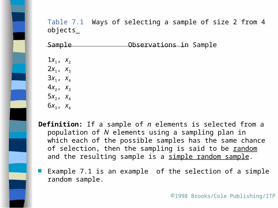
Table 7.1 Ways of selecting a sample of size 2 from 4 objects

Sample Observations in Sample

1 x1, x2

2 x1, x3 3 x1, x4

4 x2, x3 5 x2, x4

6 x3, x4

Definition: If a sample of n elements is selected from a population of N elements using a sampling plan in which each of the possible samples has the same chance of selection, then the sampling is said to be random and the resulting sample is a simple random sample.

Example 7.1 is an example of the selection of a simple random sample.


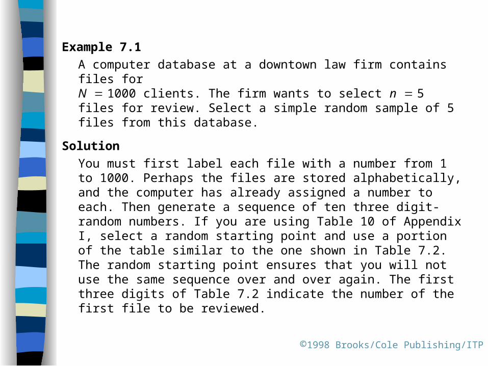
Example 7.1

A computer database at a downtown law firm contains files forN 1000 clients. The firm wants to select n 5 files for review. Select a simple random sample of 5 files from this database.

Solution

You must first label each file with a number from 1 to 1000. Perhaps the files are stored alphabetically, and the computer has already assigned a number to each. Then generate a sequence of ten three digit-random numbers. If you are using Table 10 of Appendix I, select a random starting point and use a portion of the table similar to the one shown in Table 7.2. The random starting point ensures that you will not use the same sequence over and over again. The first three digits of Table 7.2 indicate the number of the first file to be reviewed.


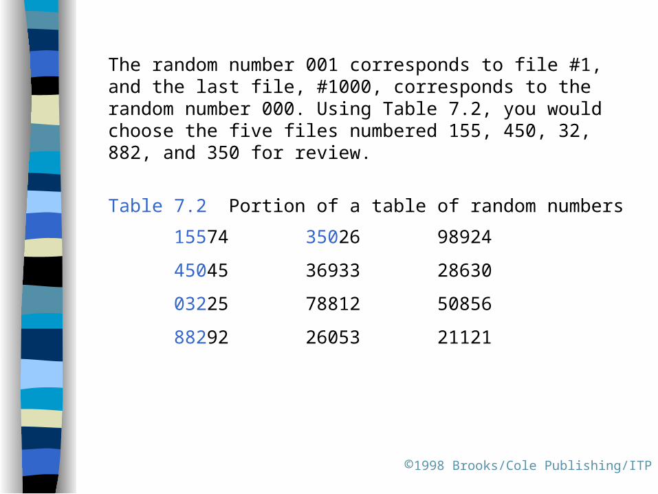
The random number 001 corresponds to file #1, and the last file, #1000, corresponds to the random number 000. Using Table 7.2, you would choose the five files numbered 155, 450, 32, 882, and 350 for review.

Table 7.2 Portion of a table of random numbers

15574 35026 98924

45045 36933 28630

03225 78812 50856

88292 26053 21121


A simple and reliable method of sampling uses random numbers—digits generated so that the values 0 to 9 occur randomly and with equal frequency.

Observational study: The data already existed before you decided to observe or describe their characteristics.

You must be careful when conducting a sample survey to watch for these problems:

- Nonresponse: Are the respondes you received biased because only certain subjects responded?

- Undercoverage: Does the database you used systematically exclude certain segments of the population?

- Wording bias: Question may be too complicated or tend to confuse.

Some research involves experimentation in which an experi-mental condition or treatment is imposed on the experimental units.


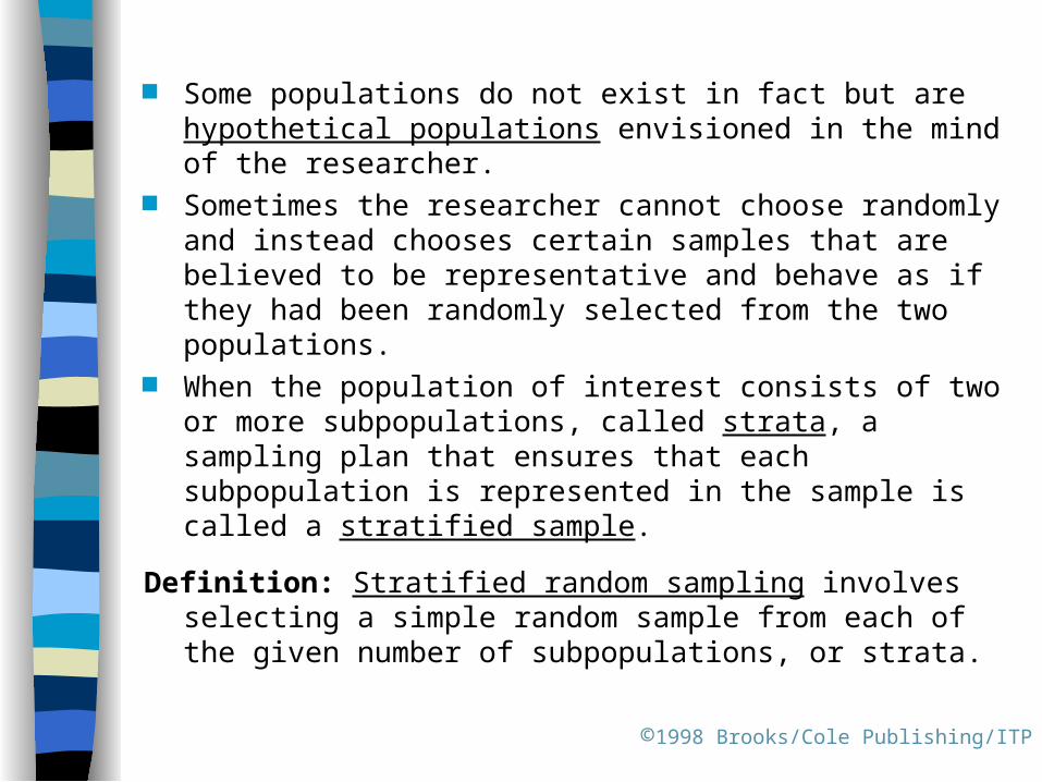
Some populations do not exist in fact but are hypothetical populations envisioned in the mind of the researcher.

Sometimes the researcher cannot choose randomly and instead chooses certain samples that are believed to be representative and behave as if they had been randomly selected from the two populations.

When the population of interest consists of two or more subpopulations, called strata, a sampling plan that ensures that each subpopulation is represented in the sample is called a stratified sample.

Definition: Stratified random sampling involves selecting a simple random sample from each of the given number of subpopulations, or strata.


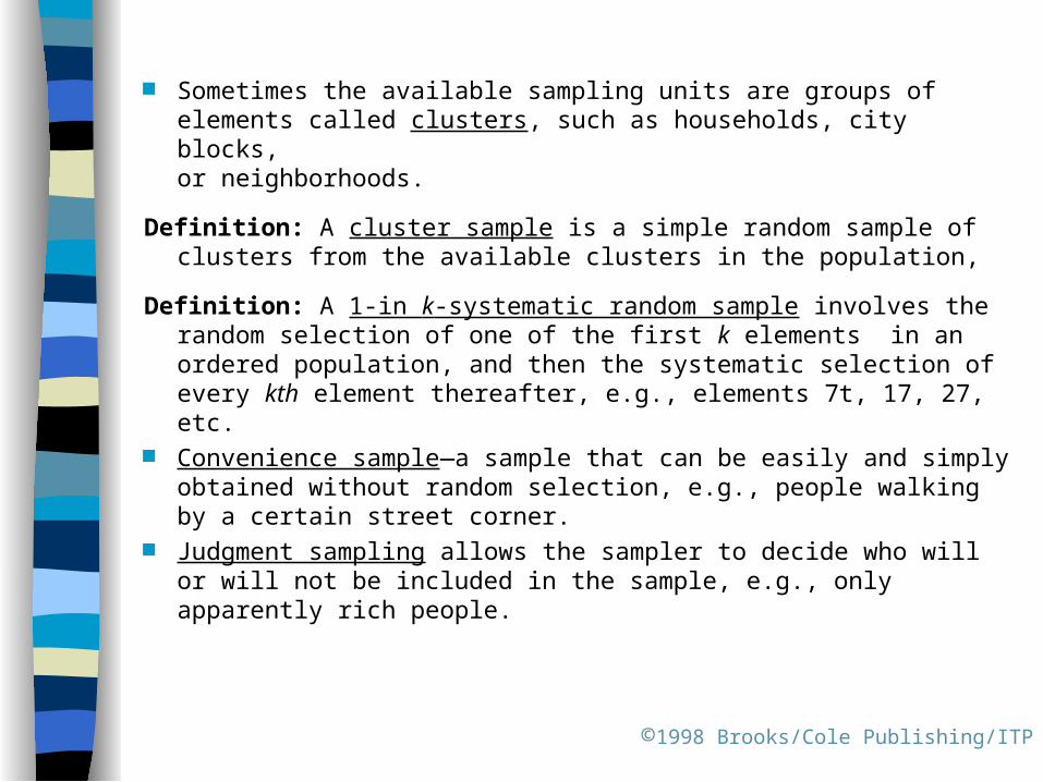
Sometimes the available sampling units are groups of elements called clusters, such as households, city blocks, or neighborhoods.

Definition: A cluster sample is a simple random sample of clusters from the available clusters in the population,

Definition: A 1-in k-systematic random sample involves the random selection of one of the first k elements in an ordered population, and then the systematic selection of every kth element thereafter, e.g., elements 7t, 17, 27, etc.

Convenience sample—a sample that can be easily and simply obtained without random selection, e.g., people walking by a certain street corner.

Judgment sampling allows the sampler to decide who will or will not be included in the sample, e.g., only apparently rich people.


Quota sampling—the makeup of the sample must reflect the makeup of the population on some selected characteristic, e.g., 90% white and 10% black, since that is the proportion in the total population.

Nonrandom samples can be described but cannot be used for making inferences.


7.3 Statistics and Sampling Distributions

The numerical descriptive measures you calculate from the sample are called statistics.

Statistics are random variables. The probability distributions for statistics are called sampling

distributions. In repeated sampling, they tell us what values of the statistics

can occur and how often each value occurs.

Definition: The sampling distribution of a statistic is the probability distribution for the possible values of the statistic that results when random samples of size n are repeatedly drawn from the population.


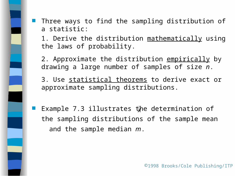
Three ways to find the sampling distribution of a statistic:

1. Derive the distribution mathematically using the laws of probability.

2. Approximate the distribution empirically by drawing a large number of samples of size n.

3. Use statistical theorems to derive exact or approximate sampling distributions.

Example 7.3 illustrates the determination of the sampling

distributions of the sample mean and the sample median m.


x

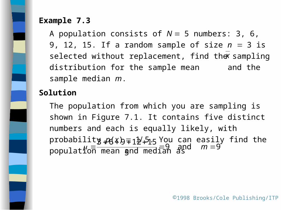
Example 7.3

A population consists of N 5 numbers: 3, 6, 9, 12, 15. If a

random sample of size n 3 is selected without replacement,

find the sampling distribution for the sample mean and the

sample median m.

Solution

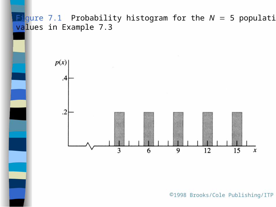
The population from which you are sampling is shown in Figure

7.1. It contains five distinct numbers and each is equally likely,

with probability p(x) 1 5. You can easily find the population

mean and median as


9 and 95

1512963 m

x


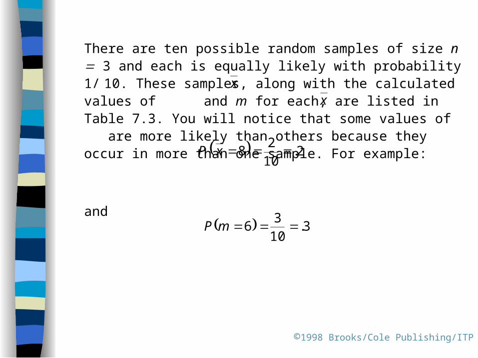
There are ten possible random samples of size n 3 and each is equally likely with probability 1/ 10. These samples, along with the calculated values of and m for each, are listed in Table 7.3. You will notice that some values of are more likely than others because they occur in more than one sample. For example:

and

2.102

8 xP

3.103

6 mP

xx


Figure 7.1 Probability histogram for the N 5 population values in Example 7.3


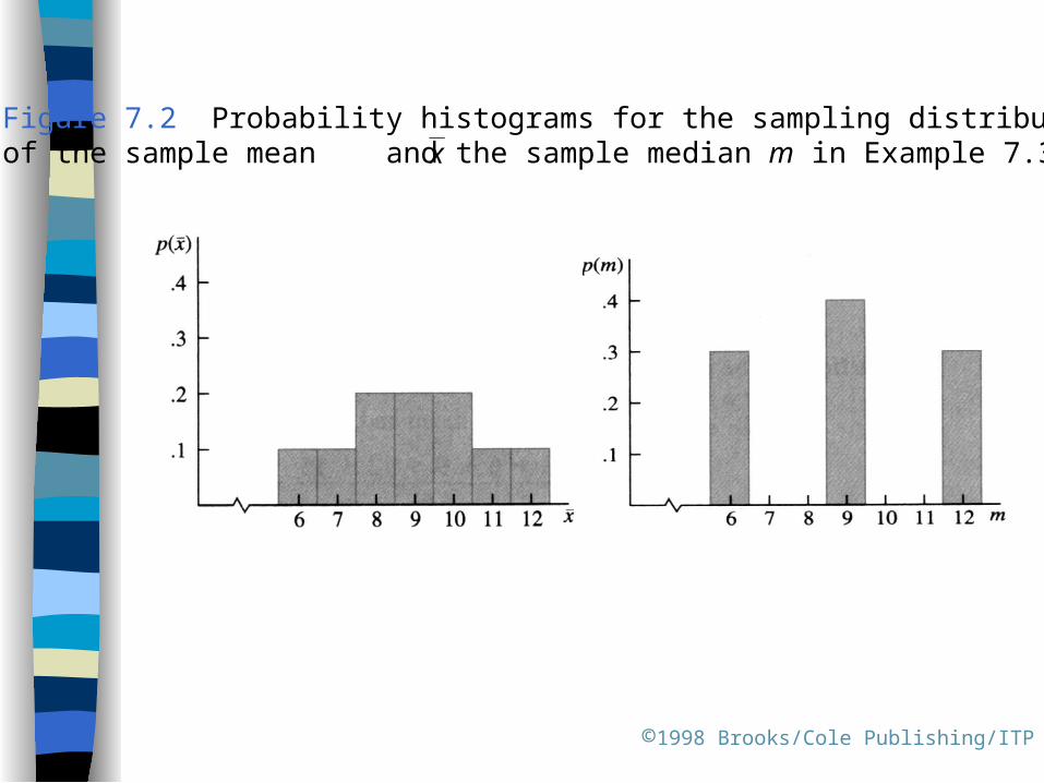
Figure 7.2 Probability histograms for the sampling distributions of the sample mean and the sample median m in Example 7.3x

When the number of elements in the population is very small, it is easy to derive the sampling distributions. Otherwise, you may need to use on of these methods:

- Approximate the sampling distribution empirically.

- Rely on statistical theorems and theoretical results.


7.4 The Central Limit Theorem

The Central Limit Theorem states that, under rather general conditions, sums and means of random samples of measure-ments drawn from a population tend to possess an approxi-mately normal distribution.

Figure 7.3 shows the probability distribution of the number appearing on a single toss of a die. Table 7.5 sums the upper faces of two dice.

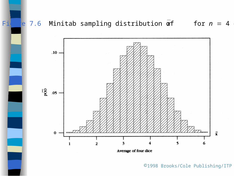
Figures 7.4 –7.6 illustrate the sampling distributions of for n 2, 3, 4, respectively.


x


Figure 7.3 Probability distribution for x, the number appearing on a single toss of a die

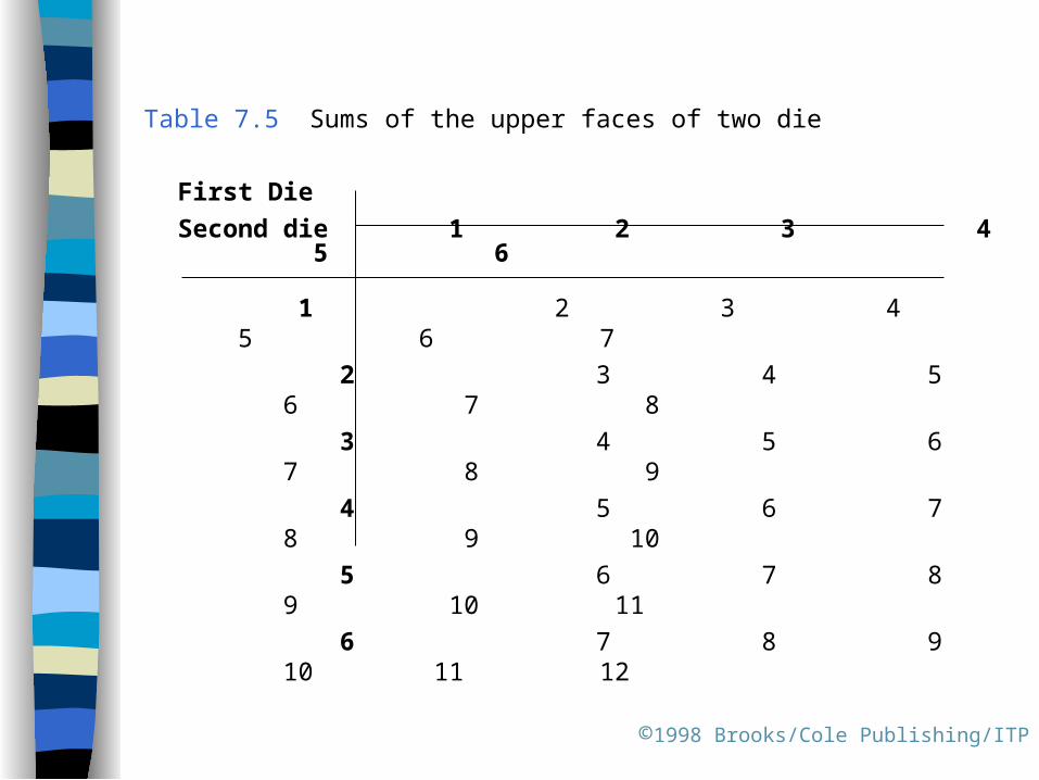
Table 7.5 Sums of the upper faces of two die

First Die

Second die 1 2 3 4 5 6

1 2 3 4 5 6 7

2 3 4 5 6 7 8

3 4 5 6 7 8 9

4 5 6 7 8 9 10

5 6 7 8 9 10 11

6 7 8 9 10 11 12



Figure 7.4 Sampling distribution of for n 2 dicex


Figure 7.5 Minitab sampling distribution of for n 3 dicex


Figure 7.6 Minitab sampling distribution of for n 4 dicex

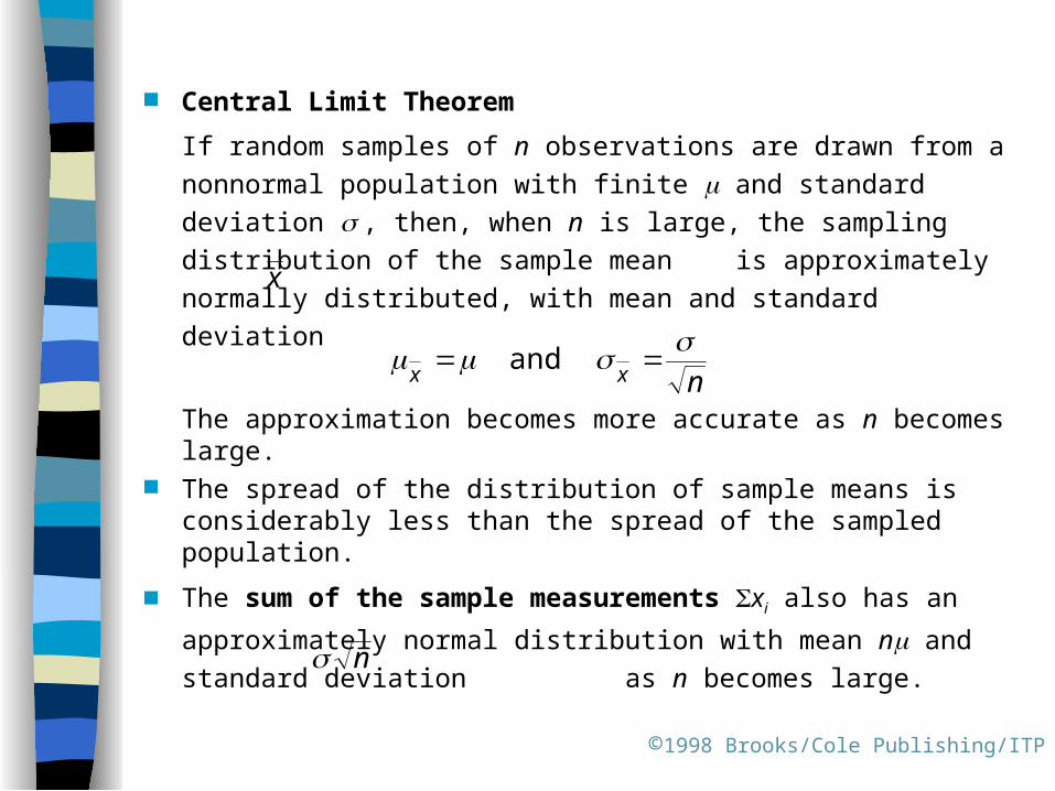
Central Limit Theorem

If random samples of n observations are drawn from a

nonnormal population with finite and standard deviation ,

then, when n is large, the sampling distribution of the sample

mean is approximately normally distributed, with mean and

standard deviation

The approximation becomes more accurate as n becomes large.

The spread of the distribution of sample means is considerably less than the spread of the sampled population.

The sum of the sample measurements xi also has an

approximately normal distribution with mean n and standard

deviation as n becomes large.


x

nxx

and

n

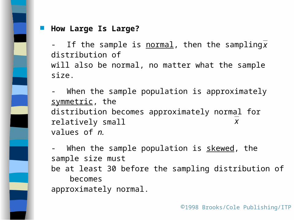
How Large Is Large?

- If the sample is normal, then the sampling distribution of will also be normal, no matter what the sample size.

- When the sample population is approximately symmetric, the

distribution becomes approximately normal for relatively small

values of n.

- When the sample population is skewed, the sample size must

be at least 30 before the sampling distribution of becomes

approximately normal.


x

x

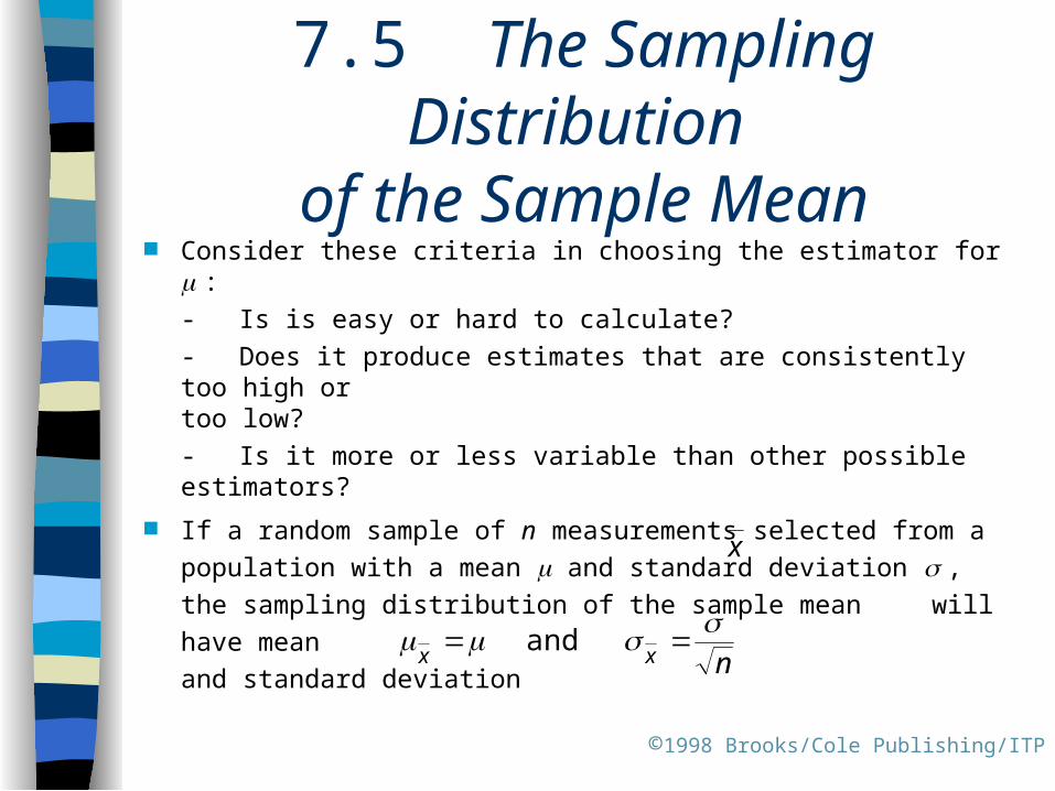
7.5 The Sampling Distribution of the Sample Mean

Consider these criteria in choosing the estimator for :

- Is is easy or hard to calculate?

- Does it produce estimates that are consistently too high or too low?

- Is it more or less variable than other possible estimators?

If a random sample of n measurements selected from a

population with a mean and standard deviation , the

sampling distribution of the sample mean will have mean

and standard deviation


x

n

xx

and

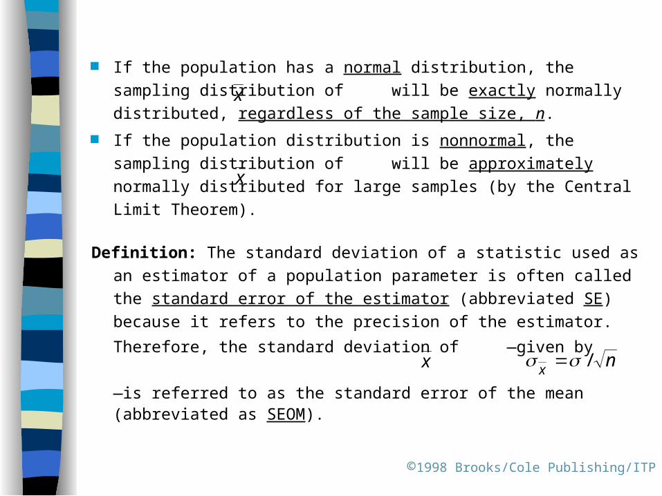
If the population has a normal distribution, the sampling

distribution of will be exactly normally distributed, regardless

of the sample size, n.

If the population distribution is nonnormal, the sampling

distribution of will be approximately normally distributed for

large samples (by the Central Limit Theorem).

Definition: The standard deviation of a statistic used as an

estimator of a population parameter is often called the standard

error of the estimator (abbreviated SE) because it refers to the

precision of the estimator.

Therefore, the standard deviation of —given by

—is referred to as the standard error of the mean (abbreviated as SEOM).


x

nx

/

x

x

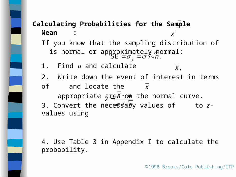
Calculating Probabilities for the Sample Mean :

If you know that the sampling distribution of is normal or approximately normal:

1. Find and calculate

2. Write down the event of interest in terms of and locate

the

appropriate area on the normal curve.

3. Convert the necessary values of to z-values using

4. Use Table 3 in Appendix I to calculate the probability.


./SE nx

n

xz

/

x

x

,x

x

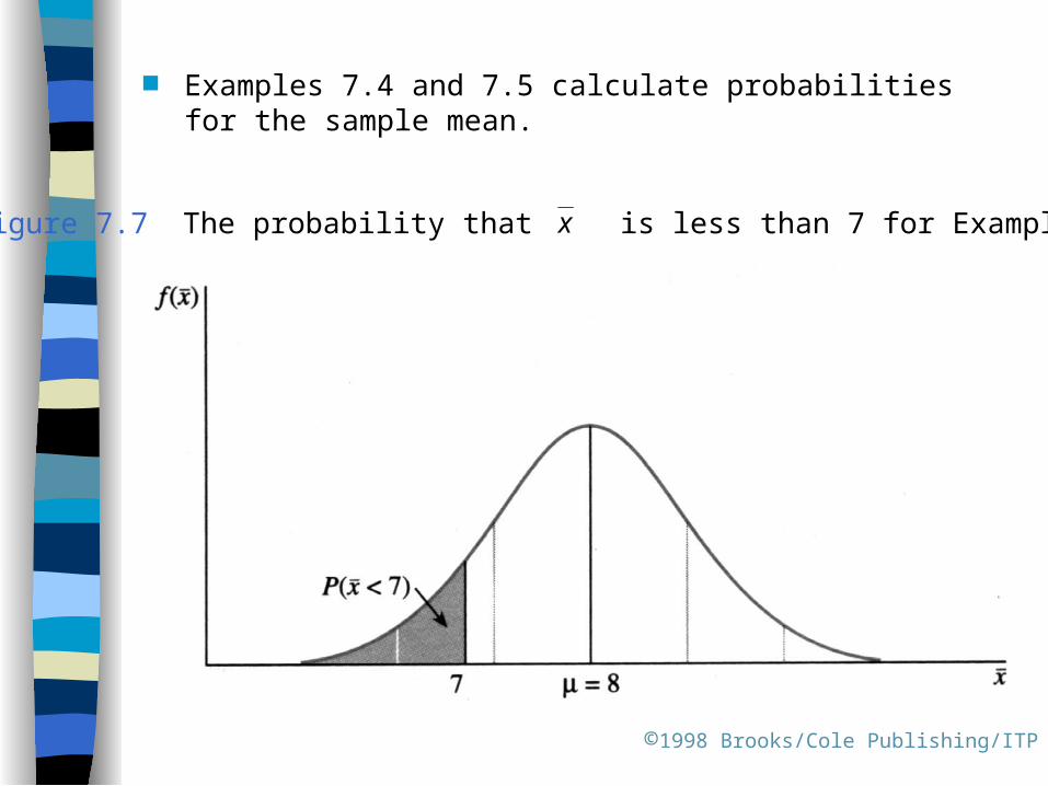
Examples 7.4 and 7.5 calculate probabilities for the sample mean.


Figure 7.7 The probability that is less than 7 for Example 7.4x


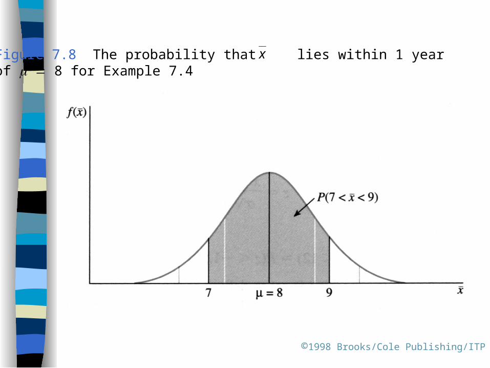
Figure 7.8 The probability that lies within 1 year of 8 for Example 7.4

x

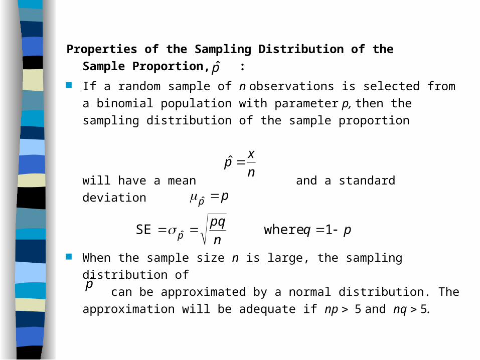
Properties of the Sampling Distribution of the

Sample Proportion, :

If a random sample of n observations is selected from a

binomial population with parameter p, then the sampling

distribution of the sample proportion

will have a mean and a standard deviation

When the sample size n is large, the sampling distribution of

can be approximated by a normal distribution. The

approximation will be adequate if np 5 and nq 5.

p̂

nx

p ˆ

pp ˆ

pqnpq

p 1 where SE ˆ

p̂

Example 7.6 deals with the sampling distribution of the sample proportion

Example 7.6

In a survey, 500 mothers and fathers were asked about the importance of sports for boys and girls. Of the parents interviewed, 60% agreed that the genders are equal and should have equal opportunities to participate in sports. Describe the sampling distribution of the sample proportion of parents who agree that the genders are equal and should have equal opportunities.

Solution

You can assume that the 500 parents represent a random sample of the parents of all boys and girls in the United States and that the true proportion in the population is equal to some unknown value that you can call p.


.p̂

p̂

The sampling distribution of can be approximated by a normal distribution with mean equal to p (see Figure 7.10) and standard deviation

Calculating Probabilities for the Sample Proportion :

1. Find the necessary values of n and p.

2. Check whether the normal approximation to the binomial distribution is appropriate (np 5 and nq 5).

3. Write down the event of interest in terms of and locate the appropriate area on the normal curve.

4. Convert the necessary values of to z-values using

5. Use Table 3 in Appendix I to calculate the probability.

Example 7.7 deals with the probability of observing a certain sample proportion.


npqppz //ˆ

npq

p ˆSE

p̂

p̂

p̂

p̂

7.7 A Sampling Application: Statistical Process Control

(Optional)

The cause of a change in the variable is said to be assignable if it can be found and corrected.

Other variation that is not controlled is regarded as random variation.

If the variation in a process variable is solely random, the process is said to be in control.

If out of control, we must reduce the variation and get themeasurements of the process variable within specified limits.

Example 7.8 requires the construction of an chart for monitoring the process mean.


x

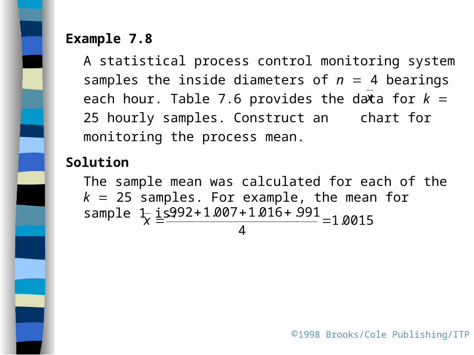
Example 7.8

A statistical process control monitoring system samples the

inside diameters of n 4 bearings each hour. Table 7.6

provides the data for k 25 hourly samples. Construct an

chart for monitoring the process mean.

Solution

The sample mean was calculated for each of the k 25 samples. For example, the mean for sample 1 is:


0015.14

991.016.1007.1992.

x

x

Table 7.6 25 hourly samples of bearing diameters

Sample Sample Sample measurements mean,

1 .992 1.007 1.016 .991 1.00150

2 1.015 .984 .976 1.000 .993753 .988 .993 1.011 .981 .993254 .996 1.020 1.004 .999 1.004755 1.015 1.006 1.002 1.001 1.006006 1.000 .982 1.005 .989 .994007 .989 1.009 1.019 .994 1.002758 .994 1.010 1.009 .990 1.000759 1.018 1.016 .990 1.011 1.00875

10 .997 1.005 .989 1.001 .9980011 1.020 .986 1.002 .989 .9992512 1.007 .986 .981 .995 .9922513 1.016 1.002 1.010 .999 1.00675


x

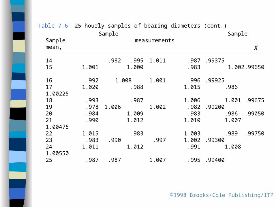
Table 7.6 25 hourly samples of bearing diameters (cont.)

Sample Sample Sample measurements mean,

14 .982 .995 1.011 .987 .9937515 1.001 1.000 .983 1.002 .9965016 .992 1.008 1.001 .996 .99925 17 1.020 .988 1.015 .986 1.0022518 .993 .987 1.006 1.001 .99675 19 .978 1.006 1.002 .982 .9920020 .984 1.009 .983 .986 .9905021 .990 1.012 1.010 1.007 1.0047522 1.015 .983 1.003 .989 .9975023 .983 .990 .997 1.002 .9930024 1.011 1.012 .991 1.008 1.0055025 .987 .987 1.007 .995 .99400


x

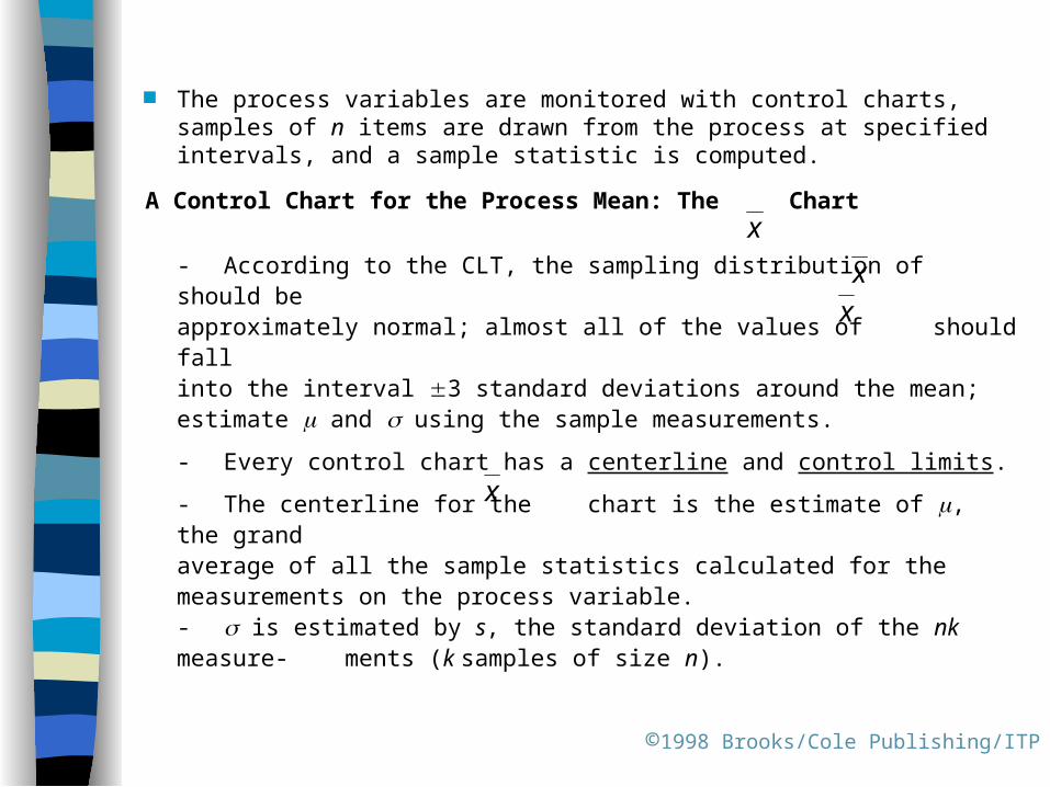
The process variables are monitored with control charts, samples of n items are drawn from the process at specified intervals, and a sample statistic is computed.

A Control Chart for the Process Mean: The Chart

- According to the CLT, the sampling distribution of should be

approximately normal; almost all of the values of should fall into the interval 3 standard deviations around the mean; estimate and using the sample measurements.

- Every control chart has a centerline and control limits.

- The centerline for the chart is the estimate of , the grandaverage of all the sample statistics calculated for themeasurements on the process variable.

- is estimated by s, the standard deviation of the nk measure-ments (k samples of size n).


x

xx

x

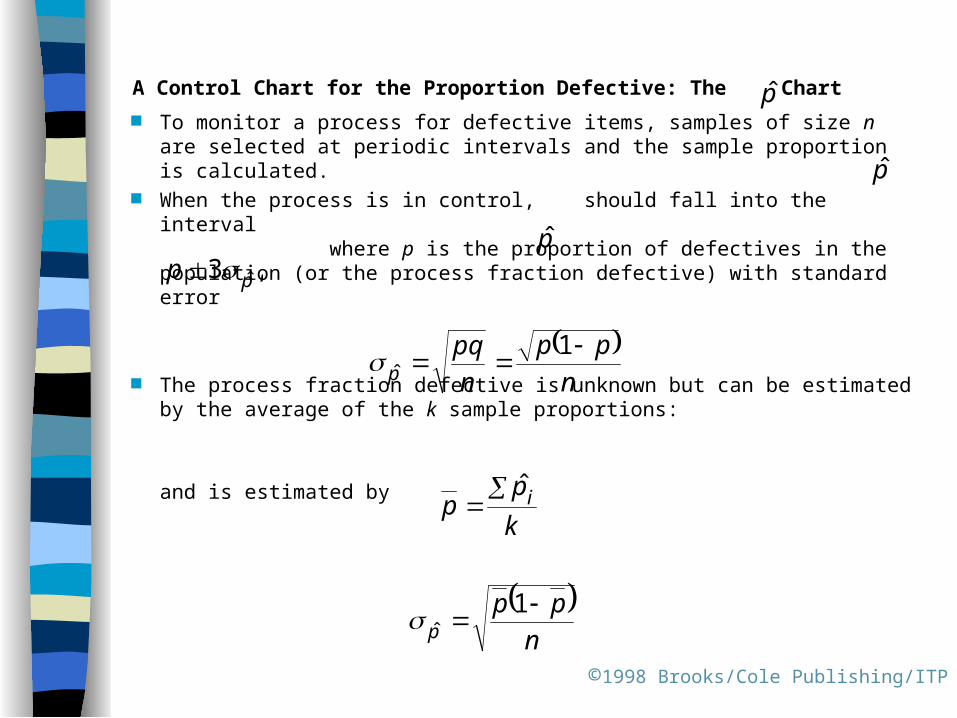
A Control Chart for the Proportion Defective: The Chart

To monitor a process for defective items, samples of size n are selected at periodic intervals and the sample proportion is calculated.

When the process is in control, should fall into the interval where p is the proportion of defectives in the population (or the process fraction defective) with standard error

The process fraction defective is unknown but can be estimated by the average of the k sample proportions:

and is estimated by


p̂

k

pp i

ˆ

n

ppp

1ˆ

,3 p̂p

n

pp

npq

p

1

ˆ

p̂

p̂

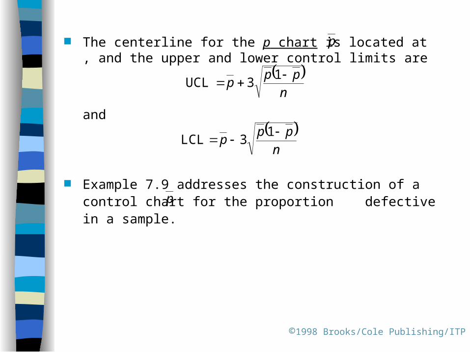
The centerline for the p chart is located at , and the upper and lower control limits are

and

Example 7.9 addresses the construction of a control chart for the proportion defective in a sample.


p

n

ppp

13UCL

p

n

ppp

13LCL

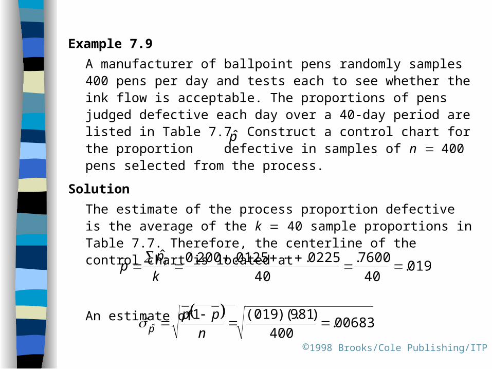
Example 7.9

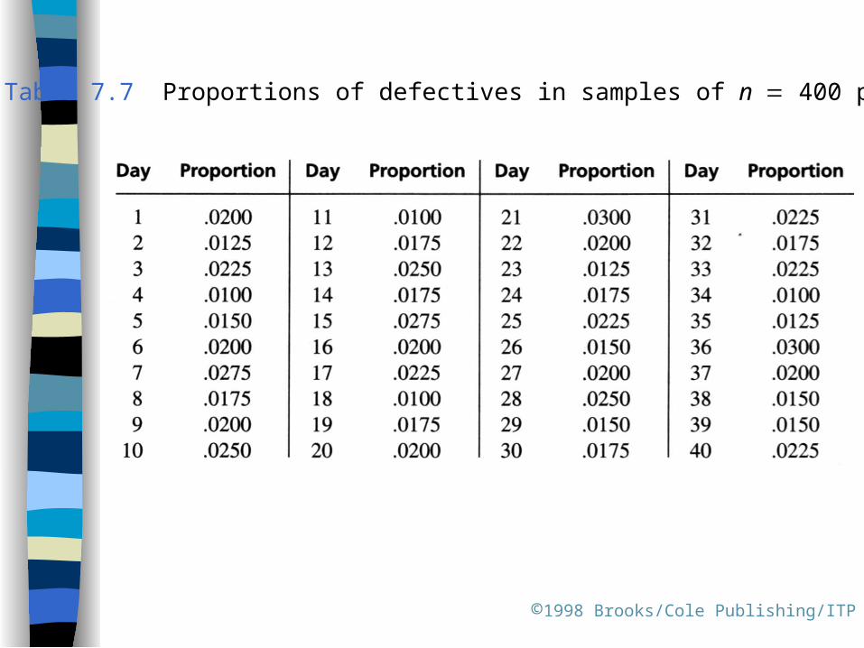
A manufacturer of ballpoint pens randomly samples 400 pens per day and tests each to see whether the ink flow is acceptable. The proportions of pens judged defective each day over a 40-day period are listed in Table 7.7. Construct a control chart for the proportion defective in samples of n 400 pens selected from the process.

Solution

The estimate of the process proportion defective is the average of the k 40 sample proportions in Table 7.7. Therefore, the centerline of the control chart is located at

An estimate of


019.40

7600.40

0225.0125.200.0ˆ

k

pp i

00683.

400)981)(.019(.1

ˆ ˆ n

ppp

p̂

and Therefore, the upper and lower

control limits for the chart are located at

and

Or, since p cannot be negative, LCL 0.

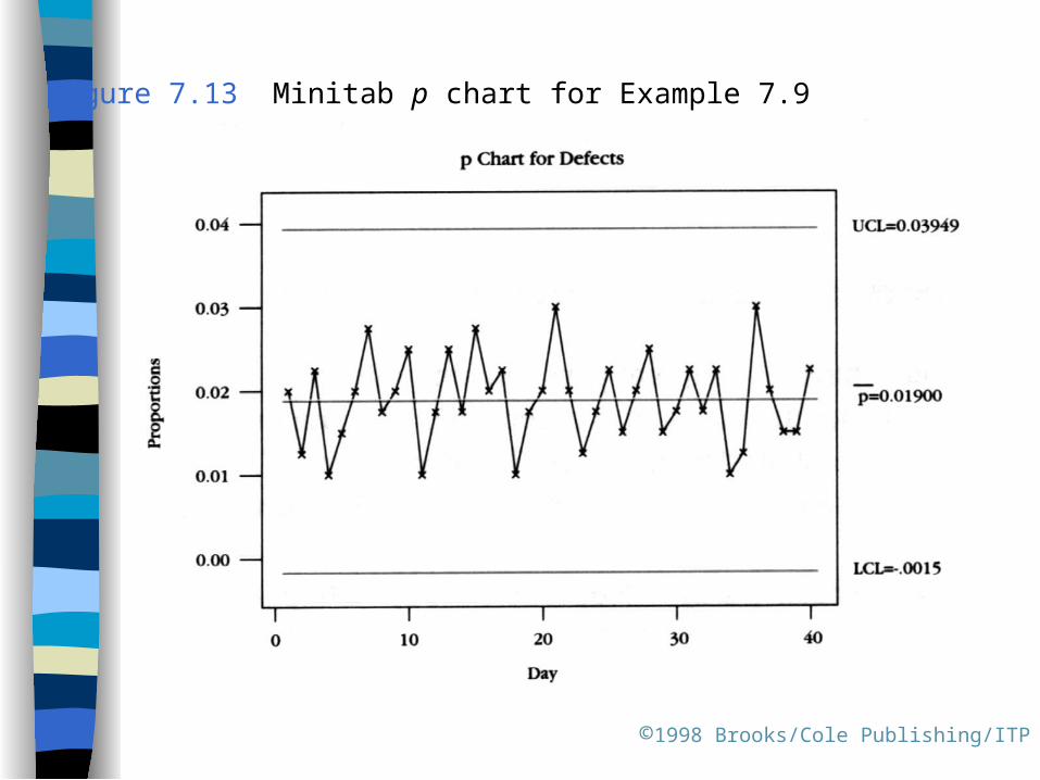
The p control chart is shown in Figure 7.13. Note that all 40 sample proportions fall within the control limits. If a sample proportion collected at some time in the future falls outside the control limits, the manufacturer will be warned of a possible increase in the value of the process proportion defective. Efforts will be initiated to seek possible causes for an increase in the value of the process proportion defective.


.0205.)00683)(.3(ˆ3 ˆ p

0395.0205.0190.ˆ3UCL ˆ pp

0015.0205.0190.ˆ3LCL ˆ pp


Table 7.7 Proportions of defectives in samples of n 400 pens


Figure 7.13 Minitab p chart for Example 7.9

Other commonly used control charts are the R chart, which is used to monitor variation In the process variable by using the sample range, and the c chart, which is used to monitor the number of defects per item.


Key Concepts and Formulas

I. Sampling Plans and Experimental Designs

1. Simple random sampling

a. Each possible sample is equally likely to occur.

b. Use a computer or a table of random numbers.

c. Problems are nonresponse, undercoverage, and wording bias.

2. Other sampling plans involving randomization

a. Stratified random sampling

b. Cluster sampling

c. Systematic 1-in-k sampling


3. Nonrandom sampling

a. Convenience sampling

b. Judgment sampling

c. Quota sampling

II. Statistics and Sampling Distributions

1. Sampling distributions describe the possible values of a statistic and how often they occur in repeated sampling.

2. Sampling distributions can be derived mathematically,approximated empirically, or found using statistical

theorems.

3. The Central Limit Theorem states that sums and averages of

measurements from a nonnormal population with finite mean

and standard deviation have approximately normal distributions for large samples of size n.


III. Sampling Distribution of the Sample Mean

1. When samples of size n are drawn from a normal population

with mean and variance 2, the sample mean has a normal distribution with mean and variance 2n.

2. When samples of size n are drawn from a nonnormal population with mean and variance 2, the Central Limit

Theorem ensures that the sample mean will have an approximately normal distribution with mean and

variance2n when n is large (n 30).

3. Probabilities involving the sample mean can be

calculated

by standardizing the value of using z:


x

n

xz

/

x

x

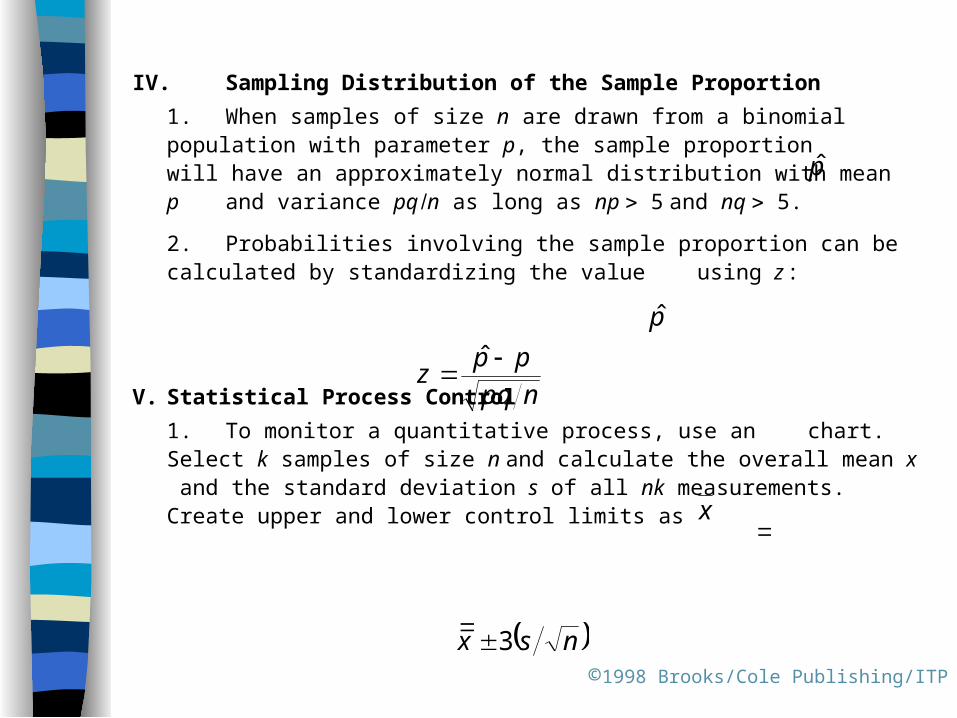
IV. Sampling Distribution of the Sample Proportion

1. When samples of size n are drawn from a binomial population with parameter p, the sample proportion will have an approximately normal distribution with mean p and variance pq n as long as np 5 and nq 5.

2. Probabilities involving the sample proportion can be calculated by standardizing the value using z :

V. Statistical Process Control

1. To monitor a quantitative process, use an chart. Select k samples of size n and calculate the overall mean x and the standard deviation s of all nk measurements. Create upper and lower control limits as


p̂

npq

ppz

ˆ

nsx 3

p̂

x

If a sample mean exceeds these limits, the process is out of

control.

2. To monitor a binomial process, use a p chart. Select k samples of size n and calculate the average of the sample proportions as

Create upper and lower control limits as

If a sample proportion exceeds these limits, the process is out of control.


k

pp i

ˆ

n

ppp

13

Documents

Chapter 7 Sampling Distributions General Objectives: We begin to study samples and the statistics that describe them. These samples statistics are used