Chapter 7. Functions of Random Variables

The UNIVERSITY of NORTH CAROLINA at CHAPEL HILL

Chapter 7. Functions of Random Variables

Sections 7.2 -- 7.4: Functions of Discrete Random Variables, Method of Distribution Functions and Method of Transformations in One Dimension

Jiaping Wang

Department of Mathematical Science

04/10/2013, Wednesday


Outline Functions of Discrete Random Variables Methods of Distribution Functions Method of Transformations in One Dimension More Examples Homework #10


Part 1. Functions of Discrete Random Variables


Introduction

For example, there is a sample X1, X2, …, Xn from same distribution, also there is a function denoted by Y=f(X1, X2, …, Xn)=1/n∑Xi, which is a function of random variables {X1, X2, …, Xn}. Considering the discrete random variables, for example, X is a discrete random variables with space S={0, 1, 2, 3}, C is a function of X with C=150+50X, then we can have a mass probability table x 0 1 2 3

p(x) 0.5 0.3 0.15 0.05

c 150 200 250 300

p(c) 0.5 0.3 0.15 0.05


Cont.

Considering X is a discrete random variables with space S={-1, 0, 1}, define Y=X2, then we can have a mass probability table as follows

x -1 0 1

p(x) 0.25 0.5 0.25

y 1 0 1

p(y) 0.25 0.5 0.25

y 0 1

p(y) 0.5 0.5


Example 7.1

A quality control manager samples from a lot of items, testing each item until r defectives have been found. Find the distribution of Y, the number of items that are tested to obtain r defectives.

Answer: Assume that the probability p of obtaining a defective item is constant from trial To trial, the number of good items X sampled prior to the r-th defective one is a negative Binomial random variable. The mass function is 𝑃 𝑋 = 𝑥 = 𝑝 𝑥 = 𝑥+𝑟−1

𝑟−1 𝑝𝑟𝑞𝑥, 𝑥 = 0, 1, 2, … The number of trials, Y, is equal to the sum of the number of good items and defective Ones, that is, Y=X+r thus X=Y-r, with Y=r, r+1, r+2, … so the mass function for Y is 𝑃 𝑌 = 𝑦 = 𝑝 𝑦 = 𝑦−1

𝑟−1 𝑝𝑟𝑞𝑦 − 𝑟, 𝑦 = 𝑟, 𝑟 + 1, 𝑟 + 2, …


Part 2. Method of Distribution Functions


Introduction

If X has a probability density function 𝒇𝑿(𝒙), and Y is a function of X, we are interested in finding 𝑭𝒀(𝒚) = 𝑷(𝒀 ≤𝒚) or the density 𝒇𝒀(𝒚) by using the distribution of X. For example, 𝒀 = 𝑿𝟐 with density 𝒇𝑿(𝒙). For y≥0, 𝑭𝒀 𝒚 = 𝑷 𝒀 ≤ 𝒚 = 𝑷 𝑿𝟐 ≤ 𝒚 = 𝑷 − 𝒚 ≤ 𝑿 ≤ 𝒚 = 𝑷 𝑿 ≤ 𝒚 − 𝐏 𝐗 ≤ − 𝒚 = 𝑭𝑿 𝒚 − 𝑭𝑿 − 𝒚 . Then we can have the density function for Y: 𝒇𝒀 𝒚 = 𝒅

𝒅𝒚𝑭𝒀 𝒚 = 𝒅

𝒅𝒚𝑭𝑿 𝒚 − 𝒅

𝒅𝒚𝑭𝑿 − 𝒚

=𝟏

𝟐 𝒚𝒇𝑿 𝒚 +

𝟏𝟐 𝒚

𝒇𝑿 − 𝒚


Application in Normal Distribution

X is standard normal random variable, what is the probability density function of Y=X2? We know 𝑓𝑋 𝑥 = 1

2𝜋exp −𝑥2

2,−∞ < 𝑥 < ∞, thus for y≥0,

𝑓𝑌 𝑦 = 1

2 𝑦[ 12𝜋

exp − ( 𝑦)2

2+ 1

2𝜋exp − (− 𝑦)2

2] = 1

2 𝜋y − 1

2 exp(−y2)

Recall that Γ 1

2= 𝜋, we can see Y follows a gamma distribution with

parameters α=1/2 and β=2.


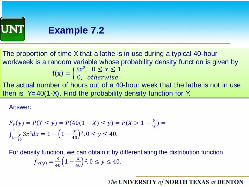
Answer: 𝐹𝑌(𝑦) = 𝑃(𝑌 ≤ 𝑦) = 𝑃(40(1 − 𝑋) ≤ 𝑦) = 𝑃(𝑋 > 1 − 𝑦

40) =

∫ 3𝑥2𝑑𝑥 = 1 − 1 − 𝑥40

3, 0 ≤ 𝑦 ≤ 40.11− 𝑦

40

For density function, we can obtain it by differentiating the distribution function 𝑓𝑌 𝑦 = 3

401 − x

402, 0 ≤ 𝑦 ≤ 40.

The proportion of time X that a lathe is in use during a typical 40-hour workweek is a random variable whose probability density function is given by

f x = �3𝑥2, 0 ≤ 𝑥 ≤ 1

0, 𝑜𝑜𝑜𝑜𝑟𝑜𝑜𝑜𝑜.

The actual number of hours out of a 40-hour week that the lathe is not in use then is Y=40(1-X). Find the probability density function for Y.

Example 7.2


Example 7.5

Let X have the probability density function given by

𝑓 𝑥 = �𝑥 + 1

2, −1 ≤ 𝑥 ≤ 1

0, 𝑜𝑜𝑜𝑜𝑟𝑜𝑜𝑜𝑜

Find the density function for Y=X2.

Answer: In the earlier section, we found that

𝒇𝒀 𝒚 =𝟏

𝟐 𝒚 [𝒇𝑿 𝒚 + 𝒇𝑿 − 𝒚 ]

By substituting into this equation, we have

𝒇𝒀 𝒚 = 𝟏𝟐 𝒚

𝒚+𝟏𝟐

+ − 𝒚+𝟏𝟐

= �𝟏𝟐 𝒚

, 𝟎 ≤ 𝒚 ≤ 𝟏

𝟎, 𝒐𝒐𝒐𝒐𝒐𝒐𝒐𝒐𝒐

As −𝟏 ≤ 𝒙 ≤ 𝟏,𝒚 = 𝒙𝟐 𝟎 ≤ 𝒚 ≤ 𝟏


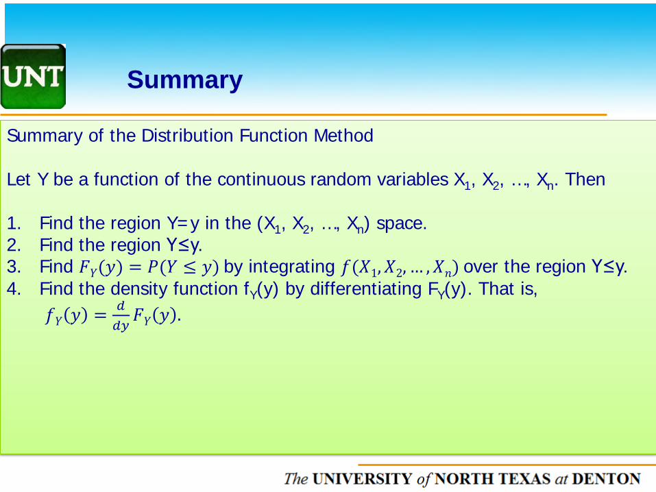
Summary

Summary of the Distribution Function Method Let Y be a function of the continuous random variables X1, X2, …, Xn. Then 1. Find the region Y=y in the (X1, X2, …, Xn) space. 2. Find the region Y≤y. 3. Find 𝐹𝑌(𝑦) = 𝑃(𝑌 ≤ 𝑦) by integrating 𝑓(𝑋1,𝑋2, … ,𝑋𝑛) over the region Y≤y. 4. Find the density function fY(y) by differentiating FY(y). That is,

𝑓𝑌 𝑦 = 𝑑𝑑𝑦𝐹𝑌 𝑦 .


Part 3. Method of Transformation in One Dimension


Introduction

The transformation method for finding the probability distribution of a function of a random variable is simply a generalization of the distribution function method. Consider a random variable X with the distribution function FX(x). Suppose that Y is a function of X, say, Y=g(X) which is an increasing function with the inverse X=g-1(Y)=h(Y). Then We have 𝐹𝑌 𝑦 = 𝑃 𝑌 ≤ 𝑦 = 𝑃 𝑔 𝑋 ≤ 𝑦 = 𝑃 𝑋 ≤ 𝑜 𝑦 = 𝐹𝑋[𝑜 𝑦 ] Then the density function is 𝑓𝑌 𝑦 = 𝑑

𝑑𝑦𝐹𝑌 𝑦 = 𝑑

𝑑𝑦𝐹𝑋 𝑜 𝑦 = 𝑓𝑋 𝑜 𝑦 ∙ |𝑜′ 𝑦 |.

Similarly, we can have the same result for g(X) is a decreasing function.


Theorem 7.1

Transformation of Random Variable. Let X be an absolute continuous random variable with probability density function

𝑓𝑋 𝑥 = �> 0, 𝑥 ∈ 𝐴 = (𝑎, 𝑏)

0, 𝑥 ∈ �̅�

Let 𝑌 = 𝑔(𝑋) with inverse function 𝑋 = 𝑜(𝑌) such that h is a one-to-one, continuous function from 𝐵 = (𝛼,𝛽) onto A. If 𝑜’(𝑦) exists and 𝑜’(𝑦) ≠ 0 for all y ∈ 𝐵. Then 𝑌 = 𝑔(𝑋) determines a new random variable with density

𝑓𝑌 𝑦 = �𝑓𝑋 𝑜 𝑦 |𝑜′ 𝑦 |, 𝑦 ∈ 𝐵 = (𝛼,𝛽)

0, 𝑦 ∈ 𝐵�


Example 7.6

Let X have the probability density function given by

𝑓 𝑥 = �2𝑥, 0 ≤ 𝑥 ≤ 10, 𝑜𝑜𝑜𝑜𝑟𝑜𝑜𝑜𝑜

Find the density function for Y=-2X+5.

Answer: Here 𝑌 = 𝑔(𝑋) = −2𝑋 + 5 the inverse function 𝑋 = 𝑜 𝑌 = 5−𝑌2

where h is a continuous and one-to-one function from B=(3,5) onto A=(0,1). So 𝑜’(𝑦) = −1/2 for any y ∈ 𝐵 . Then we can have 𝑓𝑌 𝑦 = 𝑓𝑋 𝑜 𝑦 𝑜′ 𝑦 = 2 5−𝑦

2− 12

= 5−𝑦2

, 3 < 𝑦 < 5.


Summary

Summary of the Univariate Transformation Method Let Y be the function of the continuous random variables X, Y=g(X). Then 1. Write the probability density function of X. 2. Find the inverse function h such that X=h(Y). Verify that h is a continuous

one-to-tone function from B=(α, β) onto A=(a, b) where for 𝑥 ∈ 𝐴, 𝑓 𝑥 >0.

3. Verify 𝑑𝑑𝑦𝑜 𝑦 = 𝑜′(𝑦) exists, and is not zero for any 𝑦 ∈ 𝐵.

4. Find 𝑓𝑌(𝑦) by calculating 𝑓𝑋 𝑜 𝑦 |𝑜′ 𝑦 |


Part 4. Additional Examples


Additional Example 1

Let X be a random variable having a continuous c.d.f., F(x). Let Y=F(X). Show that Y has a uniform distribution on (0,1). Conversely, if U has a uniform distribution on (0,1), show that X = F-1(U) has the c.d.f, F(x).

Answer: F(X) is non-decreasing and has domain 0<F(X)<1, that is, 0<Y<1. Suppose F(x) has inverse function, ie., y=F(x)x=F-1(y). Then FY(y)=P(Y ≤ y)=P[F(X) ≤ y]=P[X ≤F-1(y)]=F(F-1(y))=y fY(y)=1, for 0<y<1. FX(x)=P(X ≤x)=P(F-1(U) ≤x)=P(U ≤F(x))=F(x).


Additional Example 2

Show that if U is uniform on (0,1), then X=-log(U) has an exponential distribution Exp(1).

Answer: The density function for U is fU(u)=1. X=-log(U) U=exp(-X), so h(x)=e-x, which is continuous and one-to-one function with B=(0, ∞) as A=(0, 1). The derivative of h(x) is h’(x)=-e-x which is not zero in the domain. So we can have fX(x) =fU[h(x)]|h’(x)|=(1)(|-e-x|)=e-x.


Homework #10

Page 275: 5.138, 5.140 Page 354: 7.3, 7.4 Page 362: 7.6, 7.8 Page 366: 7.18, 7.20 Due Monday, 04/22/2013

Documents

Chapter 7. Functions of Random Variables