Embed Size (px)
Citation preview
On the rational functions innon-commutative random variables
Dissertationzur Erlangung des Grades
des Doktors der Naturwissenschaftender Fakultat fur Mathematik und Informatik
der Universitat des Saarlandes
Sheng Yin
Saarbrucken, 2019
Datum der Verteidigung: 27. Januar 2020Dekan: Prof. Dr. Sebastian HackPrufungsausschuss: Vorsitzender:
Prof. Dr. Gabriela Weitze-SchmithsenBerichterstatter:
Prof. Dr. Roland SpeicherProf. Dr. Moritz WeberProf. Dr. Thomas Schick
Akademischer MitarbeiterDr. Marwa Banna
Abstract
This thesis is devoted to some problems on non-commutative rational functions in non-commutative random variables that come from free probability theory and from randommatrix theory.
First, we will consider the non-commutative random variables in tracialW ∗-probabilityspaces, such as freely independent semicircular and Haar unitary random variables. Anatural question on rational functions in these random variables is the well-definednessquestion. Namely, how large is the family of rational functions that have well-definedevaluations for a given tuple X of random variables? Note that for a fixed rationalfunction r, the well-definedness of its evaluation r(X) depends on the interpretation ofthe invertibility of random variables. This is because the invertibility of a random variablein a tracial W ∗-probability space (or an operator in a finite von Neumann algebra) canbe also considered in a larger algebra, i.e., the ∗-algebra of affiliated operators. Oneof our goals in this thesis to show some criteria that characterize the well-definednessof all rational functions in the framework of affiliated operators. In particular, one ofthese criteria is given by a homological-algebraic quantity on non-commutative randomvariables. We will also show that some notions provided by free probability are relatedto this quantity. So we can finally answer the well-definedness question via these relatednotions from free probability.
Those criteria for the well-definedness of rational functions are actually intrinsic con-nected to the Atiyah conjecture or Atiyah property. We will explore these connectionsbetween the Atiyah property and our question on the well-definedness of rational func-tions. In particular, we will present a result to show a connection between the so-calledstrong Atiyah property and the invertibility of evaluations of rational functions. In thisresult, the evaluation of a rational function at a tuple of random variables may not bewell-defined, but it is always invertible as an affiliated operator once it is well-defined.
In the last part of this thesis, we will turn to the questions on rational functions inrandom matrices. Besides the well-definedness problem for rational functions in randommatrices, we will also address the convergence problem for rational functions in randommatrices. Due to the unstableness of the convergence in distribution, we will limit our ran-dom matrices to the ones that strongly converge in distribution and our rational functionsto the ones that have bounded evaluations. We will show that both the well-definenessand the convergence problem have an affirmative answer under such conditions.
i

Abstrakt
Diese Doktorarbeit widmet sich Problemen aus der freien Wahrscheinlichkeitstheorieund der Zufallsmatrizentheorie uber nicht-kommutative rationale Funktionen in nicht-kommutativen Zufallsvariablen.
Zunachst betrachten wir nicht-kommutative Zufallsvariable in endlichen (d.h. tra-cial) W ∗-Wahrscheinlichkeitsraumen, wie z.B. freie Halbkreiselemente oder freie Haarunitare Zufallsvariable. Eine naturliche Frage uber rationale Funktionen in solchen Zu-fallsvariablen ist die nach der Wohldefiniertheit. Genauer gesagt, wie groß ist die Familievon rationalen Funktionen, die eine wohldefinierte Auswertung fur ein gegebenes Tu-pel X von Zufallsvariablen haben? Man muss beachten, dass fur eine feste rationaleFunktion r die Wohldefiniertheit der Auswertung r(X) von der Interpretation der In-vertierbarkeit von Zufallsvariablen abhangt. Dies liegt daran, dass die Invertierbarkeiteiner Zufallsvariablen in einem endlichen W ∗-Wahrscheinlichkeitsraum (oder eines Oper-ators in einer endlichen von Neumann Algebra) in einer großeren Algebra, namlich der∗-Algebra der affiliierten Operatoren, betrachtet werden kann. Eines der Ziele dieserDoktorarbeit ist es Kriterien zu finden, welche die Wohldefiniertheit von allen rationalenFunktionen im Rahmen von affiliierten Operatoren charakterisieren. Insbesondere wirdeines dieser Kriterien durch eine homologisch-algebraische Große von nicht-kommutativenZufallsvariablen gegeben sein. Wir werden auch zeigen, dass diese Große mit verschiede-nen Großen aus der freien Wahrscheinlichkeitstheorie zusammenhangt. So werden wirschließlich die Wohldefiniertheitsfrage durch diese Großen aus der freien Wahrscheinlich-heitstheorie beschreiben.
Diese Kriterien fur die Wohldefiniertheit von rationalen Funktionen hangen inharentmit der Atiyah Vermutung/Eigenschaft zusammen. Wir werden dieser Verbindung zwis-chen der Atiyah Eigenschaft und unserer Frage nach der Wohldefiniertheit von rationalenFunktionen auf den Grund gehen. Insbesondere werden wir den Zusammenhang zwis-chen der sogennanten starken Atiyah Eigenschaft und der Wohldefiniertheitsfrage klaren.Dabei mag die Auswertung einer rationalen Funktion an einem Tupel von Zufallsvari-ablen nicht wohldefiniert sein, aber sofern sie wohldefiniert ist, ist sie immer invertierbarals affiliierter Operator.
Im letzten Teil der Doktorarbeit wenden wir uns Fragen zu rationalen Funktionen inZufallsmatrizen zu. Neben dem Wohldefiniertheitsproblem fur rationale Funktionen inZufallsmatrizen werden wir auch das Konvergenzproblem in dem Rahmen ansprechen.Wegen der Instabilitat der Konvergenz in Verteilung schranken wir uns dabei auf Zu-fallsmatrizen ein, welche stark in Verteilung konvergieren, und betrachen nur rationaleFunktionen, welche beschrankte Auswertungen besitzen. Wir werden zeigen, dass undersolchen Voraussetzungen sowohl die Wohldefiniertheitsfrage als auch die Konvergenzfrageeine positive Antwort hat.
iii

Acknowledgments
First and foremost, I would like to thank my supervisor, Prof. Dr. Roland Speicher,for his guidance and support during the last four years. I am deeply grateful to him for theopportunity to have him as my Ph.D. supervisor and to learn free probability theory fromhim. I learnt from him not only from the lectures and talks that he gave but also thosediscussions and chats that happened during the everyday lunchtime and coffee break. Itwas a great experience to be a member of his inspiring and supporting working group.Besides, a major part of this thesis is based on a joint project together with him and Dr.Tobias Mai. This project progressed with innumerous discussions that we had during thelast two years. They contained the exciting ones as well as the fruitless but inspiring ones,which both I appreciate very much. It was a great collaboration experience and I enjoyedvery much working with him.
I would also like to express my sincere gratitude towards Dr. Tobias Mai. Thisthesis also could not be realized in its present form without him as a coauthor in theaforementioned joint project. Furthermore, he always answered my questions with greatpatience and excellent explanations since the very beginning of my Ph.D. study.
My sincere thanks should also go to all present and former members of our researchgroup. I would particularly like to thank Prof. Dr. Moritz Weber for all his help andadvice that he offered me in the last four years (and also for exchanging with me hiscollections of coins). My thanks are also due to Miguel Rodriguez, a friend and an officebuddy, for all the time we spent together, in particular those time in travelings. I alsowant to thank a former member, Dr. Guillaume Cebron, for the inspiring discussionswith him that helped a lot on my first project and also for his help and advice on myapplication for the postdoc position.
I would also like to thank Prof. Dr. Uwe Franz and Prof. Dr. Christian Le Merdy fortheir valuable mentoring on my master projects and also for their excellent lectures onC∗-algebra theory. My heartfelt thanks also go to Prof. Dr. Quanhua Xu for always beingthere for helping and encouraging me since I was an undergraduate student at WuhanUniversity. It was his crystal clear and excellent lectures in my third year of bachelor’sdegree that inspired my interest in functional analysis and influenced my choices for mymathematics career.
Furthermore, I want to thank Prof. Dr. Thomas Schick that he kindly agreed toreview this thesis.
My special thanks go to Mr. Bo Wang in my high school, who enlightened the sparkleof my passion for the research work. I would also like to thank Dr. Agnieszka Will forher earnest help on my English writing when I was writing this thesis. Besides, I want tothank Ziwei He and Han Du, my friends and my roommates, for all the fun (and also thecooking) we had together in the last years.
Last but not least, I would like to thank my parents and my sister for always beingthere for me. Particularly, I thank for their understanding and support of my studyaboard in the last years. Besides, I also want to thank my little nephew for his affectionfor me even though he barely saw me one week per year since he was born.
v

Contents
Introduction . . . . . . . . . . . . . . . . . . . . . . . . . . . . . . . . . . . . . . . . . . . . . . . . . . . 1Convergence problem for rational functions . . . . . . . . . . . . . . . . . . . . . . . . . . . 3Atiyah property and zero divisors . . . . . . . . . . . . . . . . . . . . . . . . . . . . . . . . . . 4
Chapter I. An introduction to free probability theory . . . . . . . . . . . . . . . . . . . . 7I.1. Non-commutative probability spaces . . . . . . . . . . . . . . . . . . . . . . . . . . . . 8I.2. Non-commutative distributions . . . . . . . . . . . . . . . . . . . . . . . . . . . . . . . . 12I.3. Atoms and zero divisors . . . . . . . . . . . . . . . . . . . . . . . . . . . . . . . . . . . . . 17I.4. Free independence . . . . . . . . . . . . . . . . . . . . . . . . . . . . . . . . . . . . . . . . . 20I.5. Unbounded random variables . . . . . . . . . . . . . . . . . . . . . . . . . . . . . . . . . 23
Chapter II. Asymptotic limits of Random Matrices . . . . . . . . . . . . . . . . . . . . . . 29II.1. Asymptotic behavior of random matrices . . . . . . . . . . . . . . . . . . . . . . . . 29II.2. Asymptotic freeness and strong asymptotic freeness . . . . . . . . . . . . . . . . 34
Chapter III. Inner rank . . . . . . . . . . . . . . . . . . . . . . . . . . . . . . . . . . . . . . . . . . 37III.1. Some basics of the inner rank . . . . . . . . . . . . . . . . . . . . . . . . . . . . . . . 37III.2. Sylvester domains . . . . . . . . . . . . . . . . . . . . . . . . . . . . . . . . . . . . . . . . 41III.3. Linear matrices . . . . . . . . . . . . . . . . . . . . . . . . . . . . . . . . . . . . . . . . . 44III.4. Central eigenvalues . . . . . . . . . . . . . . . . . . . . . . . . . . . . . . . . . . . . . . . 45
Chapter IV. Free field . . . . . . . . . . . . . . . . . . . . . . . . . . . . . . . . . . . . . . . . . . . 49IV.1. Non-commutative rational expressions . . . . . . . . . . . . . . . . . . . . . . . . . 50IV.2. Non-commutative rational functions . . . . . . . . . . . . . . . . . . . . . . . . . . . 52IV.3. Linear representations . . . . . . . . . . . . . . . . . . . . . . . . . . . . . . . . . . . . . 54IV.4. Evaluation of rational functions . . . . . . . . . . . . . . . . . . . . . . . . . . . . . . 56IV.5. Rational closures and division closures . . . . . . . . . . . . . . . . . . . . . . . . . 58
Chapter V. Atiyah property . . . . . . . . . . . . . . . . . . . . . . . . . . . . . . . . . . . . . . 63V.1. Maximality of ∆ . . . . . . . . . . . . . . . . . . . . . . . . . . . . . . . . . . . . . . . . . 64V.2. Realization of the free field . . . . . . . . . . . . . . . . . . . . . . . . . . . . . . . . . . 71V.3. Strong Atiyah property . . . . . . . . . . . . . . . . . . . . . . . . . . . . . . . . . . . . 75
Chapter VI. Atoms and zero divisors . . . . . . . . . . . . . . . . . . . . . . . . . . . . . . . . 79VI.1. Absence of rational relations and zero divisors . . . . . . . . . . . . . . . . . . . . 80VI.2. Zero divisor for matrices with polynomial entries . . . . . . . . . . . . . . . . . . 83
Chapter VII. Strong convergence in distribution for rational functions . . . . . . . . 87VII.1. The stableness of inverses . . . . . . . . . . . . . . . . . . . . . . . . . . . . . . . . . . 87VII.2. Strong convergence in distribution for rational functions . . . . . . . . . . . . 90
vii

Bibliography . . . . . . . . . . . . . . . . . . . . . . . . . . . . . . . . . . . . . . . . . . . . . . . . . . 93
Index . . . . . . . . . . . . . . . . . . . . . . . . . . . . . . . . . . . . . . . . . . . . . . . . . . . . . . . . 97
viii
Introduction
In this thesis we address the behaviors of non-commutative random variables towardnon-commutative rational functions, in free probability theory and random matrix theory.
Free probability theory was established by Voiculescu in the 1980s during his investiga-tion on the isomorphism problem of free group factors. In order to attack this isomorphismproblem, he introduced a probabilistic perspective to regard operators as random vari-ables. Moreover, a non-commutative analogue of the notion of independence in classicalprobability theory was abstracted out of certain operators, for example, the operators inthe reduced free products of C∗-algebras (see [Voi85]). This notion of independence wasnamed free independence, which models a relation for non-commuting operators in thefree products. It turns out that free independence can be defined in the more generalalgebraic framework of non-commutative probability spaces. A non-commutative proba-bility space is a pair (A, ϕ) consisting of a unital complex algebra A and a unital linearfunctional ϕ on A. Elements in the algebra A are regarded as random variables and thelinear functional ϕ is regarded as the expectation on random variables. In other words,we regard the algebra of random variables and their expectations as foundational objectsinstead of the underlying probability space. In this way it is possible that random vari-ables may be non-commuting. In that case free independence describes a relation betweenjoint distributions and marginal distributions of non-commuting random variables withthe help of moments. Free independence can also be understood as a rule to compute themixed moments of random variables from their respective moments.
In particular, free independence allows us to describe the sum and the product of freelyindependent random variables. For example, the free additive convolution (see [Voi86])and respectively the free multiplicative convolution (see [Voi87]), as analogues of theconvolution of probability measures in probability theory, describe the measure for thesum and respectively the product of freely independent random variables. Moreover, onecan go further to understand non-commutative polynomials in freely independent randomvariables. For example, [BMS17, BSS18] show that one can compute the distributionof a given polynomial in freely independent random variables out of the distributions ofthese random variables. Besides quantitative results like the above, qualitative results canalso be shown for the polynomials in freely independent random variables. For example,freely independent random variables have no polynomial relations if each distribution ofthem has no atoms. Moreover, this absence of polynomial relations can be shown tohold locally for freely independent random variables with non-atomic distributions (see[SS15, CS16, MSW17]).
There is a possible extension of the above results by considering another basic arith-metic operation—division—on random variables. This leads us to consider the so-callednon-commutative rational functions. Non-commutative rational functions constitute a
1
universal skew field (or division ring) containing the free associative algebra of polynomi-als. We call this skew field the free field. It has a more complicated structure in comparisonto its commutative counterpart, i.e., the field of fractions of commutative polynomials.For example, we know that a commutative rational function can always be represented bytwo polynomials (as a fraction), but a non-commutative rational function usually needsa matrix of polynomials to be represented. Actually, matrices over polynomials (in par-ticular over linear polynomials) are also objects that are studied in the context of freeprobability. For example, a similar idea under the name of the linearization trick was usedin [BMS17, BSS18] to reduce a polynomial problem to a matrix-valued linear problem.This suggests many aforementioned results may be extended to the rational function case.
Moreover, this linearization trick is used not only in free probability theory but alsoin random matrix theory. A random matrix is a matrix-valued random variable, thatis, a matrix whose entries are classical random variables. The appearance of randommatrices is much earlier than free probability and goes back to the 1920s in statistics(see [Wis28]). But there exist deep connections between random matrix theory andfree probability theory. One such connection was revealed for the first time by Voiculescu[Voi91], who showed that independent Wigner random matrices are asymptotically freelyindependent as their dimension goes to infinity. Many asymptotic phenomena of Wignerrandom matrices were known for the case of one Wigner random matrix since the discoveryof Wigner’s semicircle law [Wig55] in the 1950s. But Voiculescu’s result teaches usthat operators, as non-commutative random variables, can perfectly well describe thelimiting distributions of many random matrices even in the multi-variable case. Thisshows that free probability theory is not merely a non-commutative probability theory inparallel to classical probability theory. Later on a new connection between independentrandom matrices and freely independent random variables appeared in [HT05, HST06].The usual convergence of random matrices was promoted to a stronger convergence withoperator norms involved. The aforementioned linearization trick for polynomials plays animportant role in the proof for this convergence. This also suggests that a similar resultmay hold for rational functions in some random matrices.
Our goal in this thesis is thus to present these extensions mentioned in the abovetwo paragraphs. Our presentation will be based on [Yin18, MSY18, MSY19]. Themotivation for [Yin18] is to extend the result in [HT05, HST06] to the rational func-tion case. This extension addresses the convergence problem for rational functions inrandom matrices. Actually, this convergence problem also naturally arose in [HMS18],where the algorithm in [BMS17] was developed further to the rational function case.A solution for this convergence problem was given in [Yin18] under some conditions onthe evaluation of rational functions and on random matrices. As an attempt to removeone of these conditions, it requires a generalization of results in [SS15, CS16, MSW17]to the rational function case. The demand on such a generalization finally provides amotivation for [MSY18, MSY19]. Since the linearization trick works equally well forrational functions, we may also reduce our rational function problem to a matrix-valuedpolynomial problem. This idea leads us to the so-called strong Atiyah property, whichaddresses the matrices over polynomials in random variables (see [SS15]). Actually, asolution for our problem was already provided in [Lin93] for a specific case, in the contextof Atiyah conjecture for groups.
2
In the following two sections, we will explain our questions as well as their solutionsin more details. Their full treatments will be given in Chapter V, VI and VII. Moreover,we will also outline some unexpected discoveries during our investigation on the secondquestion. This will be discussed in details in Chapter V.
The remaining part of this thesis is organized as follows: in Chapter I we will give anintroduction to free probability theory. It will be focused on the preliminaries that areneeded in this thesis. Then the necessary preliminaries on random matrix theory will begiven in Chapter II. We will focus on the connections between free probability theory andrandom matrix theory. In Chapter III we will give an introduction to the inner rank andrelated concepts. The material is majorly collected from [Coh06] and organized to fitour aim of this thesis. Chapter IV is an introduction to the free field. Besides rationalfunctions, rational closures and division closures will also be introduced in this chapter.
Convergence problem for rational functions
Since the seminal work [Voi91] of Voiculescu, many random matrix models are knownto have non-commutative random variables from free probability as their limits when theirdimension tends to infinity. In particular, we know that independent GUE random ma-trices converge in distribution to freely independent semicircular random variables; andindependent Haar unitary random matrices converge in distribution to freely indepen-dent Haar unitary random variables. These two examples are the basic examples thatdemonstrate the connection between free probability theory and random matrix theory.They are also the guiding examples that we will use to test our theorems in this thesis.
Let us denote by X(N) = (X(N)1 , · · · , X(N)
d ) random matrices that converge in distribu-tion to some tuple of non-commutative random variables X = (X1, . . . , Xd), where N
stands for the dimension of matrices X(N)i (i = 1, . . . , d). Let us denote by (A, ϕ) the
non-commutative probability space where X1, . . . , Xd live in. Then this convergence inparticular says that for every non-commutative polynomial p we have
limN→∞
E[trN(p(X(N)))] = ϕ(p(X)),
where E is the expectation and trN is the normalized trace on N×N matrices. Moreover,such a convergence can be promoted to hold almost surely for many random matrices,like GUE and Haar unitary random matrices (see [HP00a]).
Now we want to replace the polynomial p by a rational function r. First, there existsimple examples showing that r(X) and r(X(N)) may not be well-defined in general.Secondly, there also exist examples telling us that (r(X(N)))∞N=1 may not converge tor(X) in the trace even if they are well-defined and (X(N))∞N=1 converges in distributionto X almost surely. So naturally we ask the following questions:
• when can r(X) be well-defined?• when can r(X(N)) be well-defined?• suppose that r(X) and r(X(N)) are well-defined. Do we have the convergence
limN→∞
trN(r(X(N))) = ϕ(r(X)) almost surely?
In particular, do we know the answer for random matrices like GUE and Haar unitaryrandom matrices?
3
Actually, the distribution of r(X) can be calculated under suitable conditions byan algorithm provided in [HMS18]. Moreover, the examples in [HMS18, Section 4.7]provide histograms of random matrices that match perfectly the distributions of rationalfunctions in corresponding random variables. This suggests that there is an affirmativeanswer to the above questions under some suitable conditions on X, X(N) and r.
In Chapter VII we will provide such conditions. We will state our theorem in a moregeneral framework, which in particular covers the random matrix case. In this framework,the conditions on X, X(N) and r as well as their consequences read as follows.
Theorem 1. ([Yin18]) Let (AN , ϕN) (N ∈ N) be a family of C∗-probability spaceswith faithful states. Let X(N) (N ∈ N+) and X respectively be d-tuples of random variablesin (AN , ϕN) (N ∈ N) and (A0, ϕ0) respectively. We assume the following two conditionson X(N) and X.
(i) (X(N))∞N=1 strongly converges in distribution to X, namely, for each polynomialp, limN→∞ ϕN(p(X(N))) = ϕ(p(X)) and limN→∞‖p(X(N))‖ = ‖p(X)‖.
(ii) Let r be a rational function such that its evaluation r(X) is well-defined asbounded operator in A0.
Then we have the following conclusions.
(i) r(X(N)) is well-defined in AN for N large enough.(ii) limN→∞ ϕN(r(X(N))) = ϕ(r(X)).(iii) limN→∞ ‖r(X(N))‖ = ‖r(X)‖.
There are two requirements in the assumption in the above theorem. The first one isthat (X(N))∞N=1 strongly converges in distribution to X. Its almost sure version is preciselythe aforementioned convergence proved in [HT05, HST06] for GUE random matrices.This convergence also holds for many other random matrix models like Haar unitary andWigner random matrices (see [Sch05, CD07, CM14, And13]). The second conditionis that the evaluation r(X) is a bounded operator. We will show that those are reasonablerequirements on X, X(N) and r that cover many examples.
One can try to relax these requirements. For example, r(X) is well-defined as anunbounded operator for every rational function r if X is a tuple of freely independentHaar unitary random variables, due to a result in [Lin93]. But the method used in[Lin93] probably does not very directly fit many other random variables like semicircularrandom variables, since their distributions can be very different than the Haar unitarycase. In the following section, we will turn to this question, that is, when can r(X) bewell-defined as an unbounded operator for every rational function r?
Atiyah property and zero divisors
As we have seen at the end of the last section, the very same question on rationalfunctions shows up in disguise in two different mathematical topics. The connectionbetween the Atiyah conjecture and free probability theory was actually noticed before. In[SS15], the strong Atiyah property was introduced as an analogue of the strong Atiyahconjecture for torsion-free groups. Moreover, they proved that freely independent randomvariables with non-atomic distributions satisfy the strong Atiyah property. This strong
4
Atiyah property, in the context of free probability, implies in particular that any non-constant polynomial in these random variables is not a zero divisor. This result on theabsence of zero divisors is exactly the result we want to extend to the rational functioncase.
The absence of zero divisors for polynomials was extended to a weaker condition onrandom variables later in [CS16, MSW17]. The proof in [MSW17] was based on anon-commutative derivative that was used to reduce the degree of the polynomial inquestion. Clearly, this idea cannot directly work on the rational function case sincethe non-commutative derivative will not reduce the complexity of a rational function.However, an extension of this non-commutative derivative method to matrix-valued poly-nomials can be introduced to solve our problem. In that case we changed the recursiveargument on the degree of polynomials in [MSW17] to a recursive argument on the di-mension of matrices over polynomials, see [MSY18]. So a matrix version of the absenceof zero divisors was actually proved in [MSY18]. Moreover, it turns out that this resultis equivalent to the absence of zero divisors for all rational functions. The proof of thisequivalence relies on some algebraic techniques that lead us to a rank equality. This rankequality in particular implies the strong Atiyah property. In other words, we found thatthe absence of zero divisors for all rational functions is some kind of Atiyah propertysince it is equivalent to our rank equality. Note that this property can only hold for freegroups in the context of Atiyah conjecture because it excludes any rational relation forthe generators of groups. So it can be understood as a “free Atiyah property”. Now letus spell out all the equivalent statements of this property.
Theorem 2. ([MSY19]) Let (M, ϕ) be a tracial W ∗-probability space. We denoteby L0(M, ϕ) the ∗-algebra of densely defined and closed operators affiliated with M. Fora given tuple X = (X1, . . . , Xd) in Mn the following properties for X are equivalent.
(i) For any n ∈ N+ and linear full matrix A ∈ Mn(C〈x1, . . . , xd〉), A(X) is not azero divisor in Mn(L0(M, ϕ)).
(ii) For any n ∈ N+ and full matrix A ∈ Mn(C〈x1, . . . , xd〉), A(X) is not a zerodivisor in Mn(L0(M, ϕ)).
(iii) For any n ∈ N+ and matrix A ∈Mn(C〈x1, . . . , xd〉), rank(A(X)) = ρ(A).(iv) The free field C (<x1, . . . , xd )> is isomorphic to the division closure C (<X1, . . . , Xd )>
(which is also the rational closure) in L0(M, ϕ) with the isomorphism given bythe evaluation map on the free field.
(v) The quantity ∆(X) = d.
In Item (iii), ρ stands for the inner rank over non-commutative polynomials, whichis an algebraic rank function on the matrices over polynomials. While rank(·) in Item(iii) stands for an analytic rank function on matrices over a von Neumann algebra thatmeasures the size of the image of an operator. This rank equality in Item (iii) in particularsays that rank(A(X)) always takes values in N, which implies the strong Atiyah propertyfor X. As we have mentioned, when we restrict the choice of X to random variables thatcome from groups, this equality only holds for the free group case. But in free probability,a lot of random variables satisfy this equality, for example, freely independent semicir-cular random variables. The condition on random variables that implies the equivalentproperties in the above theorem was given by the maximality of a free entropy dimension
5
in [MSY18]. Moreover, the condition on random variables was further weakened to Item(v) in [MSY19], which turns out to be an equivalent property. This quantity ∆ in Item(v) was introduced in [CS05] and was shown to be a homological-algebraic analogue of thefree entropy dimension. The detailed discussion on this theorem will be given in SectionV.1 and V.2. The explanation that this theorem generalizes [SS15, CS16, MSW17] onthe zero divisor (and atom) problem will be given in Section VI.1.
Moreover, the rank equality in Item (iii) allows us to extract information on the pointspectrum of A(X) for any matrix A over polynomials when X satisfies any one of theseequivalent properties. Actually, in Section VI.2 we will see that the point spectrum ofA(X) agrees with the set of central eigenvalues of A. Note that A is an algebraic objectwhile A(X) is a matrix-valued random variable living in a W ∗-probability space. We willdeduce some interesting consequences from this correspondence in Section VI.2.
Quite unexpectedly, we also found that the argument used in the proof of the abovetheorem can be adapted to show a similar list of equivalent properties for the strongAtiyah property.
Theorem 3. ([MSY18, MSY19]) Let (M, ϕ) be a tracial W ∗-probability space andL0(M, ϕ) the ∗-algebra of densely defined and closed operators affiliated with M. For agiven tuple X = (X1, . . . , Xd) in Mn the following properties for X are equivalent.
(i) For any n ∈ N+ and A ∈ Mn(C〈x1, . . . , xd〉), if A(X) is full over R, thenA(X) ∈Mn(L0(M, ϕ)) is not a zero divisor in Mn(L0(M, ϕ)).
(ii) For any n ∈ N+ and A ∈Mn(C〈x1, . . . , xd〉), rank(A(X)) = ρR(A(X)).(iii) The rational closure R (or the division closure C (<X1, . . . , Xd )>) in L0(M, ϕ) is
a division ring.(iv) X has the strong Atiyah property, i.e., for any n ∈ N+ and A ∈Mn(C〈x1, . . . , xd〉),
rank(A(X)) ∈ N.
Here R stands for the rational closure of X in L0(M, ϕ) and ρR stands for the innerrank over R. The detailed discussion on this theorem will be given in Section V.3.
6
CHAPTER I
An introduction to free probability theory
This chapter serves as an introduction to free probability theory. This theory studiesthe objects called non-commutative random variables which are the non-commutativeanalogues of random variables in classical probability theory. Here non-commutativerandom variables do not mean that they are necessarily non-commuting with each other.But when they are in a non-commuting situation, free probability theory provides a notionof independence to describe their relations that can be considered as a counterpart of thenotion of independence in classical probability theory. This notion of independence infree probability is called “free independence”.
These freely independent non-commutative random variables appear frequently asnon-commuting operators from the theory of operator algebras. In other words, freeprobability theory provides a probabilistic perspective viewing operators as random vari-ables. This perspective is actually the starting point of free probability theory, which wasinitiated by Voiculescu in the 1980s during his research on the isomorphism problem offree group factors. Free group factors are von Neumann algebras generated by free groups.The isomorphism problem then asks whether the free group factors are the same or not fordifferent numbers of generators. The notion of free independence was abstracted out ofthese free group factors as a tool to understand their structure. But it turns out the freeindependence makes perfect sense for non-commuting random variables as an analogue ofthe independence in classical probability theory.
Later on, a lot of concepts—paralleling their counterparts in classical probabilitytheory—were developed around the free independence, such as the free convolution, freecentral limit theorem and various notions of free entropy. But free probability actuallyoffers us more than a non-commutative probability theory paralleling classical probabilitytheory. One reason is that there exist deep connections—also discovered by Voiculescu—between free probability theory and random matrix theory. Roughly speaking, Voiculescuobserved that the asymptotic distribution of random matrices can be described by freelyindependent random variables. This discovery led to very fruitful interactions that benefitboth sides. Many notions and tools developed in free probability can be used to answerquestions raised by random matrix theory. In turn random matrices can be used to proveresults in free probability or operator algebras, for instance, [Dyk93, HT05, HST06].We will introduce random matrices in details in Chapter II.
Nowadays free probability is a very active research field with a broad scope on boththeoretical and application aspects. Our goal in this chapter is not trying to provideany complete introduction to free probability. Instead we will focus on the notions thatwill fit our need in later chapters. We refer the interested reader to the monographs[VDN92, Voi00, HP00b, NS06, MS17] for a more detailed introduction.
7
8 I.1. NON-COMMUTATIVE PROBABILITY SPACES
This chapter is organized as follows. In Section I.1 we will introduce the notion ofnon-commutative probability spaces. They are the basic frameworks for the study ofnon-commutative random variables. In Section I.2 the distributions of non-commutativerandom variables will be introduced. Besides the basic notions, we will introduce two im-portant examples of non-commutative random variables—Haar unitary and semicircularrandom variables. In Section I.3 we will discuss the atoms of distributions. In particular,some operator algebraic characterizations of atoms will be introduced. These character-izations by kernels and zero divisors are the foundational notions that will be used forthe investigation in Chapter VI. Then the notion of free independence will be introducedin Section I.4. The first four sections are based on the non-commutative probabilityspaces whose random variables have finite moments. In Section I.5 we will introduceunbounded random variables that may not have moments. Such an enlarged frameworkof non-commutative probability spaces is necessary for our investigation in Chapter V.
I.1. Non-commutative probability spaces
It is well-known that a classical probability space (Ω,F ,P) consists of three foun-dational objects: a sample space Ω, a σ-algebra F on Ω, and a probability measureP : F → [0, 1]. A random variable is then defined as a measurable function on Ω. Thefirst step to introduce free probability theory, as a non-commutative probability theory,is to view the algebra of random variables and their expectations as foundational objectsinstead of the underlying probability space. This leads us to a notion of non-commutativeprobability spaces, which generalizes the notion of classical probability spaces. Actually,similar ideas—viewing the algebra of functions as foundational objects rather than theunderlying space—are known for many mathematical theories. For example, the theory ofC∗-algebras is usually considered as a non-commutative topology theory and the theoryof von Neumann algebras is considered as a non-commutative measure theory. In bothcases, operators are regarded as “non-commutative functions” that carry the foundationalinformation. In Section I.5 we will see that the theory of von Neumann algebras provideus the foundational objects to consider unbounded random variables.
Now let us begin to introduce non-commutative probability spaces.
Definition I.1.1. A non-commutative probability space (A, ϕ) consists of a unitalcomplex algebra A and a linear functional ϕ : A → C satisfying ϕ(1) = 1. Elements in Aare called non-commutative random variables , or simply random variables.
Note that the algebra A in a non-commutative probability space (A, ϕ) is not nec-essarily a non-commutative one. So this notion of non-commutative probability spacesactually generalizes the notion of classical probability spaces. Let us put the classicalprobability space (with bounded random variables) as an example of a non-commutativeprobability space.
Example I.1.2. We take the unital complex algebra A as the algebra L∞(Ω,P) ofbounded complex-valued random variables. Then we let the linear functional ϕ be theexpectation E : L∞(Ω,P)→ C defined by
E[X] :=
∫Ω
X(ω)dP(ω) for all X ∈ L∞(Ω,P).
8
CHAPTER I. AN INTRODUCTION TO FREE PROBABILITY THEORY 9
It is clear that E is a unital linear functional since P is a probability measure. So the pair(L∞(Ω,P),E) is indeed a non-commutative probability space.
Apparently every two random variables in L∞(Ω,P) commute. So L∞(Ω,P) is indeed acommutative algebra though (L∞(Ω,P),E) is an example of a non-commutative probabil-ity space. In particular, this implies that the expectation E is tracial. Functionals that aretracial play very important roles as we will go further into the world of non-commutativerandom variables.
Definition I.1.3. For a non-commutative probability space (A, ϕ), the unital linearfunctional ϕ is called tracial or a trace if it satisfies
ϕ(ab) = ϕ(ba), ∀a, b ∈ A.
Then we also say that the non-commutative probability space (A, ϕ) is tracial .
Now we give the first example of a non-commutative probability space that consistsof random variables that may not commute.
Example I.1.4. Let n be a positive integer. We regard the algebra Mn(C) of alln × n matrices over C as an algebra of non-commutative random variables. There is awell-known trace Trn defined on Mn(C), that is,
Trn(A) :=n∑i=1
Xii, ∀X = (Xij)ni,j=1 ∈Mn(C).
In linear algebra, it is well-known that Trn(XY ) = Trn(Y X) holds for all X, Y ∈Mn(C).So a normalized version of Trn is unital and thus becomes a trace in the sense of Defini-tion I.1.3. Precisely, we define trn := 1
nTrn and call it the normalized trace on Mn(C).
Therefore, (Mn(C), trn) provides us an example of a tracial non-commutative probabilityspace.
An important structure carried by many non-commutative probability spaces, such asExample I.1.2 and I.1.4, is the ∗-structure. In this case, we require the linear functionalto be compatible with this additional structure.
Definition I.1.5. Let (A, ϕ) be a non-commutative probability space. Suppose ad-ditionally that A is a ∗-algebra, i.e., there is an antilinear map ∗ : A → A such that(a∗)∗ = a and (ab)∗ = b∗a∗ for all a, b ∈ A.
(i) We say (A, ϕ) is a ∗-probability space if we have
ϕ(a∗a) ≥ 0, ∀a ∈ A.
Such a linear factional ϕ is called positive. A positive and unital linear functionalis also known as a state.
(ii) Let (A, ϕ) be a ∗-probability space. If for all a ∈ A we have
ϕ(a∗a) = 0 =⇒ a = 0,
then ϕ is called faithful and (A, ϕ) is called a faithful ∗-probability space.
9
10 I.1. NON-COMMUTATIVE PROBABILITY SPACES
Example I.1.6. The previous examples (L∞(Ω,P),E) and (Mn(C), trn) are indeed∗-probability spaces. For L∞(Ω,P), the ∗-structure is naturally given by the complexconjugate of complex numbers. For (Mn(C), trn), the ∗-structure is given by the conjugatetranspose, i.e.,
X∗ :=(Xji
)ni,j=1
, ∀X = (Xij)ni,j=1 ∈Mn(C).
Moreover, the positivity and the faithfulness of E and respectively trn simply comes fromthe basics of calculus and respectively linear algebra.
A very rich source that can provide examples of ∗-probability spaces are (discrete)groups. Namely, we can interpret group elements as non-commutative random variablesin a ∗-probability space given by the group algebra.
Example I.1.7. Let G be a discrete group. We denote by CG the group algebra ofG, that is, the linear span of the indicator functions δg
∣∣ g ∈ G in the vector space ofcomplex-valued functions on G. Namely,
CG :=∑g∈G
αgδg∣∣ αg ∈ C, αg = 0 except for finitely many g
.
It is a ∗-algebra with the multiplication and ∗-operation determined by
δg · δh := δgh and (δg)∗ := δg−1
for all g, h ∈ G. Let e be the identity element of G. The linear functional ϕ on CG definedby
ϕ(∑g∈G
αgδg)
:= αe
is called the canonical trace on CG. One can verify that (CG,ϕ) is a faithful tracial∗-probability space.
The previous two examples, (L∞(Ω,P),E) as in Example I.1.2 and (Mn(C), trn) asin Example I.1.4, carry another important structure. Moreover, the example (CG,ϕ) asin Example I.1.7 can also be extended to carry this structure, which will be presentedin Section I.2. This structure is the C∗-algebra structure, which endows a ∗-probabilityspace with some topological structure. It will provide us an analytic framework to studyrandom variables as we will see in Section I.2 and I.3.
Definition I.1.8. A C∗-probability space is a ∗-probability space (A, ϕ) with A beinga unital C∗-algebra.
Alternatively, we can also say that a C∗-probability space is a C∗-algebra with a stateϕ on A. For the basics of the theory of C∗-algebras, we refer to [KR83, Con90, Bla06].Before we move forward, there is an important fact on C∗-algebras that we want toremark here. Namely, each C∗-algebra can be faithfully realized as a (concrete) algebraof bounded operators on some Hilbert space, though it is usually abstractly defined byaxioms. Such a representation of a C∗-algebra by bounded operators is usually done bythe GNS construction (or GNS representation), see, for instance, [Bla06, II.6.4]. Fora C∗-probability space (A, ϕ), we usually represent A as a subalgebra of B(L2(A, ϕ))
10
CHAPTER I. AN INTRODUCTION TO FREE PROBABILITY THEORY 11
by a ∗-homomorphism π. Here L2(A, ϕ) stands for the Hilbert space induced by thesesquilinear form
〈a, b〉 := ϕ(b∗a), ∀a, b ∈ A(see [NS06, Lecture 7] for more details). Moreover, this representation π becomes injec-tive (namely, one-to-one onto its image in B(L2(A, ϕ))) when ϕ is faithful. In conclusion,we can always regard a random variable in a (faithful) C∗-probability space (A, ϕ) as anoperator on some Hilbert space. This allows us to talk about the kernels and images ofrandom variables. These terminologies will offer us operator-algebraic ways to addresssome question on random variables in Section I.3.
Moreover, with the help of representations of C∗-algebras, one can prove that a matrixalgebra over a C∗-algebra is also a C∗-algebra (see [Bla06, II.6.6]). This allows us toconstruct a matricial amplification of a C∗-probability space for each n ∈ N+. In thisthesis, N+ always stands for the set of all positive integers; and N stands for the set ofnon-negative integers.
Example I.1.9. Let (A, ϕ) be a C∗-probability space whose elements are representedon a Hilbert space H. Then for each n ∈ N+, Mn(A) is a C∗-algebra whose elementsare in B(Hn) ∼= Mn(B(H)). Moreover, (Mn(A), trn ϕ(n)) is also a C∗-probability space.Here for a map ϕ we always denote by ϕ(n) the matricial amplification of ϕ via applyingϕ entrywisely. Namely,
ϕ(n)(A) := (ϕ(Aij))ni,j=1 ∈Mn(C) for all A = (Aij)
ni,j=1 ∈Mn(A).
Note that (L∞(Ω,P),E) given in Example I.1.2 is a C∗-probability space. We inparticular have (Mn(L∞(Ω,P)), trn E(n)) as a C∗-probability space.
It is well-known that a von Neumann algebra is a C∗-algebra but with some specialtopology. Thus we also have a special subclass of C∗-probability spaces where underlyingalgebras are von Neumann algebras. Usually we will useM instead of A to indicate thatthe underlying algebra is a von Neumann algebra.
Definition I.1.10. A W ∗-probability space is ∗-probability space (M, ϕ) such thatM is a von Neumann algebra and ϕ is a faithful normal state.
Recall that a state ϕ on M is called normal when limλ∈Λ ϕ(Xλ) = ϕ(X) for eachmonotone increasing net (Xλ)λ∈Λ of operators inM with least upper bound X. For moredetailed and precise description of normal states, we refer to [KR86, Chapter 7] and[Bla06, III.2].
A tracial W ∗-probability space (M, ϕ) is then a von Neumann algebraM with a faith-ful normal trace, which is also known as a finite von Neumann algebra. We will majorlywork in a framework of tracial W ∗-probability spaces in this thesis. More precisely, theframework of tracial W ∗-probability spaces is necessary for our theorems in Chapter Vand VI. It is because that in these two chapters the projections onto kernels and imagesas well as affiliated operators are necessary tools for our investigation on atoms and zerodivisors. While C∗-probability spaces will be enough to fulfill our need for a frameworkin Chapter VII, where the norm convergence is discussed.
Finally, let us remark that previous examples (L∞(Ω,P),E) and (Mn(C), trn) are W ∗-probability spaces. Moreover, similar to the situation in Example I.1.9, (Mn(M), trn ϕ(n))
11
12 I.2. NON-COMMUTATIVE DISTRIBUTIONS
is also a W ∗-probability space for a given W ∗-probability space (M, ϕ). So in particular(Mn(L∞(Ω,P)), trn E(n)) is a W ∗-probability space.
I.2. Non-commutative distributions
In this section, we will focus on non-commutative random variables. A basic conceptwe want to introduce for non-commutative random variables is the concept of distribution.In classical probability theory, the joint probability distribution of a tuple of random vari-ables is the push forward measure of the probability measure by these random variables.However, in the world of non-commutative random variables, we do not have an exactcounterpart of such a joint distribution. Instead, we use a non-commutative version ofmixed moments to encode the information of a tuple of random variables.
First let us introduce some notation. For succinctness, we usually let the index set befinite. But for many notions and results in this thesis it is easy to see that they could bestated for an infinite index set.
Definition I.2.1. Let x1, . . . , xd be an alphabet for some positive integer d.
(i) We will always use C〈x1, . . . , xd〉 to denote the free (associative) unital com-plex algebra on x1, . . . , xd, i.e., the free C-module with a basis consisting ofall words over the alphabet x1, . . . , xd and a multiplication defined by theconcatenation of words. Usually we will call an element in C〈x1, . . . , xd〉 a non-commutative polynomial, or simply a polynomial when it is clear that we referto C〈x1, . . . , xd〉.
(ii) The commutative counterpart of C〈x1, . . . , xd〉, namely, the free (associative)commutative unital complex algebra over x1, . . . , xd is known as the (commu-tative) polynomial ring. We will denote it by C[x1, . . . , xd].
(iii) Let X = (X1, . . . , Xd) be a d-tuple of elements in a complex unital algebra A.Then we define the evaluation homomorphism of C〈x1, . . . , xd〉 as the homomor-phism uniquely determined by 1 7→ 1A and xi 7→ Xi for each i = 1, . . . , d. Wedenote this homomorphism by
evX : C〈x1, . . . , xd〉 → A.
Given any non-commutative polynomial p ∈ C〈x1, . . . , xd〉, we usually abbrevi-ate p(X) := evX(p) and call it the evaluation of p at the tuple X. We denotethe image evX(C〈x1, . . . , xd〉) by C〈X1, . . . , Xd〉. It can also be understood asthe subalgebra of A generated by X1, . . . , Xd.
Similarly, we can consider a tuple X = (X1, . . . , Xd) of elements in a com-mutative unital complex algebra, or equivalently a tuple X = (X1, . . . , Xd) ofcommuting elements in a unital complex algebra. Then for each commutativepolynomial p ∈ C[x1, . . . , xd] its evaluation p(X) can be defined.
(iv) There is a natural way to endow C〈x1, . . . , xd〉 with a ∗-algebra structure. Thatis, for each i = 1, . . . , d, we can simply define (xi)
∗ := xi and 1∗ := 1. Thisis usually the case when we want to evaluate C〈x1, . . . , xd〉 at a tuple X =(X1, . . . , Xd) consisting of self-adjoint random variables. (A random variable Yis self-adjoint if Y = Y ∗.)
12
CHAPTER I. AN INTRODUCTION TO FREE PROBABILITY THEORY 13
(v) Let A be a ∗-algebra and X ∈ Ad a tuple whose entries may not be self-adjoint. We can enlarge the algebra C〈x1, . . . , xd〉 to enable the evaluation at Xwhich also encodes the ∗-structure information. Namely, we denote by x∗1, . . . , x
∗d
another d formal variables, then we have the algebra C〈x1, . . . , xd, x∗1, . . . , x
∗d〉
on which we can define an antilinear map by xi 7→ x∗i and x∗i 7→ xi for eachi = 1, . . . , d. In this case, we define the evaluation map by xi 7→ Xi and x∗i 7→ X∗iand denote it by evX : C〈x1, . . . , xd, x
∗1, . . . , x
∗d〉 → A. The evaluation evX(p) for
a polynomial p is also abbreviated as p(X) in this case.
Now we give the definition for the non-commutative joint distribution and the non-commutative moments. Their existence is simply due to the definition of the ∗-probabilityspace. Clearly there are many random variables in classical probability theory that donot have finite moments. These random variables without finite moments will be dealtwith in Section I.5.
Definition I.2.2. Let X = (X1, . . . , Xd) be a tuple of non-commutative random vari-ables in some ∗-probability space (A, ϕ). We define the non-commutative joint distribution(or simply joint distribution) of X as the linear functional µX := ϕ evX , i.e.,
µX : C〈x1, . . . , xd, x∗1, . . . , x
∗d〉 → C, p 7→ ϕ(p(X)).
An expression of the form
µX(xε1i1 . . . xεkik
) = ϕ(Xε1i1. . . Xεk
ik),
with k ∈ N+, i1, . . . , ik ∈ 1, . . . , d and ε1, . . . , εk ∈ 1, ∗, is called a (non-commutative)moment of order k of X.
Example I.2.3. In Example I.1.2, we have seen that a non-commutative probabil-ity space (L∞(Ω,P),E) can always be constructed out of a classical probability space(Ω,F ,P). A bounded random variable X ∈ L∞(Ω,P) always has finite moments that aregiven by
E(Xk(X∗)l) =
∫Ω
(X(ω))k(X(ω))ldP(ω), k, l ∈ N+.
These are exactly the moments of X in the sense of Definition I.2.2. Clearly, for a tuple ofrandom variables in L∞(Ω,P), its moments are the same as their counterparts in classicalprobability theory.
As we have mentioned in Section I.1, in the framework of a C∗-probability space, itis possible to have more analytic tools to study random variables. One of them is thefollowing analytic distribution that is determined by the moments.
Definition I.2.4. Let X be a random variable in a C∗-probability space (A, ϕ). If Xis normal , i.e., XX∗ = X∗X, then there exists a unique regular Borel probability measureµX supported on its spectrum σ(X) := λ ∈ C
∣∣ λ−X is not invertible in A such that
ϕ(p(X,X∗)) =
∫Cp(z, z)µX(z)
for any polynomial p ∈ C[x, x∗]. We call this measure the analytic distribution of X.
13
14 I.2. NON-COMMUTATIVE DISTRIBUTIONS
Example I.2.5. We know that (L∞(Ω,P),E) is indeed a C∗-probability space. LetX ∈ L∞(Ω,P) be a classical random variable, which is always normal. Then its analyticdistribution µX is determined by∫
CzkzldµX(z) = E(Xk(X∗)l) =
∫Ω
(X(ω))k(X(ω))ldP(ω), k, l ∈ N+
according to Definition I.2.4. One can show that µX is the push-forward measure of theprobability measure P along the random variable X. Namely, µX is exactly the probabilitydistribution (or the law of) of X in classical probability theory.
Example I.2.6. Let X be a normal matrix in the C∗-probability space (Mn(C), trn)defined in Example I.1.4. Then its analytic distribution µX is given by
µX =1
n
n∑i=1
δλi ,
where λ1, . . . , λn are the eigenvalues of X and δ· stands for the Dirac measure at a point.This is due to
trn(Xk(X∗)l) =1
n
n∑i=1
λki λil,
which can be deduced by the spectral theorem for normal matrices. We call this measureµX the eigenvalue distribution of X. One can see that for a given Borel set B ⊆ C
µX(B) =#λ ∈ σ(X)
∣∣ λ ∈ Bn
,
that is, µ(B) is the ratio of the number of eigenvalues lying in B relative to the totalnumber of eigenvalues.
Moreover, we have a closely related example by adapting Example I.1.9 to L∞(Ω,P),i.e. the C∗-probability space (Mn(L∞(Ω,P)), trn E(n)). We consider a normal randomvariable in this case, that is, X = (X(ω)ij)
ni,j=1 is a normal matrix for almost every ω ∈ Ω.
Then the analytic distribution µX of X is determined by∫CzkzldµX(z) = (trn E(n))(Xk(X∗)l) = E
[trn((X(ω))k((X(ω))∗)l
)]= E
[∫CzkzldµX(ω)(z)
]So one can understand µX as a measure-valued integral of ω 7→ µX(ω), i.e.,
µX = E[µX(·)] =
∫Ω
µX(ω)dP.
We call this measure µX the averaged eigenvalue distribution of X. Then for a Borel setB ⊂ C, µX(B) is the averaged ratio of the number of eigenvalues lying in B to relative n.
These random variables in (Mn(L∞(Ω,P)), trn E(n)) are the so-called random matri-ces. They will be introduced in Chapter II in more details. In the following, we will turnto two basic examples in the context of free probability. They will provide the models forthe asymptotic distributions of some random matrices in Chapter II.
14
CHAPTER I. AN INTRODUCTION TO FREE PROBABILITY THEORY 15
Example I.2.7. Let U be a random variable in a C∗-probability space (A, ϕ). If U isa unitary (i.e. UU∗ = U∗U = 1) that satisfies
ϕ(Uk) = ϕ((U∗)k) = 0, ∀k ∈ N+,
then U is called a Haar unitary random variable. It is easy to see that the moments of Uare given by
ϕ(Uk(U∗)l) =
1 if k = l,
0 if k 6= l,
for all k, l ∈ N+. Note that these moments agree with the moments of the normalizedHaar measure on the circle T ⊆ C. Namely, for all k, l ∈ N+∫
Tzkzldz =
1
2π
∫ 2π
0
ei(k−l)tdt =
1 if k = l,
0 if k 6= l,
where dz stands for the normalized Haar measure on T. So, according to Definition I.2.4,the analytic distribution of a Haar unitary random variable U is the Haar measure on itsspectrum T.
A basic way to construct a Haar unitary is regarding a non-torsion group element as arandom variable in the ∗-probability space given in Example I.1.7. To be more precise, letus consider a discrete group G. Let (CG,ϕ) be the ∗-probability space defined in ExampleI.1.7. Suppose that g ∈ G is not a torsion element, i.e. gk 6= e for all k ∈ N+ (wheree is the identity element of G). Following Example I.1.7, we denote by δ· the indicatorfunction at a point. Then we see for all k ∈ Z
ϕ(δkg ) = ϕ(δgk) =
1 if k = 0,
0 if k 6= 0.
So δg has to be a Haar unitary random variable if we can extend (CG,ϕ) to a C∗-probability space. For that purpose, let l2(G) be the Hilbert space consisting of square-integrable functions on G with respect to the counting measure. That is, we have
l2(G) :=∑g∈G
αgδg∣∣ ∑g∈G
|αg|2 <∞
and its inner product is determined by
〈δg, δh〉 :=
1 if g = h,
0 if g 6= h.
So l2(G) has a canonical orthonormal basis (δg)g∈G. The map λ : G → B(l2(G)) deter-mined by
λ(g)δh = δgh, ∀g, h ∈ G,is called the left regular representation of G. Actually, λ sends each group element g ∈ Gto a unitary operator acting on l2(G) and λ(g−1) = (λ(g))∗. It can be extended to a∗-homomorphism defined on the group algebra CG. Moreover, the operator norm closureof the image of CG under λ is a C∗-algebra. This C∗-algebra is usually called the reduced
15

16 I.2. NON-COMMUTATIVE DISTRIBUTIONS
C∗-algebra of G and is denoted by C∗red(G). The vector state ϕ : B(l2(G)) → C withrespect to δe, which is given by
ϕ(X) := 〈Xξe, ξe〉 , ∀X ∈ B(l2(G)),
is a faithful trace on C∗red(G) and agrees with the ϕ defined in Example I.1.7 on CG. So(C∗red(G), ϕ) is a C∗-probability space extending (CG,ϕ). Furthermore, the strong oper-ator topological closure (or equivalently, the bicommutant) of λ(CG) is a von Neumannalgebra. We usually call this von Neumanna algebra the group von Neumann algebra anddenote it by L(G). With the vector state defined above, (L(G), ϕ) is then a faithful tracialW ∗-probability space. Then λ(g) is a Haar unitary random variable for each non-torsionelement g ∈ G in both (C∗red(G), ϕ) and (L(G), ϕ).
We want to point out that for a torsion element g ∈ G, we can also regard it as anon-commutative random variable via the left regular representation λ. In this case, therandom variable λ(g) is called p-Haar unitary where p is the order of g. It has the analyticdistribution
µλ(g) =1
p
p∑i=1
δλi ,
where δ· stands for the Dirac measure at a point and λ1, . . . , λp ∈ C are the roots of orderp of unity.
Example I.2.8. Let S be a self-adjoint random variable in a C∗-probability space(A, ϕ). Suppose that the moments of X are given by
ϕ(Sk) =
0 if k is odd,
C k2
if k is even,
where
Cp :=1
p+ 1
(2pp
)=
(2p)!
p!(p+ 1)!
stands for the p-th Catalan number . Then S is called a (standard) semicircular randomvariable. According to Definition I.2.4, there exists a unique probability measure µS suchthat ∫
RtkdµS(t) = ϕ(Sk).
Actually, one can prove that
1
2π
∫ 2
−2
tk√
4− t2dt =
0 if k is odd,
C k2
if k is even,.
So we see that dµS(t) = 12π
√4− t21[−2,2](t)dt, where 1[−2,2] is the indicator function of
the interval [−2, 2].Now, we will present a concrete construction of a standard semicircular random vari-
able via the one-sided shift operator. Consider the Hilbert space l2(N) in which a vectoris a sequence ξ = (ξi)
∞i=0 of complex numbers satisfying
∑∞i=0 |ξi|2 <∞. The inner prod-
uct of two vectors ξ = (ξi)∞i=1 and η = (ηi)
∞i=1 is 〈ξ, η〉 :=
∑∞i=0 ξiηi. Then (B(l2(N)), ϕ)
16
CHAPTER I. AN INTRODUCTION TO FREE PROBABILITY THEORY 17
becomes a C∗-probability space with the vector state ϕ : B(l2(N)) → C with respect toe0, that is,
ϕ(X) := 〈Xe0, e0〉 , ∀X ∈ B(l2(N)).
Note that l2(N) has an orthonormal basis (ei)∞i=0, where for each i ∈ N ei stands for the
sequence whose components are all zeros except that the i-th component is 1. We definethe right-shift operator R as the operator in B(l2(N)) determined by
Rei = ei+1, ∀i ∈ N.Then its adjoint R∗ is the left-shift operator determined by
R∗e0 = 0 and R∗ei = ei−1, ∀i ∈ N+.
We setS := R +R∗ ∈ B(l2(N)).
This operator S is indeed a standard semicircular random variable in (B(l2)(N), ϕ). Thiscan be seen by showing that
ϕ(Sk) =∑
εi,...,εk∈1,∗
〈Rε1 · · ·Rεke0, e0〉
and the sum on the right hand side is actually the cardinality of Dyck paths of length k.This cardinality is known to be 0 if k is odd and to be the Catalan number Ck/2 if k iseven. We refer the interested reader to [NS06, Lecture 2] for more details.
I.3. Atoms and zero divisors
In this section, we will introduce the notion of atoms for the analytic distribution of arandom variable as well as their algebraic avatars—zero divisors. Atoms and zero divisorsof non-commutative random variables will be the main topic of Chapter VI.
Let us first introduce atoms for a probability measure.
Definition I.3.1. Let µ be a Borel probability measure on C. A number λ ∈ C iscalled an atom of µ if µ(λ) 6= 0.
Atoms can be detected by the Cauchy transform, which is a very important andpowerful tool in free probability. We will not need this tool in our later investigation onatoms. But let us introduce it here and show how it can used for the study of atoms.
Definition I.3.2. Let µ be a Borel probability measure on R. The Cauchy transformof µ is the analytic function Gµ defined on the upper half plane C+ := z ∈ C
∣∣ im(z) > 0by
Gµ(z) :=
∫R
1
z − tdµ(t), ∀z ∈ C+.
Remark I.3.3. Let µ be a Borel probability measure on R with its Cauchy transformGµ. Then the existence of an atom of µ at λ ∈ R can be examined by taking the limit ofthe Cauchy transform along a sequence of points that is approaching λ from the complexupper half-plane. More precisely, we have the formula as follows:
(I.1) lim]z→λ
(z − λ)Gµ(z) = µ(λ), ∀λ ∈ R,
17

18 I.3. ATOMS AND ZERO DIVISORS
where lim]z→λ stands for the non-tangential limit . For the precise definition of the non-tangential limit and the proof of this formula, we refer to [MS17, Proposition 3.1.8].
Now let us consider a normal random variable X in a faithful W ∗-probability space(M, ϕ). Then we can ask whether its analytic distribution µX given in Definition I.2.4has atoms or not. Instead of considering its Cauchy transform, we will introduce a morealgebraic (or operator-algebraic) method to detect its atoms. Namely, we will interpretits atoms through eigenspaces and zero divisors. For that purpose, the framework of W ∗-probability spaces is necessary. First, let us recall some notions in the theory of operatoralgebras.
Definition I.3.4. [Con90, Definition IX.1.1] Let Σ be a subset of C and H a Hilbertspace. A projection-valued measure over Σ is a map E sending each Borel subset of Σ toa projection in B(H) such that:
(i) E(∅) = 0 and E(Σ) = 1.(ii) E(A ∩B) = E(A)E(B) for any Borel subsets A and B of Σ.(iii) If Bi∞i=1 are pairwise disjoint Borel subsets of Σ, then E(
⋃∞i=1Bi) =
∑∞i=1 E(Bi).
Next, let us recall the spectral theorem (see [Con90, Theorem IX.2.2]) and Borelfunctional calculus (see [Con90, Theorem IX.2.3]). Let (M, ϕ) be a W ∗-probabilityspace. We denote L2(M,ϕ) by H and regard random variables in M as operators inB(H). For any normal random variable X in M, the spectral theorem states that thereexists a projection-valued measure EX over σ(X) such that
X =
∫σ(X)
zdEX(z),
where the integral can be interpreted as an operator-valued Lebesgue integral over σ(X).Then we can define the Borel functional calculus for X with the help of this projection-valued measure. That is, for any bounded Borel measurable function f on σ(X), we candefine an element f(X) ∈M as follows:
f(X) :=
∫σ(X)
f(z)dEX(z).
Moreover, the map f 7→ f(X) is a ∗-homomorphism that extends the evaluation homo-morphism of C[z, z] as well as the continuous functional calculus (see [Con90, SectionVIII.2]).
Remark I.3.5. With the help of these notions, we can have the following interpreta-tions of the analytic distribution and Cauchy transform for random variables. Let X bea random variable in a W ∗-probability space (M, ϕ).
(i) If X is normal, then its analytic distribution µX can be given as µX = ϕ EX .More precisely, for any Borel subset B of σ(X), the projection EX(B) lies in theabelian von Neumann subalgebra vN(X) ⊆M generated by X and
µX(B) = ϕ(EX(B)).
(ii) If X is self-adjoint, then the Cauchy transform of its analytic distribution µXsatisfies
GµX (z) = ϕ((z −X)−1
), ∀z ∈ C+,
18
CHAPTER I. AN INTRODUCTION TO FREE PROBABILITY THEORY 19
which can be seen from the functional calculus.
In the following, let X be a normal random variable in a faithful W ∗-probability space(M, ϕ) with its projection-valued measure EX . We restrict the Borel subsets to singletonsto give alternative descriptions for atoms with the help of EX . Let λ ∈ σ(X) be given.First, we have EX(λ) = pker(λ−X), where pker(λ−X) stands for the orthogonal projectiononto the kernel of λ−X, i.e., the eigenspace of X associated with λ. Therefore, λ ∈ σ(X)is an atom of µX if and only if pker(λ−X) is a non-zero projection (or equivalently, ker(λ−X)is non-trivial). Moreover, we actually have µX(λ) = ϕ(pker(λ−X)).
Remark I.3.6. If X is self-adjoint, we have
lim]z→λ
(z − λ)(z −X)−1 = pker(λ−X), ∀λ ∈ R,
where the non-tangential limit is taken under the strong operator topology. For a proofof this formula, see [BV98, Lemma 7.1]. Moreover, one can actually see that EquationI.1 follows from this formula.
Let us go a bit further along the operator algebraic interpretation of atoms. Notethat λ − X is a zero divisor in M when λ is an atom since (λ − X)pker(λ−X) = 0 andpker(λ−X) 6= 0 . (Recall that a non-zero element X is called a zero divisor in M if thereexists another non-zero element Y in M such that XY = 0.) Actually, the converse isalso true. That is, if λ −X is a zero divisor in M, then λ is an atom of µX . For seeingthat, let Y 6= 0 be another random variable in M such that (λ−X)Y = 0. Then we haveim(Y ) 6= 0 and im(Y ) ⊆ ker(λ−X), which immediately yields that pker(λ−X) 6= 0. Werecord these observations as the following lemma.
Lemma I.3.7. Let X be a normal random variable in a W ∗-probability space (M, ϕ).Then λ ∈ σ(X) is an atom of the analytic distribution µX of X if and only if one of thefollowing equivalent conditions holds.
(i) pker(λ−X) 6= 0.(ii) λ−X is a zero divisor in M.
Moreover, we haveµX(λ) = ϕ(pker(λ−X))
for each atom λ of µX .
Remark I.3.8. So far we have seen that for a normal random variable, the algebraicnotion of zero divisors can be used to characterize atoms of its analytic distribution. Butlet us point out that λ−X is a zero divisor is equivalent to pker(λ−X) 6= 0 even if X is notnormal.
So one may ask whether a zero divisor λ−X can be interpreted through the notion ofatoms even for a non-normal random variable X. However, even defining an appropriateanalytic measure for a non-normal random variable is not an easy task. Fortunately,Brown measures provide us a consistent generalization of the analytic distribution fromthe normal case to more general case; see [Bro86, HL00, BSS18].
But we will not go further into the exploration of Brown measures. Instead we willfocus on the investigation of zero divisors for general random variables. When the discus-sion comes to atoms, we will restrict our random variables to normal ones. See ChapterVI for these discussion.
19

20 I.4. FREE INDEPENDENCE
I.4. Free independence
In this section we will introduce the notion of free independence, which distinguishesfree probability theory from non-commutative probability theories. Let us first recall thenotion of independence in classical probability theory. Consider two real-valued randomvariables X and Y in (L∞(Ω,P),E). Suppose that they are independent, then we knowthat the joint probability distribution µX,Y is the product measure of the densities µXand µY . So in particular we have
E[XkY l] = E[Xk]E[Y l], ∀k, l ∈ N+.
It tells us that the independence can be interpreted as a rule to compute the mixed mo-ments of two random variables from their respective moments. Similarly, the followingdefinition of free independence can be understood as a rule to calculate the joint distri-bution of a tuple of random variables from their respective distribution.
Definition I.4.1. Let (A, ϕ) be a ∗-probability space.
(i) Let (A1, . . . ,Ad) be a tuple of subalgebras of A containing the unit 1 of A. Wesay the subalgebras A1, . . . ,Ad are freely independent if
ϕ(X1 · · ·Xk) = 0
whenever we have:• k ∈ N+ and there are indices i1, . . . , ik ∈ 1, . . . , d such that
i1 6= i2, i2 6= i3, . . . , ik−1 6= ik;
• for j = 1, . . . , k, Xj ∈ Aij and ϕ(Xj) = 0.(ii) Let (X1, . . . , Xd) be a tuple of random variables in A. The random variables
X1, . . . , Xd are called freely independent if the unital ∗-subalgebras of A gener-ated by Xi (i = 1, . . . , d) are freely independent.
We have mentioned that the notion of free independence was motivated by the freegroups in the introduction of this chapter. Actually, there is a notion of freeness for groupsand this algebraic freeness is equivalent to free independence if we regard group elementsas random variables as in Example I.1.7. Let us make it precise in the following example.
Example I.4.2. Let G be a group. We denote the identity element of G by e. Let(G1, . . . , Gd) be a tuple of subgroups of G. We say the subgroups G1, . . . , Gd are free if
g1 · · · gk 6= e
whenever we have:
• k ∈ N+ and there are indices i1, . . . , ik ∈ 1, . . . , d such that
i1 6= i2, i2 6= i3, . . . , ik−1 6= ik;
• for j = 1, . . . , k, gj ∈ Gij\e.Then this algebraic freeness for subgroups is actually equivalent to the free independencefor group algebras. Namely, the following are equivalent.
(i) The subgroups G1, . . . , Gd are free in G.(ii) The group subalgebras CG1, . . . ,CGd of CG are freely independent in the ∗-
probability space (CG,ϕ) defined in Example I.1.7.
20
CHAPTER I. AN INTRODUCTION TO FREE PROBABILITY THEORY 21
We refer the interested reader to [NS06, Proposition 5.11] for a proof of this equivalence.
A special case of the above example is given by free groups Fd, d ∈ N+.
Example I.4.3. Let Fd be the free group with d generators. Namely, Fd consists ofall words built from g1, . . . , gd and g−1
1 , . . . , g−1d up to the relations following from the
group axioms, where g1, . . . , gd is the set of generators. Note that each element in Fdcan be uniquely written in the form gmi
i1· · · gmk
ikwith some k ∈ N, m1, . . . ,mk ∈ Z\0 and
i1, . . . , ik ∈ 1, . . . , d such that i1 6= i2, i2 6= i3, . . . , ik−1 6= ik. Therefore, the subgroupsgenerated by gi (i = 1 . . . , d) are free in Fd. In other words, g1, . . . , gd, regarded as randomvariables, are freely independent in (CFd, ϕ) according to Example I.4.2. In particular, wesee that each gi is a non-torsion element in Fd for i = 1 . . . , d. So Ui := λ(gi) (i = 1 . . . , d)are all Haar unitary random variables defined as in Example I.2.7. Thus they form anexample of freely independent Haar unitary random variables. Moreover, they are alsofreely independent in the C∗-probability space (C∗red(G), ϕ) and in the W ∗-probabilityspace (L(G), ϕ) due to the following remark.
Remark I.4.4. Let (A, ϕ) be a C∗-probability space with a tuple (A1, . . . ,Ad) offreely independent subalgebras of A. For each i = 1, . . . , d, let Bi be the norm closureof Ai in A. Then B1, . . . ,Bd are also freely independent in (A, ϕ) due to the continuityof ϕ. Similarly result also holds for the case of W ∗-probability space. Namely, if (A, ϕ)is a W ∗-probability space and Bi is the von Neumann subalgebra of A generated by Aifor each i = 1, . . . , d. Then B1, . . . ,Bd are freely independent in (A, ϕ). See [MS17,Proposition 6.5] for a proof.
In group theory, one can actually define a big group G for any given tuple (G1, . . . , Gd)of groups such that G1, . . . , Gd are free as subgroups of G. We denote this group by ∗di=1Gi
and call it the free product of G1, . . . , Gd. Similarly, let (A1, . . . ,Ad) be a tuple of unital∗-algebras. Then one can construct a free product ∗di=1Ai out of them. It is a unital∗-algebra that contains each Ai as a subalgebra with the units identified and satisfiessome universal property. Moreover, one can endow these algebras with states such thatthis construction becomes the free product of ∗-probability spaces. We refer to [NS06,Lecture 6] for the details of this construction.
Definition I.4.5. Let (Ai, ϕi)di=1 be a tuple of ∗-probability spaces.
(i) There is a ∗-probability space (A, ϕ) := ∗di=1(Ai, ϕi), called the free product of(Ai, ϕi)di=1 such that• each Ai can be regarded as a subalgebra of A;• ϕ agrees with ϕi on each Ai;• (Ai)di=1 are freely independent in (A, ϕ).
(ii) Suppose that additionally (Ai, ϕi)di=1 are faithful C∗-probability spaces. Thenthere is also a faithful C∗-probability space (A, ϕ) := ∗di=1(Ai, ϕi), called thereduced free product of (Ai, ϕi)di=1 such that (Ai, ϕi)di=1 are freely independent in(A, ϕ). See [NS06, Lecture 7] and [VDN92, Chapter 1].
With the help of the above free product construction, one can always construct ad-tuple of freely independent copies of one random variable. In particular, if U is a Haarunitary random variable in the ∗-probability space (CZ, ϕ), then we can have d freely
21

22 I.4. FREE INDEPENDENCE
independent copies of U in the free product (CZ, ϕ)∗d. This free product is indeed iso-morphic to (Fd, ϕ) given in Example I.4.3. Naturally, we can also consider the semicircularrandom variable defined and constructed in Example I.2.8. Then we can construct d freelyindependent copies of semicircular random variables in the free product (A, ϕ)∗d, whereA stands for the C∗-algebra generated by one semicircular random variable. But let usgive another construction of freely independent semicircular random variables via the fullFock space. We can see that the free independence shows up also in a very natural wayin this construction.
Example I.4.6. Let H be a Hilbert space. The full Fock space over H is a Hilbertspace defined by
F(H) := CΩ⊕∞⊕k=1
H⊗k,
where Ω is a vector of norm one, called the vacuum vector , in a one-dimensional Hilbertspace denoted by CΩ. Then there is a vector state ϕ on B(F(H)) defined by ϕ(X) :=〈XΩ,Ω〉. For each vector ξ ∈ H, we can define a creation operator L(ξ) ∈ B(F(H))determined by L(ξ)Ω := ξ and
L(ξ)(ξ1 ⊗ · · · ⊗ ξk) := ξ ⊗ ξ1 ⊗ · · · ⊗ ξk, ∀k ∈ N+,∀ξ1, · · · , ξk ∈ H.Its adjoint operator L(ξ)∗ is called annihilation , which is determined by L(ξ)∗Ω = 0 and
L(ξ)∗ξ1 = 〈ξ1, ξ〉Ω, ∀ξ1 ∈ H,L(ξ)∗(ξ1 ⊗ · · · ⊗ ξk) = 〈ξ1, ξ〉 ξ2 ⊗ · · · ⊗ ξk, ∀k ∈ N+, ∀ξ1, · · · , ξk ∈ H.
For any ξ ∈ H with ‖ξ‖ = 1, S(ξ) := L(ξ) + L(ξ)∗ is actually a semicircular randomvariable. Moreover, if (ξ1, . . . , ξd) is a tuple of orthonormal vectors in H, then (S1, · · · , Sd)is a tuple of freely independent semicircular random variables. For a reference, we referto [NS06, Corollary 7.17].
There are several more notions related to free independence that we haven’t introducedso far are . For example, free cumulants (as the counterpart of their analogues in clas-sical probability theory) are defined by the moment-cumulant formula with the Mobiusfunction defined on the lattice of noncrossing partitions. They characterize the free in-dependence by the vanishing of mixed free cumulants. We refer to [NS06, Lecture 11]for its precise definition and related theorems. Free cumulants are intrinsically related toVoiculescu’s R-transform, which is the analogue of the logarithm of the Fourier transformfor random variables in classical probability theory. Similar, R-transforms also provide acharacterization of free independence by their additivity. But we will not go further intothese subjects since they will be not needed in our later investigations in this thesis. Oneof our later investigations is about atoms for random variables. So let us record here astructure theorem on the von Neuamnn algebra generated by freely independent randomvariables without atoms. We refer the interested reader to [MS17, Theorem 6.6] for aproof of this theorem.
Theorem I.4.7. Let (M, ϕ) be a W∗-probability space. Suppose that M is gener-ated by random variables X1, . . . , Xd ∈ M. Let (X1, . . . , Xd) satisfy the following twoconditions:
22
CHAPTER I. AN INTRODUCTION TO FREE PROBABILITY THEORY 23
(i) X1, . . . , Xd are freely independent in (M, ϕ);(ii) for each i = 1, . . . , d, Xi is normal and its analytic distribution µXi
has noatoms.
Then M∼= L(Fd) as von Neumann algebras.
I.5. Unbounded random variables
In this section, we set (M, ϕ) to be a tracial W ∗-probability space. The conditionthat ϕ is a trace is necessary since we are going to consider closed and densely definedoperators affiliated with a von Neumann algebra. In general, these operators might notwell-behave under either addition or composition. However, in the case of tracial W ∗-probability space, they will form a ∗-algebra. This ∗-algebra will provide us a frameworkof unbounded random variables. In particular, this allows us to consider random variablesthat may not have finite moments. Note that in the framework of Definition I.1.1, randomvariables in a ∗-probability space always have finite moments of all orders. We also referthe interested reader to [Ber16] and [AGZ10, Section 5.2.3 and 5.3.5] for introductionson unbounded random variables.
Our introduction of unbounded random variables will be focused on an operator alge-braic level. This is because we are particularly interested in the atoms and zero divisor forrandom variables. We will see that the eigenspaces and zero divisors are still applicablefor the study of atoms for unbounded random variables. Moreover, we will show thatinvertibility within the enlarged algebra of unbounded random variables can also be usedto detect atoms or zero divisors.
First, we recall some basic notions on unbounded operators; see [Bla06, Section I.7]for a more detailed treatment.
Definition I.5.1. Let H be a Hilbert space.
(i) An unbounded operator or a partially defined operator X on H is a linear mapX : D → H where its domain D is a vector subspace of H. We usually denoteits domain D by D(X).
(ii) Let X and Y be two partially defined operators on H. We say X = Y ifD(X) = D(Y ) and they agree on the domain. We write X ⊆ Y if D(X) ⊆ D(Y )and they agree on D(X).
(iii) A densely defined operator X on H is a partially defined operator whose domainD(X) is dense in H.
(iv) A closed operator X on H is a partially defined operator such that its graphΓ(X) := (ξ,Xξ)
∣∣ ξ ∈ D(X) is closed in H ⊕H.(v) A closable or preclosed operator X on H is a partially defined operator such that
the closure of Γ(X) is the graph of a (necessarily closed) operator. We call thisclosed operator the closure of X and denote it by [X].
(vi) Let X be a densely defined operator on H. We define its adjoint X∗ as follows.First, its domain is defined as
D(X∗) := η ∈ H∣∣ ∃ζ ∈ H such that 〈ξ, ζ〉 = 〈Xξ, η〉 for all ξ ∈ D(X).
Then we define X∗η = ζ.
23
24 I.5. UNBOUNDED RANDOM VARIABLES
Let X and Y be two partially defined operators on H, then we define their sum X+Yand product XY as partial defined operators with domains D(X + Y ) := D(X) ∩D(Y )and D(XY ) := ξ ∈ D(Y )
∣∣ Y ξ ∈ D(X). It may happen that X + Y or XY is notclosed or densely defined even when X and Y are closed and densely defined. So weusually consider the strong sum [X + Y ] (respectively the strong product [XY ]), namely,the closures of X + Y (respectively XY ), if X + Y (respectively XY ) is closable anddensely defined. But for seeing that they can form a ∗-algebra, we need some additionalinformation—they are related to a tracial W ∗-probability space—which we haven’t usedso far.
In the following, we set H = L2(M,ϕ). Then M ⊆ B(H), whose elements can beregarded as closed and everywhere defined operator on H.
Definition I.5.2. Let X be a closed and densely defined operator on H. We say Xis affiliated with M if for any Y ∈M′, Y X ⊆ XY .
It was originally observed by Murray and von Neumann in [Mv36] that these affil-iated operators can form a ∗-algebra. But we want to introduce another approach viameasurable operators. In [Seg53], Segal introduced measurable operators as an analogueof measurable functions. He showed that these measurable operators form a ∗-algebrawith the strong sum and product. Moreover, a notion of convergence in measure wasdeveloped by Nelson [Nel74] for this theory of measurable operators. We will follow thedefinition in [Ter81] for these measurable operators. See [Ter81, Proposition 23 and 24]for the fact that these measurable operators form a ∗-algebra. This ∗-algebra was alsoshown to be a complete Hausdorff topological ∗-algebra with the measure topology dueto Nelson.
Definition I.5.3. (See [Ter81, Definition 14]) Let X be a closed and densely definedoperator affiliated withM. We say X is ϕ-measurable if for any real number δ > 0, thereexists a projection p ∈M such that
p(H) ⊆ D(X) and ϕ(1− p) ≤ δ.
We denote by L0(M, ϕ) the ∗-algebra of all ϕ-measurable closed densely defined operatorsaffiliated withM under the strong sums and products. We will simply call an element inL0(M, ϕ) an unbounded random variable.
Actually, for tracial W ∗-probability spaces closed and densely defined operators areautomatically measurable, see [Ter81, Examples after Theorem 28]. So the notion ofmeasurable operators is not really necessary for the mere purpose of seeing that theseunbounded random variable form a ∗-algebra. However, in a perspective of free probabil-ity, this notion of measurable operators is tailor-made for us to regard these unboundedoperators as unbounded random variables.
Moreover, for each normal unbounded random variable, we can also associate an an-alytic distribution to it. For that purpose, we use the spectral theorem for normal closeddensely defined operators.
An unbounded random variable X is called normal if X∗X = XX∗. Note that thisimplicitly requires that D(X∗X) = D(XX∗). We refer the interested reader to [Con90,Section 4] for basic properties of these normal operators.
24
CHAPTER I. AN INTRODUCTION TO FREE PROBABILITY THEORY 25
Definition I.5.4. Let X be an unbounded random variable in L0(M, ϕ).
(i) Its spectrum is defined as
σ(X) := λ ∈ C∣∣ λ−X is not a bijection of D(X) onto H.
Note that λ /∈ σ(X) means λ−X has its inverse as a bounded operator.(ii) Its point spectrum (of eigenvalues) is defined as
σp(X) := λ ∈ C∣∣ ker(λ−X) 6= 0 ⊆ σ(X).
Now the spectral theorem (see [Con90, Theorem X.4.11]) says that for any normalunbounded random variable X there exists a projection-valued measure EX over σ(X)such that
X =
∫σ(X)
zdEX(z).
Therefore, we can define:
Definition I.5.5. The analytic distribution of a normal unbounded random variableX is µX := ϕ EX .
Since σ(X) may be non-compact in general, µX can be a measure without compactsupport. Therefore, it could happen that X has no finite moments. Note that for eachbounded random variable inM, its moments are finite and determine its analytic distribu-tion. Nevertheless, the Cauchy transform introduced in Definition I.3.2 is still available forself-adjoint unbounded random variables. Namely, for a self-adjoint unbounded randomvariable X with its analytic distribution µX , we have
GµX (z) =
∫R
1
z − tdµ(t) = ϕ
((z −X)−1
), ∀z ∈ C+,
where (z −X)−1 can be shown to be a bounded operator in M.Moreover, for a normal random variable, the projections EX(B) for Borel subsets
B of σ(X) are the analogues of identity functions on the Borel sets in the σ-algebragenerated by a random variable. So we can actually use these projections to definethe free independence. Namely, two normal unbounded random variables X and Y arefreely independent if the subalgebras generated by EX(B)|B is a Borel set of σ(X) andEY (B)|B is a Borel set of σ(Y ) are freely independent in (M, ϕ). Moreover, for arbi-trary unbounded random variables, we can also define the free independence for themwith the help of the polar decomposition.
Lemma I.5.6. Let X be a closed and densely defined operator on H. Then we haveX = U |X|, where |X| = (X∗X)1/2 is a positive self-adjoint closed and densely definedoperator and U is a partial isometry such that U∗U = p(ker(X))⊥ and UU∗ = pim(X).
Moreover, X is affiliated with M if and only if U ∈M and |X| is affiliated with M.
For a reference, see [SZ79, Section 9.29]. We refer the interested reader to [MS17,Definition 8.15] for a definition of the free independence of unbounded random variables.
In the remaining part of this section, we turn our attention to the atoms and zerodivisors for unbounded random variables. Let X be a normal unbounded random variablein L0(M, ϕ). Similar to the bounded case, for each λ ∈ σ(X) the eigenspace ker(λ−X)is given by EX(λ). That is, pker(λ−X) = EX(λ); see the paragraph after [KR83,
25

26 I.5. UNBOUNDED RANDOM VARIABLES
Remark 5.6.32]. Hence again we can interpret atoms of µX with help of zero divisors asin Lemma I.3.7.
Remark I.5.7. Let X be a normal unbounded random variable in L0(M, ϕ). Thenλ ∈ σ(X) is an atom of the analytic distribution µX of X if and only if one of the followingequivalent conditions holds.
(i) pker(λ−X) 6= 0.(ii) λ−X is a zero divisor in L0(M, ϕ).
Moreover, we haveµX(λ) = ϕ(pker(λ−X))
for each atom λ of µX .
Brown measures can also be defined in the non-normal unbounded case, for example,see [HS07]. But again we will not go further into the atoms of Brown measures. Insteadwe will discuss the zero divisors for unbounded random variables in general and limit tonormal case when the discussion comes to atoms.
Now we want to show that there is another algebraic notion that can be used to detectthe atoms or zero divisors for unbounded random variables. For that purpose, let us firstrecord here a useful lemma on kernels and images.
Lemma I.5.8. Let X be an unbounded random variable in L0(M, ϕ), where (A, ϕ) isa tracial W ∗-probability space. Then we have
(i) ϕ(pker(X)) = ϕ(pker(X∗)),(ii) ϕ(pker(X)) + ϕ(pim(X)) = 1.
This lemma follows from the polar decomposition. Let X be an unbounded randomvariable with its polar decomposition X = U |X|. Since ϕ is a trace on M, we have inthis situation that
ϕ(p(ker(X))⊥) = ϕ(U∗U) = ϕ(UU∗) = ϕ(pim(X)).
This implies Item (ii) of the above lemma. Item (i) follows from the relation ker(X∗) =(im(X))⊥.
A consequence of Item (ii) in the above lemma is the following. Let X ∈ L0(M, ϕ)be an unbounded random variable with ker(X) = 0. Then pker(X) = 0, and thus,by Item (ii) of Lemma I.5.8, ϕ(pim(X)) = 1. It implies, by the faithfulness of ϕ, thatpim(X) = 1, which means that the image of X is dense in H. Hence the inverse of X existsas an unbounded operator. So in the tracial W ∗-setting the invertibility of an unboundedrandom variable relies only on whether it is injective or not. Therefore, we have onemore interpretation—through the invertibility—for the point spectrum of X (respectivelyatoms of µX if X is normal). In conclusion, we have the following lemma that extendsLemma I.3.7 and Remark I.5.7.
Lemma I.5.9. Let X be an unbounded random variable in L0(M, ϕ). Then the fol-lowing are equivalent.
(i) pker(λ−X) 6= 0.(ii) λ−X is a zero divisor in L0(M, ϕ).(iii) λ−X is not invertible in L0(M, ϕ).
26
CHAPTER I. AN INTRODUCTION TO FREE PROBABILITY THEORY 27
(iv) ϕ(pim(λ−X)) < 1.
In the last item of the above lemma, we actually view ϕ(pim(·)) : L0(M, ϕ)→ [0, 1] asa rank function. Namely, it measures the size of images of operators on a Hilbert space.In particular, if this function takes the maximal value on an unbounded random variableX, then X is invertible in L0(M, ϕ).
Moreover, we have a matricial amplification of this rank function. For each n ∈ N+ weknow that (Mn(M), trn ϕ(n)) is again a W ∗-probability space. Then the matrix algebraMn(L0(M, ϕ)) over L0(M, ϕ) is the ∗-algebra of closed and densely defined operatorsaffiliated to (Mn(M), trn ϕ(n)). Thus an element A ∈ Mn(L0(M, ϕ)) is invertible inMn(L0(M, ϕ)) if and only if trn ϕ(n)(pker(A)) = 0, i.e., if trn ϕ(n)(pim(A)) = 1. So this
leads us to a rank function for matrices over L0(M, ϕ) that can detect their invertibility.
Definition I.5.10. For every A ∈Mn(L0(M, ϕ)), we define its rank as
rank(A) = Trn ϕ(n)(pim(A)) ∈ [0, n].
So, with this analytic notion of rank we can rephrase the statement on the invertibilityof elements in Mn(L0(M, ϕ)).
Lemma I.5.11. A ∈Mn(L0(M, ϕ)) is invertible in Mn(L0(M, ϕ) if and only if rank(A) =n.
For later use, we point out that it holds true that
(I.2) rank(A) = n− Trn ϕ(n)(pker(A))
due to Item (ii) of Lemma I.5.8.Moreover, this rank stays invariant by invertible matrices over L0(M, ϕ).
Lemma I.5.12. If P is invertible in Mn(L0(M, ϕ)), then rank(A) = rank(AP ) =rank(PA) for any A ∈Mn(L0(M, ϕ)).
This fact is probably well-known to experts. We include a proof here for reader’s con-venience. See also [Lin93, Lemma 2.3] for an alternative proof based on the ∗-regularityof L0(M, ϕ).
Proof of Lemma I.5.12. Let A,P ∈ Mn(L0(M, ϕ)) with P being invertible. Wehave to show that ϕ(n)(pker(A)) = ϕ(n)(pker(PA)) = ϕ(n)(pker(AP )) according to (I.2).First, it is clear that ker(A) ⊆ ker(PA). Actually, if a vector ξ ∈ ker(PA), then 0 =P−1(PAξ) = Aξ as P is a bijection from D(P ) to im(P ). So we have ker(A) = ker(PA)and thus pker(A) = pker(PA). This implies that ϕ(n)(pker(A)) = ϕ(n)(pker(PA)) immediately.Then with the help of Item (i) of Lemma I.5.8 we have
ϕ(n)(pker(AP )) = ϕ(n)(pker(PA∗)) = ϕ(n)(pker(A∗)) = ϕ(n)(pker(A)).
Here ϕ(n)(pker(PA∗)) = ϕ(n)(pker(A∗)) since pker(PA∗) = pker(A∗) by the same argument as forA. Hence the proof is completed.
27

CHAPTER II
Asymptotic limits of Random Matrices
Random matrix theory studies the matrix-valued random variables, or alternatively,the matrices whose entries are (classical) random variables. In statistics, the research ofrandom matrices goes back to Wishart [Wis28] in the 1920s. Later in nuclear physics,Wigner introduced random matrices as statistical models for the nuclei of heavy atoms.In his seminal work [Wig55], a certain random matrix model was shown to have deter-ministic behavior asymptotically. These random matrices are now called Wigner randommatrices (see Example II.1.2 and II.1.3 below) and have semicircle distribution as theirlimiting distribution. The semicircle distribution is nothing else but the analytic distribu-tion of a semicircular random variable (see Example I.2.8). This coincidence was observedby Voiculescu and finally turned out to be a surprising and exciting connection betweenrandom matrix theory and free probability theory. Namely, Voiculescu found in [Voi91]that freely independent random variables naturally arise as limits of random matriceswhen their dimension tends to infinity.
Our introduction of random matrices in this chapter will be devoted to these connec-tions between free probability and random matrix theory. In Section II.1, we will showthat the non-commutative distributions introduced in Section I.2 are natural frameworksto describe the convergence of the eigenvalue distributions of Wigner random matrices.This leads to the notion of convergence in distribution. Then in Section II.2, convergencein distribution will be extended to the multi-variable case. It will be used to phraseVoiculescu’s discovery on the asymptotic freeness as well as many its generalizations.Namely, we will see that random matrices can almost surely converge in distribution tofreely independent non-commutative random variables.
Moreover, a stronger convergence with the norm involved will be also introducedin Section II.2. This convergence was first considered by Haagerup and Thorbjørnsen[HT05] and then was extended to many random matrix models. It strengthens furtherthe connection of random matrix theory and free probability theory. Another reason thatwe introduce this notion of convergence is that we will use them to extend the convergenceof random matrices to a larger class of functions than polynomials. These functions arethe so-called rational functions and will be introduced in Chapter IV. In Chapter VII wewill show a convergence result for rational functions in random matrices.
II.1. Asymptotic behavior of random matrices
In this section, we will first introduce several basic and important examples of randommatrices. Our goal of this section is to describe the limiting (or asymptotic) distributionsof these random matrices when their dimension tends to infinity. We will see that theirlimiting distributions are actually the ∗-distributions of the examples that we have seenin Chapter I.
29
30 II.1. ASYMPTOTIC BEHAVIOR OF RANDOM MATRICES
We have already introduced a framework of C∗-probability space (in Example I.2.6)whose elements are random matrices. However, that framework is very limited becausewe ask the entries to be bounded (classical) random variables. This in particular excludethe Gaussian random variables. In order to include a larger class of random variables asentries for our random matrices, we will consider the following ∗-probability space as theunderlying ∗-probability space.
Let (Ω,F ,P) be a classical probability space. We define
L∞−(Ω,P) :=⋂
1≤p<∞
Lp(Ω,P).
It is the complex unital algebra consisting of all random variables that have finite mo-ments of all orders. Let E be the expectation as in Example I.1.2. One can prove that(L∞−(Ω,P),E) is a ∗-probability space. Then (MN(L∞−(Ω,P)), trN E(N)) is also a ∗-probability space for all N ∈ N+.
Definition II.1.1. Let N be a positive integer. An element X in the ∗-probabilityspace (MN(L∞−(Ω,P)), trN E(N)) is called an N ×N random matrix .
Of course we can actually consider the algebra L0(Ω,P) of all measurable functions andtake elements in MN(L0(Ω,P)) as our random matrices. But in order to streamline ourintroduction to the connection of random matrices and non-commutative random variablesas their limit, we will simply consider random matrices in (MN(L∞−(Ω,P)), trN E(N)) toavoid complicated technical issues.
Example II.1.2. Let X = ( 1√NXij)
Ni,j=1 be in (MN(L∞−(Ω,P)), trN E(N)) satisfying
(i) Xij = Xji for all i, j = 1, . . . , N ,(ii) Xij
∣∣ 1 ≤ i < j ≤ N are identically distributed real-valued random variableswith E[X12] = 0 and E[X2
12] = 1,(iii) Xii
∣∣ i = 1, . . . , N are identically distributed real-valued random variableswith E[X11] = 0 ,
(iv) Xij
∣∣ 1 ≤ i ≤ j ≤ N are independent.
Then X is usually called a real Wigner random matrix. If the entries of X are Gaussian,then we call X a real Gaussian Wigner random matrix. A special case of Gaussian Wignerrandom matrices is that we additionally have E(X2
11) = 2. Such a random matrix is calleda GOE (Gaussian orthogonal ensemble) random matrix.
These random matrix models have complex analogues as follows.
Example II.1.3. Let X = ( 1√N
(Xij)Ni,j=1 be in (MN(L∞−(Ω,P)), trN E(N)) satisfying
(i) Xij = Xji for all i, j = 1, . . . , N ,(ii) Xij
∣∣ 1 ≤ i < j ≤ N are identically distributed complex-valued randomvariables with E[X12] = 0 and E[|X12|2] = 1,
(iii) Xii
∣∣ i = 1, . . . , N are identically distributed real-valued random variableswith E[X11] = 0 ,
(iv) <(Xij)∣∣ 1 ≤ i < j ≤ N ∪ =(Xij)
∣∣ 1 ≤ i < j ≤ N ∪ Xii
∣∣ i = 1, . . . , Nare independent.
30
CHAPTER II. ASYMPTOTIC LIMITS OF RANDOM MATRICES 31
Then X is called a complex Wigner random matrix. If <(X12), <(X12) and X11 areGaussian, then we call X a complex Gaussian Wigner random matrix. Moreover, ifE(X2
11) = 1, then X is called a GUE (Gaussian unitary ensemble) random matrix.
Clearly, for a random matrix we can forget about its matrix structure and considerit as a random vector. Then we can ask what is the joint density of this random vector.It turns out GOE and GUE random matrices have highly symmetric densities on thevector space of symmetric matrices and respectively Hermitian matrices. In both case,the density function of a GOE or GUE random matrix is a function of matrices that isonly dependent on the trace of matrices. So the density of GOE (and respectively GUE)is invariant under orthogonal (and respectively unitary) matrices. For details of this fact,we refer the interested reader to [AGZ10, Section 2.5.1].
Now, if we know there is a probability density on a subset of matrices, then we realizea random matrix by randomly choosing matrices according to this density. For example,Haar unitary random matrices can be defined in this way.
Example II.1.4. Let U(N) ⊆ MN(C) be the group of unitary matrices. It is well-known that U(N) is a compact group. So there is a probability measure µN on U(N)deduced from the Haar measure on U(N). A Haar unitary random matrix is a matrixU (N) chosen randomly with respect to this probability measure µN on U(N).
Now we turn to the eigenvalue distributions of random matrices. In Example I.2.6 wehave already seen that for each normal random matrix X in MN(L∞(Ω,P), trn E(N)), theanalytic distribution µX (in the sense of Definition I.2.4) of X is given by the average ofeigenvalue distributions of (X(ω))ω∈Ω. But Gaussian Wigner random matrices do not fitthis frameworkMN(L∞(Ω,P), trn E(N)) since a Gaussian random variable is not bounded.Nevertheless for a given random matrix, we always have the eigenvalue distribution ofX(ω) for a fixed ω ∈ Ω. Then we have an averaged measure of them, which is actuallythe analytic distribution of X in MN(L0(Ω,P)) in the sense of Definition I.5.5.
Definition II.1.5. Let X be a normal random matrix in (MN(L∞−(Ω,P)), trN E(N)).The empirical eigenvalue distribution of X is a random measure ω ∈ Ω 7→ µX(ω) given by
µX(ω) :=1
N
N∑i=1
δλi(ω),
where λ1(ω), . . . , λn(ω) are the eigenvalues of X(ω) and δ· stands for the Dirac measureat a point. The averaged eigenvalue distribution of X is defined by
µX := E[µX(·)] =
∫Ω
µX(ω)dP.
The averaged eigenvalue distribution of a random matrix will be a deterministic mea-sure once we specify the random matrix model. For example, for a GUE random matrixits averaged eigenvalue distribution can be expressed with the help of Hermite polynomi-als . See, for example, [Kem13, Theorem 15.13] for the precise formula of the averagedeigenvalue distribution of GUE random matrices. But the empirical eigenvalue distribu-tion of a GUE random matrix, as a random measure, also has some deterministic behavior
31
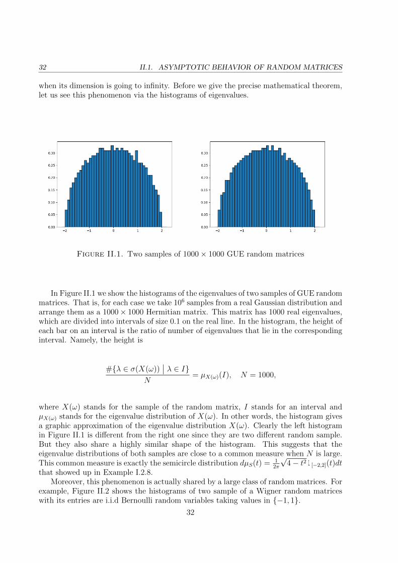
32 II.1. ASYMPTOTIC BEHAVIOR OF RANDOM MATRICES
when its dimension is going to infinity. Before we give the precise mathematical theorem,let us see this phenomenon via the histograms of eigenvalues.
Figure II.1. Two samples of 1000× 1000 GUE random matrices
In Figure II.1 we show the histograms of the eigenvalues of two samples of GUE randommatrices. That is, for each case we take 106 samples from a real Gaussian distribution andarrange them as a 1000× 1000 Hermitian matrix. This matrix has 1000 real eigenvalues,which are divided into intervals of size 0.1 on the real line. In the histogram, the height ofeach bar on an interval is the ratio of number of eigenvalues that lie in the correspondinginterval. Namely, the height is
#λ ∈ σ(X(ω))∣∣ λ ∈ I
N= µX(ω)(I), N = 1000,
where X(ω) stands for the sample of the random matrix, I stands for an interval andµX(ω) stands for the eigenvalue distribution of X(ω). In other words, the histogram givesa graphic approximation of the eigenvalue distribution X(ω). Clearly the left histogramin Figure II.1 is different from the right one since they are two different random sample.But they also share a highly similar shape of the histogram. This suggests that theeigenvalue distributions of both samples are close to a common measure when N is large.This common measure is exactly the semicircle distribution dµS(t) = 1
2π
√4− t21[−2,2](t)dt
that showed up in Example I.2.8.Moreover, this phenomenon is actually shared by a large class of random matrices. For
example, Figure II.2 shows the histograms of two sample of a Wigner random matriceswith its entries are i.i.d Bernoulli random variables taking values in −1, 1.
32
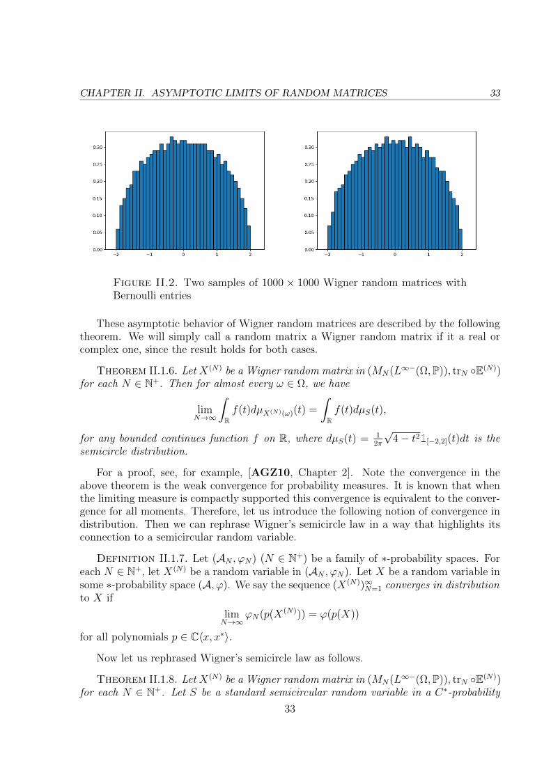
CHAPTER II. ASYMPTOTIC LIMITS OF RANDOM MATRICES 33
Figure II.2. Two samples of 1000 × 1000 Wigner random matrices withBernoulli entries
These asymptotic behavior of Wigner random matrices are described by the followingtheorem. We will simply call a random matrix a Wigner random matrix if it a real orcomplex one, since the result holds for both cases.
Theorem II.1.6. Let X(N) be a Wigner random matrix in (MN(L∞−(Ω,P)), trN E(N))for each N ∈ N+. Then for almost every ω ∈ Ω, we have
limN→∞
∫Rf(t)dµX(N)(ω)(t) =
∫Rf(t)dµS(t),
for any bounded continues function f on R, where dµS(t) = 12π
√4− t21[−2,2](t)dt is the
semicircle distribution.
For a proof, see, for example, [AGZ10, Chapter 2]. Note the convergence in theabove theorem is the weak convergence for probability measures. It is known that whenthe limiting measure is compactly supported this convergence is equivalent to the conver-gence for all moments. Therefore, let us introduce the following notion of convergence indistribution. Then we can rephrase Wigner’s semicircle law in a way that highlights itsconnection to a semicircular random variable.
Definition II.1.7. Let (AN , ϕN) (N ∈ N+) be a family of ∗-probability spaces. Foreach N ∈ N+, let X(N) be a random variable in (AN , ϕN). Let X be a random variable insome ∗-probability space (A, ϕ). We say the sequence (X(N))∞N=1 converges in distributionto X if
limN→∞
ϕN(p(X(N))) = ϕ(p(X))
for all polynomials p ∈ C〈x, x∗〉.
Now let us rephrased Wigner’s semicircle law as follows.
Theorem II.1.8. Let X(N) be a Wigner random matrix in (MN(L∞−(Ω,P)), trN E(N))for each N ∈ N+. Let S be a standard semicircular random variable in a C∗-probability
33

34 II.2. ASYMPTOTIC FREENESS AND STRONG ASYMPTOTIC FREENESS
space (A, ϕ). Then the sequence (X(N))∞N=1 almost surely converges in distribution to S,that is, for almost every ω ∈ Ω,
limN→∞
trN((X(N)(ω))k) = ϕ(Sk) for all k ∈ N+.
So far we have seen that a semicircular random variable can be regarded as a mode thatdescribes the limiting eigenvalue distribution of Wigner matrices as their dimension goesto infinity. This connection between Wigner matrices and semicircular random variablescan be also seen from other asymptotic phenomena. For example, we also know thatalmost surely
limN→∞
‖X(N)(ω)‖MN (C) = 2.
For a reference, see, for example, [BY88]. On the other hand, we also know that ‖S‖ = 2for a standard semicircular random variable S.
In Section II.2, more connections between Wigner random matrices and semicircularrandom variables will be presented. Of course, these connections between random matricesand non-commutative random variables hold actually for a large family of random matrixmodels and their corresponding limiting operators. In particular, let us mention thatHaar unitary random matrices almost surely converge in distribution to a Haar unitaryrandom variable when their dimension tends to infinity.
II.2. Asymptotic freeness and strong asymptotic freeness
In this section, we will strengthen the connection between random matrices and non-commutative random variables to the multi-variable case. In particular, we will see thatindependent copies of Wigner random matrices converge in distribution to freely indepen-dent semicircular random variables.
First, let us extend the convergence in distribution to the multi-variable case. Itnaturally leads us to the notion of asymptotic free independence.
Definition II.2.1. Let (AN , ϕN) (N ∈ N+) be a family of ∗-probability spaces. For
each N ∈ N+, let X(N) = (X(N)1 , . . . , X
(N)d ) be a d-tuple of random variables in (AN , ϕN).
Let X = (X1, . . . , Xd) denote a d-tuple of random variables in some ∗-probability space(A, ϕ).
(i) We say the sequence (X(N))∞N=1 converges in distribution to X if
limN→∞
ϕN(p(X(N))) = ϕ(p(X))
for any polynomial p ∈ C〈x1, . . . , xd, x∗1 . . . , x
∗d〉.
(ii) Suppose that the sequence (X(N))∞N=1 converges in distribution to X. If X is atuple of freely independent random variables in (A, ϕ), then we say (X(N))∞N=1
is asymptotically freely independent .
Asymptotic free independence for random matrices is one of the fundamental discover-ies of Voiculescu. This discovery tells us that Wigner’s semicircle law for Wigner randommatrices is not a mere coincidence. It reveals a deep link between free probability theoryand random matrix theory.
34
CHAPTER II. ASYMPTOTIC LIMITS OF RANDOM MATRICES 35
Now let us state the asymptotic freeness for Gaussian Wigner random matrices. We
say random matrices X(N)1 , . . . , X
(N)d are independent if their entries (divided into real
and imaginary parts for the complex case) form a set of independent random variables.
Theorem II.2.2. (See [Voi91]) Let X(N) = (X(N)1 , . . . , X
(N)d ) be a tuple of independent
Gaussian Wigner random matrices in (MN(L∞−(Ω,P)), trN E(N)) for each N ∈ N+.Then the sequence (X(N))∞N=1 converges in distribution to a tuple S = (S1, . . . , Sd) offreely independent semicircular random variables in some C∗-probability space, that is,
limN→∞
E[trN(p(X(N)(ω)))] = ϕ(p(S)),
for every p ∈ C〈x1, . . . , xd〉.
The theorem indeed can be strengthened to the almost surely convergence in distri-bution; see [HP00a, Tho00] and [MS17, Remark 5.14]. Moreover, the assumption thatthe entries of our random matrices are Gaussian can be weakened; see [Dyk93] for thealmost surely convergence of independent Wigner random matrices.
For independent Haar unitary random matrices, naturally we would expect that theyalmost surely converge in distribution to freely independent Haar unitary random vari-ables. We refer to [HP00a] for a proof of this theorem.
Theorem II.2.3. Let U (N) = (U(N)1 , . . . , U
(N)d ) be a tuple of independent Haar unitary
random matrices in (MN(L∞−(Ω,P)), trN E(N)) for each N ∈ N+. Then the sequence(U (N))∞N=1 almost surely converges in distribution to a tuple U = (U1, . . . , Ud) of freelyindependent Haar unitary random variables in some C∗-probability space, that is, foralmost every ω ∈ Ω
limN→∞
trN(p(U (N)(ω))) = ϕ(p(U)),
for every p ∈ C〈x1, . . . , xd, x∗1, . . . , x
∗d〉.
Recall that we have mentioned at the end of Section II.1 that we have almost surely
limN→∞
‖X(N)(ω)‖MN (C) = ‖S‖
for Wigner random matrices X(N) and a semicircular random variable S. Such a result canalso be strengthened to the multi-variable case and also to other random matrix models.Let us first introduce the notion of strong convergence in distribution to describe thisphenomenon.
Definition II.2.4. Let X(N) = (X(N)1 , . . . , X
(N)d ) be a tuple of random matrices in
(MN(L∞−(Ω,P)), trN E(N)) for eachN ∈ N+. LetX = (X1, . . . , Xd) be a tuple of randomvariables in a C∗-probability space (A, ϕ). We say the sequence (X(N))∞N=1 almost surelystrongly converges in distribution to X if
(i) (X(N))∞N=1 almost surely converges in distribution to X, i.e. for almost everyω ∈ Ω.
limN→∞
trN(p(X(N)(ω))) = ϕ(p(X))
for every p ∈ C〈x1, . . . , xd, x∗1, . . . , x
∗d〉.
35

36 II.2. ASYMPTOTIC FREENESS AND STRONG ASYMPTOTIC FREENESS
(ii) we also have for almost every ω ∈ Ω
limN→∞
‖p(X(N)(ω))‖MN (C) = ‖p(X)‖A
for every p ∈ C〈x1, . . . , xd, x∗1, . . . , x
∗d〉.
For succinctness, we will abuse the notation and write the norms ‖ · ‖MN (C) and ‖ · ‖Aas ‖ · ‖ in the following.
Theorem II.2.5. (See [HT05, HST06]) Let X(N) = (X(N)1 , . . . , X
(N)d ) be a tuple
of independent GUE random matrices in (MN(L∞−(Ω,P)), trN E(N)) for each N ∈ N+.Then the sequence (X(N))∞N=1 almost surely strongly converges in distribution to a tu-ple S = (S1, . . . , Sd) of freely independent semicircular random variables in some C∗-probability space.
For GOE and GSE (Gaussian symplectic ensemble) random matrices, their strongconvergence in distribution toward freely independent semicircular random variables wasproven in [Sch05]. For the Wigner case, this result was proven in [CD07, And13]. AHaar unitary version of this theorem also holds, see [CM14].
In Chapter VII, we will see that these connections between random matrices and non-commutative random variables can be further strengthened. But our strengthening goesin a different way than the results above. In Definition II.2.1 and II.2.4, we note that theconvergence is always stated for non-commutative polynomials. In Chapter VII, we willsee that polynomials can be extended to a larger class of non-commutative functions thatinvolve the inverse of variables.
36
CHAPTER III
Inner rank
In this chapter we focus on a purely algebraic concept—the inner rank—and somerelated algebraic concepts, for example, central eigenvalues. The analytic counterpart ofthe inner rank over polynomials was introduced in Definition I.5.10 as an analytic rankover von Neumann algebras. An equality will be established in Section V.2 between thisanalytic rank and the inner rank over polynomials. Moreover, we will also correspond thecentral eigenvalues with their analytic counterparts in Section VI.2. These counterpartswere described in Section I.3 under the name of zero divisors or atoms.
The inner rank is a generalization of the usual notion of rank in linear algebra where thecomplex numbers are replaced by more general rings. In Section III.1, we will introducethe inner rank for matrices over a unital (not necessarily commutative) complex algebra.Then we will pay special attention to the case when the algebra is stably finite or a divisionring.
In Section III.2, we will limit our discussion of the inner rank to the case of Sylvesterdomains. Sylvester domains are of particular interest for us because they characterize ringsthat can be embedded into division rings with inner rank preserving homomorphisms (seeTheorem IV.2.5 in the next chapter). The embeddability of non-commutative polynomialsinto a division ring with the inner rank preserved is a crucial property which will be usedin Section V.2. So the algebras of polynomials give us the practical example amongSylvester domains. After that we will focus on the case of polynomials until the end ofthis chapter.
In Section III.3, some zero block structure of linear matrices over non-commutativepolynomials will be presented. Such a structure will allow us later to do an inductiveargument on the dimension of matrices in the proof of Theorem V.1.1.
Section III.4 is a brief introduction to central eigenvalues. It is well-known that eigen-values can be defined by the invertibility of matrices (which is equivalent to the fullness ofthe usual rank). Here we replace the invertibility by the maximality of the inner rank todefine these central eigenvalues. It is a natural concept if we treat the inner rank as a gen-eralization of the usual rank. Two facts on central eigenvalues will be given: one about thecardinality of central eigenvalues of a given matrix and one about the possible positionsof central eigenvalues when the given matrix is linear. These two facts can be used to pre-dict the cardinality and positions of atoms for distributions of some matrix-valued randomvariables, since we have the aforementioned correspondence between central eigenvaluesand atoms.
III.1. Some basics of the inner rank
LetA be a general unital (not necessarily commutative) complex algebra. By Mm,n(A)we denote the m× n matrices with entries in A; and we set Mn(A) := Mn,n(A).
37
38 III.1. SOME BASICS OF THE INNER RANK
Definition III.1.1. For any non-zero A ∈ Mm,n(A), the inner rank of A is definedas the least positive integer r such that there are matrices P ∈ Mm,r(A), Q ∈ Mr,n(A)satisfying A = PQ. We denote this number by ρ(A), and we call any such factorizationwith r = ρ(A) a rank factorization. Additionally, if A is a zero matrix, we define ρ(A) = 0.
For example, it is easy to verify the factorization(y2 yxyyxy yx2y
)=
(yyx
)(y xy
)in matrices over C〈x, y〉. So, this matrix has inner rank 1: its inner rank has to be lessthan or equal to 1 by the above factorization and it is not a zero matrix. Moreover, anyelement in A, regarded as a 1× 1 matrix, has inner rank 1 unless it is 0.
This notion of inner rank was defined in [Ber67], but goes back much further accordingto a commment in [Coh06, Chapter 0]: “almost any pre-1914 book on matrix theorydefines the rank of a matrix A as the least number of terms in the expression of A as asum of dyads , i.e. products of a column by a row, which is a matrix of inner rank 1”.
It is clear that the inner rank of an m× n matrix is less than or equal to minm,n.Those matrices maximizing their inner ranks play a very important role and thus we havethe following definition for them.
Definition III.1.2. A non-zero matrixA ∈Mm,n(A) is called full if ρ(A) = minm,n,namely, if there is no rank factorization with ρ(A) < minm,n.
When we set A to be a unital complex algebra, Mn(C) always becomes a subalgebraof Mn(A) for any n ∈ N+. Moreover, it is not difficult to check that the inner rankagrees with the usual notion of rank for matrices over C, so the inner rank generalizesconsistently the notion of rank from Mn(C) to Mn(A).
In the following remarks, we record some basic properties for the inner rank to depictmore analogies between the inner rank and the usual rank. These properties follow directlyby the definition of inner rank.
Remark III.1.3. Let A ∈Mm,n(A) be given.
(i) For any invertible B ∈Mm(A) and C ∈Mn(A), we have
ρ(A) = ρ(BAC).
(ii) For any B ∈Mn,s(A), we have
ρ(AB) ≤ minρ(A), ρ(B).(iii) If we write A = (B C), where B is the block of the first r columns of A and C
consists of the remaining columns, then
ρ(A) ≥ maxρ(B), ρ(C).Additionally, if C = 0, then ρ(A) = ρ(B). Moreover, similar inequality alsoholds if we partition A by rows.
(iv) For any B ∈Mp,q(A), the diagonal sum of A and B, i.e.,
A⊕B :=
(A 00 B
)∈Mm+p,n+q(A)
38
CHAPTER III. INNER RANK 39
satisfies ρ(A⊕B) ≤ ρ(A) + ρ(B). Combining this inequality with Item (iii), wehave in particular
maxρ(A), ρ(B) ≤ ρ(A⊕B) ≤ ρ(A) + ρ(B).
(v) For any ring homomorphism ϕ defined on A,
ρ(ϕ(A)) ≤ ρ(A),
where ϕ(A) stands for the entrywise image of A under ϕ.
According to the definition, the inner rank measures some “non-degenerateness” ofmatrices via their factorizations. So one may be tempted to believe that full square ma-trices are invertible or vice versa. However, neither is true without any further assumptionon the algebra A. For example, any non-zero element is a full 1×1 matrix but may not beinvertible in general. To see that an invertible matrix might not be full, one can considerthe following example.
Example III.1.4. For any integers m and n satisfying 1 ≤ m < n, let A be the unitalalgebra A generated by 2mn generators, arranged as an n ×m matrix A and an m × nmatrix B, and by the defining relations AB = 1n. Clearly the identity matrix 1n is notfull by the defining relations of A while it is always invertible.
Fortunately, we will not encounter such algebras over which the inner rank behavesbadly. Instead we always consider algebras with the following property.
Definition III.1.5. A unital algebra A is called stably finite (or weakly finite) if forall n ∈ N+ and all A,B ∈Mn(A), AB = 1n implies BA = 1n.
Over a stably finite algebra we have that every invertible matrix is full. Actually, wehave a more general result as follows.
Proposition III.1.6. ([Coh06, Proposition 5.4.6]) Suppose that A is stably finite.Let A ∈Mm+n(A) be of the form
A =
(B CD E
),
where B ∈ Mm(A), C ∈ Mm,n(A), D ∈ Mn,m(A) and E ∈ Mn(A). If B is invertible,then ρ(A) ≥ m, with equality if and only if E = DB−1C.
Now if we assume that all full matrices are invertible over an algebra A, then inparticular all non-zero elements are invertible in A. That is, A has to be a division ringor skew field . Actually, this condition is not only necessary, but also sufficient. We recordthis fact here by the following lemma.
Lemma III.1.7. If A is a division ring, then every full square matrix over A is invert-ible.
Proof. It is clear that the result holds for matrices of dimension 1. We proceed bymathematical induction on the dimension of matrices. Suppose that the result holds formatrices of dimension n and A is a full matrix in Mn+1(A). On the one hand, A is non-zero, so at least one entry of A is non-zero. On the other hand, permutations of rows and
39
40 III.1. SOME BASICS OF THE INNER RANK
columns preserve the fullness of A. Thus we can assume the (1, 1)-entry of A is non-zero.That is, we can assume that A has the form
A =
(a bc D
)with a 6= 0. With the invertible matrices
U :=
(1 0
−ca−1 1n
), V :=
(a−1 −a−1b0 1n
)∈Mn+1(A),
we obtain another full matrix
UAV =
(1 00 D − ca−1b
),
where the block D−ca−1b has to be a full matrix by Item (iv) of Remark III.1.3. Therefore,by induction hypothesis we see that D − ca−1b is invertible. It follows that UAV isinvertible and thus A is also invertible.
Actually, we see that a non-commutative version of the Gaussian elimination methodworks equally well over a division ring (which may not be commutative in general), fromthe proof of the above lemma. The matrices U and V in the above proof play a role ofrow and column operations. Moreover, we will obtain a diagonal matrix from which theinner rank of the original matrix can be directly read off if we continue this algorithm toits end. We record this fact here as the following proposition.
Proposition III.1.8. Suppose that A is a division ring. Then for any matrix A overA, there exist two invertible matrices U and V over A such that
UAV =
(1ρ(A) 0
0 0
).
Proof. If A 6= 0, then we implement the non-commutative Gaussian eliminationmethod to A. That means there are invertible matrices U and V such that
UAV =
(1r 00 0
)for some r ∈ N+. So it remains to show that ρ(A) = r, or equivalently,
ρ(UAV ) = ρ
(1r 00 0
)= r.
If we recall the inequality in Item (iv) of Remark III.1.3, we see that ρ(UAV ) = ρ(1r).Therefore, we only need to show ρ(1r) = r, i.e., 1r is full. As an invertible matrix, 1r isindeed full if A is stably finite. Hence the proof is completed by the well-known fact thata division algebra is stably finite.
40
CHAPTER III. INNER RANK 41
III.2. Sylvester domains
Our main goal of this section is to present some properties of the algebra C〈x1, . . . , xd〉of non-commutative polynomials. At this point, we want to introduce these properties atring theoretic level to highlight them. At the end of this section, we will come back tothe algebra C〈x1, . . . , xd〉.
These properties are actually shared by more general rings known as Sylvester do-mains. So we will first introduce Sylvester domains as well as some basic properties ofthem. Then we will give the reason why C〈x1, . . . , xd〉 is a Sylvester domain.
Moreover, a difference appears here between the commutative and the non-commutativepolynomials. That is, the algebra C[x1, . . . , xd] of commutative polynomials with d > 2 isnot a Sylvester domain, which has some consequence during our investigations in SectionV.2.
Definition III.2.1. ([DS78]) A non-zero ring A is called a Sylvester domain if forany A ∈Mm,n(A), B ∈Mn,r(A) such that AB = 0, it follows that
ρ(A) + ρ(B) ≤ n.
In particular, if two elements a and b satisfy ab = 0, then ρ(a) + ρ(b) ≤ 1 according tothe definition of Sylvester domain. This implies that a = 0 or b = 0. So Sylvester domainsare indeed domains. The reason for naming these domains after Sylvester is that they areactually equivalently characterized by Sylvester’s law of nullity or rank inequality withrespect to the inner rank, that is, for any A ∈Mm,n(A), B ∈Mn,r(A),
ρ(A) + ρ(B) ≤ ρ(AB) + n.
Apparently the defining property in Definition III.2.1 is a weaker form of Sylvester’s lawof nullity. A proof for that it implies the law of nullity can be found in [DS78] or [Coh06,Section 5.5].
Clearly, (commutative) fields satisfy Sylvester’s law of nullity due to Sylvester, andtherefore they are Sylvester domains. More generally, division rings are also Sylvesterdomains. To see this, let A and B be two matrices over a division ring A satisfyingAB = 0. By Proposition III.1.8 we can find invertible matrices U and V such that
UAV =
(1ρ(A) 0
0 0
).
By writing
V −1B =
(B1 B2
B3 B4
),
where B1 ∈Mρ(A)(A) and other blocks are of appropriate size, we have(1ρ(A) 0
0 0
)(B1 B2
B3 B4
)= (UAV )(V −1B) = UAB = 0.
This enforces that B1 = B2 = 0, which implies that
ρ(V −1B) = ρ
(0 0B3 B4
)= ρ
(B3 B4
)41

42 III.2. SYLVESTER DOMAINS
according to Item (iii) of Remark III.1.3. Note (B3 B4) is an (n− ρ(A))× n matrix, weconclude that
ρ(V −1B) ≤ n− ρ(A).
Hence ρ(B) ≤ n− ρ(A) follows.An immediate consequence of Sylvester’s law of nullity is that the product of full
square matrices is again full over a Sylvester domain. However, this may not be true ingeneral. Instead we only have an upper bound for the inner rank of a product of fullmatrices by Item (ii) of Remark III.1.3.
Moreover, for any matrices A and B the inequality ρ(A⊕ B) ≤ ρ(A) + ρ(B) in Item(iv) of Remark III.1.3 becomes an equality for the case of A = C, which is well-knownin linear algebra. However, this equality also fails in general. For example, if we choosem = 1 and n = 2 for the algebra in Example III.1.4, then 12 is the diagonal sum oftwo copies of 1 but has inner rank 1. However, this equality indeed holds for Sylvesterdomains, which we record as the following lemma.
Lemma III.2.2. (See [DS78] or [Coh06, Lemma 5.5.3]) Let A be a Sylvester domain.Then for any matrices A, B over A,
ρ(A⊕B) = ρ(A) + ρ(B).
A well-known characterization of the usual rank of a scalar-valued matrix is givenby submatrices. Now we can state its analogue for the inner rank over Sylvester do-mains. That is, the inner rank of a matrix is given by the maximal dimension of itsfull submatrices. This characterization was first proven by Cohn for a special class ofSylvester domains called semifir in [Coh74]. But it actually holds under weaker assump-tions. These assumptions are exactly the two properties of Sylvester domain as explainedabove.
Theorem III.2.3. (See [DS78] or [Coh06, Theorem 5.4.9]) Suppose that the set ofall full square matrices over A is closed under products and diagonal sums. Then forany A ∈ Mm,n(A), there exists a square submatrix of A which is a full matrix over A ofdimension ρ(A). Moreover, ρ(A) is the maximal dimension for such submatrices.
The most important example of Sylvester domains for us is the algebra C〈x1, . . . , xd〉of non-commutative polynomials. However, it is far from obvious that C〈x1, . . . , xd〉 isa Sylvester domain. Briefly, the reason is that C〈x1, . . . , xd〉 has the following property:For any matrices A, B over C〈x1, . . . , xd〉 satisfying AB = 0, there exists an invertiblesquare matrix U over C〈x1, . . . , xd〉 such that
AU =(C 0
), U−1B =
(0D
),
where the number of C’s columns is the same as the number of rows of the zero block inU−1B. Then it is easy to see that ρ(A)+ρ(B) = ρ(AU) + ρ(BU−1) ≤ n, where n denotesthe number of columns of A.
A matrix relation expressed as AB = 0 is called trivial if for each i = 1, . . . , n eitherthe i-th column of A or the i-th row of B is 0. So the property in the above paragraphsays that every matrix relation AB = 0 for two matrices A and B can be trivialized byinvertible matrices over C〈x1, . . . , xd〉. For example, A = (x, xy) and B = (yz,−z)T gives
42

CHAPTER III. INNER RANK 43
a relation AB = 0 which is not trivial over C〈x, y, z〉, but it can be trivialized by aninvertible matrix
U =
(1 y0 −1
)because AU = (x, 0) and U−1B = (0, z)T .
Moreover, this property, the trivialization for any matrix relation AB = 0, is sharedby a general class of Sylvester domains, namely, semifirs. Semifirs have been mentionedbefore Theorem III.2.3 without definition. Again we will not go further into the details ofsemifirs here. Instead we refer the interested reader to [Coh06, Section 2.3] for its precisedefinition. But we want to point out here that this trivialization property is actually oneof the many equivalent characterizations of semifirs.
Then it remains to check that C〈x1, . . . , xd〉 is a semifir in order to see it is a Sylvesterdomain. This is still not an easy task but it turns out to be sufficient to check the matrixrelation AB = 0 for the special case that A is a row vector and B a column vector(see [Coh06, Section 2.3] for the details). So let us take a closer look at an n-termrelation
∑ni=1 piqi = 0, where pi, qi ∈ C〈x1, . . . , xd〉, i = 1 . . . , n. This particular relation
says that (p1, . . . , pn) is right linear dependent over C〈x1, . . . , xd〉. So if we can find aninvertible matrix which reduces (p1, . . . , pn), by acting on the right, to a tuple whose non-zero entries are right linear independent over C〈x1, . . . , xd〉, then the relation is trivializedby this invertible matrix. This reduction is indeed feasible by an algorithm. However,describing such an algorithm requires some extra effort and deviates a lot from our originalquest here. So we leave out the details here and refer the interested reader to [Coh06,Theorem 2.5.1]. Actually, in [Coh06, Section 2.4], a notion called weak algorithm wasdeveloped (as a generalization of the division algorithm) to do this job. Any ring withweak algorithm was also proven to be a semifir; see [Coh06, Theorem 2.4.4]. At lastbut not least, [Coh06, Corollary 2.5.2] and the paragraph thereafter tell us that the freealgebra C〈x1, . . . , xd〉 indeed satisfies the weak algorithm.
Therefore, we are finally able to record:
Example III.2.4. The algebra C〈x1, . . . , xd〉 of non-commutative polynomials in dvariables is a Sylvester domain for any d ∈ N+. Hence, by Theorem III.2.3, the inner rankof a matrix over C〈x1, . . . , xd〉 is given by the maximal dimension of its submatrices.
So far we have seen that Sylvester domains are domains on which the inner rankbehaves very nicely. Furthermore, they include important examples such as algebras ofnon-commutative polynomials. However, they do not include commutative polynomialsif there are more than two variables. We record this fact by the following remark.
Remark III.2.5. The algebra C[x1, . . . , xd] of commutative polynomials is a Sylvesterdomain if and only if d = 1 or d = 2.
The fact that C[x1, . . . , xd] is a Sylvester domain when d = 1, 2 can be extracted from[Coh06, Theorem 5.5.4]. To see that the other cases are not Sylvester domains, it isenough to find two matrices over C[x, y, z] that fail the defining property. The followingexample, taken from [Coh06, Section 5.5], provides us an example that fails the defining
43

44 III.3. LINEAR MATRICES
property. Let us consider
A =
0 z −y−z 0 xy −x 0
, B =
xyz
.
Then it is clear that AB = 0 and ρ(B) = 1. Moreover, it can be proven that A is full, i.e.,ρ(A) = 3. Therefore, ρ(A) + ρ(B) = 4 > 3, which tells us that C[x, y, z] is not a Sylvesterdomain.
The purpose of introducing Sylvester domains in [DS78] was to study rings that canbe embedded into division rings by inner rank-preserving homomorphisms. This propertywas first proven for semifirs by Cohn. It turned out to be exactly an equivalent descrip-tion of Sylvester domain; see Theorem IV.2.5 for the precise statement. Therefore, as aSylvester domain, C〈x1, . . . , xd〉 can be embedded into some division ring. Let us recallthat commutative polynomials can be embedded into the field of rational functions. Withthat in mind, it is not surprising that the division ring of non-commutative rational func-tions also exists and thus extends C〈x1, . . . , xd〉. But we postpone the related discussionto the next chapter since these non-commutative rational functions are very importantfor our investigation in Section V.2 and deserve a whole chapter.
III.3. Linear matrices
From now on, we will focus on the algebra C〈x1, . . . , xd〉 of non-commutative polynomi-als. This short section is devoted to special matrices whose entries are linear polynomials,i.e., polynomials of degree at most 1. These matrices have some zero block structure asmentioned in the introduction of this chapter. Our goal of this section is to present thisstructure in details.
In order to introduce this structure, let us first consider a matrix of the form
A =
(B 0C D
)∈Mn(C〈x1, . . . , xd〉),
which has a zero block of size r×s and blocks B, C, D of sizes r×(n−s), (n−r)×(n−s),(n− r)× s, respectively. Then we have the factorization
A =
(B 0C D
)=
(B 00 1n−r
)(1n−s 0C D
).
So A has been expressed as a product of an n× (2n−r−s) matrix and an (2n−r−s)×nmatrix. This allows us to conclude that ρ(A) ≤ 2n − r − s. Therefore, if the size of thezero block of A satisfies r + s > n, we have ρ(A) < n, which means that A is not full.Such matrices are called hollow matrices.
Definition III.3.1. A matrix in Mn(C〈x1, . . . , xd〉) is called hollow if it has an r × sblock of zeros with r + s > n.
In general, a non-full A ∈Mn(C〈x1, . . . , xd〉) may not have any zero blocks or subma-trices. However, we can say more for the following special matrices.
44
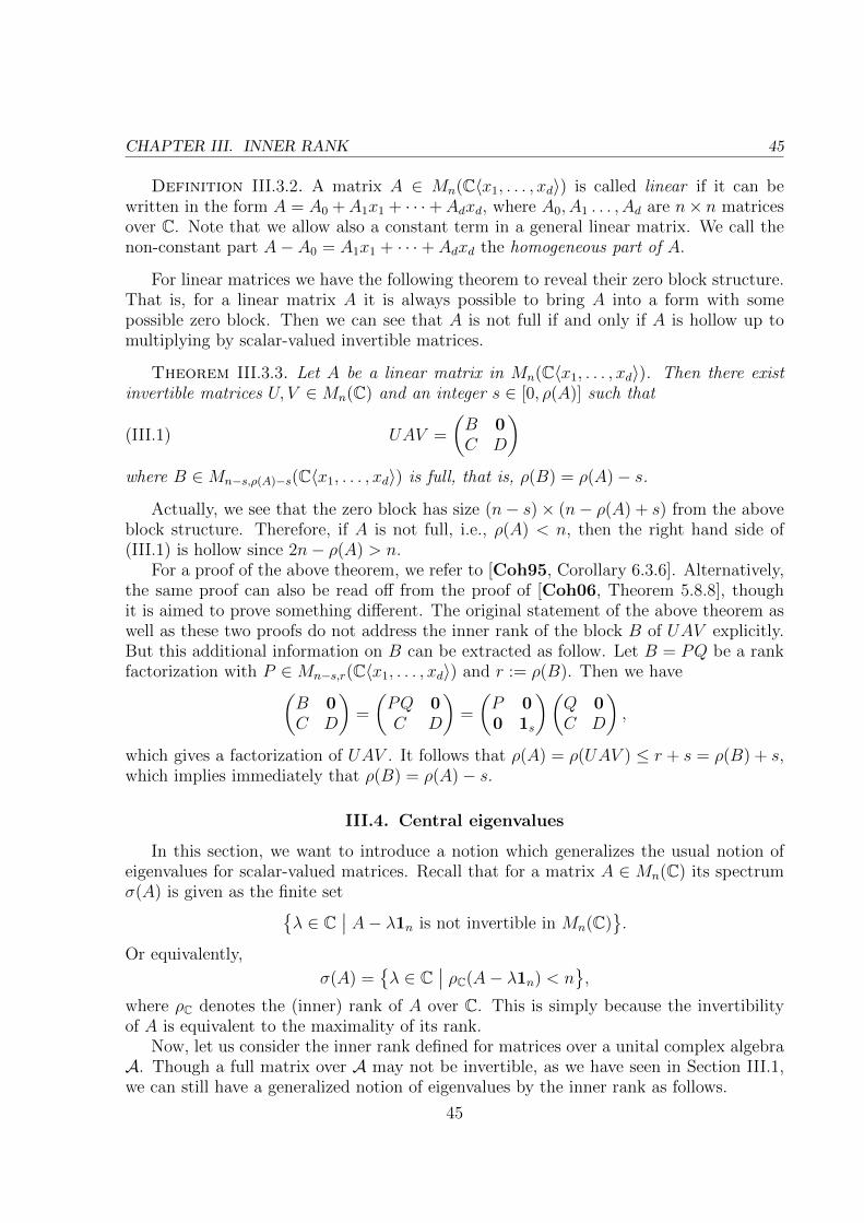
CHAPTER III. INNER RANK 45
Definition III.3.2. A matrix A ∈ Mn(C〈x1, . . . , xd〉) is called linear if it can bewritten in the form A = A0 +A1x1 + · · ·+Adxd, where A0, A1 . . . , Ad are n× n matricesover C. Note that we allow also a constant term in a general linear matrix. We call thenon-constant part A− A0 = A1x1 + · · ·+ Adxd the homogeneous part of A.
For linear matrices we have the following theorem to reveal their zero block structure.That is, for a linear matrix A it is always possible to bring A into a form with somepossible zero block. Then we can see that A is not full if and only if A is hollow up tomultiplying by scalar-valued invertible matrices.
Theorem III.3.3. Let A be a linear matrix in Mn(C〈x1, . . . , xd〉). Then there existinvertible matrices U, V ∈Mn(C) and an integer s ∈ [0, ρ(A)] such that
(III.1) UAV =
(B 0C D
)where B ∈Mn−s,ρ(A)−s(C〈x1, . . . , xd〉) is full, that is, ρ(B) = ρ(A)− s.
Actually, we see that the zero block has size (n− s)× (n− ρ(A) + s) from the aboveblock structure. Therefore, if A is not full, i.e., ρ(A) < n, then the right hand side of(III.1) is hollow since 2n− ρ(A) > n.
For a proof of the above theorem, we refer to [Coh95, Corollary 6.3.6]. Alternatively,the same proof can also be read off from the proof of [Coh06, Theorem 5.8.8], thoughit is aimed to prove something different. The original statement of the above theorem aswell as these two proofs do not address the inner rank of the block B of UAV explicitly.But this additional information on B can be extracted as follow. Let B = PQ be a rankfactorization with P ∈Mn−s,r(C〈x1, . . . , xd〉) and r := ρ(B). Then we have(
B 0C D
)=
(PQ 0C D
)=
(P 00 1s
)(Q 0C D
),
which gives a factorization of UAV . It follows that ρ(A) = ρ(UAV ) ≤ r + s = ρ(B) + s,which implies immediately that ρ(B) = ρ(A)− s.
III.4. Central eigenvalues
In this section, we want to introduce a notion which generalizes the usual notion ofeigenvalues for scalar-valued matrices. Recall that for a matrix A ∈ Mn(C) its spectrumσ(A) is given as the finite set
λ ∈ C∣∣ A− λ1n is not invertible in Mn(C)
.
Or equivalently,
σ(A) =λ ∈ C
∣∣ ρC(A− λ1n) < n,
where ρC denotes the (inner) rank of A over C. This is simply because the invertibilityof A is equivalent to the maximality of its rank.
Now, let us consider the inner rank defined for matrices over a unital complex algebraA. Though a full matrix over A may not be invertible, as we have seen in Section III.1,we can still have a generalized notion of eigenvalues by the inner rank as follows.
45
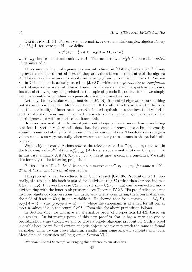
46 III.4. CENTRAL EIGENVALUES
Definition III.4.1. For every square matrix A over a unital complex algebra A, sayA ∈Mn(A) for some n ∈ N+, we define
σfullA (A) :=
λ ∈ C
∣∣ ρA(A− λ1n) < n,
where ρA denotes the inner rank over A. The numbers λ ∈ σfullA (A) are called central
eigenvalues of A.
This concept of central eigenvalues was introduced in [Coh85, Section 8.4].1 Theseeigenvalues are called central because they are values taken in the centre of the algebraA. The centre of A is, in our special case, exactly given by complex numbers C. Section8.4 in Cohn’s book is actually based on [Jac37], which is on pseudo-linear transforms .Central eigenvalues were introduced therein from a very different perspective than ours.Instead of studying anything related to the topic of pseudo-linear transforms, we simplyintroduce central eigenvalues as a generalization of eigenvalues here.
Actually, for any scalar-valued matrix in Mn(A), its central eigenvalues are nothingbut its usual eigenvalues. Moreover, Lemma III.1.7 also teaches us that the fullness,i.e., the maximality of inner rank over A is indeed equivalent to the invertibility if A isadditionally a division ring. So central eigenvalues are reasonable generalization of theusual eigenvalues with respect to the inner rank.
However, our motivation to investigate central eigenvalues is more than generalizinga notion. In Section VI.2, we will show that these central eigenvalues can become exactlyatoms of some probability distributions under certain conditions. Therefore, central eigen-values come to us very naturally when we want to study these atoms in the probabilisticcontext.
We specify our considerations now to the relevant case A = C〈x1, . . . , xd〉 and will inthe following write σfull(A) for σfull
C〈x1,...,xd〉(A) for any square matrix A over C〈x1, . . . , xd〉.In this case, a matrix A ∈Mn(C〈x1, . . . , xd〉) has at most n central eigenvalues. We statethis formally as the following proposition.
Proposition III.4.2. Let A be an n× n matrix over C〈x1, . . . , xd〉 for some n ∈ N+.Then A has at most n central eigenvalues.
This proposition can be deduced from Cohn’s result [Coh85, Proposition 8.4.1]. Ac-tually, the result in his book is stated for a division ring K rather than our specific caseC〈x1, . . . , xd〉. It covers the case C〈x1, . . . , xd〉 since C〈x1, . . . , xd〉 can be embedded into adivision ring with the inner rank preserved; see Theorem IV.2.5. His proof relied on someinvolved algebraic considerations, which is, very briefly, considering the given matrix overthe field of fraction K(t) in one variable t. He showed that for a matrix A ∈ Mn(K),ρK(t)(A − t) = supα∈C ρK(t)(A − α) = n, where the supremum is attained for all but atmost n values of α in the centre C of K. From this the above proposition follows.
In Section VI.2, we will give an alternative proof of Proposition III.4.2, based onour results. An interesting point of this new proof is that it has a very analytic orprobabilistic nature though we aim to prove a purely algebraic proposition. Such a proofis doable because we found certain analytic objects behave very much the same as formalvariables. Thus we can prove algebraic results using some analytic concepts and tools.More detailed discussion will be given in Section VI.2.
1We thank Konrad Schrempf for bringing this reference to our attention.
46

CHAPTER III. INNER RANK 47
Conversely, algebraic results like [Coh85, Proposition 8.4.1] will give us informationabout the corresponding analytic objects. So here we give another algebraic result oncentral eigenvalues. Unfortunately, for the following proposition, we do not know atmoment if there is an analytic or probabilistic proof or explanation.
Proposition III.4.3. Let any linear A ∈ Mn(C〈x1, . . . , xd〉) of the form A = A0 +A1x1 + · · · + Adxd with A0, A1, . . . , Ad ∈ Mn(C) be given. Then the following statementshold:
(i) We have that σfull(A) ⊂ σ(A0), where σ(A0) is the usual spectrum of A0 con-sisting of all eigenvalues of A0.
(ii) If the homogeneous part A− A0 of A is full, then σfull(A) = ∅.
Proof. Let λ ∈ σfull(A) be given. This means that A− λ1n is not full. So TheoremIII.3.3 guarantees the existence of invertible matrices U, V ∈Mn(C) such that
U(A− λ1n)V = U(A0 − λ1n)V +d∑j=1
(UAjV )xj
is hollow. Due to linearity, this enforces both U(A0 − λ1n)V and∑d
j=1(UAjV )xj to be
hollow. Now, on the one hand, it follows that neither U(A0−λ1n)V nor A0−λ1n, thanksto the invertibility of U and V , can be invertible. Thus, we infer that λ ∈ σ(A0), which
shows the validity of (i). On the other hand, we see that neither∑d
j=1(UAjV )xj nor∑dj=1Ajxj, by the invertibility of U and V , can be full. Thus, if the homogeneous part of
A is assumed to be full, that contradiction rules out the existence of λ ∈ σfull(A), whichproves (ii).
47

CHAPTER IV
Free field
In this chapter, our first goal is to give an introduction to the free field, i.e., the univer-sal skew field of fractions of non-commutative polynomials. It is a follow-up introductionof Sylvester domains in the last chapter. Actually, universal skew field of fractions canbe constructed for any Sylvester domain with the inner rank preserved. This fundamen-tal result will be record as Theorem IV.2.5 (see [DS78] or [Coh06][Section 7.5]). Ourapplication of this result is going to the algebra C〈x1, . . . , xd〉. In this particular case,the resulting universal field of fractions, the free field, gives us the core objects—non-commutative rational functions—that will be investigated in the context of free proba-bility. Moreover, the free field provides us a much larger underlying algebra to considermatrices over polynomials. This will allow us to diagonalize a matrix of polynomials torecover its inner rank. This diagonalization idea will play an essential role for establish-ing the equality between the inner rank over polynomials and the analytic rank over vonNeumann algebra in Section V.2.
We will discuss universal skew fields of fractions in Section IV.2. Section IV.1 willbe devoted to an alternative approach to the free field. This approach provides us amore intuitive way to understand the free field, in comparison to the one in Section IV.2.Instead of building a skew field of fractions to extend C〈x1, . . . , xd〉, we will build rationalexpressions from C〈x1, . . . , xd〉 by arithmetic operations in this approach. When it comesto define the evaluation for rational expressions they are also much easier to define thanfor rational functions. The evaluation of rational functions will be discussed in SectionIV.4. At the end of Section IV.1, we will point out a link between rational expressionsand rational functions with the help of the evaluation of rational expressions.
An important concept related to rational functions, which will be given in SectionIV.3, is the linear representation. That is, each rational function can be associated withsome full matrix over linear polynomials. Similar concepts are known as the “linearizationtrick” in many different realms of mathematics. We will present an algorithm taken from[HMS18] to show how a linear representation can be build very explicitly for a rationalexpression.
In Section IV.4, we will handle the technical issue when we want to define the evalu-ation of rational functions. To achieve a reasonable definition of the evaluation, assump-tions like stable finiteness can not be avoided. We will give a self-contained proof for thewell-definedness of our definition of the evaluation.
Rational closure and division closure will be introduced Section IV.5. They will replacethe role of rational functions when we discuss the strong Atiyah property in Section V.3.Actually, the rational closure is given by all well-defined evaluations of rational functions.The division closure usually coincides with the rational closure in our consideration.
49
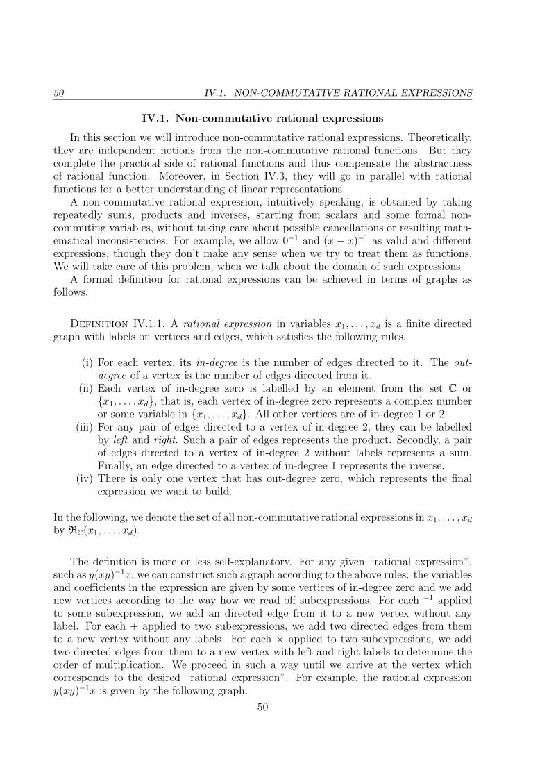
50 IV.1. NON-COMMUTATIVE RATIONAL EXPRESSIONS
IV.1. Non-commutative rational expressions
In this section we will introduce non-commutative rational expressions. Theoretically,they are independent notions from the non-commutative rational functions. But theycomplete the practical side of rational functions and thus compensate the abstractnessof rational function. Moreover, in Section IV.3, they will go in parallel with rationalfunctions for a better understanding of linear representations.
A non-commutative rational expression, intuitively speaking, is obtained by takingrepeatedly sums, products and inverses, starting from scalars and some formal non-commuting variables, without taking care about possible cancellations or resulting math-ematical inconsistencies. For example, we allow 0−1 and (x− x)−1 as valid and differentexpressions, though they don’t make any sense when we try to treat them as functions.We will take care of this problem, when we talk about the domain of such expressions.
A formal definition for rational expressions can be achieved in terms of graphs asfollows.
Definition IV.1.1. A rational expression in variables x1, . . . , xd is a finite directedgraph with labels on vertices and edges, which satisfies the following rules.
(i) For each vertex, its in-degree is the number of edges directed to it. The out-degree of a vertex is the number of edges directed from it.
(ii) Each vertex of in-degree zero is labelled by an element from the set C orx1, . . . , xd, that is, each vertex of in-degree zero represents a complex numberor some variable in x1, . . . , xd. All other vertices are of in-degree 1 or 2.
(iii) For any pair of edges directed to a vertex of in-degree 2, they can be labelledby left and right. Such a pair of edges represents the product. Secondly, a pairof edges directed to a vertex of in-degree 2 without labels represents a sum.Finally, an edge directed to a vertex of in-degree 1 represents the inverse.
(iv) There is only one vertex that has out-degree zero, which represents the finalexpression we want to build.
In the following, we denote the set of all non-commutative rational expressions in x1, . . . , xdby RC(x1, . . . , xd).
The definition is more or less self-explanatory. For any given “rational expression”,such as y(xy)−1x, we can construct such a graph according to the above rules: the variablesand coefficients in the expression are given by some vertices of in-degree zero and we addnew vertices according to the way how we read off subexpressions. For each −1 appliedto some subexpression, we add an directed edge from it to a new vertex without anylabel. For each + applied to two subexpressions, we add two directed edges from themto a new vertex without any labels. For each × applied to two subexpressions, we addtwo directed edges from them to a new vertex with left and right labels to determine theorder of multiplication. We proceed in such a way until we arrive at the vertex whichcorresponds to the desired “rational expression”. For example, the rational expressiony(xy)−1x is given by the following graph:
50
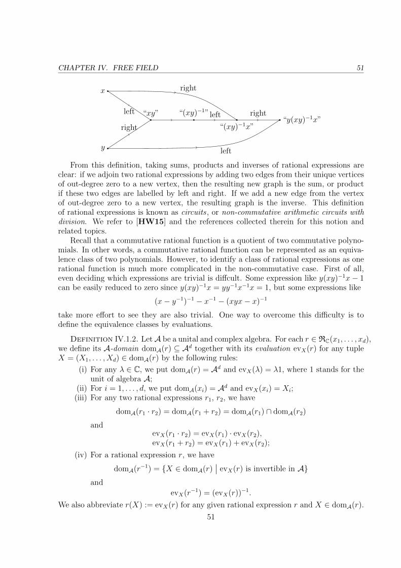
CHAPTER IV. FREE FIELD 51
x
y
“xy” “(xy)−1”
“(xy)−1x”“y(xy)−1x”
left
right
left right
right
left
From this definition, taking sums, products and inverses of rational expressions areclear: if we adjoin two rational expressions by adding two edges from their unique verticesof out-degree zero to a new vertex, then the resulting new graph is the sum, or productif these two edges are labelled by left and right. If we add a new edge from the vertexof out-degree zero to a new vertex, the resulting graph is the inverse. This definitionof rational expressions is known as circuits , or non-commutative arithmetic circuits withdivision. We refer to [HW15] and the references collected therein for this notion andrelated topics.
Recall that a commutative rational function is a quotient of two commutative polyno-mials. In other words, a commutative rational function can be represented as an equiva-lence class of two polynomials. However, to identify a class of rational expressions as onerational function is much more complicated in the non-commutative case. First of all,even deciding which expressions are trivial is diffcult. Some expression like y(xy)−1x− 1can be easily reduced to zero since y(xy)−1x = yy−1x−1x = 1, but some expressions like
(x− y−1)−1 − x−1 − (xyx− x)−1
take more effort to see they are also trivial. One way to overcome this difficulty is todefine the equivalence classes by evaluations.
Definition IV.1.2. LetA be a unital and complex algebra. For each r ∈ RC(x1, . . . , xd),we define its A-domain domA(r) ⊆ Ad together with its evaluation evX(r) for any tupleX = (X1, . . . , Xd) ∈ domA(r) by the following rules:
(i) For any λ ∈ C, we put domA(r) = Ad and evX(λ) = λ1, where 1 stands for theunit of algebra A;
(ii) For i = 1, . . . , d, we put domA(xi) = Ad and evX(xi) = Xi;(iii) For any two rational expressions r1, r2, we have
domA(r1 · r2) = domA(r1 + r2) = domA(r1) ∩ domA(r2)
andevX(r1 · r2) = evX(r1) · evX(r2),evX(r1 + r2) = evX(r1) + evX(r2);
(iv) For a rational expression r, we have
domA(r−1) = X ∈ domA(r)∣∣ evX(r) is invertible in A
and
evX(r−1) = (evX(r))−1.
We also abbreviate r(X) := evX(r) for any given rational expression r and X ∈ domA(r).
51
52 IV.2. NON-COMMUTATIVE RATIONAL FUNCTIONS
Therefore, we can define equivalence classes of rational expressions by the evaluationwhen a unital algebra A is given. That is, two rational expressions r1 and r2 are calledA-evaluation equivalent if domA(r1) ∩ domA(r2) 6= ∅ and r1(X) = r2(X) for all X ∈domA(r1) ∩ domA(r2). Of course there are many rational expressions that have emptydomain, such as 0−1 and (x − x)−1. If a rational expression has empty domain, we saythat it is degenerate. But here they are safely discarded when we consider the evaluationequivalence.
Then it remains to choose an appropriate algebra A if we want to define rational func-tions as A-evaluation equivalent classes of rational expressions. This approach was firstachieved by Amitsur [Ami66] by evaluating rational expressions on some large auxiliaryskew field. It turns out that the evaluation on matrices of all sizes is also sufficient, whichwas proved in [KV12].
IV.2. Non-commutative rational functions
In this section, we will introduce non-commutative rational functions, which constitutethe free field. It was already mentioned at the end of Section IV.1 that rational functionscan be constructed as evaluation equivalence classes of rational expressions . That gives usan intuitive way to understand rational functions but still does not answer the question:what are rational functions? In other words, we need a characterizing property of rationalfunctions which can be examined on what we have constructed.
So our first part in this section is to introduce some characterization property ofthe free field. Recall that in the commutative situation, such a characterization is notdifficult to state: the field of rational functions is the smallest field extending the algebraof commutative polynomials. However, non-commutative polynomials can be embeddedinto skew fields which are non-isomorphic; see [KV12] or [Coh85, Exercises 7.2] forsome examples. Hence it is not enough to characterize the skew field of non-commutativerational functions as the smallest skew field extending non-commutative polynomials.
It turns out that the missing property here is a universal property of the skew fieldof rational functions. In order to make this notion precise, we follow the terminologies in[Coh06, Section 7.2]. From now on, we will focus on the non-commutative case. So wewill skip the adjective “skew” when we talk about skew fields.
Definition IV.2.1. Let A be a ring.
(i) An A-ring is a ring K together with a homomorphism φ : A → K. In particular,if K is a field, then it will be called an A-field .
(ii) An A-field K with φ : A → K is called epic if K is generated by the image φ(A),i.e., there is no proper subfield of K containing φ(A).
(iii) An epic A-field K is called field of fractions of A if the homomorphism φ : A →K is injective.
Since we want to define some universal property for A-fields, we need to considerhomomorphisms which respect the A-field structure. So it is natural to consider an A-ring homomorphism, i.e., a homomorphism f from an A-ring K to another one L with thehomomorphisms φK : A → K and φL : A → L satisfying f φK = φL. However, since anynon-trivial homomorphism between fields must be injective, for an A-ring homomorphismf : K → L between two A-fields K and L, f(K) has to be a field containing (f φK)(A) =
52
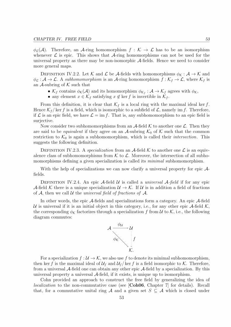
CHAPTER IV. FREE FIELD 53
φL(A). Therefore, an A-ring homomorphism f : K → L has to be an isomorphismwhenever L is epic. This shows that A-ring homomorphisms can not be used for theuniversal property as there may be non-isomorphic A-fields. Hence we need to considermore general maps.
Definition IV.2.2. Let K and L be A-fields with homomorphisms φK : A → K andφL : A → L. A subhomomorphism is an A-ring homomorphism f : Kf → L, where Kf isan A-subring of K such that
• Kf contains φK(A) and its homomorphism φKf: A → Kf agrees with φK,
• any element x ∈ Kf satisfying x 6∈ ker f is invertible in Kf .From this definition, it is clear that Kf is a local ring with the maximal ideal ker f .
Hence Kf/ ker f is a field, which is isomorphic to a subfield of L, namely im f . Therefore,if L is an epic field, we have L = im f . That is, any subhomomorphism to an epic field issurjective.
Now consider two subhomomorphisms from an A-field K to another one L. Then theyare said to be equivalent if they agree on an A-subring K0 of K such that the commonrestriction to K0 is again a subhomomorphism, which is called their intersection. Thissuggests the following definition.
Definition IV.2.3. A specialization from an A-field K to another one L is an equiv-alence class of subhomomorphisms from K to L. Moreover, the intersection of all subho-momorphisms defining a given specialization is called its minimal subhomomorphism.
With the help of specializations we can now clarify a universal property for epic A-fields.
Definition IV.2.4. An epic A-field U is called a universal A-field if for any epicA-field K there is a unique specialization U → K. If U is in addition a field of fractionsof A, then we call U the universal field of fractions of A.
In other words, the epic A-fields and specializations form a category. An epic A-fieldU is universal if it is an initial object in this category, i.e., for any other epic A-field K,the corresponding φK factorizes through a specialization f from U to K, i.e., the followingdiagram commutes:
A U
K.
φU
φK f
For a specialization f : U → K, we also use f to denote its minimal subhomomorphism,then ker f is the maximal ideal of Uf and Uf/ ker f is a field isomorphic to K. Therefore,from a universal A-field one can obtain any other epic A-field by a specialization. By thisuniversal property a universal A-field, if it exists, is unique up to isomorphism.
Cohn provided an approach to construct the free field by generalizing the idea oflocalization to the non-commutative case (see [Coh06, Chapter 7] for details). Recallthat, for a commutative unital ring A and a given set S ⊆ A which is closed under
53
54 IV.3. LINEAR REPRESENTATIONS
multiplication and contains 1, localization allows us to construct another ring AS togetherwith a homomorphism φ : A → AS such that all elements in the image φ(A) are invertiblein AS. Cohn discovered that one can replace the set S by a set of matrices Σ over Aand construct a universal localization AΣ, that is, a ring with a homomorphism φ : A →AΣ such that all elements in the image φ(Σ) are invertible in matrices over AΣ andany other ring with such a homomorphism can be factorized through AΣ. Moreover,if we take the set Σ to be the set of all full matrices over A and if Σ satisfies some“multiplicative closure” property, then this universal localization AΣ turns out to be theuniversal field of fractions of A. This closure property is called lower multiplicative; seethe paragraph before [Coh06, Proposition 7.1.1] for its definition. Actually, Cohn gives alist of characterizations for rings that can be embedded into universal fields of fractions.We select from this list the following items that are relevant for our purpose:
Theorem IV.2.5. (See [DS78] or [Coh06, Theorem 7.5.13]) Let A be any non-zeroring. We denote by Σ the set of all full matrices over A. Then the following conditionsare equivalent:
(i) A is a Sylvester domain.(ii) Σ is lower multiplicative.(iii) The universal localization AΣ is a field, necessarily the universal field of fractions
of A.(iv) A has an inner rank preserving homomorphism to the universal field of fractions
of A.
Recall that in Section III.2, the algebra C〈x1, . . . , xd〉 was shown to be a Sylvesterdomain; see Example III.2.4 and the discussion before it. Therefore, C〈x1, . . . , xd〉 canbe embedded into its universal field of fractions. We call this universal field of fractionsthe free field and denote it by C (<x1, . . . , xd )>. Naturally, an element in C (<x1, . . . , xd )>is called a rational function. Moreover, for a matrix A over polynomials, we do not needto distinguish between its inner rank over polynomials and its inner rank over rationalfunctions. This common inner rank is denoted by ρ(A) for a given matrix A.
IV.3. Linear representations
The localization in the last section tells us that a full matrix A over C〈x1, . . . , xd〉 isinvertible as a matrix over C (<x1, . . . , xd )>. So each entry in A−1 is a rational function.Therefore, for any row vector u and any column vector v over C, uA−1v is a rationalfunction since it is a linear combination of some rational functions. Actually, we add newelements more or less in this way to extend C〈x1, . . . , xd〉 to its universal localization,which turns out to be the free field C (<x1, . . . , xd )>. So one may expect that the converseshould be true, that is, any rational function r can be written in the form r = uA−1v,with some full matrix A over polynomials and two scalar-valued vectors u and v. Thisexpectation is indeed the case. Moreover, this matrix A can be chosen to be linear, thoughthe dimension of A may increase for exchange. This culminates in the following definitionborrowed from [CR99].
Definition IV.3.1. Let r be a rational function. A representation of a rationalfunction r is a tuple ρ = (u,A, v) consisting of a full matrix A ∈ Mn(C〈x1, . . . , xd〉), a
54
CHAPTER IV. FREE FIELD 55
row vector u ∈ M1,n(C) and a column vector Mn,1(C) such that r = uA−1v. Moreover,if the matrix A is linear (in the sense of Definition III.3.2), then we say ρ is a linearrepresentation of r.
In [CR99], such linear representations were used to give an alternative constructionof the free field. That indeed each element in the free field admits a linear representationis a direct consequence of the approach of [CR99]. But it also follows from the generaltheory presented in [Coh06]. The existence of a linear representation is an importantfeature for a rational function that will be used in Section V.2. So let us first we recordthe existence of linear representations for rational functions as a theorem.
Theorem IV.3.2. Each rational function r ∈ C (<x1, . . . , xd )> admits a linear repre-sentation in the sense of Definition IV.3.1.
The idea of realizing rational non-commutative functions by inverses of linear matriceshas been known for more than fifty years. It was rediscovered several times in manydifferent mathematical realms, such as automaton theory and non-commutative rationalseries, as well as computer science and engineering. Under the name “linearization trick”,it was introduced to the community of free probability by the work of Haagerup andThorbjørnsen [HT05] and Haagerup, Schultz, and Thorbjørnsen [HST06], building onearlier operator space versions; for the latter see in particular the work of Pisier [Pis18].
We will not include a detailed proof here for the above theorem. Instead we willshift our discussion to similar representations for rational expressions. In this way, wewill present an explicit algorithm to show how a linear matrix over non-commutativepolynomials can be constructed step by step to represent a concrete rational expression.
Actually, for the special case of non-commutative polynomials, similar concepts weredeveloped by Anderson [And12, And13, And15] and were used in [BMS17] in order tostudy evaluations of non-commutative polynomials in non-commutative random variablesby means of operator-valued free probability theory. Later, in [HMS18], these methodswere generalized to non-commutative rational expressions, based on a variant of DefinitionIV.3.1. We take this definition from [HMS18, Section 5], but with the sign changed forconvenience.
Definition IV.3.3. Let r be a rational expression in variables x1, . . . , xd. A formallinear representation ρ = (u,A, v) of r consists of a linear matrix A over C〈x1, . . . , xd〉, arow vector u and a column vector v over C such that for any unital algebra A,
domA(r) ⊆ X ∈ Ad∣∣ A(X) is invertible in A
and
r(X) = u(A(X))−1v
for any tuple X ∈ domA(r).
This definition asks that the inclusion of domA(r) (see Definition IV.1.2) into theset X ∈ Ad
∣∣ A(X) is invertible in A holds for arbitrary algebra A, but drops therequirement on the fullness of matrix A, in comparison to Definition IV.3.1. So clearlythese two representations are not the same objects. However, they have certain intrinsicconnections which will be exposed in the following.
55
56 IV.4. EVALUATION OF RATIONAL FUNCTIONS
First, let us give the explicit algorithm that builds a formal linear representation forany rational expression. We refer to [HMS18] for the motivation and the background forthe establishing of this algorithm.
Algorithm IV.3.4. A formal linear representation ρ = (u,A, v) of a rational expres-sion r can be constructed by using successively the following rules:
(i) For scalars λ ∈ C and the variables xj, j = 1, . . . , d, formal linear representa-tions are given by
ρλ := ((0 1
),
(−λ 11 0
),
(01
)),
and
ρxj := ((0 1
),
(−xj 1
1 0
),
(01
)).
(ii) If ρ1 = (u1, A1, v1) and ρ2 = (u2, A2, v2) are two formal linear representationsfor rational expressions r1 and r2, respectively, then
ρ1 ⊕ ρ2 := ((u1 u2
),
(A1 00 A2
),
(v1
v2
))
gives a formal linear representation of r1 + r2 and
ρ1 ρ2 := ((0 u1
),
(−v1u2 A1
A2 0
),
(0v2
))
gives a formal linear representation of r1 · r2.(iii) If ρ = (u,A, v) is a formal linear representation for rational expression r, then
ρ−1 := ((1 0
),
(0 uv A
),
(10
))
gives a formal linear representation of r−1.
A detailed proof for showing that this algorithm indeed produces formal linear repre-sentations can be found in [HMS18, Section 5] or [Mai17, Chapter III]. These formallinear representations are closely related to linear representations as introduced in Defi-nition IV.3.1. So this algorithm yields a perfect analogue of Theorem IV.3.2.
It may happen that the linear matrix A for a rational expression is not full, sincedegenerate rational expressions like 0−1 are allowed. However, for non-degenerate rationalexpressions, their formal linear representations automatically produce linear matrices Athat are full. This is explained in [Mai17, Chapter III]. Therefore, one can recover theexistence of linear representations for rational functions via formal linear representationsof rational expressions.
IV.4. Evaluation of rational functions
Let X = (X1, . . . , Xd) be a tuple of elements in a unital algebra A. Its evaluation mapevX from C〈x1, . . . , xd〉 to A is well-defined as a homomorphism. We have also seen thatthe evaluation of rational expressions can be defined naturally with A-domains consideredin Definition IV.1.2. Then the question is: how can we define the evaluation for rationalfunctions? Unfortunately, the evaluation cannot be well-defined for all algebras without
56
CHAPTER IV. FREE FIELD 57
additional assumptions. Here is an example which illustrates the problem: consideringA = B(H) for some infinite dimensional separable Hilbert space, let l denote the one-sided left-shift operator. Then l∗ is the right-shift operator and we have l · l∗ = 1 butl∗ · l 6= 1. It is clear that the evaluation of the rational expression r(x, y) = y(xy)−1xis r(l, l∗) = l∗l 6= 1. However, since this rational expression also represents the rationalfunction 1, there is no consistent way to define its value for the arguments l and l∗. So itis natural to consider algebras in which a left inverse is also a right inverse to avoid sucha problem. Actually, we require algebras to be stably finite in order to make sure that wehave a well-defined evaluation.
Theorem IV.4.1. Let A be a stably finite algebra. Then for any rational function rin the free field C (<x1, . . . , xd )>, we have a well-defined A-domain domA(r) ⊆ Ad and anevaluation r(X) for any X ∈ domA(r).
Actually, the converse also holds in some sense, see in [Coh06, Theorem 7.8.3] (oneshould note that the terminology there is quite different from ours). When rationalfunctions are treated as equivalence classes of rational expressions evaluated on matricesof all sizes, see also [HMS18, Theorem 6.1] for a proof of the same theorem. For thereader’s convenience, here we give a proof with the help of representations of rationalfunctions (introduced in Definition IV.3.1). Note we do not require the representationsto be linear here.
Definition IV.4.2. For a representation ρ = (u,A, v) of a rational function, we defineits A-domain
domA(ρ) = X ∈ Ad∣∣ A(X) is invertible as a matrix over A.
For a rational function r, we define its A-domain
domA(r) =⋃ρ
domA(ρ),
where the union is taken over all possible representations of r. Then we define the evalu-ation of r at a tuple X ∈ domA(r) by
EvX(r) = r(X) = u(A(X))−1v
for any representation ρ = (u,A, v) satisfying X ∈ domA(ρ).
Of course, as the choice of the representations for a rational function is not unique,we have to prove that different choices always give the same evaluation.
Proof of Theorem IV.4.1. Let ρ1 = (u1, A1, v1) and ρ2 = (u2, A2, v2) be two rep-resentations of a rational function r such that
r = u1A−11 v1 = u2A
−12 v2.
We need to prove that for any X ∈ domA(ρ1) ∩ domA(ρ2), we have u1(A1(X))−1v1 =u2(A2(X))−1v2. It is not difficult to verify that the tuple
((u1 u2
),
(A1 00 −A2
),
(v1
v2
))
57
58 IV.5. RATIONAL CLOSURES AND DIVISION CLOSURES
is a representation of zero in the free field. Hence it suffices to prove that, for anyrepresentation ρ = (u,A, v) of zero, we have u(A(X))−1v = 0 for any X ∈ domA(A).Now suppose that u(A(X))−1v 6= 0 for some representation ρ = (u,A, v) of the zerofunction. Then (
0 uv A(X)
)∈Mn+1(A)
has inner rank n+ 1 over A by Proposition III.1.6 as A is stably finite. However, we canapply the same proposition to show that(
0 uv A
)∈Mn+1(C〈x1, . . . , xd〉)
has inner rank n since uA−1v = 0 and C〈x1, . . . , xd〉 is stably finite. This gives an upperbound n for the inner rank of its evaluation by Item (v) of Remark III.1.3, because theevaluation of polynomials is always well-defined as a homomorphism. Hence we encountera contradiction and therefore we conclude that u(A(X))−1v = 0, as desired.
We close this section by remarking that this definition of evaluation is consistentwith the usual notion of evaluation. That is, given any polynomial p, in order to seethat the above definition coincides with the usual one, we should find a representationρ = (u,A, v) such that u(A(X))−1v equals p(X), the usual evaluation of p at X, for anyX ∈ Ad. Actually such a representation can be constructed by following the first tworules of Algorithm IV.3.4 for formal linear representations. Furthermore, from the lastrules of this algorithm, we can also see that the arithmetic operations between rationalfunctions give the corresponding arithmetic operations between their evaluations.
IV.5. Rational closures and division closures
In this section, we will introduce two constructions built by arithmetic operations(including taking inverses) from a given tuple of elements in an algebra. In general theyare not necessarily division rings like the free field. But they are algebras that have someproperty concerning the invertibility. They are called rational closure and division closure.Basically, rational closure is given by the possible evaluations of rational functions at agiven tuple. The division closure is the smallest algebra generated by a given tuple withrespect to a closure property of inverses. Our purpose of introducing them is to providethe underlying algebra over which the inner rank can be taken when we investigate thestrong Atiyah property in Section V.3.
Definition IV.5.1. Let X = (X1, . . . , Xd) be a tuple of elements in a unital algebraA. We denote by Σ the set of matrices whose evaluations at X are invertible, i.e.,
Σ =∞⋃n=1
A ∈Mn(C〈x1, . . . , xd〉)∣∣ A(X) is invertible in Mn(A).
The rational closure of X in A is the set of all entries of inverses of evaluations of Σ atX. We will denote this set by AX in the following.
We want to point out that the rational closure can be defined for more general setting,see [Coh06, Section 7.1]. In comparison to the general setting, we limit our considerationto the case that homomorphisms are given by evaluation maps induced by tuples over A.
58

CHAPTER IV. FREE FIELD 59
It is because this setting is exactly what we need later in Section V.3. However, even inthe general setting, we have the following lemma that tells us that the rational closure isalways an algebra.
Lemma IV.5.2. (See [Coh06, Proposition 7.1.1 and Theorem 7.1.2]) The rationalclosure AX is a subalgebra of A containing C〈X1, . . . , Xd〉, i.e., the image of C〈x1, . . . , xd〉under the evaluation homomorphism.
By definition, each element r ∈ AX is an entry of (A(X))−1 for some square matrix Aover C〈x1, . . . , xd〉 such that A(X) is invertible. Hence we can choose some scalar-valuedrow and column vectors u and v such that
r = u(A(X))−1v.
For example, if r is the (1, 1)-entry of (A(X))−1, then we can choose u = vT = (1, 0, . . . , 0)whose entries are all zero except the first one. Now if additionally A is stably finite, thenwe know that A(X) is a full matrix over A (by Proposition III.1.6). It follows that A is afull matrix according to Item (v) of Remark III.1.3. Therefore, we can regard (u,A, v) asa representation of the rational function uA−1v. Let us denote this rational function byf . So, according to Definition IV.4.2 and Theorem IV.4.1, we see that r = f(X). Thatis, each element in AX is given by the evaluation of some rational function. Conversely,if a rational function f has a well-defined evaluation f(X), then there exist a full matrixA and scalar-valued row and column vectors u and v such that A(X) is invertible andf(X) = u(A(X))−1v. That is, we can write f(X) as a linear combination of entries of(A(X))−1. So f(X) has to be in the rational closure AX since AX is an algebra (due toLemma IV.5.2). In other words, the rational closure of X in A is the set of all well-definedevaluations of rational functions. We record this fact as the following remark.
Remark IV.5.3. Let X = (X1, . . . , Xd) be a tuple of elements in a stably finite algebraA. Then we have
AX = r(X) ∈ A∣∣ r ∈ C (<x1, . . . , xd )>, r(X) is well defined.
In general, for a given tuple X, the rational closure AX may not be a division ring ingeneral. But it has a property concerning inverses: if an element r ∈ AX is invertible inA, then r−1 ∈ AX . Actually, this can be seen from the last item in Algorithm IV.3.4: ifr = u(A(X))−1v for some matrix A over C〈x1, . . . , xd〉 and scalar-valued row and columnvectors u and v, then
r−1 =(1 0
)(0 uv A(X)
)−1(10
),
where the invertiblity of matrix (0 uv A(X)
)follows from the invertiblity of r = u(A(X))−1v in A by the following well-known lemmaon Schur complements.
Lemma IV.5.4. Suppose that A is a unital algebra. Let m,n be positive integers,A ∈ Mm(A), B ∈ Mm×n(A), C ∈ Mn×m(A) and D ∈ Mn(A) such that D is invertible.
59
60 IV.5. RATIONAL CLOSURES AND DIVISION CLOSURES
Then the matrix (A BC D
)is invertible in Mm+n(A) if and only if the Schur complement A − BD−1C is invertiblein Mm(A).
A closely related notion is the smallest subalgebra satisfying this property, see [Coh85,Exercises 7.1.4] or [Coh06, Exercise 7.1.3].
Definition IV.5.5. Let B be a subalgebgra of a unital algebra A.
(i) B is called division closed if for every a ∈ B that is invertible in A the inversea−1 lies in B.
(ii) The division closure (or unit-closure) of B in A is the smallest division closedsubalgebra of A containing B. We denote it by C (<B )>.In particular, we denote the division closure of C〈X1, . . . , Xd〉 by C (<X1, . . . , Xd )>for a given tuple X = (X1, . . . , Xd) over A.
Remark IV.5.6. Let A be a unital algebra. We have the following remarks in order.
(i) Let B be a division closed subalgebra of A. If every non-zero a ∈ B is invertiblein A, then B is a division ring.
(ii) Let X = (X1, . . . , Xd) be a tuple of elements in A. Then the rational closureAX contains the division closure C (<X1, . . . , Xd )> since AX is division closed.
(iii) In particular, one can set A = C (<x1 . . . , xd )> and choose B = C〈x1 . . . , xd〉.Naturally, one would expect that
C (<C〈x1 . . . , xd〉 )> = C (<x1 . . . , xd )>.
In order to see this, note that C (<C〈x1 . . . , xd〉 )> becomes a division ring accord-ing to the Item (i) of this remark. Then the result follows from the fact thatC (<x1 . . . , xd )> is epic (see Definition IV.2.1).
(iv) Let B be a subalgebra of A. Then its division closure C (<B )> has a recursivestructure as follows. We denote R0(B) := B and set
R−10 (B) := a−1
∣∣ a ∈ R0(B), a is invertible in A.
Clearly we have R−10 (B) ⊆ C (<B )>. Next we define R1(B) as the subalgebra of A
generated by R0(B) and R−10 (B), i.e., the smallest subalgebra of A containing
R0(B) ∪ R−10 (B). Then R1(B) ⊆ C (<B )> since R0(B) ∪ R−1
0 (B) ⊆ C (<B )>.Applying this procedure iteratively yields a sequence (Rk(B))∞k=0 of subalgebrasof C (<B )> that each Rk(B) is generated by Rk−1(B) and R−1
k−1(B). Therefore,we define
R∞(B) :=∞⋃k=0
Rk(B)
which also belongs to C (<B )>. Actually, for any division closed subalgebra D ofA containing B, we have R∞(B) ⊆ D. Moreover, R∞(B) is also division closed.It is because that for any r ∈ Rk(B) we have r−1 ∈ Rk+1(B) if it exists in A. Inconclusion, R∞(B) is the smallest division closed subalgebgra of A containingB, namely, R∞(B) = C (<B )>.
60
CHAPTER IV. FREE FIELD 61
In general, the division closure may not equal to the rational closure. However, theycould agree with each other in some cases. Here we provide a case that we will meet inSection V.3.
Proposition IV.5.7. Let X = (X1, . . . , Xd) be a tuple of elements in A. If therational closure AX or the division closure C (<X1, . . . , Xd )> is a division ring, then AX =C (<X1, . . . , Xd )>.
Proof. If AX is a division ring, then C (<X1, . . . , Xd )> is also a division ring dueto Item (i) of Remark IV.5.6. Therefore, it suffices to show that if C (<X1, . . . , Xd )> is adivision ring then AX = C (<X1, . . . , Xd )>. Let r be an element in AX . Then there exists amatrix A over C〈x1, . . . , xd〉 such that A(X) is invertible as matrix overA and r is an entryof (A(X))−1. So our proposition will follow if (A(X))−1 is a matrix over C (<X1, . . . , Xd )>.Actually, we can prove that for any n ∈ N+, Mn(C (<X1, . . . , Xd )>) is division closed inMn(A). Therefore, the proof will be completed by the following lemma.
Lemma IV.5.8. Let D be a subalgebra of A. If D is a division ring, then Mn(D) isdivision closed in Mn(A) for any n ∈ N+.
Proof. We are going to prove this by induction on the size n of matrices. First, theresult clearly holds for n = 1 since D is division closed. Now we assume that the resultis true for matrices of size n − 1. Let A ∈ Mn(D) be invertible in Mn(A). Then we canwrite
A =
(B cd e
),
where B ∈ Mn−1(D) and c, d and e are of appropriate size such that e 6= 0. (We mightneed to apply row and column permutations to make sure that e 6= 0.) Note that eis invertible in D since D is a division ring. We see that B − ce−1d lies in Mn−1(D).Moreover, B− ce−1d is invertible in Mn−1(A) by Lemma IV.5.4 as A and e are invertible.By the induction hypothesis, it follows that (B − ce−1d)−1 ∈Mn−1(D). Finally, from theequation
A−1 =
(1n−1 0−e−1d 1
)((B − ce−1d)−1 0
0 e−1
)(1n−1 −ce−1
0 1
)we see that A−1 ∈Mn(D). This completes the proof.
As a remark, we point out that the assumption in Proposition IV.5.7 can be weakened.For example, [Rei06, Note 13.16] says that if the division closure is a von Neumann regularring then it coincides with the rational closure.
In Section V.3, we will answer the question when the rational closure AX or divisionclosure C (<X1, . . . , Xd )> becomes a division ring for a tuple X of non-commutative randomvariables. In that case, Proposition IV.5.7 tell us that we don’t need to distinguish therational closure and division closure.
61


CHAPTER V
Atiyah property
In [Ati76], Atiyah extended the Atiyah-Singer index theorem to some non-compactmanifolds. He showed that using a dimension of a module over a von Neumann algebracan lead to a finite index though the kernel in question is in general infinite dimensional.This version is called the L2-index theorem as square integrability is imposed to give somegrowth condition. He also asked whether some analytic L2-Betti numbers are always ra-tional numbers for certain Riemannian manifolds. An answer can be given by consideringthe corresponding strong Atiyah conjecture for certain groups. We refer the interestedreader to [Luc02, Chapter 10] or [GLSZ00, DLM+03, PT11] for its precise statementand relevant literature.
Our exposition of this chapter will convey a perspective from free probability theory,based on [MSY18, MSY19]. In the context of free probability, Shlyakhtenko and Sk-oufranis introduced the strong Atiyah property for ∗-algebras of bounded operators withtracial vector states. We follow their notion with some adaptation:
Definition V.0.1. ([SS15, Definition 2.1]) Let X = (X1, . . . , Xd) be a tuple of ran-dom variables from a tracial W ∗-probability space (M, ϕ) and let evX : C〈x1, . . . , xd〉 →M be the evaluation homomorphism. If for any n ∈ N+ and matrixA ∈Mn(C〈x1, . . . , xd〉),we have
rank(A(X)) ∈ N,where rank : Mn(M)→ [0, n] is a rank function that measures the size of the image of anelement in Mn(M) (see Definition I.5.10), then we say X has the strong Atiyah property .
Linnell proved in [Lin93] that the free group satisfies the strong Atiyah conjecture.In other words, a tuple of freely independent Haar unitary random variables has thestrong Atiyah property in the sense of Definition V.0.1. This result was extended to moregeneral random variables by Shlyakhtenko and Skoufranis in [SS15] in the context of freeprobability. That is, they proved that a tuple of freely independent random variables withnon-atomic distributions has the strong Atiyah property.
These random variables turn out to have a stronger property which implies the strongAtiyah property. This property is, roughly speaking, the following: a tuple of freelyindependent random variables with non-atomic distributions can realize the free field inthe ∗-algebra of affiliated operators. In fact, this property was known for free groups in thecontext of Atiyah conjecture. Linnell showed in [Lin93] that the free group can realize thefree field in the ∗-algebra of affiliated operators. Restricted to the group case, there are noother groups that can realize the free field besides free groups. But when it comes to freelyindependent random variables with non-atomic distributions, there is a lot of freedomto choose different distributions (for example, semicircular distributions). However, thechoices of distributions might make no differences for the purpose of realizing the free
63
64 V.1. MAXIMALITY OF ∆
field. This is indeed the case that was confirmed by [MSY18]. Detailed discussion on therealization of the free field will be given in Section V.2. But instead of considering freelyindependent random variables with non-atomic distributions, we will consider randomvariables satisfying weaker properties. It will be explained in Section VI.1 why freelyindependent random variables with non-atomic distributions satisfy these properties.
In Section V.1, we will introduce a quantity ∆ due to Connes and Shlyakhtenko . Thepurpose of their article [CS05] was to study the L2-homology for von Neumann algebras.Along the way they found this quantity ∆ that behaves very similarly to Voiculescu’sfree entropy dimension. Moreover, they also showed an inequality between ∆ and somevariant of the free entropy dimension. From this it can be deduced that freely independentrandom variables with non-atomic distributions maximize ∆ (see Section VI.1 for details).In our investigation, we regard the maximality of ∆ as a property that characterizes atuple of random variables. Our goal of the first section in this chapter is to show that themaximality of ∆ is equivalent to the triviality of kernels of linear full matrices.
In Section V.2, we will extend the list of equivalent properties in the first section to amuch longer one. In particular, we will include the realization of the free field as one ofthose equivalent properties in our full list. In order to do that, two key ideas from ChapterIII and Chapter IV are applied. First, the linear representation of rational functions willbe used to transfer our results about the invertibility from matrices over polynomials torational functions. Secondly, the diagonalization of matrices over polynomials by rationalfunctions will be used to reveal an equality between the inner rank over over polynomialsand the analytic rank over von Neumann algebra. This equality in turn implies that fullmatrices have trivial kernels.
In Section V.3, we will come back to examine the strong Atiyah property with ideassimilar to Section V.2. Namely, we will show an analogue of our list of equivalent proper-ties as in Theorem V.2.2. In particular, we will show that a tuple X has the strong Atiyahproperty if and only if for any matrix A over C〈x1, . . . , xd〉, rank(A(X)) equals to the innerrank of A(X) taken over the rational closure of X. This equality enforces rank(A(X)) tobe an integer for any matrix A, so it clearly implies the strong Atiyah property. Note thatby definition the strong Atiyah property only asks rank(A(X)) to take values in integerswithout specification to any quantity. We thus give an algebraic reason why the analyticrank in the strong Atiyah property only takes values in integers. Such an equality for thestrong Atiyah property or strong Atiyah conjecture was not known until [MSY18] as faras the author’s knowledge.
V.1. Maximality of ∆
This section is based on [MSY19, Section 3]. In comparison to [MSY18], it containsthe major new idea that the entropy dimension used in [MSY18] can be replaced by thequantity ∆. With the help of ∆, new methods can be introduced (as we will see in thissection) to get much stronger results than [MSY18].
We will first introduce the quantity ∆(X) for a tuple X = (X1, . . . , Xd) of randomvariables. Our goal is show that ∆(X) = d if and only if ker(A(X)) = 0 for all linearfull matrix A over C〈x1, . . . , xd〉. To achieve that purpose, we will need a third equivalentproperty for X. This property drops the notion of the fullness but instead addresses the
64
CHAPTER V. ATIYAH PROPERTY 65
linear dependence of vectors in kernels. We will actually prove that this third property isequivalent to the previous two properties respectively.
The main proof will be given as the second subsection. In the first subsection, we willpresent two key lemmas. Moreover, these two lemmas might be of independent interestsince they provide explicit constructions that connect ∆ and linear matrices with kernelvectors.
Now, let (M, ϕ) be a tracial W ∗-probability space and let X = (X1, . . . , Xd) be atuple of random variables in M. A quantity ∆(X) was introduced in [CS05] as
(V.1) ∆(X) := d− dimM⊗Mop
(T1, . . . , Td) ∈ (F(L2(M, ϕ)))d
∣∣ d∑k=1
[Tk, JXkJ ] = 0HS
.
Here, we denote by F(L2(M, ϕ)) the ideal of all finite rank operators on L2(M, ϕ).Tomita’s conjugation operator J : L2(M, ϕ) → L2(M, ϕ) is the conjugate-linear mapthat extends isometrically the conjugation x 7→ x∗ on M. The closure of these tuples offinite rank operators is taken with respect to the Hilbert-Schmidt norm. The dimensionfunction used here is the dimension function introduced by Luck, see [Luc02, Section6.1].
Our main result is the following list of equivalent descriptions for the maximality of∆(X) with the help of linear matrices C〈x1, . . . , xd〉.
Theorem V.1.1. Let (M, ϕ) be a tracial W ∗-probability space. For a tuple X =(X1, . . . , Xd) of random variables in M, the following are equivalent:
(i) ∆(X) = d.(ii) For any n ∈ N+ and non-zero linear matrix A ∈ Mn(C〈x1, . . . , xd〉), if f ∈
ker(A(X)), e ∈ ker((A(X))∗), then either e or f has linearly dependent compo-nents.
(iii) For any n ∈ N+ and linear full matrix A ∈Mn(C〈x1, . . . , xd〉), ker(A(X)) = 0.
Remark V.1.2. Before giving the proof, the following remarks are in order.
(i) Suppose that ∆(X1, . . . , Xd) < d. By definition, this means that there is a tuple(T1, . . . , Td) 6= (0, . . . , 0) of finite rank operators in B(L2(M, ϕ)) with the prop-
erty that∑d
k=1[Tk, JXkJ ] = 0. We infer from the latter that (JT1J, . . . , JTdJ),which is again a non-trivial tuple of finite rank operators on L2(M, ϕ), satisfies∑d
k=1[JTkJ,Xk] = 0.(ii) In Item (ii) of Theorem V.1.1, the random variable (A(X))∗ will be frequently
rewritten as(A(X))∗ = A∗(X∗),
where X∗ := (X∗1 , . . . , X∗d) and A∗ is understood in the sense of Item (iv) of Def-
inition I.2.1. Namely, the ∗-structure on C〈x1, . . . , xd〉 is determined by 1∗ = 1and x∗k = xk for k = 1, . . . , d. Note that we usually use this ∗-structure onC〈x1, . . . , xd〉 if the tuple X consists of self-adjoint random variables. Of coursehere the random variables X1, . . . , Xd may not be self-adjoint. But we can-not use the evaluation homomorphism ev : C 〈x1, . . . , xd, x
∗1 . . . , x
∗d〉 →M given
in Item (v) of Definition I.2.1. This is because there might be relations be-tween Xk and X∗k for some k, for example, XkX
∗k = X∗kXk = 1. However,
65
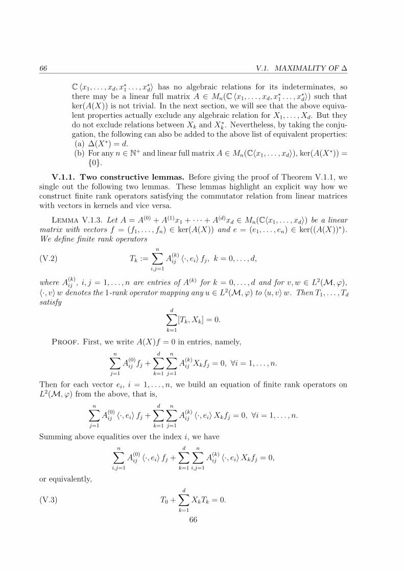
66 V.1. MAXIMALITY OF ∆
C 〈x1, . . . , xd, x∗1 . . . , x
∗d〉 has no algebraic relations for its indeterminates, so
there may be a linear full matrix A ∈ Mn(C 〈x1, . . . , xd, x∗1 . . . , x
∗d〉) such that
ker(A(X)) is not trivial. In the next section, we will see that the above equiva-lent properties actually exclude any algebraic relation for X1, . . . , Xd. But theydo not exclude relations between Xk and X∗k . Nevertheless, by taking the conju-gation, the following can also be added to the above list of equivalent properties:(a) ∆(X∗) = d.(b) For any n ∈ N+ and linear full matrixA ∈Mn(C〈x1, . . . , xd〉), ker(A(X∗)) =0.
V.1.1. Two constructive lemmas. Before giving the proof of Theorem V.1.1, wesingle out the following two lemmas. These lemmas highlight an explicit way how weconstruct finite rank operators satisfying the commutator relation from linear matriceswith vectors in kernels and vice versa.
Lemma V.1.3. Let A = A(0) + A(1)x1 + · · · + A(d)xd ∈ Mn(C〈x1, . . . , xd〉) be a linearmatrix with vectors f = (f1, . . . , fn) ∈ ker(A(X)) and e = (e1, . . . , en) ∈ ker((A(X))∗).We define finite rank operators
(V.2) Tk :=n∑
i,j=1
A(k)ij 〈·, ei〉 fj, k = 0, . . . , d,
where A(k)ij , i, j = 1, . . . , n are entries of A(k) for k = 0, . . . , d and for v, w ∈ L2(M, ϕ),
〈·, v〉w denotes the 1-rank operator mapping any u ∈ L2(M, ϕ) to 〈u, v〉w. Then T1, . . . , Tdsatisfy
d∑k=1
[Tk, Xk] = 0.
Proof. First, we write A(X)f = 0 in entries, namely,
n∑j=1
A(0)ij fj +
d∑k=1
n∑j=1
A(k)ij Xkfj = 0, ∀i = 1, . . . , n.
Then for each vector ei, i = 1, . . . , n, we build an equation of finite rank operators onL2(M, ϕ) from the above, that is,
n∑j=1
A(0)ij 〈·, ei〉 fj +
d∑k=1
n∑j=1
A(k)ij 〈·, ei〉Xkfj = 0, ∀i = 1, . . . , n.
Summing above equalities over the index i, we have
n∑i,j=1
A(0)ij 〈·, ei〉 fj +
d∑k=1
n∑i,j=1
A(k)ij 〈·, ei〉Xkfj = 0,
or equivalently,
(V.3) T0 +d∑
k=1
XkTk = 0.
66

CHAPTER V. ATIYAH PROPERTY 67
Similarly, from (A(X))∗e = 0, i.e.,
n∑j=1
A(0)ji ej +
d∑k=1
n∑j=1
A(k)ji X
∗kej = 0, ∀i = 1, . . . , n,
we haven∑j=1
⟨·, A(0)
ji ej
⟩fi +
d∑k=1
n∑j=1
⟨·, A(k)
ji X∗kej
⟩fi = 0, ∀i = 1, . . . , n,
which yieldsn∑
i,j=1
A(0)ji 〈·, ej〉 fi +
d∑k=1
n∑i,j=1
A(k)ji 〈Xk·, ej〉 fi = 0.
Actually, that is
(V.4) T0 +d∑
k=1
TkXk = 0.
Therefore, combining (V.3) and (V.4), we conclude that∑d
k=1[Tk, Xk] = 0.
Lemma V.1.4. Suppose that X = (X1, . . . , Xd) is a tuple of random variables in Mand (T1, . . . , Td) is a tuple of finite rank operators on L2(M, ϕ) satisfying
(V.5)d∑
k=1
[Tk, Xk] = 0.
Let f = (f1, . . . , fn) be an orthonormal family which spans the space of the sum of sub-spaces imTk + imT ∗k , k = 1, . . . , d. We write each Tk as
(V.6) Tk =n∑
i,j=1
A(k)ij 〈·, fi〉 fj, k = 1, . . . , d.
Then the linear matrix
(V.7) A := A(0) − A(1)x1 + · · ·+ A(d)xd,
where A(k) := (A(k)ij )ni,j=1 ∈Mn(C), k = 1, . . . , d,
B(k) := (〈Xkfi, fj〉)ni,j=1, k = 1 . . . , d, and A(0) :=d∑
k=1
B(k)A(k),
satisfies
A(X)f = 0 and A(X)∗f = 0.
Proof. Substituting the form of Tk, k = 1, . . . , d in (V.6) into the relation (V.5), wehave
d∑k=1
n∑i,j=1
A(k)ij 〈Xk·, fi〉 fj =
d∑k=1
n∑i,j=1
A(k)ij 〈·, fi〉Xkfj.
67
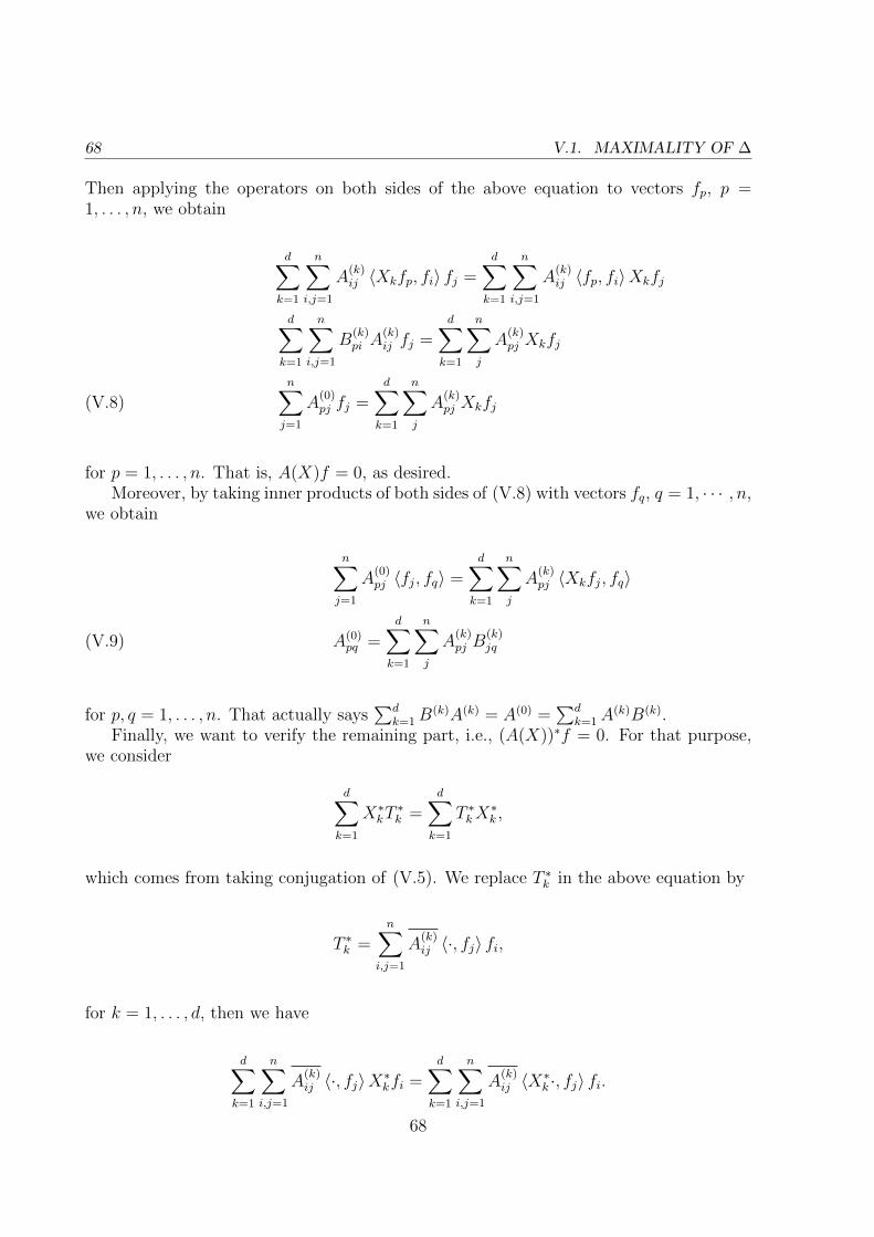
68 V.1. MAXIMALITY OF ∆
Then applying the operators on both sides of the above equation to vectors fp, p =1, . . . , n, we obtain
d∑k=1
n∑i,j=1
A(k)ij 〈Xkfp, fi〉 fj =
d∑k=1
n∑i,j=1
A(k)ij 〈fp, fi〉Xkfj
d∑k=1
n∑i,j=1
B(k)pi A
(k)ij fj =
d∑k=1
n∑j
A(k)pj Xkfj
n∑j=1
A(0)pj fj =
d∑k=1
n∑j
A(k)pj Xkfj(V.8)
for p = 1, . . . , n. That is, A(X)f = 0, as desired.Moreover, by taking inner products of both sides of (V.8) with vectors fq, q = 1, · · · , n,
we obtain
n∑j=1
A(0)pj 〈fj, fq〉 =
d∑k=1
n∑j
A(k)pj 〈Xkfj, fq〉
A(0)pq =
d∑k=1
n∑j
A(k)pj B
(k)jq(V.9)
for p, q = 1, . . . , n. That actually says∑d
k=1B(k)A(k) = A(0) =
∑dk=1A
(k)B(k).Finally, we want to verify the remaining part, i.e., (A(X))∗f = 0. For that purpose,
we consider
d∑k=1
X∗kT∗k =
d∑k=1
T ∗kX∗k ,
which comes from taking conjugation of (V.5). We replace T ∗k in the above equation by
T ∗k =n∑
i,j=1
A(k)ij 〈·, fj〉 fi,
for k = 1, . . . , d, then we have
d∑k=1
n∑i,j=1
A(k)ij 〈·, fj〉X∗kfi =
d∑k=1
n∑i,j=1
A(k)ij 〈X∗k ·, fj〉 fi.
68
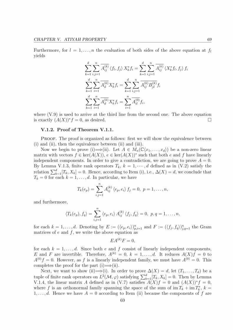
CHAPTER V. ATIYAH PROPERTY 69
Furthermore, for l = 1, . . . , n the evaluation of both sides of the above equation at flyields
d∑k=1
n∑i,j=1
A(k)ij 〈fl, fj〉X∗kfi =
d∑k=1
n∑i,j=1
A(k)ij 〈X∗kfl, fj〉 fi
d∑k=1
n∑i=1
A(k)il X
∗kfi =
d∑k=1
n∑i,j=1
A(k)ij B
(k)jl fi
d∑k=1
n∑i=1
A(k)il X
∗kfi =
n∑i=1
A(0)il fi,
where (V.9) is used to arrive at the third line from the second one. The above equationis exactly (A(X))∗f = 0, as desired.
V.1.2. Proof of Theorem V.1.1.
Proof. The proof is organized as follows: first we will show the equivalence between(i) and (ii), then the equivalence between (ii) and (iii).
Now we begin to prove (i)=⇒(ii). Let A ∈ Mn(C〈x1, . . . , xd〉) be a non-zero linearmatrix with vectors f ∈ ker(A(X)), e ∈ ker(A(X))∗ such that both e and f have linearlyindependent components. In order to give a contradiction, we are going to prove A = 0.By Lemma V.1.3, finite rank operators Tk, k = 1, · · · , d defined as in (V.2) satisfy the
relation∑d
k=1[Tk, Xk] = 0. Hence, according to Item (i), i.e., ∆(X) = d, we conclude thatTk = 0 for each k = 1, . . . , d. In particular, we have
Tk(ep) =n∑
i,j=1
A(k)ij 〈ep, ei〉 fj = 0, p = 1, . . . , n,
and furthermore,
〈Tk(ep), fq〉 =n∑
i,j=1
〈ep, ei〉A(k)ij 〈fj, fq〉 = 0, p, q = 1, . . . , n,
for each k = 1, . . . , d. Denoting by E := (〈ep, ei〉)np,i=1 and F := (〈fj, fq〉)nj,q=1 the Grammatrices of e and f , we write the above equation as
EA(k)F = 0,
for each k = 1, . . . , d. Since both e and f consist of linearly independent components,E and F are invertible. Therefore, A(k) = 0, k = 1, . . . , d. It reduces A(X)f = 0 toA(0)f = 0. However, as f is a linearly independent family, we must have A(0) = 0. Thiscompletes the proof for the part (i)=⇒(ii).
Next, we want to show (ii)=⇒(i). In order to prove ∆(X) = d, let (T1, . . . , Td) be a
tuple of finite rank operators on L2(M, ϕ) satisfying∑d
k=1[Tk, Xk] = 0. Then by LemmaV.1.4, the linear matrix A defined as in (V.7) satisfies A(X)f = 0 and (A(X))∗f = 0,where f is an orthonormal family spanning the space of the sum of imTk + imT ∗k , k =1, . . . , d. Hence we have A = 0 according to Item (ii) because the components of f are
69
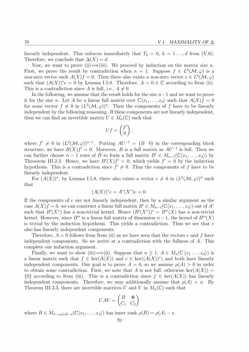
70 V.1. MAXIMALITY OF ∆
linearly independent. This enforces immediately that Tk = 0, k = 1 . . . , d from (V.6).Therefore, we conclude that ∆(X) = d.
Now, we want to prove (ii)=⇒(iii). We proceed by induction on the matrix size n.First, we prove the result by contradiction when n = 1. Suppose f ∈ L2(M, ϕ) is anon-zero vector such A(X)f = 0. Then there also exists a non-zero vector e ∈ L2(M, ϕ)such that (A(X))∗e = 0 by Lemma I.5.8. Therefore, A = 0 ∈ C according to Item (ii).This is a contradiction since A is full, i.e., A 6= 0.
In the following, we assume that the result holds for the size n−1 and we want to proveit for the size n. Let A be a linear full matrix over C〈x1, . . . , xd〉 such that A(X)f = 0for some vector f 6= 0 in (L2(M, ϕ))n. Then the components of f have to be linearlyindependent by the following reasoning. If these components are not linearly independent,then we can find an invertible matrix U ∈Mn(C) such that
Uf =
(f ′
0
),
where f ′ 6= 0 in (L2(M, ϕ))n−1. Putting AU−1 =(B b
)in the corresponding block
structure, we have B(X)f ′ = 0. Moreover, B is a full matrix as AU−1 is full. Then wecan further choose n − 1 rows of B to form a full matrix B′ ∈ Mn−1(C〈x1, . . . , xd〉) byTheoerem III.2.3. Hence, we have B′(X)f ′ = 0, which yields f ′ = 0 by the inductionhypothesis. This is a contradiction since f ′ 6= 0. Thus the components of f have to belinearly independent.
For (A(X))∗, by Lemma I.5.8, there also exists a vector e 6= 0 in (L2(M, ϕ))n suchthat
(A(X))∗e = A∗(X∗)e = 0.
If the components of e are not linearly independent, then by a similar argument as thecase A(X)f = 0, we can construct a linear full matrix B′ ∈Mn−1(C〈x1, . . . , xd〉) out of A∗
such that B′(X∗) has a non-trivial kernel. Hence (B′(X∗))∗ = B′∗(X) has a non-trivialkernel. However, since B′∗ is a linear full matrix of dimension n− 1, the kernel of B′∗(X)is trivial by the induction hypothesis. This yields a contradiction. Thus we see that ealso has linearly independent components.
Therefore, A = 0 follows from Item (ii) as we have seen that the vectors e and f haveindependent components. So we arrive at a contradiction with the fullness of A. Thiscomplete our induction argument.
Finally, we want to show (iii)=⇒(ii). Suppose that n ≥ 1, A ∈ Mn(C 〈x1 . . . , xd〉) isa linear matrix such that f ∈ ker(A(X)) and e ∈ ker((A(X))∗) and both have linearlyindependent components. Our goal is to prove A = 0, so we assume ρ(A) > 0 in orderto obtain some contradiction. First, we note that A is not full, otherwise ker(A(X)) =0 according to Item (iii). This is a contradiction since f ∈ ker(A(X)) has linearlyindependent components. Therefore, we may additionally assume that ρ(A) < n. ByTheorem III.3.3, there are invertible matrices U and V in Mn(C) such that
UAV =
(B 0C1 C2
)where B ∈Mn−s,ρ(A)−s(C〈x1, . . . , xd〉) has inner rank ρ(B) = ρ(A)− s.
70
CHAPTER V. ATIYAH PROPERTY 71
If s < ρ(A), i.e., the block B does not disappear in the above form of UAV , then letus write
V −1f =
(f ′
f ′′
),
where f ′ ∈ (L2(M, ϕ))ρ(A)−s. Clearly we have B(X)f ′ = 0 and we consider this equationrather than A(X)f = 0. By consulting Theorem III.2.3, we can choose ρ(A) − s rowsof B to form a linear full matrix B′ ∈ Mρ(A)−s(C〈x1, . . . , xd〉). It then follows thatB′(X)f ′ = 0. Thus f ′ = 0 according to Item (iii). However, this is impossible since f haslinearly independent components and V ∈Mn(C) is invertible.
So it remains to deal with the case that s = ρ(A). In this case, Theorem III.3.3actually says that
UAV =
(0C2
),
where C2 ∈Mρ(A),n(C〈x1, . . . , xd〉). From (A(X))∗e = 0, we see that
(UAV )∗(X∗)(U∗)−1e = V ∗A∗(X∗)U∗(U∗)−1e = V ∗(A(X))∗e = 0.
That is, (0 C∗2(X∗)
)(U∗)−1e = 0.
Similarly, we can build out of C∗2 a linear full matrix which has non-trivial kernel. Thisgives a contradiction as desired.
Therefore, we rule out the possibility that ρ(A) 6= 0 when there are vectors e and fthat have linearly independent components. This completes the proof for the last part ofour theorem.
V.2. Realization of the free field
In this section, we will extend the list of equivalent properties in Theorem V.1.1.Actually, we will give another list of equivalent properties for a tuple of random variables.Of course these two lists have a common item. The reason that we separate these two listsis that they rely on very different ideas. We have seen that Theorem V.1.1 relies on ourtwo constructive lemmas to associate finite rank operators to linear matrices with vectorsin kernels. However, we will not need to deal with these notions in this section any more.Instead, a more algebraic idea will dominate the proof of the coming theorem. In otherwords, we have delved into questions on the vectors in L2(M, ϕ) in the last section, butfrom now on we will instead consider objects in L0(M, ϕ). Recall that L0(M, ϕ) is the∗-algebra of all unbounded random variables, see Section I.5. The first important fact isthat we can evaluate rational functions on this algebra L0(M, ϕ).
As we want to evaluate rational functions on L0(M, ϕ), we have to show that L0(M, ϕ)is stably finite. (Note that we always require that ϕ is a trace to consider L0(M, ϕ).)This fact is probably well-known to experts. We refer the interested reader to [HMS18,MSY19] for a proof. We simply record it as the following remark.
Remark V.2.1. L0(M, ϕ) is stably finite and thus the evaluation of rational functionsas in Definition IV.4.2 is well-defined on L0(M, ϕ).
71
72 V.2. REALIZATION OF THE FREE FIELD
Another important fact about L0(M, ϕ) is that we can rephrase the triviality of kernelsby the invertibility in L0(M, ϕ) (see Lemma I.5.9). With this rephrasing, we will see thatmany algebraic tools become available. Moreover, the invertibility is also characterizedby the maximality of the analytic rank function given in Definition I.5.10. Recall thatLemma I.5.11 says that any A ∈ Mn(L0(M, ϕ)) is invertible if and only if rank(A) = n.Then Item (iii) in Theorem V.1.1 can be rephrased as follows:
For any n ∈ N+ and linear matrix A ∈Mn(C〈x1, . . . , xd〉), if ρ(A) = n,then rank(A(X)) = n.
Compare this to the strong Atiyah property (Definition V.0.1) which requires that for anymatrix A ∈Mn(C〈x1, . . . , xd〉) we have rank(A(X)) ∈ N. One may ask whether we couldfurther have rank(A(X)) = ρ(A), which in particular implies that rank(A(X)) ∈ N. Wewill show that this equality is actually an equivalent property in our list.
Now we have all the ingredients to state our theorem. Note that the first item is exactlyItem (iii) in Theorem V.1.1 (with the triviality of kernels rephrased by the invertibility).
Theorem V.2.2. Let (M, ϕ) be a tracial W ∗-probability space and L0(M, ϕ) the ∗-algebra of unbounded random variables. For a given tuple X = (X1, . . . , Xd) in Mn,we consider the evaluation homomorphism evX : C〈x1, . . . , xd〉 → L0(M, ϕ). Then thefollowing properties for X are equivalent.
(i) For any n ∈ N+ and linear full matrix A ∈Mn(C〈x1, . . . , xd〉), A(X) is invertiblein Mn(L0(M, ϕ)).
(ii) For any n ∈ N+ and full matrix A ∈ Mn(C〈x1, . . . , xd〉), A(X) is invertible inMn(L0(M, ϕ)).
(iii) For any n ∈ N+ and matrix A ∈Mn(C〈x1, . . . , xd〉), rank(A(X)) = ρ(A).(iv) For any r ∈ C (<x1, . . . , xn )>, we have X ∈ domL0(M,ϕ)(r). Moreover, the eval-
uation map EvX as introduced in Definition IV.4.2 becomes an injective ho-momorphism EvX : C (<x1, . . . , xn )> → L0(M, ϕ) that extends the evaluationhomomorphism evX : C〈x1, . . . , xd〉 → L0(M, ϕ).
Furthermore, if these equivalent properties are satisfied for a tuple X, then the inner rankstays invariant under the evaluation homomorphism, that is,(V.10)
ρ(A) = ρM(A(X)) = ρL0(M,ϕ)(A(X)) for all n ∈ N+, A ∈Mn(C〈x1, . . . , xd〉),
where ρM (respectively ρL0(M,ϕ)) denotes the inner rank taken over the algebra M (re-spectively L0(M, ϕ)).
Proof. It’s easy to see that (ii) =⇒ (i). With Lemma I.5.11 in mind, (iii) =⇒ (ii)follows immediately. We will show (iv) =⇒ (iii) and (i) =⇒ (iv) in the following.
First, (iv) =⇒ (iii). Suppose that A ∈ Mn(C〈x1, . . . , xd〉) has inner rank ρ(A) = r.By Proposition III.1.8, there exist two invertible matrices U and V over the free fieldC( (<x1, . . . , xn )>) such that
UAV =
(1r 00 0
).
According to Item (iv), the extended evaluation EvX : C (<x1, . . . , xn )>→ L0(M, ϕ), as ahomomorphism, implies that U(X), V (X) are invertible. With the help of Lemma I.5.12,
72
CHAPTER V. ATIYAH PROPERTY 73
we see that
rank(A(X)) = rank(U(X)A(X)V (X)) = rank
(1r 00 0
)= r.
Now, (i) =⇒ (iv). First, recall that by Definition IV.4.2 a rational function r inC (<x1, . . . , xn )> satisfies X ∈ domL0(M,ϕ)(r) if there is a linear representation ρ = (u,A, v)of r such that X ∈ domL0(M,ϕ)(ρ), i.e., A(X) is invertible. In fact, each linear representa-tion of r (whose existence is guaranteed by Theorem IV.3.2) satisfies this condition dueto Item (i) as A is full. Therefore, according to Definition IV.4.2 and Theorem IV.4.1,the evaluation EvX(r) is well-defined for each r ∈ C (<x1, . . . , xn )>. So it induces a mapEvX : C (<x1, . . . , xn )> → L0(M, ϕ). Moreover, we can infer from the proof of TheoremIV.4.1 that this evaluation of rational functions respects the arithmetic operations onrational functions. Hence the evaluation EvX : C (<x1, . . . , xn )> → L0(M, ϕ) is a homo-morphism which agrees with evX on C〈x1, . . . , xd〉. Finally, EvX has to be injective as ahomomorphism defined on a skew field.
Finally, we want to show that the inner rank stays invariant under the evaluationhomomorphism if these equivalent properties are satisfied for a tuple X. Actually, thedesired equality (V.10) follows from Item (iii) combined with the inequality (V.11) in thefollowing remark.
Remark V.2.3. Let X be a tuple of random variables in a tracial W ∗-probabilityspace (M, ϕ). For any matrix A over C〈x1, . . . , xd〉 we have
(V.11) rank(A(X)) ≤ ρL0(M,ϕ)(A(X)) ≤ ρM(A(X)) ≤ ρ(A).
The latter two inequalities follow from Item (v) in Remark III.1.3. We only need to showthe first one, i.e., rank(A(X)) ≤ ρL0(M,ϕ)(A(X)).
Let A be a matrix in Mn(C〈x1, . . . , xd〉). Suppose A(X) = PQ is a rank factorizationof A(X) over L0(M, ϕ), where P ∈ Mn,r(L
0(M, ϕ)), Q ∈ Mr,n(L0(M, ϕ)) and r stands
for the inner rank ρL0(M,ϕ)(A(X)). Then we rewrite this rank factorization as A(X) = P Q
with the square matrices P , Q ∈Mn(L0(M, ϕ)) that are defined by
P :=(P 0
)and Q :=
(Q0
),
where the zero blocks are chosen to be of appropriate sizes. We see that (Trn ϕ(n))(pker(P )) ≥n− r due to the zero block structure of P . So we have rank(P ) ≤ r (recall Equation (I.2)).Finally it follows that
rank(A(X)) ≤ rank(P ) ≤ r,
since im(A(X)) ⊆ im(P ).
Remark V.2.4. Recall that we have to use the ∗-structure on C〈x1, . . . , xd〉 deter-mined by 1∗ = 1 and x∗k = xk for k = 1, . . . , d (see Item (ii) of Remark V.1.2). Itcan be extended uniquely to a ∗-structure on the free field C (<x1, . . . , xn )> with the helpof linear representations. However, EvX : C〈x1, . . . , xd〉 → L0(M, ϕ) will not be a ∗-homomorphism in general. But if the tuple X consists of self-adjoint random variables,then EvX is automatically a ∗-homomorphism.
73
74 V.2. REALIZATION OF THE FREE FIELD
Remark V.2.5. Let us address the commutative counterpart of Theorem V.2.2 in thisremark. Suppose that X is a tuple of commuting operators. Clearly, X do not satisfyany of the equivalent properties in Theorem V.2.2. But statements and the proof of The-orem V.2.2 can be adapted to this commutative setting. That is, instead of C〈x1, . . . , xd〉we should evaluate the algebra C[x1, . . . , xd] of commutative polynomials at X. Corre-spondingly, we should use the field C(x1, . . . , xd) of commutative rational functions todiagonalize matrices over C[x1, . . . , xd]. Moreover, recall that a rational function can bewritten as the quotient of two polynomials in the commutative case. We can see that thewell-definedness of the evaluation of rational functions at X is reduced to the invertibil-ity of the evaluation of polynomials at X. Therefore, we have the following analogue ofTheorem V.2.2 for commuting operators.
For a given tupleX = (X1, . . . , Xd) of commuting operators in a tracialW ∗-probabilityspace (M, ϕ), the following statements are equivalent.
(i) For any non-zero polynomial p ∈ C[x1, . . . , xd] we have that p(X) is invertiblein the ∗-algebra L0(M, ϕ).
(ii) For any n ∈ N and A ∈ Mn(C[x1, . . . , xd]) we have: rank(A(X)) = ρ(A), whereρ(A) denotes the inner rank of A over C(x1, . . . , xd).
(iii) The evaluation homomorphism evX : C[x1, . . . , xd]→ L0(M, ϕ) can be extendedto a homomorphism defined on C(x1, . . . , xd).
There are two significant differences between the commutative and the noncommuta-tive case. First, in order to generate the field C(x1, . . . , xd) by a tuple X of commutingoperators, it is enough to ask all non-zero polynomials to be invertible after the evaluationat X. Whereas, in the noncommutative case, in Item (i) and (ii) of Theorem V.2.2, we askall full matrices over noncommutative polynomials to be invertible after the evaluation.Secondly, the inner rank ρ in Item (ii) of the above list cannot be taken over polynomialsas in Item (iii) of Theorem V.2.2. It has to be taken over C(x1, . . . , xd) that enablesthe diagonalization. Recall that if d > 2, C[x1, . . . , xd] is not a Sylvester domain (seeRemark III.2.5). So the inner rank over C[x1, . . . , xd] may not equal the inner rank overC(x1, . . . , xd) (see Theorem IV.2.5).
A natural question inspired by Remark V.2.5 is whether those equivalent propertiesin Theorem V.2.2 are equivalent to the invertibility of evaluations of all non-zero (non-commutative) polynomials. This question has a negative answer, provided by ExampleV.3.2. In this example, we will see a tuple X which has no polynomial relations but has arational relation. Moreover, X has the strong Atiyah property so that p(X) is invertiblefor any non-zero polynomial (since rank(p(X)) ∈ 0, 1).
Let us conclude our excursion on the realization of the free field by the following remarkon the rational closure and division closure of X in L0(M, ϕ). For their definitions, seeSection IV.5.
Remark V.2.6. Let X be a tuple of random variables satisfying the equivalent prop-erties in Theorem V.2.2 and V.1.1. The Item (iv) in Theorem V.2.2 tells us that theimage Ev(C (<x1, . . . , xd )>) is a division ring containing C〈X1, . . . , Xd〉 and sitting insideL0(M, ϕ). Remark IV.5.3 then claims that the rational closure L0(M, ϕ)X deduced byX is exactly the division ring Ev(C (<x1, . . . , xd )>). Moreover, in this case, the divisionclosure C (<X1, . . . , Xd )> actually equals L0(M, ϕ)X , by Proposition IV.5.7, and thus also
74
CHAPTER V. ATIYAH PROPERTY 75
equals Ev(C (<x1, . . . , xd )>). Hence we have
C (<x1, . . . , xd )> ∼= C (<X1, . . . , Xd )>
where the isomorphism is given by the evaluation homomorphism Ev. So we see that Xrealizes the free field in L0(M, ϕ). It was first noticed by Linnell that the division closureC (<X1, . . . , Xd )> can realize the free field. In [Lin93], he showed this for the case of freegroups. In Chapter VI, with the help of tools from free probability, we will answer thequestion when X can maximize ∆(X) and thus realize the free field. In particular, we willsee that freely independent random variables with non-atomic distributions maximize ∆.This in particular recovers the result of Linnell for the case of free groups.
V.3. Strong Atiyah property
In this section, we will investigate the strong Atiyah property (see Definition V.0.1)with the similar ideas as in the last section.
One may notice that in (iii) of Theorem V.2.2 the equality rank(A(X)) = ρ(A) saysthat in particular that rank(A(X)) is an integer, since ρ(A) is an integer by definition.Therefore, for a tuple X of random variables, each of these equivalent properties in Theo-rem V.2.2 and V.1.1 implies that X satisfies the strong Atiyah property. In other words,each of these properties is a special case of the strong Atiyah property.
So it is natural to ask the question what is the gap between these properties in TheoremV.2.2 and V.1.1 and the strong Atiyah property? Answering this question is our maintask of this section. Our answer consists of two parts. First, we will provide examples todemonstrate the difference between them. Secondly, we will show an analogue of TheoremV.2.2 for the strong Atiyah property. Namely, we will derive a list of equivalent propertiesfor the strong Atiyah property based on the ideas used in Theorem V.2.2. Comparingthis list with the list in Theorem V.2.2 also provides an answer to our question.
Example V.3.1. Clearly, if a tuple, say (X, Y ), has a polynomial relation between itscomponents X and Y , then (X, Y ) cannot realize the free field. Namely, if there exists anon-zero polynomial p ∈ C〈x, y〉 such that p(X, Y ) = 0, then EvX cannot be defined onsome rational functions, such as p−1.
For example, we can take X and Y as two classical random variables in a probabilityspace (L∞(Ω,P),E). Then they have a polynomial relation XY − Y X = 0. However,if X and Y are independent random variables with non-atomic distributions, then theysatisfy the strong Atiyah property (see [SS15, Lemma 2.3]).
A more interesting example1 is the following one. We will see in this example that atuple might have a rational relation though it has no polynomial relations. Moreover, wewill also see that the rank equality in (iii) in Theorem V.2.2 breaks down for this tuple.However, one can still see that the rank function rank takes values in N due to somealgebraic reason.
Example V.3.2. Let X and Y be two freely independent semicircular random vari-ables. By the results in [SS15] (or by Theorem V.1.1 and V.2.2), they satisfy the strongAtiyah property. Let
A = Y 2, B = Y XY, C = Y X2Y.
1We thank Ken Dykema and James Pascoe for providing us this example.
75

76 V.3. STRONG ATIYAH PROPERTY
Then A, B, C also have the strong Atiyah property as any polynomial in them can bereduced to a polynomial in X and Y . Moreover, they do not satisfy any non-trivialpolynomial relation. But they do have a rational relation:
BA−1B − C = 0
in L0(M, ϕ). Definitely they do not satisfy the last property in Theorem V.2.2. Further-more, we see that a matrix like (
A BB C
)has inner rank 2 if it is regarded as a matrix of three formal variables. While it has
rank
(A BB C
)= rank
(Y 2 Y XY
Y XY Y X2Y
)= rank
(1 XX X2
)= ρ
(1 xx x2
)= 1.
(We use the equality between rank and ρ for X, Y since (X, Y ) satisfy Theorem V.2.2 aswe will see in Section VI.1.) Therefore, (A,B,C) violates all the properties in TheoremV.2.2 though it has the strong Atiyah property.
Now here comes the promised list of equivalent properties for the strong Atiyah prop-erty.
Theorem V.3.3. Let (M, ϕ) be a tracial W ∗-probability space and L0(M, ϕ) the ∗-algebra of unbounded random variables. For a given tuple X = (X1, . . . , Xd) in Mn, weconsider the evaluation homomorphism evX : C〈x1, . . . , xd〉 → L0(M, ϕ). For succinct-ness, we denote by R the rational closure L0(M, ϕ)X of X in L0(M, ϕ). So the innerrank over R is denoted by ρR. Then the following properties for X are equivalent.
(i) For any n ∈ N+ and A ∈ Mn(C〈x1, . . . , xd〉), if A(X) is full over R, thenA(X) ∈Mn(L0(M, ϕ)) is invertible in Mn(L0(M, ϕ)).
(ii) For any n ∈ N+ and A ∈Mn(C〈x1, . . . , xd〉), rank(A(X)) = ρR(A(X)).(iii) The rational closure R is a division ring.(iv) The division closure C (<X1, . . . , Xd )> of X in L0(M, ϕ) is a division ring.(v) X has the strong Atiyah property, i.e., for any n ∈ N+ and A ∈Mn(C〈x1, . . . , xd〉),
rank(A(X)) ∈ N.
Furthermore, if these equivalent properties are satisfied for a tuple X, then the innerrank stays invariant when passing from the rational closure R to a much larger algebraL0(M, ϕ), that is,
(V.12) ρR(A(X)) = ρL0(M,ϕ)(A(X)) for all n ∈ N+, A ∈Mn(C〈x1, . . . , xd〉),where ρL0(M,ϕ) denotes the inner rank taken over L0(M, ϕ).
Proof. (ii) =⇒ (i) follows from Lemma I.5.11. The equivalence (iii)⇐⇒(iv) is due toProposition IV.5.7. In the following we will show that (iii) =⇒ (ii) and (i) =⇒ (iii). Thisgives us a proof for the equivalence of the first four items. The last one, the strong Atiyahproperty clearly follows from Item (ii). Then we will show (v) =⇒ (iii) to complete theproof for the equivalence of all items. Note that the inequality (V.11) in Remark V.2.3holds for arbitrary tuples X overM. Moreover, since R is a subalgebra of L0(M, ϕ), wesee that
rank(A(X)) ≤ ρL0(M,ϕ)(A(X)) ≤ ρR(A(X))
76
CHAPTER V. ATIYAH PROPERTY 77
for all n ∈ N+ and A ∈ Mn(C〈x1, . . . , xd〉). So the inner rank equality V.12 follows fromthis inequality combined with the equality in (ii).
Now we begin to show that (iii) =⇒ (ii). Let A be a matrix in Mn(C〈x1, . . . , xd〉)for some n ∈ N+. We assume that the evaluation A(X) has inner rank r over R. ByProposition III.1.8, there exist two invertible matrices U and V over the division ring Rsuch that
UA(X)V =
(1r 00 0
).
Then we have
rank(A(X)) = rank(UA(X)V ) = rank
(1r 00 0
)= r
with the help of Lemma I.5.12.Next, we want to show that (i) =⇒ (iii). Let r ∈ R be a non-zero element. Then there
exist A ∈ Mn(C〈x1, . . . , xd〉), u ∈ M1,n(C), v ∈ Mn,1(C) such that A(X) is invertible inMn(L0(M, ϕ)) and r = u(A(X))−1v. By consulting Schur’s Lemma (Lemma IV.5.4), itsuffices to show that
B :=
(0 uv A(X)
)is invertible inMn+1(L0(M, ϕ)) in order to show r = u(A(X))−1v is invertible in L0(M, ϕ).Therefore, according to Item (i), it boils down to showing that the matrix A is full overR. For that purpose, we apply Proposition III.1.6 (R is stably finite because it is a sub-algebra of the stably finite algebra L0(M, ϕ)) to B. Then we see that A(X) is full overR due to −u(A(X))−1v = −r 6= 0. So we have seen that any non-zero r ∈ R is invertiblein L0(M, ϕ). Recalling that the rational closure R is division closed, we conclude R is adivision ring.
Finally, we want to prove (v) =⇒ (iii). Let r ∈ R be a non-zero element. Then thereexist A ∈ Mn(C〈x1, . . . , xd〉), u ∈ M1,n(C), v ∈ Mn,1(C) such that A(X) is invertible inMn(L0(M, ϕ)) and r = u(A(X))−1v. We consider the following factorization(
−r 00 1n
)=
(1 −u(A(X))−1
0 (A(X))−1
)(0 uv A(X)
)(1 0
−(A(X))−1v 1n
).
By Lemma I.5.12 we see that
rank
(−r 00 1n
)= rank
(0 uv A(X)
)since they only differ by invertible matrices over L0(M, ϕ). According to Item (v), weknow that
rank
(0 uv A(X)
)∈ N.
Combining this with the fact that
rank
(−r 00 1n
)= rank r + n,
we obtain rank(r) ∈ 0, 1. Then, as r 6= 0, we see that rank(r) = 1. Thus r is invertibleaccording to Lemma I.5.11. Hence R is a division ring as R is division closed.
77

78 V.3. STRONG ATIYAH PROPERTY
Remark V.3.4. The equivalence between the strong Atiyah property and (iii) or (iv)is known for the group case in the context of the strong Atiyah conjecture. For example,see [Luc02, Lemma 10.39].
78
CHAPTER VI
Atoms and zero divisors
In Section I.3 we have introduced the basics on atoms and zero divisors for non-commutative random variables. We have seen that atoms can be defined for a probabilitymeasure on C (see Definition I.3.1) and thus for the analytic distribution (see DefinitionI.2.4) of a normal random variable. Moreover, zero divisors (see Lemma I.3.7) and theinvertiblilty (see Lemma I.5.9) provide an algebraic way to detect atoms for randomvariables. We will continue the investigation on atoms and zero divisors in context offree probability in this chapter. There are several results in this direction which wereestablished before. For example, in [CS16, MSW17], it was shown that for any non-constant polynomial p ∈ C〈x1, . . . , xd〉 its evaluation p(X) cannot be a zero divisor for atuple X of self-adjoint random variables that has maximal non-microstates free entropydimension δ∗. This is a generalization of a previous result in [SS15] that showed theabsence of atoms for non-constant polynomials in freely independent random variableswith non-atomic analytic distributions.
Following the idea of [MSW17], it was shown in [MSY18] that the absence of zerodivisors actually holds for all non-constant rational functions in random variables withmaximal free entropy dimension δ∗. This extension was proven with the help of TheoremV.2.2 as well as an adaptation of the non-commutative derivative idea in [MSW17] tothe matricial level. Another possible extension is to further weaken the assumption on ad-tuple X of self-adjoint random variables. A candidate was suggested by the inequality
δ∗(X) ≤ ∆(X) ≤ d
that was proven in [CS05]. This inequality tells us that in particular the maximality of∆ follows from the maximality of δ∗. So it is fesible that the absence of zero divisors fornon-constant polynomials or rational functions in X can be implied from the maximalityof ∆. For the polynomial case, such a result was also conjectured as a corollary of [CS16,Conjecture 5]. As we have already seen in Chapter V, the absence of zero divisors for non-constant rational functions in random variables is actually equivalent to the maximalityof ∆ according to Theorem V.1.1 and Theorem V.2.2.
In conclusion, the equivalence of Item (i) in Theorem V.1.1 and Item (iv) in TheoremV.2.2 is a vast generalization of the results from [CS16, MSW17] on the absence ofzero divisors for non-commutative random variables. In particular, as we will see inSection VI.1, this implies that all non-constant rational functions in freely independentsemicircular random variables (defined in Example I.4.6) are not zero divisors. Moreover,the result holds for freely independent Haar unitary random variables (defined in ExampleI.4.3). But since these random variables are not self-adjoint, we will introduce a notion,called dual system, to see that they have maximal ∆.
79
80 VI.1. ABSENCE OF RATIONAL RELATIONS AND ZERO DIVISORS
In Section VI.2, we will consider the zero divisors for the matrices over polynomials,or equivalently, polynomials with matrix coefficients. It can be regarded as a kind ofgeneralization of results in [CS16, MSW17] but one cannot expect the absence of zerodivisors any more. Results in this direction can also be found in [SS15]. Comparingto [SS15, Theorem 1.1] which addresses the allowed size for atoms of matrices in freelyindependent random variables with information on the size of atoms of each variable,we can draw more precise information on atoms or zero divisors for matrices with thehelp of Item (iii) in Theorem V.2.2. Actually, this information can be extracted bya pure algebraic calculation on central eigenvalues and inner ranks once we know therandom variables in question satisfy Item (iii) in Theorem V.2.2. Moreover, the equalityin Item (iii) in Theorem V.2.2 also allows us to prove results the other way around. Forexample, Proposition III.4.2 claims that every n×n matrix over C〈x1, . . . xd〉 has at mostn central eigenvalues. We will see that this purely algebraic result can be derived fromits counterpart over von Neumann algebras.
VI.1. Absence of rational relations and zero divisors
In this section, we will introduce two criteria, provided by free probabitilty theory, forthe maximality of ∆. The first one is the maximality of free entropy dimension δ∗. Wewill see that it in particular applies to a tuple of freely independent semicircular randomvariables. The second one is the existence of the a dual system, which applies to a tupleof freely independent Haar unitary random variables.
VI.1.1. Non-microstates free entropy dimension. In order to define the non-microstates free entropy dimension δ∗, we need several notions as follows.
Definition VI.1.1. Let C〈x1, . . . , xd〉 be the algebra of non-commutative polynomi-als. We endow the tensor product C〈x1, . . . , xd〉 ⊗ C〈x1, . . . , xd〉 with a C〈x1, . . . , xd〉-bimodule structure with the left and right multiplications given by
p1 · (q1 ⊗ q2) · p2 := (p1q1)⊗ (q2p2) for all p1, p2, q1, q2 ∈ C〈x1, . . . , xd〉.Then we define the partial non-commutative derivatives ∂i (i = 1, . . . , d) as linear map-pings
∂i : C〈x1, . . . , xd〉 → C〈x1, . . . , xd〉 ⊗ C〈x1, . . . , xd〉determined by
∂i1 = 0, ∂ixj = δij1⊗ 1 for j = 1, . . . , d
and by the Leibniz rule
∂i(pq) = (∂ip) · q + p · (∂iq) for all p, q ∈ C〈x1, . . . , xd〉.
Definition VI.1.2. Let X = (X1, . . . , Xd) be a tuple of self-adjoint random variablesin a tracial W ∗-probability space (M, ϕ). We say ξ1, . . . , ξd ∈ L2(M, ϕ) satisfy theconjugate relations for X1, . . . , Xd if
ϕ(ξjP (X1, . . . , Xd)
)= (ϕ⊗ ϕ)
((∂jP )(X1, . . . , Xd)
)holds for all p ∈ C〈x1, . . . , xd〉 and j = 1, . . . , d. If additionally ξ1, . . . , ξd belong toL2(X1, . . . , Xd, ϕ), then we call (ξ1, . . . , ξd) a conjugate system for (X1, . . . , Xd).
80
CHAPTER VI. ATOMS AND ZERO DIVISORS 81
A conjugate system, in case of its existence, is automatically unique. We refer theinterested reader to [Voi98] for more discussion on conjugate variables.
Let us remark here, as an example of the existence of conjugate systems, that itsexistence for freely independent semicircular random variables can be deduced from theSchwinger-Dyson equation (see [Gui09, Chapter 8]). Namely, the unique solution to
ϕ(XjP (X1, . . . , Xd)
)= (ϕ⊗ ϕ)
((∂jP )(X1, . . . , Xd)
)is actually given by the freely independent semicircular random variables. In other words,a tuple S = (S1, . . . , Sd) of freely independent semicircular random variables has S as itsown conjugate system.
Definition VI.1.3. The (non-microstates) free Fisher information ofX = (X1, . . . , Xd)is defined by
Φ∗(X1, . . . , Xd) :=d∑i=1
‖ξj‖22
if a conjugate system (ξ1, . . . , ξd) for (X1, . . . , Xd) exists and Φ∗(X1, . . . , Xd) :=∞ if thereis no conjugate system for (X1, . . . , Xd).
Similar to the fact that classical Fisher information is additive with respect to inde-pendent random variables, the free Fisher information was also proven to be additive withrespect to freely independent random variables.
Remark VI.1.4. Let X = (X1, . . . , Xd) and Y = (Y1, . . . , Ys) be two tuples of self-adjoint random variables in a tracial W ∗-probability space (M, ϕ).
(i) We have
Φ∗(X1, . . . , Xd, Y1, . . . , Ys) ≥ Φ∗(X1, . . . , Xd) + Φ∗(Y1, . . . , Ys).
(ii) Suppose that Φ∗(X1, . . . , Xd) + Φ∗(Y1, . . . , Ys) <∞. Then the tuple X is freelyindependent from Y if and only if
Φ∗(X1, . . . , Xd, Y1, . . . , Ys) = Φ∗(X1, . . . , Xd) + Φ∗(Y1, . . . , Ys).
Now we can define a free entropy via the free Fisher information for a tuple of self-adjoint random variables.
Definition VI.1.5. (See [Voi98]) Let X = (X1, . . . , Xd) be a tuple of self-adjoint ran-dom variables in a tracial W ∗-probability space (M, ϕ). Its non-microstates free entropyis defined by
χ∗(X1, . . . , Xd) :=1
2
∫ ∞0
( d
1 + t− Φ∗(X1 +
√tS1, . . . , Xd +
√tSd)
)dt+
d
2log(2πe),
where S1, . . . , Sd are freely independent semi-circular random variables that are freelyindependent from X1, . . . , Xd.
Definition VI.1.6. Let X = (X1, . . . , Xd) be a tuple of self-adjoint random variablesin a tracial W ∗-probability space (M, ϕ). Its non-microstates free entropy dimension isdefined by
δ∗(X) := d− lim infε0
χ∗(X1 +√εS1, . . . , Xd +
√εSd)
log(√ε)
.
81

82 VI.1. ABSENCE OF RATIONAL RELATIONS AND ZERO DIVISORS
In the case d = 1, we know that
(VI.1) δ∗(X) = 1−∑t∈R
µX(t)2,
where µX is the analytic distribution of X. In particular, δ∗(X) = 1 if and only if µX hasno atoms.
A variant of δ∗(X) defined by
δ?(X) := d− lim infε0
εΦ∗(X1 +√εS1, . . . , Xd +
√εSd),
was introduced in [CS05] and was shown to satisfy
δ∗(X) ≤ δ?(X).
Moreover, the inequality was also extended to the quantity ∆(X) (see (V.1) for its defi-nition) as follows:
δ∗(X) ≤ δ?(X) ≤ ∆(X) ≤ d.
Actually, we have a long chain of implications as follows:
Φ∗(X1, . . . , Xd) <∞ =⇒ χ∗(X1, . . . , Xd) > −∞=⇒ δ∗(X) = d
=⇒ δ?(X) = d
=⇒ ∆(X) = d,
where the weakest assumption on the tuple X is ∆(X) = d.In particular, since Φ∗(S1, . . . , Sd) = d‖S1‖2
2 = d < ∞ for a tuple S = (S1, . . . , Sd) offreely independent semicircular random variables, we conclude that ∆(S) = d.
VI.1.2. Dual systems. Dual systems were introduced by Voiculescu in [Voi98], andappeared also in [CS05] as an important technical tool for getting the maximality of thefree entropy dimension.
Definition VI.1.7. Let X = (X1, . . . , Xd) be a tuple of random variables in a tracialW ∗-probability space (M, ϕ). A dual system to (X1, . . . , Xd) is a tuple (D1, . . . , Dd) ofoperators in B(L2(M, ϕ)) such that
(VI.2) [Xi, Dj] = δijPΩ,
where PΩ ∈ B(L2(M, ϕ)) is the orthogonal projection onto the subspace C1 in L2(M, ϕ).
Proposition VI.1.8. Let (X1, . . . , Xd) be a tuple of operators in a tracial W ∗-probabilityspace (M, ϕ). If X1, . . . , Xd has a dual system, then ∆(X1, . . . , Xd) = d.
We refer the interested reader to [CS05, Theorem 4.11] and [MSY19, Proposition 6.2]for a proof. Now we want to apply it to a tuple of freely independent Haar unitary randomvariables. Namely, we need to construct a tuple of bounded operator in B(l2(Fd)) thatare satisfying (VI.2). These operator actually are actually given by the left transductions
82
CHAPTER VI. ATOMS AND ZERO DIVISORS 83
on Fd. Let g1, . . . , gd be the generators of the free group Fd. For each i = 1, . . . , d, the lefttransduction of gi is map Li : Fd → Fd defined by
Liw :=
wg−1
i , if w is a reduced word ending with gi,
0, otherwise.
Then we have the following result, see [MSY19, Proposition 6.3] for a proof.
Proposition VI.1.9. Let U1 = λ(g1), . . . , Ud = λ(gd) be as defined in Example I.4.3.For each i = 1, . . . , d let Di ∈ B(l2(Fd)) be the bounded operator extended from the lefttransduction Li on Fd. Then (D1, . . . , Dd) is a dual system to (U1, . . . , Ud).
VI.1.3. Absence of rational relations and zero divisors. Finally, let us spell outthe consequences of the maximality of ∆ on atoms and zero divisors. These consequencesare in particular satisfied for freely independent semicircular or Haar unitary randomvariables.
Corollary VI.1.10. Let X = (X1, . . . , Xd) be a tuple of random variables in a tracialW ∗-probability space (M, ϕ). If ∆(X) = d, then for any non-zero rational functionr ∈ C (<x1, . . . , xn )>, r(X) is well-defined as an unbounded random variable in L0(M, ϕ).Moreover, r(X) is invertible in L0(M, ϕ).
Note that for a non-zero rational function r, we have r(X) 6= 0 since r−1(X) is well-defined and r−1(X)r(X) = (r−1r)(X) = 1. So X cannot satisfy any rational relation.Moreover, for each non-constant rational function r such that r(X) is normal, its analyticdistribution µr(X) has no atoms. This is because for any λ ∈ C, λ − r 6= 0 and thusλ− r(X) is invertible according to Corollary VI.1.10.
VI.2. Zero divisor for matrices with polynomial entries
In this section we will investigate the zero divisors for square matrices in randomvariables with maximal ∆. To be more precise, we will study the point spectrum (seeDefinition I.5.4) of A(X), i.e., the set of all λ ∈ C for which ker(λ−A(X)) 6= 0, where Ais a square matrix over C〈x1, . . . , xd〉 and X is a d-tuple of random variables maximizing∆. If A(X) is normal, this will allow us to locate the position and to specify the size ofatoms of the analytic distribution µA(X) by purely algebraic quantities associated to A.
Let (M, ϕ) be a tracial W ∗-probability space. We denote the point spectrum of eachA ∈Mn(L0(M, ϕ)) by
σp(A) :=λ ∈ C
∣∣ rank(λ− A) < N.
Then for a tuple X with maximal ∆, we have the following corollary that says that thepoint spectrum of A(X) agrees with the set σfull(A) of central eigenvalues (see DefinitionIII.4.1).
Corollary VI.2.1. Suppose that X = (X1, . . . , Xd) is a tuple of elements in a tracialW ∗-probability space (M, ϕ) that satisfies ∆(X) = d. Then for any A ∈Mn(C〈x1, . . . , xd〉),
σfull(A) = σp(A(X)).
Moreover, we have that
(VI.3) ρ(λ− A) = rank(λ− A(X)) for all λ ∈ C,83
84 VI.2. ZERO DIVISOR FOR MATRICES WITH POLYNOMIAL ENTRIES
where ρ stands for the inner rank over C〈x1, . . . , xd〉.
Note that in general, for a matrix A ∈Mn(C〈x1, . . . , xd〉) and any tuple X of randomvariables in M, we have
σfull(A) ⊆ σfullL0(M,ϕ)(A(X)) ⊆ σp(A(X))
where σfullL0(M,ϕ)(A(X)) is the set of all central eigenvalues over L0(M, ϕ) (see Definition
III.4.1). These inclusions follow from the inequalities rank(A(X)) ≤ ρL0(M,ϕ)(A(X)) ≤ρ(P ); see (V.11). So Corollary VI.2.1 provides a criterion for the equality of all thesespectra and rank functions.
Moreover, if A(X) is normal, then the conclusion on the atoms of the analytic distri-bution µA(X) can be drawn as follows.
Corollary VI.2.2. Let X = (X1, . . . , Xd) be a tuple of elements in a tracial W ∗-probability space (M, ϕ) such that ∆(X) = d. Let A ∈ Mn(C〈x1, . . . , xd〉) be given suchthat the random variable A(X) is normal. Then the analytic distribution µA(X) has atomsprecisely at the points in σfull(A). In fact, we have that
µA(X)(λ) =1
n
(n− ρ(λ− A)
)for each λ ∈ C.
Remark VI.2.3. In the situation of Corollary VI.2.2, if A(X) is self-adjoint, we canextract some information about the non-microstates free entropy dimension δ∗(A(X)).Recall that for one self-adjoint random variable Y its free entropy dimension δ∗(Y ) isdetermined by the sizes of all atoms of µY (see (VI.1)). Therefore, the formula (VI.3)given in Corollary VI.2.1 allows to express δ∗(A(X)) in terms of purely algebraic quantitiesassociated to A. Namely, we have that
δ∗(A(X)) = 1−∑
λ∈σp(A(X))
µA(X)(λ)2 = 1− 1
n2
∑λ∈σfull(A)
(n− ρ(λ− A)
)2.
Note that ρ(λ− A) ∈ N, so that
δ∗(A(X)) ∈ kn2
∣∣ k ∈ N ∩ [0, n2].
Recall that in Remark V.2.6, we have seen that every tuple X = (X1, . . . , Xd) of ran-dom variables satisfying ∆(X) = d provides an analytic model for the algebra C〈x1, . . . , xd〉as well as the free field C (<x1, . . . , xd )>. So Corollary VI.2.1 have strengthened this cor-respondence to the matrix level through identifying spectra and rank functions. Thisconnection is clearly bidirectional though so far we have only seen that information onthe analytic side can be drawn from the algebraic side. So in the following we will givean example to show the other possibility.
To be more precise, we want to present an analytic counterpart of Proposition III.4.2.Recall that Proposition III.4.2 says that the cardinality of σfull(A) is at most n for amatrix A ∈Mn(C〈x1, . . . , xd〉). It is clearly an algebraic fact, but it can be implied by itsanalytic counterpart. Namely, we will show that the cardinality of σp(A(X)) is at mostn for each n × n matrix A over C〈x1, . . . , xd〉 and a given tuple X with maximal ∆(X).Then Proposition III.4.2 follows from Corollary VI.2.1. We put this analytic counterpartas the following proposition.
84
CHAPTER VI. ATOMS AND ZERO DIVISORS 85
Proposition VI.2.4. Let X = (X1, . . . , Xd) be a tuple of elements in a tracial W ∗-probability space (M, ϕ) that satisfies ∆(X) = d. The for any A ∈ Mn(C〈x1, . . . , xd〉),σp(A(X)) has at most n elements.
In order to prove this we need the following lemma.
Lemma VI.2.5. Let A be a random variable in a tracial W ∗-probability space (M, ϕ).Assume that we have distinct eigenvalues λ1, · · · , λk of A on L2(M, ϕ). Denote by pi ∈Mthe orthogonal projection onto the eigenspace ker(λi − A) of λi. Then we have
k∑i=1
ϕ(pi) = ϕ(k∨i=1
pi).
This result is probably well-known for experts. See, for example, [CDSZ17, Lemma2.2.3] which implies the case k = 2. Then this lemma can be proven by an inductionargument; see [MSY19, Lemma 5.18] for such a proof.
Proof of Proposition VI.2.4. For each λ ∈ σp(A(X)), we write pλ := pker(λ−A(X)).Then we have
Trn ϕ(n)(pλ) = n− rank(λ− A(X)) = n− ρ(λ− A)
by combining (I.2) with Corollary VI.2.1. Since for each λ ∈ σfull(A), ρ(A) is an integerstrictly less than n, we have
Trn ϕ(n)(pλ) ≥ 1.
Now we consider the W ∗-probability space (Mn(M), trn ϕ(n)). We have trn ϕ(n)(pλ) ≥ 1n
for any λ ∈ σp(A(X)). Suppose that we have distinct λ1, . . . , λk ∈ σp(A(X)) for a positiveinteger k, then, by Lemma VI.2.5,
1 ≥ ϕ(k∨i=1
pλi) =k∑i=1
ϕ(pλi) ≥k
b,
and thus k ≤ n, as desired.
Remark VI.2.6. Note that for the case that A(X) is normal, the fact that the cardi-nality of σp(A(X)) is at most n can be proved easily without the help of Lemma VI.2.5.This is because the analytic distribution of µA(X) is a probability measure. So the in-equality
k∑i=1
ϕ(pλi) =k∑i=1
µA(X)(λi) = µA(X)(λ1, . . . , λd) ≤ 1
follows immediately.
Let us end this section by the following remark which an immediate consequence ofProposition III.4.3 and Corollary VI.2.1.
Remark VI.2.7. Let X = (X1, . . . , Xd) be a tuple of random variables in a tracialW ∗-probability space (M, ϕ) such that ∆(X) = d. Let A = A(0) + A(1)x1 + · · · + A(d)xdbe a linear matrix in Mn(C〈x1, . . . , xd〉).
(i) We have σp(A(X)) ⊆ σ(A(0)), i.e., λ − A(X) is a zero divisor can only happenwhen λ is an eigenvalue of the constant matrix A(0).
85
86 VI.2. ZERO DIVISOR FOR MATRICES WITH POLYNOMIAL ENTRIES
(ii) If the homogeneous part A(1)x1 + · · ·+ A(d)xd of A is full, then σp(A(X)) = ∅.
Moreover, in the case that A(X) is normal we know that the analytic distributionµA(X) has atoms precisely at the points in σfull(A) ⊆ σ(A(0)). However, at the momentthe author is not aware of any analytic proof in the spirit of Proposition VI.2.4.
86
CHAPTER VII
Strong convergence in distribution for rational functions
In Chapter V and VI, the investigation of rational functions was carried out for thenon-commutative random variables in W ∗-probability spaces. Our investigation of thischapter, based on [Yin18], will turn to random matrices that are introduced in ChapterII.
Recall that in Chapter II we learned that some random variables, such as freely in-dependent semicircular and Haar unitary random variables, serve as limits of some inde-pendent random matrices such as GUE and respectively Haar unitary random matrices.Note that freely independent semicircular and Haar unitary random variables are randomvariables with maximal ∆, as shown in Section VI.1. So in particular we know that forevery rational function r it has a well-defined evaluation as an unbounded random vari-able at freely independent semicircular or Haar unitary random variables. Then a naturalquestion arises: does r also have a well-defined evaluation at the corresponding randommatrices?
Actually, this question has been raised earlier in the work [HMS18] that provides analgorithm for computing analytic distributions for rational functions in non-commutativerandom variables. Due to the very convincing matching of the histograms of randommatrices and the distributions yielded by the algorithm in [HMS18], one would expectthe convergence in distribution holds for rational functions in these random matrices.However, on the one hand, we will see that this convergence actually cannot be describedby moments. This is because the convergence in trace is not stable under taking inverses.On the other hand, the well-definedness of rational functions in random matrices cannotbe controlled by the convergence in distribution. We will provide an example to exhibitboth issues at the beginning of Section VII.1. But if the convergence is in norm, we willshow that it has some stableness as we will see in the remaining part of Section VII.1.
In Section VII.2, we will offer a solution to the well-definedness and convergence prob-lem for rational functions. On the one hand, instead of the convergence in distributionwe will consider the strong convergence in distribution. On the other hand, we will limitthe evaluations of rational functions in limiting random variables to the bounded ones.It turns out that this allows us to have a nice control on least eigenvalues of random ma-trices such that the well-definedness of evaluations of rational functions become feasible.Moreover, the well-defined evaluations of random matrices then also strongly converge indistribution to the corresponding rational functions in limiting random variables.
VII.1. The stableness of inverses
First, let us show that the convergence in trace is not stable for taking an inverse bythe following example. Let (X(N))∞N=1 be a sequence of scalar-valued Hermitian matricesthat converges in distribution to a self-adjoint random variable X, which lies in some
87

88 VII.1. THE STABLENESS OF INVERSES
faithful tracial C∗-probability space (A, ϕ). We suppose that X is invertible in A andX(N) ∈MN(C) is invertible for each N ∈ N+. Let us additionally assume that
limN→∞
trN((X(N))−1) = ϕ(X−1).
Then we set a matrix as follows:
Y (N+1) :=
(1
N+10
0 X(N)
)∈MN+1(C).
It is clear that Y (N) also converges in distribution to X since
limN→∞
trN(p(Y (N))) = limN→∞
p( 1N+1
)
N + 1+ lim
N→∞
N
N + 1trN(p(X(N))) = ϕ(p(X))
for any polynomial p. Moreover, Y (N) is invertible as X(N) is invertible. However,
limN→∞
trN((Y (N))−1) = 1 + limN→∞
N
N + 1trN((X(N))−1) = 1 + ϕ(X−1).
So we have seen that a slight modification of a convergent sequence (X(N))∞N=1 can leadto the failure of the convergence ((X(N))−1)∞N=1 in trace.
Similar, a modification like
Z(N+1) :=
(0 00 X(N)
)∈MN+1(C)
will not change the convergence in distribution of (X(N))∞N=1 but make any matrix in thesequence singular. So the notion of convergence in distribution as in Definition II.2.1 doesnot fit very well the algebraic operation of taking inverses.
However, the strong convergence in distribution does not have such an issue due tothe convergence in norm. We will see this through Lemma VII.1.3 in the following. First,let us reintroduce the strong convergence in distribution given in Definition II.2.4 with amodification on its framework.
Definition VII.1.1. Let (AN , ϕN) (N ∈ N) be a family of C∗-probability spaces with
faithful states. For each N ∈ N+, X(N) = (X(N)1 , . . . , X
(N)d ) denotes a d-tuple of random
variables in (AN , ϕN). Let X = (X1, . . . , Xd) denote a d-tuple of random variables in(A0, ϕ0). We say the sequence (X(N))∞N=1 strongly converges in distribution to X if
(i) the sequence (X(N))∞N=1 converges in distribution to X, i.e.
limN→∞
ϕN(p(X(N))) = ϕ0(p(X))
for all polynomials p ∈ C〈x1, . . . , xd, x∗1 . . . , x
∗d〉;
(ii) we have
limN→∞
‖p(X(N))‖AN= ‖p(X)‖A0
for all polynomials p ∈ C〈x1, . . . , xd, x∗1 . . . , x
∗d〉.
Since the strong convergence in distribution of those random matrices introduced inSection II.2 always holds almost surely, the above definition will simplify our notationsin the following discussion. From now on, we will also abuse the notation and write thenorm ‖ · ‖AN
as ‖ · ‖ for each N ∈ N. There is no danger of confusion.
88
CHAPTER VII. STRONG CONVERGENCE IN DISTRIBUTION FOR RATIONALFUNCTIONS 89
The following lemma shows that the invertibility of a positive element in a C∗-algebracan be detected by the least eigenvalue disguised as a formula in norms. This lemma isstandard but we present a proof for the reader’s convenience.
Lemma VII.1.2. Let a be a positive element in a C∗-algebra A. Then a ∈ A isinvertible if and only if ∥∥‖a‖ − a∥∥ < ‖a‖.Moreover, in this case, we have
(VII.1) ‖a−1‖ = (‖a‖ −∥∥‖a‖ − a∥∥)−1
Proof. Let σ(a) ⊆ [0,+∞) be the spectrum of the positive element a. We denote
R := supλ∈σ(a)
λ = ‖a‖ and r := infλ∈σ(a)
λ.
Then we have σ(R− a) = R− σ(a) and
‖R− a‖ = R− r.
Suppose that a is invertible, i.e. 0 /∈ σ(a). We see that r > 0 since σ(a) is compact. Sowe conclude that ‖R − a‖ < R. Conversely, if ‖R − a‖ < R holds, then we see r > 0. Itfollows that 0 /∈ σ(a) and thus a is invertible.
It remains to show (VII.1). We have already seen that ‖R − a‖ = R − r. So ‖a‖ −∥∥‖a‖ − a∥∥ = R − ‖R − a‖ = r. Note that σ(a−1) = (σ(a))−1 := λ−1∣∣ λ ∈ σ(a). We
deduce that
‖a−1‖ = supλ∈σ(a−1)
λ = supλ∈σ(a)
λ−1 = r−1 = (‖a‖ −∥∥‖a‖ − a∥∥)−1.
Now we give a lemma1 that shows how the convergence of norms can be used tocontrol the least singular values of a sequence of operators such that these operatorsbecome invertible eventually, provided that the limiting operator is invertible.
Lemma VII.1.3. Let AN (N ∈ N) be a sequence of C∗-algebras. Let A(N) (N ∈ N+)and respectively A be elements in AN (N ∈ N+) and respectively A0. Suppose that A isinvertible in A and
limN→∞
‖p(A(N))‖ = ‖p(A)‖
for all polynomials p ∈ C〈x, x∗〉. Then A(N) is invertible in AN for N large enough and
limN→∞
‖(A(N))−1‖ = ‖A−1‖.
Proof. First, note that AA∗ is positive and invertible. We denote its norm ‖AA∗‖by R. Then we have ‖R − AA∗‖ < R by consulting Lemma VII.1.2. According to ourassumption,
‖R− AA∗‖ = limN→∞
‖R− A(N)(A(N))∗‖ and R = ‖AA∗‖ = limN→∞
‖A(N)(A(N))∗‖.
1We thank Guillaume Cebron for the inspiring discussion that led to this lemma.
89
90 VII.2. STRONG CONVERGENCE IN DISTRIBUTION FOR RATIONAL FUNCTIONS
Now, let us denote the norm ‖A(N)(A(N))∗‖ by R(N). By the reverse triangle inequality,we have ∣∣‖R(N) − A(N)(A(N))∗‖ − ‖R− A(N)(A(N))∗‖
∣∣ ≤ |R(N) −R|.It follows that
limN→∞
‖R(N) − A(N)(A(N))∗‖ = limN→∞
‖R− A(N)(A(N))∗‖
= ‖R− AA∗‖< R
= limN→∞
‖A(N)(A(N))∗‖.
So we see that ‖R(N) − A(N)(A(N))∗‖ < ‖A(N)(A(N))∗‖ if N is large enough. Namely,A(N)(A(N))∗ is invertible if N is large enough. Then we conclude that A(N) is surjective.Similarly, we can prove that (A(N))∗A(N) is invertible and so A(N) is injective, when N islarge enough.
Moreover, with the help of (VII.1), we see that
‖A−1‖−2 = ‖(AA∗)−1‖−1 = ‖(AA∗)‖ −∥∥‖(AA∗)‖ − (AA∗)
∥∥= lim
N→∞(R(N) − ‖R(N) − A(N)(A(N))∗‖)
= limN→∞
‖(A(N))−1‖−2.
So the asserted norm convergence of (A(N))−1 follows.
VII.2. Strong convergence in distribution for rational functions
In this section, we will see that the strong convergence in distribution provides an an-swer to the question on the well-definedness and the convergence of rational functions inrandom matrices. It can also be regarded as a generalization of the strong convergence re-sults for random matrices. Recall that the linearization trick is one of the main ingredientsused in [HT05, HST06] to show the strong convergence of GUE random matrices. InChapter IV we have seen that such a linearization works equally well for non-commutativerational expressions or functions. So we can expect the proof for convergence of normin [HT05, HST06] can apply also to some rational functions in GUE as well as manyother random matrix modes. This is indeed true according to the following theorem. Butwe will see that this can be done without going into detailed estimations on quantities ofspecified random matrices. The strong convergence in distribution follows automaticallyfor rational functions that have bounded evaluations, provided that the random matricesin question strongly converge in distribution.
Theorem VII.2.1. Let (AN , ϕN) (N ∈ N) be a family of C∗-probability spaces withfaithful states. Let X(N) (N ∈ N+) and X respectively be d-tuples of random variables in(AN , ϕN) (N ∈ N) and (A0, ϕ0) respectively. We assume the following two conditions onX(N) and X.
(i) (X(N))∞N=1 strongly converges in distribution to X.(ii) Let r ∈ C (<x1, . . . , xd, x
∗1, . . . , x
∗d )> be any rational function such that the evalua-
tion r(X) is well-defined in A0.
90
CHAPTER VII. STRONG CONVERGENCE IN DISTRIBUTION FOR RATIONALFUNCTIONS 91
Then we have the following conclusions.
(i) r(X(N)) is well-defined in AN for N large enough.(ii) limN→∞ ϕN(r(X(N))) = ϕ(r(X)).
(iii) limN→∞ ‖r(X(N))‖ = ‖r(X)‖.
We need the following lemma to prove the theorem. This fact is probably well-knownas a folklore result in C∗-algebra theory. We refer to [Mal12, Proposition 7.3] for a proof.
Lemma VII.2.2. Suppose that a sequence (X(N))∞N=1 strongly converges in distribu-tion to X as in Definition VII.1.1. Then for any n ∈ N+ and n × n matrix A overC〈x1, . . . , xd, x
∗1 . . . , x
∗d〉, we have
limN→∞
‖A(X(N))‖ = ‖A(X)‖.
Proof of Theorem VII.2.1. First, let us prove r(X(N)) is well-defined inAN for Nlarge enough. Since r(X) is well-defined in A0, there exist, according to Definition IV.4.2and Theorem IV.4.1, a full n×n matrix A over C〈x1, . . . , xd, x
∗1, . . . , x
∗d〉 and scalar-valued
row and column vectors u and v such that A(X) is invertible as a matrix over A0 andr(X) = u(A(X))−1v. So r(X(N)) will be well-defined in AN if A(X(N)) is invertible inMn(AN). According to Lemma VII.2.2, we know that for all polynomial p ∈ C〈x, x∗〉,‖p(A(X))‖ = limN→∞ ‖p(A(X(N)))‖. Hence by applying Lemma VII.1.3 to A(X), we seethat A(X(N)) is invertible when N is large enough and
(VII.2) ‖(A(X))−1‖ = limN→∞
‖(A(X(N)))−1‖.
Now, we want to show that (r(X(N)))∞N=1 converges to r(X) in norm. Since we haveshown that r(X(N)) is eventually well-defined, we may assume that it is well-defined for allN ∈ N+ to simplify arguments in the following. To prove the desired norm convergence,we want to find polynomials approximating r uniformly throughout X and X(N) for allN ∈ N+. For that purpose, let we consider the following product of C∗-algebras (see[Bla06, II.8.1.2])
A =∏N∈N
AN :=
(a(N))∞N=0
∣∣ a(N) ∈ AN , supN∈N‖a(N)‖ <∞
.
It is a C∗-algebra with the norm
‖a‖ = supN∈N‖a(N)‖ for all a = (a(N))∞N=0 ∈ A.
Let us denote
Xi := (Xi, X(1)i , X
(2)i , . . . )
for each i = 1, . . . , d and X = (X1, . . . ,Xd). Then we have
p(X) = (p(X), p(X(1)), p(X(2)), . . . ) ∈ Afor all polynomial p ∈ C〈x1, . . . , xd, x
∗1, . . . , x
∗d〉, due to the strong convergence in distri-
bution of (X(N))∞N=1. We denote by B the C∗-subalgebra of A generated by the tuple X.By the previous paragraph, we know that the sequence
r(X) := (r(X), r(X(1)), r(X(2)), . . . )
91
92 VII.2. STRONG CONVERGENCE IN DISTRIBUTION FOR RATIONAL FUNCTIONS
is well-defined. This sequence also lies in A, i.e. supN∈N+ ‖r(X(N))‖ <∞. It follows from
r(X) = u(A(X))−1v and (A(X))−1 ∈Mn(A),
where the latter is due to the norm convergence of ((A(X(N)))−1)∞N=1 given in (VII.2).Actually, we have (A(X))−1 ∈ Mn(B) since any C∗-subalgebra is division closed (see[Bla06, II.1.6.7]). So we have r(X) ∈ B. Then for any ε > 0, there exists some polynomialp ∈ C〈x1, . . . , xd, x
∗1, . . . , x
∗d〉 such that ‖r(X)− p(X)‖ < ε. Namely, we have
‖r(X)− p(X)‖ < ε and ‖r(X(N))− p(X(N))‖ < ε,∀N ∈ N+.
Finally, from∣∣‖r(X)‖ − ‖r(X(N))‖∣∣ ≤ ∣∣‖r(X)‖ − ‖p(X)‖
∣∣+∣∣‖p(X)‖ − ‖p(X(N))‖
∣∣+∣∣‖p(X(N))‖ − ‖r(X(N))‖
∣∣≤ ‖r(X)− p(X)‖+
∣∣‖p(X)‖ − ‖p(X(N))‖∣∣
+ ‖p(X(N))− r(X(N))‖≤ 2ε+
∣∣‖p(X)‖ − ‖p(X(N))‖∣∣,
we conclude that
lim supN→∞
∣∣‖r(X)‖ − ‖r(X(N))‖∣∣ ≤ 2ε+ lim
N→∞
∣∣‖p(X)‖ − ‖p(X(N))‖∣∣
≤ 2ε.
Since ε can be chosen arbitrary, we see that ‖r(X)‖ = limN→∞ ‖r(X(N))‖.Finally, we want to show the convergence in trace of (r(X(N)))∞N=1. For ε > 0, let p
be a polynomial such that ‖r(X)− p(X)‖ < ε like in the end of last paragraph. Then∣∣ϕ(r(X))− ϕN(r(X(N)))∣∣ ≤ ∣∣ϕ(r(X))− ϕ(p(X))
∣∣+∣∣ϕ(p(X))− ϕN(p(X(N)))
∣∣+∣∣ϕN(p(X(N)))− ϕN(r(X(N)))
∣∣≤ ‖r(X)− p(X)‖+
∣∣ϕ(p(X))− ϕN(p(X(N)))∣∣
+ ‖p(X(N))− r(X(N))‖≤ 2ε+
∣∣ϕ(p(X))− ϕN(p(X(N)))∣∣.
So we infer that ϕ(r(X)) = limN→∞ ϕN(r(X(N))).
Remark VII.2.3. Theorem VII.2.1 actually implies that if (X(N))∞N=1 strongly con-verge in distribution to X, then for any fixed rational function r such that r(X) is in-vertible we have (r(X(N)))∞N=1 strongly converge in distribution to r(X). In particular,if (r(X(N)))∞N=1 and r(X) are normal, then the sequence (µr(X(N)))
∞N=1 of analytic dis-
tributions converges weakly to the analytic distribution µr(X). So our theorem verifiesthe matching of the histograms of random matrices and analytic distributions for ratio-nal functions that satisfy certain assumptions. For example, the rational function andrandom matrices in [HMS18, Example 4.14] satisfy the assumption of Theorem VII.2.1.
92
Bibliography
[AGZ10] G. W. Anderson, A. Guionnet, and O. Zeitouni, An introduction to random matrices.[Ami66] S. Amitsur, Rational identities and applications to algebra and geometry, J. Algebra 3 (1966),
no. 3, 304–359.[And12] G. W. Anderson, Support properties of spectra of polynomials in Wigner matrices, lecture
notes (2012).[And13] Greg W. Anderson, Convergence of the largest singular value of a polynomial in independent
Wigner matrices, Ann. Probab. 41 (2013), no. 3B, 2103–2181.[And15] G. W. Anderson, A local limit law for the empirical spectral distribution of the anticommutator
of independent Wigner matrices, Ann. Inst. Henri Poincare, Probab. Stat. 51 (2015), no. 3,809–841.
[Ati76] M. F. Atiyah, Elliptic operators, discrete groups and Von Neumann algebras, no. 32–33, 43–72.[Ber67] G. M. Bergman, Commuting elements in free algebras and related topics in ring theory, PhD
thesis, Harvard University (1967).[Ber16] H. Bercovici, Free convolution, Free probability and operator algebras. Lecture notes of the
masterclass, Munster, Germany, September 2—-6, 2013, Zurich: European MathematicalSociety (EMS), 2016, pp. 73—-93.
[Bla06] B. Blackadar, Operator algebras. Theory of C∗–algebras and von Neumann algebras,Berlin:Springer, 2006.
[BMS17] S. T. Belinschi, T. Mai, and R. Speicher, Analytic subordination theory of operator–valued freeadditive convolution and the solution of a general random matrix problem., J. Reine Angew.Math. 732 (2017), 21–53.
[Bro86] L. G. Brown, Lidskii’s theorem in the type II case, Pitman Res. Notes Math. Ser. 123 (1986),1–35.
[BSS18] S. Belinschi, P. Sniady, and R. Speicher, Eigenvalues of non–Hermitian random matricesand Brown measure of non–normal operators: Hermitian reduction and linearization method,Linear Algebra and its Applications 537 (2018), 48–83.
[BV98] H. Bercovici and D. Voiculescu, Regularity questions for free convolution, Oper. Theory Adv.Appl. (1998), 37–47.
[BY88] Z. D. Bai and Y. Q. Yin, Necessary and sufficient conditions for almost sure convergence ofthe largest eigenvalue of a Wigner matrix, Ann. Probab. 16 (1988), no. 4, 1729–1741.
[CD07] M. Capitaine and C. Donati–Martin, Strong asymptotic freeness for Wigner and Wishartmatrices, Indiana Univ. Math. J. 56 (2007), no. 2, 767–803.
[CDSZ17] I. Charlesworth, K. Dykema, F. Sukochev, and D. Zanin, Simultaneous upper triangular formsfor commuting operators in a finite von neumann algebra, arXiv preprint arXiv:1703.05695(2017).
[CM14] B. Collins and C. Male, The strong asymptotic freeness of Haar and deterministic matrices,
Ann. Sci. Ec. Norm. Super. (4) 47 (2014), no. 1, 147–163.[Coh74] P. M. Cohn, Localization in semifirs, Bulletin of the London Mathematical Society 6 (1974),
no. 1, 13–20.[Coh85] , Free rings and their relations. 2nd ed., London Mathematical Society Monographs,
No. 19. London etc.: Academic Press., 1985.[Coh95] , Skew fields, theory of general division rings, vol. 56, Cambridge: Cambridge Univer-
sity Press, 1995.
93
94
[Coh06] , Free ideal rings and localization in general rings, Cambridge: Cambridge UniversityPress, 2006.
[Con90] J. B. Conway, A course in functional analysis, 2nd ed., New York etc.: Springer–Verlag, 1990.[CR99] P. M. Cohn and C. Reutenauer, On the construction of the free field, Int. J. Algebra Comput.
9 (1999), no. 3–4, 307–324.[CS05] A. Connes and D. Shlyakhtenko, L2–homology for von Neumann algebras, J. Reine Angew.
Math. 586 (2005), 125–168.[CS16] I. Charlesworth and D. Shlyakhtenko, Free entropy dimension and regularity of non–
commutative polynomials, J. Funct. Anal. 271 (2016), no. 8, 2274–2292.[DLM+03] J. Dodziuk, P. Linnell, V. Mathai, T. Schick, and S. Yates, Approximating l2–invariants and
the atiyah conjecture, Communications on pure and applied mathematics 56 (2003), no. 7,839–873.
[DS78] W. Dicks and E. D. Sontag, Sylvester domains, Journal of Pure and Applied Algebra 13(1978), no. 3, 243 – 275.
[Dyk93] K. Dykema, On certain free product factors via an extended matrix model, J. Funct. Anal.112 (1993), no. 1, 31–60.
[GLSZ00] R. Grigorchuk, P. Linnell, T. Schick, and A. Zuk, On a question of atiyah, Comptes Rendusde l’Academie des Sciences–Series I–Mathematics 331 (2000), no. 9, 663–668.
[Gui09] A. Guionnet, Large random matrices: Lectures on macroscopic asymptotics. Ecole d’Ete desProbabilites de Saint–Flour XXXVI —- 2006., vol. 1957, Berlin: Springer, 2009.
[HL00] U. Haagerup and F. Larsen, Brown’s spectral distribution measure for R–diagonal elementsin finite von Neumann algebras., J. Funct. Anal. 176 (2000), no. 2, 331–367.
[HMS18] J. W. Helton, T. Mai, and R. Speicher, Applications of realizations (aka linearizations) to freeprobability, J. Funct. Anal. 274 (2018), no. 1, 1–79.
[HP00a] F. Hiai and D. Petz, Asymptotic freeness almost everywhere for random matrices, Acta Sci.Math. 66 (2000), no. 3–4, 809–834.
[HP00b] , The semicircle law, free random variables and entropy.[HS07] U. Haagerup and H. Schultz, Brown measures of unbounded operators affiliated with a finite
von Neumann algebra, Math. Scand. 100 (2007), no. 2, 209–263.[HST06] U. Haagerup, H. Schultz, and S. Thorbjørnsen, A random matrix approach to the lack of
projections in C∗red (F2), Adv. Math. 204 (2006), no. 1, 1–83.
[HT05] U. Haagerup and S. Thorbjørnsen, A new application of random matrices: Ext (C∗red (F2)) is
not a group, Ann. of Math. 162 (2005), no. 2, 711–775.[HW15] P. Hrubes and A. Wigderson, Noncommutative arithmetic circuits with division, Theory Com-
put. 11 (2015), 357–393.[Jac37] N. Jacobson, Pseudo–linear transformations, Ann. of Math. 38 (1937), no. 2, 484–507.[Kem13] T. Kemp, Math 247A: Introduction to random matrix theory, Lecture notes (2013).[KR83] R.V. Kadison and J.R. Ringrose, Fundamentals of the theory of operator algebras, vol. I,
Academic Press, New York, 1983.[KR86] , Fundamentals of the theory of operator algebras, vol. II, Academic Press, New York,
1986.[KV12] D. S. Kaliuzhnyi–Verbovetskyi and V. Vinnikov, Non–commutative rational functions, their
difference–differential calculus and realizations, Multidimens. Syst. Signal Process. 23 (2012),no. 1–2, 49–77.
[Lin93] P. A. Linnell, Division rings and group von Neumann algebras, Forum Math. 5 (1993), no. 6,561–576.
[Luc02] W. Luck, L2–Invariants: Theory and Applications to Geometry and K–Theory, Berlin:Springer, 2002.
[Mai17] T. Mai, On the analytic theory of non–commutative distributions in free probability, PhDthesis Universitat des Saarlandes (2017).
[Mal12] C. Male, The norm of polynomials in large random and deterministic matrices, Probab. The-ory Relat. Fields 154 (2012), no. 3–4, 477–532.
94
CHAPTER VII. BIBLIOGRAPHY 95
[MS17] J.A. Mingo and R. Speicher, Free Probability and Random Matrices, Fields Institute Mono-graphs, Springer New York, 2017.
[MSW17] T. Mai, R. Speicher, and M. Weber, Absence of algebraic relations and of zero divisors underthe assumption of full non–microstates free entropy dimension, Adv. Math. 304 (2017), 1080–1107.
[MSY18] T. Mai, R. Speicher, and S. Yin, The free field: zero divisors, Atiyah property and realizationsvia unbounded operators, arXiv:1805.04150 (2018).
[MSY19] , The free field: realization via unbounded operators and Atiyah property,arXiv:1905.08187 (2019).
[Mv36] F. J. Murray and J. von Neumann, On Rings of Operators, Ann. Math. 37 (1936), no. 1,116–229.
[Nel74] E. Nelson, Notes on non–commutative integration, J. Funct. Anal. 15 (1974), 103–116.[NS06] A. Nica and R. Speicher, Lectures on the combinatorics of free probability, Cambridge: Cam-
bridge University Press, 2006.[Pis18] G. Pisier, On a linearization trick, arXiv:1802.03742 (2018).[PT11] J. Peterson and A. Thom, Group cocycles and the ring of affiliated operators, Inventiones
mathematicae 185 (2011), no. 3, 561–592.[Rei06] H. Reich, L2–Betti numbers, isomorphism conjectures and noncommutative localization, Non-
commutative localization in algebra and topology. London Math. Soc. Lecture Note Ser., vol.330, Cambridge: Cambridge Univ. Press, 2006, pp. 103–142.
[Sch05] H. Schultz, Non–commutative polynomials of independent Gaussian random matrices. Thereal and symplectic cases, Probab. Theory Relat. Fields 131 (2005), no. 2, 261–309.
[Seg53] I. E. Segal, A Non–Commutative Extension of Abstract Integration, Ann. of Math. 57 (1953),no. 3, 401–457.
[SS15] D. Shlyakhtenko and P. Skoufranis, Freely independent random variables with non–atomicdistributions, Trans. Am. Math. Soc. 367 (2015), no. 9, 6267–6291.
[SZ79] S. Stratila and L. Zsido, Lectures on von Neumann algebras, Editura Academiei Bucharest,1979.
[Ter81] M. Terp, Lp spaces associated with von Neumann algebras, Notes.[Tho00] S. Thorbjørnsen, Mixed moments of Voiculescu’s Gaussian random matrices, J. Funct. Anal.
176 (2000), no. 2, 213–246.[VDN92] D. Voiculescu, K. J. Dykema, and A. Nica, Free random variables, CRM Monograph Series 1
(1992).[Voi85] D. Voiculescu, Symmetries of some reduced free product C∗-algebras, Operator Algebras and
their Connections with Topology and Ergodic Theory, Springer Berlin Heidelberg, 1985,pp. 556–588.
[Voi86] , Addition of certain non-commuting random variables, J. Funct. Anal. 66 (1986),323–346.
[Voi87] , Multiplication of certain non-commuting random variables, J. Oper. Theory 18(1987), no. 2, 223–235.
[Voi91] , Limit laws for random matrices and free products, Invent. Math. 104 (1991), no. 1,201–220.
[Voi98] , The analogues of entropy and of Fisher’s information measure in free probabilitytheory V. Noncommutative Hilbert Transforms, Invent. Math. 132 (1998), no. 1, 189–227.
[Voi00] , Lectures on free probability, Lectures on probability theory and statistics. Saint–FlourSummer School of Probability Theory during 17th Aug.–3rd Sept. 1998. (2000), 279–349.
[Wig55] E. P. Wigner, Characteristic vectors of bordered matrices with infinite dimensions, Ann. ofMath. 62 (1955), no. 3, 548–564.
[Wis28] J. Wishart, The generalized product moment distribution in samples from a normal multivari-ate population, Biometrika (1928), 32–52.
[Yin18] S. Yin, Non–commutative rational functions in strongly convergent random variables, Adv.Oper. Theory 3 (2018), no. 1, 178—-192.
95

Index
C(x1, . . . , xd), 74C[x1, . . . , xd], 12C〈X1, . . . , Xd〉, 12C〈x1, . . . , xd〉, 12C (<X1, . . . , Xd )>, 60C (<x1, . . . , xd )>, 54N, 11N+, 11Trn, 9rank, 27ρ, 38, 54trn, 9
adjoint for densely defined operators, 23A-field, 52
epic, 52field of fractions, 52universal, 53
A-ring, 52homomorphism, 52
atom, 17
Catalan number, 16central eigenvalue, 45circuit, 51closure
division, 60for closable operators, 23rational, 58unit-, 60
conjugate relation, 80conjugate system, 80convergence in distribution, 33, 34
strong, 88almost sure, 35
distributionanalytic, 13, 25eigenvalue, 14
averaged, 14, 31empirical eigenvalue, 31
joint, 13division ring, 39dual system, 82dyad, 38Dyck path, 17
evaluationhomomorphism, 12of polynomials, 12of rational expressions, 51of rational functions, 57
evaluation quivalence, 52
free cumulant, 22free entropy, 81free entropy dimension, 81free field, 54free Fisher information, 81free group, 21free independence
asymptotical, 34for random variables, 20for subalgebras, 20for unbounded random variables, 25
free productfor ∗-probability spaces, 21for groups, 21for unital ∗-algebras, 21reduced free product for C∗-algebras, 21
freeness for subgroups, 20full Fock space, 22functional calculus
Borel, 18continuous, 18
graph for partial defined operators, 23
Hermite polynomial, 31homogeneous part, 45
in-degree, 50inner rank, 38
97
98
left transduction, 83linear functional
positive, 9tracial, 9
localization, 53universal, 54
lower multiplicative, 54
matrixfull, 38hollow, 44linear, 45
measureBrown, 19, 26projection-valued, 18
non-commutative derivative, 80non-commutative moment, 13non-commutative probability space, 8∗-probability space, 9C∗-probability space, 10W ∗-probability space, 11faithful, 9
tracial, 9non-tangential limit, 18
operatorannihilation, 22creation, 22left-shift , 17partial defined, 23ϕ-measurable, 24affiliated, 24closable, 23closed, 23densely defined, 23normal, 24preclosed, 23
right-shift, 17Tomita’s conjugation, 65unbounded, 23
out-degree, 50
random matrix, 14, 30complex Wigner, 31GOE, 30GSE, 36GUE, 31Haar unitary, 31independence, 35real Wigner, 30
random variablenon-commutative, 8normal, 13
self-adjoint, 12semicircular, 16unbounded, 24unitary, 15p-Haar, 16Haar, 15
rank factorization, 38rational expression, 50
degenerate, 52rational function, 54reduced C∗-algebra, 16representation
for rational functions, 54linear, 55
formal linear, 55left regular, 15
Schwinger-Dyson equation, 81semifir, 42skew field, 39specialization, 53spectrum, 13stably finite, 39state, 9
faithful, 9normal, 11vector, 16
strong Aityah conjecture, 63strong Atiyah property, 63strong product, 24subhomomorphism, 53
equivalent, 53intersection of subhomomorphisms, 53minimal, 53
sumdiagonal, 38strong, 24
Sylvester domain, 41Sylvester’s law of nullity, 41Sylvester’s rank inequality, 41
trace, 9canonical, 10normalized, 9
transformCauchy, 17pseudo-linear, 46R-, 22
trivial matrix relation, 42
vacuum vector, 22von Neumann algebra
finite, 11
98

CHAPTER VII. INDEX 99
group, 16
weak algorithm, 43weakly finite, 39
zero divisor, 19
99


![Gröbner Bases in Commutative bner Bases in Commutative Algebra Viviana Ene Jürgen Herzog American Mathematical Society ... [M86] H.Matsumura,Commutative ringtheory,CambridgeUniversityPress,1986.Authors:](https://img.dokumen.tips/doc/110x75/5aa0fbd37f8b9a0d158ef3cd/grbner-bases-in-commutative-bases-in-commutative-algebra-viviana-ene-jrgen-herzog.jpg)