Chapter 6 The Computational Foundations of Genomicsesminfo.prenhall.com/.../benfeyinfo/closerlook/pdf/samplechapter.pdf · This chapter describes the computational methods that have

Chapter 6 The ComputationalFoundations ofGenomics

158 Chapter 6

This chapter describes the computational methods thathave made the genomics revolution possible.

The topics covered in this chapter include definitions ofbioinformatics and computational biology, an overviewof computers and algorithms, the concepts used to findsequence alignments, machine learning algorithms forgene prediction, algorithmic issues in determining phylo-genetic trees, the analysis of microarray data by compu-tationally intensive methods, and the use of computersimulations.

Computational biology is a term used to describe the de-velopment of algorithms to solve problems in biology.The term “computational genomics” is sometimes usedto refer to computational methods that were developedspecifically to deal with genomics data. Bioinformatics isthe application of computational biology to real data forthe purposes of analysis and data management. For thepurposes of this chapter, we confine ourselves to compu-tational methods developed to solve problems in molecu-lar and cellular biology. The immensity of data beinggenerated by various genome projects makes analysis ofsequences impossible without the use of computers. Inaddition, computer science methods are ideal for analyz-ing sequence data because of the discrete nature of thedata. The term “discrete” refers to quantities that are welldefined and have no in-between values. For example, abase on a strand of DNA can be only A, G, C, or T.

Discrete values can be contrasted with continuous values.Examples of continuous values include space and time,which can be divided into arbitrarily small units.

The Computational Foundations of Genomics 159

160 Chapter 6

The 1960s marked the beginning of bioinformatics. Priorto the advent of high-level computer languages in 1957,programmers needed a detailed knowledge of a computer’sdesign and were forced to use languages that were unintu-itive to humans. High-level computer languages allowedcomputer scientists to spend more time designing complexalgorithms and less time worrying about the technical de-tails of the particular computer model they were using. Bythe 1960s, mainframe computers like the one pictured inthe slide were becoming common at universities and re-search institutions, giving academics unprecedented accessto computers. (As useful as these computers were, theyfilled entire rooms and had processing power far below thatof consumer-grade personal computers today!) Margaret

Oakley Dayhoff and colleagues took advantage of these de-velopments and the accumulation of protein sequence datato create some of the first bioinformatics applications. Forexample, Dayhoff wrote the first computer program to au-tomate sequence assembly, enabling a task that previouslytook human workers months to be accomplished in min-utes. She and her colleagues also published (in paper form)the first protein sequence database and performed manygroundbreaking studies regarding phylogeny and scoringsequence comparisons. For these reasons, she is consideredone of the great pioneers of computational biology andbioinformatics.

Though computers are capable of doing a wide variety oftasks at extraordinary speed, many important problemsare still unsolvable by computers because the tasks re-quire too much computation. The limits of a computerare dependent on the algorithmic complexity of the prob-lem and the hardware specifications of the machine beingused. Some problems are so algorithmically complex thatthey will never be solved on any computer now or in thefuture, and some are simply unsolvable even in theory.Other problems are limited only by the current state ofcomputer technology. For example, sequencing entiregenomes via the shotgun approach was not possible untilthe mid-1990s because the computational power neededwas unavailable until that time.

An algorithm is a procedure for solving a problem. If thealgorithm is coded in a computer language, it is called aprogram. One can usually assess an algorithm’s com-plexity without having to write a program. Consider theproblem of finding a particular number in an unorderedlist with N numbers. If one is very lucky, the number ofinterest will be first on the list. Alternatively, bad luckcould have this number at the end of the list. If the task isrepeated many times for different lists, one will have tosearch through an average of N/2 numbers before findingthe target number. A computer scientist—or an efficientworker, for that matter—will realize that the numbersearch can be improved if the numbers are ordered—from smallest to largest, for instance. The amount of timeit will take to scan this list for a particular number willstill be, on average, proportional to N, but the ordering of

the numbers presents the possibility of a much more effi-cient method for finding a number in this list. A look atthe middle of the list will immediately tell us whether thenumber of interest is located in the upper or lower half ofthe list. The next search iteration would be restricted onlyto the half of the list where we know the number resides.This process is repeated for the restricted half to deter-mine in which half of this smaller list the number is lo-cated. The process is repeated again and again until thenumber is found. For example, it would take at most 10steps to find a number in a list of 1,024 numbers. (To un-derstand this assertion, calculate how many divisions by2 are required in order to obtain 1 from a starting numberof 1,024.) The algorithm just described is called a binarysearch and is used by most modern database systems tofind indexed items (words, credit card numbers, etc.).


162 Chapter 6

Algorithmic complexity refers to the estimated numberof steps an algorithm requires for completion. Big-Ohnotation is a common measure of algorithmic complexity.In the example of scanning an unordered list it is clear thatthe number of steps required to complete the algorithmwill be proportional to the number of numerals in the list,N. Regardless of how much processing we do on eachnumber encountered or how the computer hardware dealswith each number, the time for completing the algorithmwill be proportional to N. In contrast, the binary searchwill require a number of algorithmic steps that is propor-tional to In terms of big-Oh notation, one wouldsay that scanning an unordered list is O(N) and that a bi-nary search is

The table in the slide shows how computation time varieswith algorithmic complexity. For the purpose of thisdemonstration, we assume that each algorithm in thechart has the same constant factor, for example it takes 1nanosecond to process each item in an algorithm. Thevalues are assumed to be roughly in line with the compu-tational power of today’s computers. In the previousslide, we saw examples of algorithms that were O(N) and

The table shows that algorithms re-quire much greater times for completion than O(N) and

algorithms. Nevertheless, the speed of mod-ern computers still is sufficient for us to tolerate waiting17 minutes for the algorithm to finish when even though this completion time is 54 billion timeslonger than the case of A sequence alignmentbetween two sequences of equal length (i.e., the samenumber of nucleotides or amino acids) is an example ofan algorithm that is where N is the length of thetwo sequences. Algorithms that are where X issome constant, are considered intractable, because the al-gorithms can achieve completion for only very small N,usually less than 10. Unfortunately, many problems inbioinformatics require algorithms of for optimalsolutions. For example, the alignment of multiple se-quences and the building of phylogenetic trees require al-gorithms of this type. However, it is possible to develop

O1XN2

O1XN2,O1N22,

O1log2 N2.

N = 106,

O1log2 N2

O1N22O1log2 N2.

O(log2 N).

log2 N.

algorithms that are tractable, but provide only approxi-mate solutions (in many cases, very good approximations)to algorithmic problems. These methods are described as“heuristic.” The last column of the table in the slide showsthe degree to which the size of N could be increased toachieve the same completion times shown in the table ifthe algorithm were run on a computer that were 1,000times faster. It is obvious from the table that computertechnology will never likely be able to compensate forthe algorithms of complexity O1XN2.


164 Chapter 6

Computer hardware performance and design place otherconstraints on algorithms. Even problems of tractable al-gorithmic complexity might be impossible to execute ona computer that is too slow or has insufficient memory.To assess computer power, we need to understand thefundamentals of computer architecture. For the purposesof this chapter, the term “computer” is used to refer ex-clusively to digital computers. Digital computers encom-pass the world of personal computers, mainframes,calculators, cell phones, etc. The performance of a com-puter is measured by the amount of time it takes to com-plete a fixed task. Much of the processing power of acomputer is determined by its central processing unit(CPU), which processes the instructions in a program.Some computers have multiple CPUs. Another importantfeature of a digital computer is its memory. Values can bestored on several kinds of memory, which vary in theircapacity and the speed with which stored values can beaccessed. For example, it takes a much longer time toaccess a value stored on a hard disk than it does to accessa value residing in RAM (random-access memory); how-ever, a hard disk typically holds much larger amounts ofmemory than RAM. A computer’s memory can also con-strain the speed with which a program will execute. Inaddition to CPUs and memory, other factors can alsohave an impact on performance. Digital computers have

several amazing properties. They are deterministic,meaning that a program with a given set of parameterswill always execute in exactly the same way, regardlessof when it is run. Digital devices also minimize noise, be-cause they ignore small random electrical fluctuations.Lastly, because the digital signals they use are so welldefined, a program that can be run on one computer can,in theory (and with a little software), be run on anothercomputer. Nonetheless, as the next slide shows, digitalcomputers also have certain limitations that go beyondthe current capabilities of technology.

A random (or stochastic) event is by definition an eventthat can’t be predicted. Many natural events, such as theopening and closing of ion channels that regulate electriccurrents across neuronal membranes, are stochastic.Unfortunately, the deterministic nature of digital com-puters precludes them from generating truly randombehavior. There are ways to work around this problem,however. For example, a random number can be createdwith an algorithm called a random-number generator,which uses a seed number based on some random eventoutside of the computer (e.g., the time at which a re-searcher sits down to run a program). The situation is notso simple for using digital computers to deal with con-tinuous values. Continuous values can be approximatedon digital computers, but as the values become smallerand smaller, greater amounts of memory and CPU powerare necessary. This issue is discussed in greater detail inthe section of this chapter on computer simulation.


166 Chapter 6

Databases are a fundamental part of the bioinformaticsrevolution. Much of the conceptual framework for data-bases had already been developed by the 1960s. By the1970s, database technology had already permeated muchof the government and corporate sectors. Modern databas-es can be described as well-organized collections of datathat can be accessed through the use of a query language.Two databases of particular importance to biologists areGenBank®, which encompasses all publicly available pro-tein and nucleotide sequences, and the Protein Data Bank,which contains high quality 3-D structures of proteins, nu-cleic acids, and carbohydrates. Despite media hype aboutthe enormity of the human genome sequence, from theperspective of digital computers, the entire sequence of a

single human could fit on one or two CD-ROMS. As weshall see shortly, it is the comparison of sequences thatpresents algorithmic challenges.

The client–server revolution has made access to genomicsdata fast and easy. Not so long ago, software was writtenprimarily for stand-alone computers. This meant program-mers often had to reinvent the wheel, and a single comput-er had to do everything. The client–server paradigm is aframework that allows individual programs to communi-cate with each other on a single machine or among multi-ple machines. A biologist querying a sequence databaseprovides an illustration of how client–server systems work.The biologist types a sequence into the Web browser of hisor her lab computer. The request is sent over the Internet toa GenBank® computer whose sole purpose is to act as aWeb server. The Web server determines how the biologist’srequest will be processed, based on the information con-tained in the request. In this case, the Web browser is acting

as a client, and the Web server is acting as a server. The webserver becomes a client when it requests the BLAST searchengine (a popular program for bioinformatics) to comparethe query sequence with sequences in the database. Thesearch engine then requests similar sequences from a ma-chine running a database server containing the sequencedata of interest. Each server processes its request and sendsthe results to its client, until the response to the biologist’srequest appears on his or her screen. The technologiesfor Web browsers, Web servers, and database servers aregeared to general purposes and are beyond the scope of thischapter. It is the bioinformatics software that lies betweenthe database server and the Web server that is of interest tobiologists, because this software deals with algorithms thatare specifically engineered to handle biological problems.

In order to compare two or more protein or nucleotide se-quences, some scoring system must be developed to deter-mine how closely related the sequences are. For example, ahigh number of points may be given for two amino acidsthat match, a lower number for two hydrophobic aminoacids, and perhaps a negative number for an amino acidwith a hydrophobic side chain and another with a hy-drophilic one. Once a biologically plausible scoring systemhas been devised, the two sequences must be aligned insuch a way that their score is maximized. Two types ofalignment are possible. Global alignments shift the two se-quences over each other until an alignment is found withthe maximum score. Local alignments search for regions ofgreatest similarity between two sequences and do not takeinto consideration high-scoring areas that may occur out-side such regions. Examples of global and local alignmentsare shown in the slide.


168 Chapter 6

Paralogs are similar sequences found in a single organ-ism that diverged following a gene duplication event inthe organism’s genome.

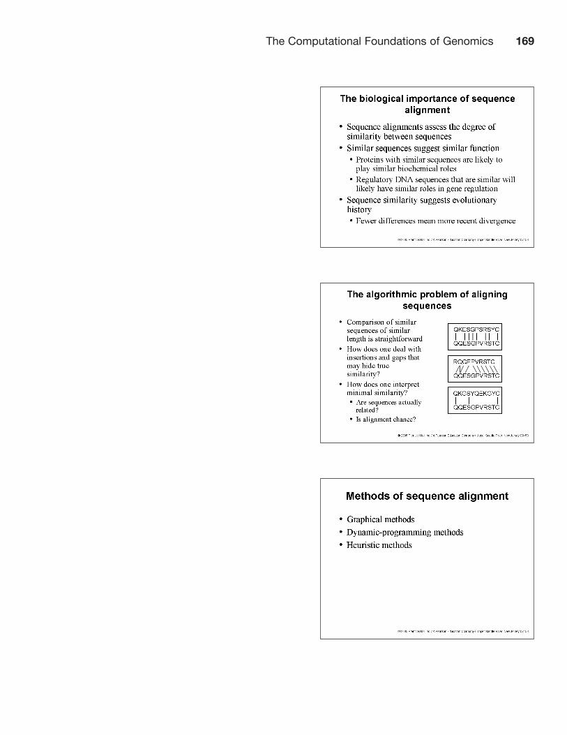
Sequence alignments allow biologists to quantify the de-gree of similarity between sequences. Similar sequencesare likely to have similar functions. For example, pro-teins with similar amino acid sequences are likely tohave biochemical roles that are related. Likewise, simi-lar DNA sequences in the regulatory regions of genesindicate that such genes are likely to be regulated by thesame transcription factors. Sequence similarities also in-dicate evolutionary relationships, with fewer differencesbetween the genes indicating a more recent common an-cestral gene. A number of terms have been developed todescribe sequences that are related (i.e., similar) to eachother. Sequences in different organisms are said to be or-thologs when they can be traced to a common ancestor.

The comparison of two closely related sequences of near-ly identical length is straightforward and can usually beachieved through visual inspection. This ease of compar-ison is obvious from the top sequence comparison in theslide. Sequence alignment becomes a more difficult algo-rithmic problem when one has to consider the effects ofinsertions and deletions. In the second sequence compar-ison in the slide, the addition of one amino acid and thedeletion of another show that only a single amino acidmatches in the alignment; yet, the red lines show thatmost of the amino acids in the two sequences are in anidentical order. More algorithmic difficulties arise whenwe consider alignments between sequences that do notappear to be closely related. How does one determinewhether these sequences are actually related? It may be

possible that the alignment has occurred by chance anddoes not indicate a significant biological relationship.

Algorithms dealing with the complexities of sequencealignment can be grouped into three categories: graphicalmethods, dynamic–programming methods, and heuristicmethods. Graphical approaches provide ways for humansto visually assess the type and quality of sequence align-ments. Dynamic programming methods can be mathe-matically proven to provide the best possible sequencealignment, but often require too much computer process-ing. Practical considerations have therefore led to the de-velopment of heuristic algorithms that usually (but notalways) provide optimal results and execute much fasterthan dynamic-programming methods.


The figures in this slide show real-world examples of dotmatrix analyses. Window size refers to the chunks of se-quence that will be compared at a time. Stringency setsthe minimum number of amino acid or nucleotide match-es in each window that is necessary for match to berecorded in the dot matrix analysis. In the slide, two se-quences that are approximately 800 nucleotides long areinitially compared with a window size of 1 and a strin-gency of 1. This comparison results in a mess that cannotbe interpreted; however, when the window size is set to23 and the stringency to 15, a very clear alignment be-comes apparent in the lower right quadrant of the matrix.

The remaining methods for sequence alignment requirescoring methods to quantify the quality of sequence align-ments. This analysis is necessary if one is searching forthe best possible alignment. To fulfill this function, compu-tational biologists have developed scoring matrices that aregenerated using statistics from real nucleotide and aminoacid sequences. Different scoring matrices are used fordifferent purposes. For example, PAM (Percent AcceptedMutation) scoring matrices are used in evolutionary studies,and BLOSUM (BLOcks amino acid SUbstitution Matrix)scoring matrices are used when looking for common func-tional motifs in proteins. The next slide shows an exampleof how a scoring matrix works.

170 Chapter 6

Dot matrix analysis is a graphical method that displays allpossible alignments between two nucleotide or protein se-quences. Gaps and insertions do not affect the perform-ance of this method. The example in the slide uses asequence comparison from the previous slide. The redboxes in the matrix on the slide show amino acid matchesbetween the two sequences. The long string of red boxesshows that the two sequences are definitely related. Theyellow diagonal on the matrix indicates boxes that wouldhave been red had the first 10 amino acids of the two se-quences been identical. When a diagonal of red boxes isdisplaced from the yellow line, the presence of insertions(or deletions) is indicated. Compared with other sequencealignment methods, dot matrix analysis is less rigorous

and requires some guesswork on the part of users to pickparameters such as window size and stringency.


172 Chapter 6

of subsequence comparisons that is necessary to findthe optimal alignment for the two sequences in ques-tion. DP algorithms are for two sequences thathave N amino acids or nucleotides. These methods arealso mathematically proven to provide the optimalalignment between two sequences for a given scoringmatrix. DP algorithms for sequence alignment includethe Needleman–Wunsch–Gotoh algorithm for globalalignments and the Smith–Waterman algorithm for localalignments. Unfortunately, DP algorithms often lack thespeed necessary to perform sequence alignments overentire sequence databases. In most cases, biologists areforced to use heuristic methods for such tasks.

O1N22

K-tuple methods are heuristic sequence-alignment algo-rithms that are much faster than dynamic programmingand usually provide optimal alignments, though not prov-ably so. These methods are excellent for comparing aquery sequence with an entire sequence database. Twopopular k-tuple programs are BLAST (Basic LocalAlignment Search Tool) and FASTA. We use the BLASTprogram to illustrate how k-tuple algorithms work. Thequery sequence is used to derive a list of “words” (or “tu-ples”) that are of a length specified by the user. For ex-ample, the sequence ABCDE can be divided into threewords with three letters each: ABC, BCD, and CDE. Thisstep is shown in part A of the figure in the slide. Eachword is then scored (using a scoring matrix) against data-base sequences, and the highest scoring words are re-tained and used for subsequent searches. Sequences in

The matrix on the right side of the slide is a subset of thefull BLOSUM62 scoring matrix. A sample sequencecomparison is shown on the left. Green signifies a scoreof zero. Red and blue signify positive and negative scores,respectively. Note that positive scores tend to representconservative amino acid changes.

The possibility of gaps (or insertions) makes the numberof possible sequence alignments between two sequencesastronomical; therefore, the problem of sequence align-ment requires powerful computational methods for its so-lution. Dynamic programming (DP) is an approach usedto solve a wide variety of problems in computer science.Its power comes from its ability to break up a large prob-lem into many smaller subproblems that are then solvedto achieve a solution to the larger problem. In the case ofsequence alignment, two sequences are broken up intoever smaller subsequences, until only single amino acidsor nucleotides are being compared. Each comparison isscored, and low-scoring subsequences are removed fromany additional processing, greatly decreasing the number

the database that have many exact matches to high-scoringwords are selected for further processing (shown in partB). Finally, the high-scoring words are used as anchors toguide the sequence alignment between the query sequenceand a high-scoring sequence returned from the database.The two sequences are shifted over each other to maximizethe alignment score.


174 Chapter 6

Even when a sequence alignment is found, biologists needa way to determine whether it is likely to be biologicallysignificant. Chance alignments do not reveal any kind ofbiological relationship. It is possible that some sequencesimilarities arise by chance and do not indicate a commonancestry between two sequences. A short strand of DNAlike AGCT illustrates this point. The probability of anoth-er four-base-pair sequence having the same composition is

or This may seem like a low-proba-bility event, but if the sequences we are comparing withAGCT have hundreds or thousands of base pairs, then wewould expect that a great number of sequences will con-tain this pattern. Given the high probability that this patternwill arise by chance, it would be unwise to assume that allof these sequences are somehow biologically related. Ofcourse, the possibility always exists, even for almost iden-tical sequences, that the sequences arose independentlyand are not biologically related. Therefore, probabilitythresholds (i.e., thresholds for statistical significance) mustbe set by biologists who wish to say that two sequences arelikely to be related. For example, a biologist may wish toconsider all sequences that have less than a 1/1,000 proba-bility of aligning by chance to be biologically related.Calculating the likelihood of a chance alignment exactly ismore complicated than the simple example we looked atpreviously. It requires taking two aligned sequences, re-peatedly scrambling one, calculating the alignment scorewith the scrambled sequence, generating a histogram fromthis process (occurrence vs. score), and then calculatingthe probability of the optimal alignment occurring by

1256.1

4 * 14 * 1

4 * 14,

The BLAST homepage (http://www.ncbi.nlm.nih.gov/BLAST/) can be found on the National Center forBiotechnology Information (NCBI) website. Sequencealignments are performed free of charge and cover allavailable public sequence databases. The slide shows thetop of the query page for protein–protein BLAST, a pro-gram that performs sequence alignments on amino acidsequences. A query sequence is entered in the “Search”text box. For the purpose of this example, we have cho-sen MASH-1, a transcription factor that regulates neuraldevelopment in rats. By clicking on the “BLAST!” but-ton, the user submits the query sequence for alignment.Because the amount of time to perform a sequence align-ment can vary greatly, the BLAST program gives the useran estimate for the time it will take to return the results.The results for the MASH-1 query are shown in the nextslide.

chance. The distribution of chance-alignment scores is de-scribed by a curve called the extreme-value distribution.This curve is used to generate probabilities for the deter-mination of statistical significance.


176 Chapter 6

The graphical display in the slide shows the sequencesthat BLAST was able to align to the MASH-1 amino acidsequence. Alignment scores are represented on the colorbar at the top of the figure, with scores going from low(black) to high (red). The numbered line below the colorbar represents the amino acid sequence of MASH-1.Below it are various sequences from several databasesthat were found to align to MASH-1. The precise posi-tion of each sequence relative to the MASH-1 sequenceindicates the areas of sequence similarity. The next slideshows the BLAST results in greater detail.

This slide shows a list of significant sequence alignmentsto MASH-1. Alignments were scored using the BLO-SUM62 scoring matrix discussed previously. The E val-ues, shown on the far right, measure the probability offinding a particular alignment by chance in the databasebeing searched. As the E values approach zero, the statis-tical significance of the alignment increases. Note howsmall the E values are for the most significant alignments.

One of the significant alignments to MASH-1 was aprotein called HASH-2, a human homolog of MASH-1.The bottom of the slide shows a pairwise alignment ofthese two sequences that was generated by BLAST. The“Query” sequence refers to MASH-1 and the “Sbjct” se-quence to HASH-2. Amino acids that are identical in thealignment are shown in the row of characters between thetwo sequences. Plus signs in this row indicate conserva-tive amino acid substitutions. The minus signs in theoriginal sequences represent deletions (or insertions).The X’s in the MASH-1 sequence are not amino acids,but instead indicate an area of low complexity. Theseareas typically contain short repeats and can create prob-lems in sequence alignments because they generate highscores that do not actually reflect the biological rela-tionship of the two sequences. An example of a low-complexity area would be the amino acid sequence

PPCDPPPPPKDKKKKDDGPP. The BLAST programand the NCBI website are constantly being enhanced.The reader is urged to go to the website and experimentwith his or her favorite sequences.


178 Chapter 6

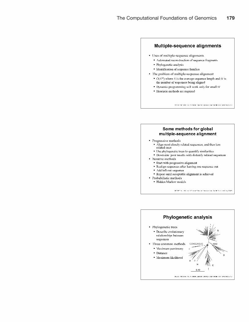
So far, we have discussed pairwise sequence alignments.Alignments that involve more than two sequences arereferred to as multiple-sequence alignments. Multiple-sequence alignments are necessary for phylogeneticanalyses, the identification of sequence families, and theautomated reconstruction of gene fragments in sequenc-ing projects. Unfortunately, methods for finding optimalalignments (i.e., dynamic programming methods) amongmultiple sequences are only practical for 8–10 sequences.This is because optimal methods are where N isthe average length of the sequences and M is the numberof sequences. Therefore, in almost every case heuristicmethods are necessary.

Heuristic methods for multiple-sequence alignments canbe divided into progressive, iterative, and probabilisticmethods. Progressive methods align the most closely re-lated sequences first and then less related sequences.These techniques do not work well for distantly relatedsequences. Iterative methods often start with a progres-sive alignment, remove a sequence from an alignment,and then use the remaining sequences to build a “profile”of the alignment. The profile is then used to realign thesequence that had been removed. The process is then re-peated until an acceptable alignment has been achieved.There are also probabilistic methods for global sequencealignments that use hidden Markov models, described ingreater detail later in this chapter.

The figure in the slide shows a phylogenetic tree describ-ing the relationship of human immunodeficiency virusesfrom around the world. Understanding phylogeny is cen-tral to understanding biology because phylogeny revealsthe evolutionary relationships of organisms (or at leastsequences) to one another. Three methods for buildingphylogenetic trees are commonly used: maximum parsi-mony, distance, and maximum likelihood.

O1NM2,


180 Chapter 6

Once a group of sequences is aligned, the maximum-parsimony method constructs a tree for each base-pair(or amino acid) column in the aligned sequences. Severaltrees are possible, but only the ones that minimize the totalnumber of base-pair changes are retained. This process isrepeated for every base-pair position, and each of the treesgenerated is then used to construct a larger tree that takesthe full diversity of the sequences into consideration.Maximum parsimony is guaranteed to produce an optimaltree under these conditions. The maximum-likelihoodmethod aims to find the most probable tree given a set ofevolutionary assumptions (e.g., a scoring system for base-pair substitutions). It is similar to maximum parsimony inthat it constructs a tree for each column in the alignmentand that one might expect the tree requiring the least num-ber of base-pair changes to be the most probable tree

in general; however, one of the big advantages of themaximum-likelihood method is that it allows researchersto apply different evolutionary models to different sub-sets of sequences being used in the phylogenetic analysis.This feature is especially useful when sequences are dis-tantly related. In such cases, maximum parsimony doesnot work as well as maximum likelihood. Distance meth-ods search for pairs of sequences that have the least num-ber of base-pair differences and group them together asneighbors on a phylogenetic tree. In general, maximumparsimony can be used for closely related sequences, dis-tance is good for less well related sequences, and maxi-mum likelihood is useful for sequences that are distantlyrelated. Researchers often use multiple methods in orderto increase confidence in their results.

There are usually four steps in phylogenetic analysis:multiple-sequence alignment, creation of a substitutionmodel (or scoring matrix), tree building, and tree evalua-tion. Like multiple-sequence alignment, tree building andtree evaluation are often computationally expensive stepsthat require heuristic methods for all phylogenetic analy-ses that involve more than 8–10 sequences.

Gene prediction algorithms attempt to determine whethera particular DNA sequence constitutes a working gene.The parameters distinguishing genes from nongenes arenot well understood. Although certain features, such assplice sites and ORFs, are fairly well defined, other fea-tures, such as regulatory regions, are still very difficult topredict. Even identifying ORFs is not straightforward,particularly in mammalian genomes that are character-ized by small exons and large introns. A further problemin gene prediction is that our knowledge of identifyingfeatures in genes is constantly expanding. Computer sci-entists would classify gene prediction as a problem inpattern recognition. Machine learning algorithms aregood for solving problems in pattern recognition becausethey can be trained on a sample data set to “learn” whatdefines the pattern in question when well-defined rulesare not available.


sufficient input from other units. The strength of the con-nections between units changes during training andthis is what allows the network to ‘learn’ a pattern. Afully trained network can then recognize the training pat-tern in a novel input. An example of a gene predictionprogram that uses neural networks is GrailEXP.

1wij2

182 Chapter 6

Artificial neural networks are a class of machine learningalgorithms that mimic the behavior of networks of realneurons in the brain. A typical artificial neural networkbegins with an input layer, where patterns are presentedto the network for training or recognition. The slideshows an example of a feed-forward neural network, socalled because connections go in only one direction.Units in the input layer are marked by the Greek letter . Following the input layer may be one or more hiddenlayers, followed finally by an output layer that indicateswhat kind of pattern has been recognized. In the slide, thehidden units are marked with the letter V and output unitswith the letter O. Units in the input, hidden, and outputlayers are connected in various ways depending on thetype of neural network. A unit will activate, if there is

j

A Markov process is a process in which a future state de-pends on the present state, but not on past states. Markovprocesses describe many biological phenomena, includ-ing base-pair substitutions resulting from mutations. Insome cases, the states in a Markov process are not knownwith certainty. The example of a dishonest gambler isoften used to illustrate this point. The gambler may carrya loaded die that he or she occasionally substitutes for afair die, but not so often that the other players would no-tice. The fair die has a one-in-six chance of showing anyparticular number. When using the loaded die, a playerwill have a 50% chance of rolling a one and a 10%chance of rolling any other number. It is in these types ofsituations that stochastic models called hidden Markovmodels (HMMs) are useful, because they take into ac-count unknown (or hidden) states. For example, exactlywhen the cheating gambler is using a fair or loaded die ishidden from the other players, but insight may still begained by looking at the outcome of the cheater’s rolls. Ifhe or she rolls three ones in a row, it is more likely (a12.5% chance) that the loaded die is being used than thefair one, which would have only a 0.5% chance of gener-ating three ones in a row. Hidden Markov models de-scribe the probability of transitions between hiddenstates, as well as the probabilities associated with eachstate. In the example of the cheating gambler, an HMMwould describe the probabilities of rolling particularnumbers given the loaded or fair die and the probabilitythat the dishonest gambler would switch from one die to

another. Hidden Markov models can be used to answerthree types of questions. The first type is the likelihoodquestion: Given a particular HMM, what is the probabil-ity of obtaining a particular outcome (e.g., rolling threeones)? The second type is the decoding question: Givena particular HMM, what is the most likely sequence oftransitions between states for a particular outcome? In thecase of the cheating gambler, this sequence would be theorder in which he or she transitioned from one die to an-other. The third type is the learning question: Given aparticular outcome and set of assumptions about possibletransition states, what are the best model parameters(e.g., probabilities between transition states)? This thirdquestion allows HMMs to be used for machine learning.The figure in the slide shows a simple example of a hid-den Markov model being used to account for the DNAsequence at the bottom. Every HMM has a start and endstate, denoted by the S and E, respectively, in the slide.Hidden states lie between the start and end states. In thefigure, the squares are states, and the lines between themindicate the probability of one state transitioning to an-other. The loops on the upper and lower states show theprobabilities associated with the state remaining thesame. States transition back and forth until the HMMreaches the end state. In this HMM, the top square repre-sents a state that has equal probabilities of generating A,G, C, or T. The bottom state has probabilities of 0.1, 0.1,0.1, and 0.7 of generating A, G, C, and T, respectively.


The model for using HMMs to perform gene predictionis trained on a set of known genes. The HMM in the slidewas trained on 2,000 human introns. Its circular pattern isdesigned to detect repeated patterns in DNA sequences.The bars in each square represent the probabilities thatthe state will have a particular base value. Models such asthe one in this slide can be used to assess the probabilitythat a particular sequence is a gene or belongs to a certainsequence class. An example of a popular gene predictionprogram that uses HMMs is GENSCAN.

A number of algorithms have been developed to predictthe secondary structure (e.g., alpha helices and beta-pleated sheets) of proteins, based on their amino acid se-quence. One method, the Chou–Fasman / GOR method,uses experimentally determined amino acid frequenciesassociated with different kinds of secondary structures. Ifa query amino acid sequence has an amino acid compo-sition similar to that found in an experimentally deter-mined structure, it is deemed to give rise to the samesecondary structure. Other methods use machine learningalgorithms that are trained on the amino acid sequencesof secondary structures from proteins whose three-di-mensional structures have already been determined ex-perimentally. The machine learning algorithms include

184 Chapter 6

neural networks and nearest-neighbor methods. Nearest-neighbor methods look for the closest matches betweenthe query sequence and members of the training set.

Up to this point, this chapter has dealt with experimentaldata (i.e., nucleotide and amino acid sequences) that havealready been processed and archived. In this section, wefocus on bioinformatics algorithms for processing rawexperimental data generated by microarrays. Because mi-croarrays measure the expression levels of thousands ofgenes simultaneously, the data are impossible to processwithout the use of computers. Several types of analysisare possible. Analyzing the data by looking at the ex-pression levels of individual genes requires straightfor-ward statistical techniques that are used in a wide varietyof other biological experiments. Clustering algorithmsoffer a higher level of analysis that examines microarraydata in terms of groups of genes rather than single genes.Lastly, biologists would like to interpret microarray datain terms of patterns of gene regulation. Methods relatingto this avenue of research are still under development.


Algorithms used to analyze the behavior of multiple genesfall into two broad categories: supervised and unsupervised.The decision to use one or the other depends on the natureof the scientific question. For example, a biologist may havelittle intuition about what patterns of gene expression wouldappear in a sample of breast cancer tissue. An unsupervisedclustering algorithm would allow him or her to group dif-ferent sets of genes on the basis of only their gene expres-sion. An unsupervised method might uncover severalclusters of genes on the basis of how correlated their levelsof gene expression are in different tissue samples frombreast cancer patients. Armed with these results, a researchermay then wonder if a particular pattern of gene expressioncan be used in the diagnosis or prognosis of the disease. Todetermine if this can be done, supervised techniques arenecessary. These techniques assume that the microarray data

contains sufficient information to differentiate between sam-ple conditions. Supervised techniques therefore aim to findthe optimal patterns of gene expression that indicate a par-ticular sample condition. For instance, using patterns ofgene expression to differentiate between various types ofcancerous tissue can lead to a diagnosis of a specific form ofcancer that might otherwise be difficult to distinguish usingtraditional techniques. Similarly, sample tissues derivedfrom cancer patients with varying levels of mortality can beused to develop a gene expression signature indicative ofgood or poor prognosis. Examples of these types of mi-croarray applications are given in the “Pharmacogenomics”and “Genomics and Medicine” chapters. However, beforesupervised or unsupervised techniques can be used, meth-ods are needed to measure differences in gene expressionbetween individual genes.

186 Chapter 6

Several measures (metrics) are available for distinguish-ing genes on the basis of their levels of gene expression.Two of these are shown in the slide. Measuring Euclideandistance begins with a graph where the axes represent lev-els of expression in different samples. Although humanscan only visualize three dimensions, the distance betweentwo genes representing points on the graph can be meas-ured for any number of samples. The Euclidean distancebetween two genes that are expressed in two tissue sam-ples is represented by the red line in the slide. Anotherpopular measure is the Pearson correlation coefficient. Inthis case the axes are the levels of gene expression for twodifferent genes and the points on the graph represent indi-vidual tissue samples. A linear regression line is drawnthrough the points and the distance between individual

points and the line are used to calculate the Pearson cor-relation coefficient, which can take any value between and The magnitude of the coefficient represents thestrength of the relationship between two genes and thesign indicates whether the two genes are negatively orpositively correlated. For example, genes that are nega-tively correlated in their levels of gene expression wouldshow a pattern where increased expression in one gene ismarked by decreased expression in the other. While manymetrics for gene expression exist, there are caveats asso-ciated with each. For example, calculation of the Pearsoncorrelation coefficient can be compromised by the pres-ence of outliers. Nonetheless, a great deal of insight hasbeen gained by applying gene expression metrics to unsu-pervised and supervised methods.

+1.-1

Supervised techniques are used to divide groups of genesbased on already characterized differences between sam-ples (e.g., different types of malignancies) or to predictthe condition of a sample on the basis of gene expressionpatterns. The support vector machine works by searchingfor mathematical combinations of genes to best separatetissues on the basis of their condition. For example, theschematic in the top half of the slide shows how a linewas generated to separate tissue samples coming frompatients suffering from two different diseases. The x-axisrepresents the multiplication of the gene expression lev-els of two different genes, which is then squared. The y-axis uses the same mathematical expression but for adifferent set of genes. Unfortunately, the mathematicalexpressions are not always easy to understand from a bi-ological perspective. The nearest neighbor supervised

method is also schematized in the slide. A group of hy-pothetical genes is constructed to distinguish betweentwo sample states, disease 1 and disease 2. An ideal geneto separate the two disease states might be one that is up-regulated in disease 1 and down-regulated in disease 2.Real genes that fit this pattern can then be selected ashallmarks of the disease state. The nearest neighbormethod has been successfully used to distinguish be-tween two types of human leukemia.


.

188 Chapter 6

Many biologists wonder why simulations are necessarywhen an experiment can more conclusively answer a sci-entific question. One reason is that biological systems arecomplex, and it is often difficult to conceptualize a modelthat explains an experimental behavior without doing asimulation which can prove that the model is, at the veryleast, logically viable. A good simulation can then beused to devise new ways of experimentally testing a par-ticular hypothesis. Simulations have the added benefitthat, if they replicate the behavior of a biological systemwell, they can be used in place of time-consuming, ex-pensive, or impossible experiments. To illustrate this lastpoint, consider the U.S. military’s recent abandonment ofnuclear weapons testing. Until 1992, the United States

routinely conducted underground nuclear tests. Sincethen, the Pentagon has placed its faith in computer simu-lations that are considered accurate enough to make nu-clear testing obsolete!

For the last 350 years, scientists have been using differ-ential equations to describe how things change continu-ously over time in nature. Unfortunately, because digitalcomputers can represent only discrete quantities, they arenot able to deal directly with differential equations. Themathematical techniques for using discrete quantities toapproximate the behavior of differential equations arecalled numerical methods. The accuracy of numericalmethods depends on the number of calculations per-formed over an interval. An illustrative example is thegrowth of bacteria in medium. One could use numericalmethods to approximate the number of bacteria in thebroth at different times. In one case, the number of bac-teria in the broth is calculated for every 10 millisecondsof simulated time. In another case, the calculations are

done for every millisecond of simulated time. The secondcase will yield more accurate results, but will require amuch longer time to fully execute. Depending on thecomputational complexity of the numerical method, thesimulation with the 1-millisecond resolution may takehundreds or thousands of times as long to run as the onewith the 10-millisecond resolution.

Computer simulations of biological systems have existedfor decades, though early simulations had to forsake bio-logical detail because of the insufficient processingpower of early computers. Biological simulations coverthe entire range of scale in the biological world, from in-dividual protein molecules to population genetics. Otherimportant areas of computer simulation include gene reg-ulatory networks, biochemical pathways, single cells,and networks of neurons to simulate activity in the brain.The slide shows an example of a simulation of gene reg-ulation in a bacterial virus. The top part of the imageshows the complexity of gene regulation. The bottompart shows output from the simulation, showing differentlevels of repressor protein.


Large-scale biology projects for understanding genomes,proteomes, metabalomes, and transcriptomes have ledmany biologists to conclude that the possibility of a fullysimulated single cell is not as unlikely a prospect as pre-viously thought. Since the late 1990s, a number of sim-plified models of single cells have been constructed, withvarying degrees of success. More recently, a group inJapan has been simulating human erythrocytes (red bloodcells). These cells are especially amenable to simulationbecause they lack the cellular machinery needed for tran-scription, translation, and replication, thereby greatlyreducing the number of parameters that must be includ-ed in a realistic simulation. In addition, because of theirmedical relevance, erythrocytes have been extensively

190 Chapter 6

studied in the past 50 years, yielding a large body of re-liable data about these cells. The Japanese group hasused its virtual erythrocyte to successfully simulate thebehavior of blood cells in anemic patients. The picture inthe slide shows the various biochemical pathways that aremodeled in the in silico erythrocyte. Despite the relativesimplicity of the human blood cell, the picture indicatesthat the simulation is still quite complex. Though themodel cell continues to be refined for accuracy, it is animportant proof of concept for the usefulness of simula-tions in the medical realm. The hope is that simulatedcells will someday be used to test new drugs and to studythe effects of mutant proteins responsible for disease.

Despite their usefulness, computer simulations have a va-riety of caveats. At the algorithmic level, the inability ofcomputers to manipulate continuous quantities requiresthat the computers approximate continuous behaviorwith ever smaller steps that greatly increase the require-ments for processing power and memory. Although sys-tems that do not change dramatically over small distancesor over short periods of time can be simulated with suffi-cient accuracy, many important biological phenomena,such as protein folding, do not fit this criterion andhave not yielded realistic simulation results to date.Experimental considerations also plague many simula-tions. For example, simulations require high-quality data,which are not always available. Often, researchers must

speculate about the values of parameters in their simula-tion. Other times, simulations may reveal that a previouslyignored parameter is absolutely necessary for the simula-tion to behave correctly. A serious conceptual issue ariseswhen simulations become too complex. A simulation thatis as complex as the biological system it attempts tomodel has little explanatory power. By analogy, considera map of the United States that is so detailed that it con-tains even the most miniscule element of the terrain. Onemight expect such a map to be the size of the country it-self and thus hardly useful when traveling.

In this chapter, we have seen that the vast amounts of datagenerated by genomics projects require computationalapproaches. The ability to apply bioinformatics methodsis limited by the algorithmic complexity of the computa-tional problem and the performance of the available com-puter hardware. To address situations that are beyondcurrent capabilities, heuristic methods can be used. Wehave discussed the applications of bioinformatics meth-ods to sequence alignment, phylogenetic-tree construc-tion, gene prediction, secondary-structure determination,the analysis of microarray data, and the simulation of bi-ological systems.


Documents

Chapter 6 The Computational Foundations of Genomicsesminfo.prenhall.com/.../benfeyinfo/closerlook/pdf/samplechapter.pdf · This chapter describes the computational methods that have