Chapter 6: Production 1 of 24 Copyright © 2009 Pearson Education, Inc. Publishing as Prentice Hall Microeconomics Pindyck/Rubinfeld, 7e. PRODUCTION

Ch

apte

r 6:

P

rod

uct

ion

1 of 24Copyright © 2009 Pearson Education, Inc. Publishing as Prentice Hall • Microeconomics • Pindyck/Rubinfeld, 7e.

PRODUCTION

Ch

apte

r 6:

P

rod

uct

ion


CHAPTER OUTLINE

6.1 The Technology of Production

6.2 Production with One Variable Input (Labor)

6.3 Production with Two Variable Inputs

6.4 Returns to Scale

Ch

apte

r 6:

P

rod

uct

ion


Production

The theory of the firm describes how a firm makes cost-minimizing production decisions and how the firm’s resulting cost varies with its output.

The production decisions of firms are analogous to the purchasing decisions of consumers, and can likewise be understood in three steps:

1. Production Technology

2. Cost Constraints

3. Input Choices

The Production Decisions of a Firm

Ch

apte

r 6:

P

rod

uct

ion


THE TECHNOLOGY OF PRODUCTION6.1

The Production Function

● factors of production Inputs into the production process (e.g., labor, capital, and materials).

Remember the following:

( , ) (6.1)q F K L

Inputs and outputs are flows.

Equation (6.1) applies to a given technology

Production functions describe what is technically feasible when the firm operates efficiently.

●production function Function showing the highest output that a firm can produce for every specified combination of inputs.

Ch

apte

r 6:

P

rod

uct

ion


THE TECHNOLOGY OF PRODUCTION6.1

The Short Run versus the Long Run

●short run Period of time in which quantities of one or more production factors cannot be changed.

● fixed input Production factor that cannot be varied.

● long run Amount of time needed to make all production inputs variable.

Ch

apte

r 6:

P

rod

uct

ion


TABLE 6.1 Production with One Variable Input

0 10 0 — —

1 10 10 10 10

2 10 30 15 20

3 10 60 20 30

4 10 80 20 20

5 10 95 19 15

6 10 108 18 13

7 10 112 16 4

8 10 112 14 0

9 10 108 12 4

10 10 100 10 8

PRODUCTION WITH ONE VARIABLE INPUT (LABOR)6.2

TotalOutput (q)

Amountof Labor (L)

Amountof Capital (K)

AverageProduct (q/L)

MarginalProduct (∆q/∆L)

Ch

apte

r 6:

P

rod

uct

ion



Average and Marginal Products

● average product Output per unit of a particular input.

● marginal product Additional output produced as an input is increased by one unit.

Average product of labor = Output/labor input = q/L

Marginal product of labor = Change in output/change in labor input = Δq/ΔL

Ch

apte

r 6:

P

rod

uct

ion



The Slopes of the Product Curve

The total product curve in (a) shows the output produced for different amounts of labor input.

The average and marginal products in (b) can be obtained (using the data in Table 6.1) from the total product curve.

At point A in (a), the marginal product is 20 because the tangent to the total product curve has a slope of 20.

At point B in (a) the average product of labor is 20, which is the slope of the line from the origin to B.

The average product of labor at point C in (a) is given by the slope of the line 0C.

Production with One Variable Input

Figure 6.1

Ch

apte

r 6:

P

rod

uct

ion



The Slopes of the Product Curve

To the left of point E in (b), the marginal product is above the average product and the average is increasing; to the right of E, the marginal product is below the average product and the average is decreasing.

As a result, E represents the point at which the average and marginal products are equal, when the average product reaches its maximum.

At D, when total output is maximized, the slope of the tangent to the total product curve is 0, as is the marginal product.

Production with One Variable Input

(continued)

Figure 6.1

Ch

apte

r 6:

P

rod

uct

ion



The Law of Diminishing Marginal Returns

Labor productivity (output per unit of labor) can increase if there are improvements in technology, even though any given production process exhibits diminishing returns to labor.

As we move from point A on curve O1 to B on curve O2 to C on curve O3 over time, labor productivity increases.

The Effect of Technological Improvement

Figure 6.2

● law of diminishing marginal returns Principle that as the use of an input increases with other inputs fixed, the resulting additions to output will eventually decrease.

Ch

apte

r 6:

P

rod

uct

ion


Productivity and the Standard of Living

●stock of capital Total amount of capital available for use in production.

● technological change Development of new technologies allowing factors of production to be used more effectively.

Labor Productivity


● labor productivity Average product of labor for an entire industry or for the economy as a whole.

Ch

apte

r 6:

P

rod

uct

ion


LABOR INPUT

PRODUCTION WITH TWO VARIABLE INPUTS6.3

TABLE 6.4 Production with Two Variable Inputs

Capital Input

1 2 3 4 5

1 20 40 55 65 75

2 40 60 75 85 90

3 55 75 90 100 105

4 65 85 100 110 115

5 75 90 105 115 120

Isoquants

● isoquant Curve showing all possible combinations of inputs that yield the same output.

Ch

apte

r 6:

P

rod

uct

ion



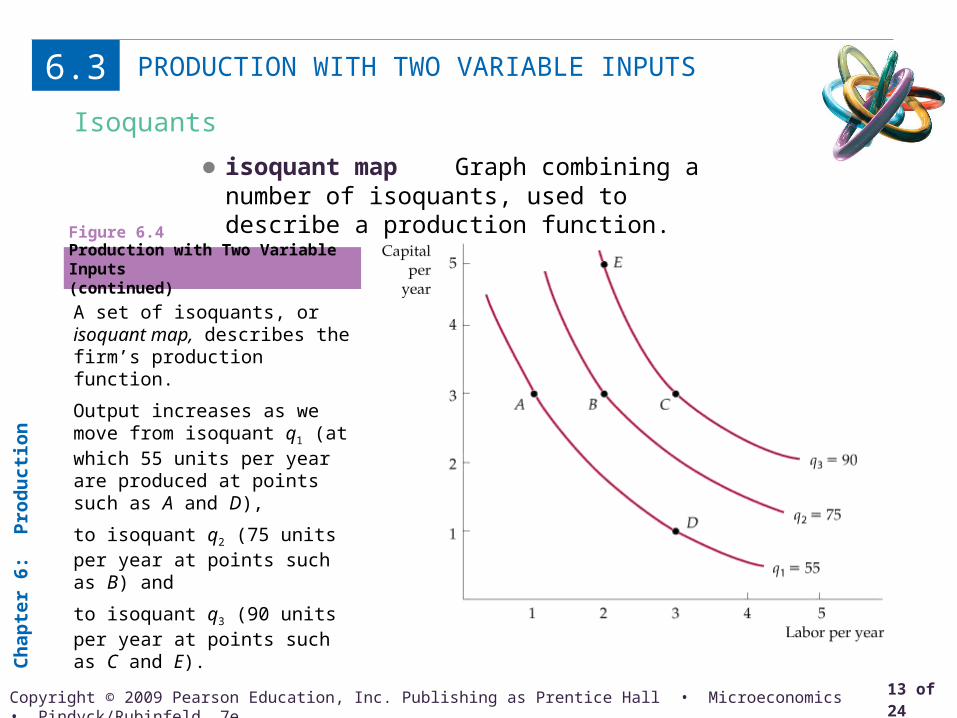
Isoquants

● isoquant map Graph combining a number of isoquants, used to describe a production function.

A set of isoquants, or isoquant map, describes the firm’s production function.

Output increases as we move from isoquant q1 (at which 55 units per year are produced at points such as A and D),

to isoquant q2 (75 units per year at points such as B) and

to isoquant q3 (90 units per year at points such as C and E).

Production with Two Variable Inputs(continued)

Figure 6.4

Ch

apte

r 6:

P

rod

uct

ion



Diminishing Marginal Returns

Diminishing Marginal Returns Holding the amount of capital fixed at a particular level—say 3, we can see that each additional unit of labor generates less and less additional output.

Production with Two Variable Inputs(continued)

Figure 6.4

Ch

apte

r 6:

P

rod

uct

ion


PRODUCTION WITH TWO VARIABLE INPUTS6.3Substitution Among Inputs

Like indifference curves, isoquants are downward sloping and convex. The slope of the isoquant at any point measures the marginal rate of technical substitution—the ability of the firm to replace capital with labor while maintaining the same level of output.

On isoquant q2, the MRTS falls from 2 to 1 to 2/3 to 1/3.

Marginal rate of technical substitution

Figure 6.5

● marginal rate of technical substitution (MRTS) Amount by which the quantity of one input can be reduced when one extra unit of another input is used, so that output remains constant.

MRTS = − Change in capital input/change in labor input

= − ΔK/ΔL (for a fixed level of q)

(MP ) / (MP ) ( / ) MRTSK LL K

Ch

apte

r 6:

P

rod

uct

ion


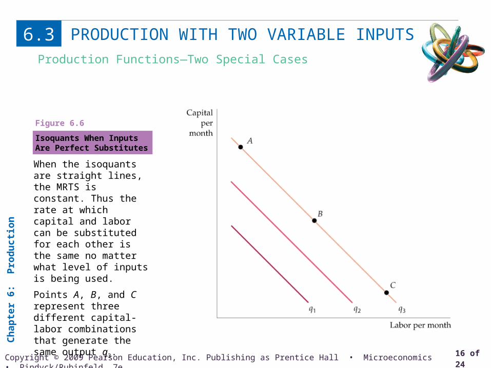
PRODUCTION WITH TWO VARIABLE INPUTS6.3Production Functions—Two Special Cases

When the isoquants are straight lines, the MRTS is constant. Thus the rate at which capital and labor can be substituted for each other is the same no matter what level of inputs is being used.

Points A, B, and C represent three different capital-labor combinations that generate the same output q3.

Isoquants When Inputs Are Perfect Substitutes

Figure 6.6

Ch

apte

r 6:

P

rod

uct

ion


PRODUCTION WITH TWO VARIABLE INPUTS6.3Production Functions—Two Special Cases

When the isoquants are L-shaped, only one combination of labor and capital can be used to produce a given output (as at point A on isoquant q1, point B on isoquant q2, and point C on isoquant q3). Adding more labor alone does not increase output, nor does adding more capital alone.

The fixed-proportions production function describes situations in which methods of production are limited.

Fixed-Proportions Production Function

Figure 6.7

● fixed-proportions production function Production function with L-shaped isoquants, so that only one combination of labor and capital can be used to produce each level of output.

Ch

apte

r 6:

P

rod

uct

ion


RETURNS TO SCALE6.4

● returns to scale Rate at which output increases as inputs are increased proportionately.

● increasing returns to scale Situation in which output more than doubles when all inputs are doubled.

● constant returns to scale Situation in which output doubles when all inputs are doubled.

● decreasing returns to scale Situation in which output less than doubles when all inputs are doubled.

Ch

apte

r 6:

P

rod

uct

ion


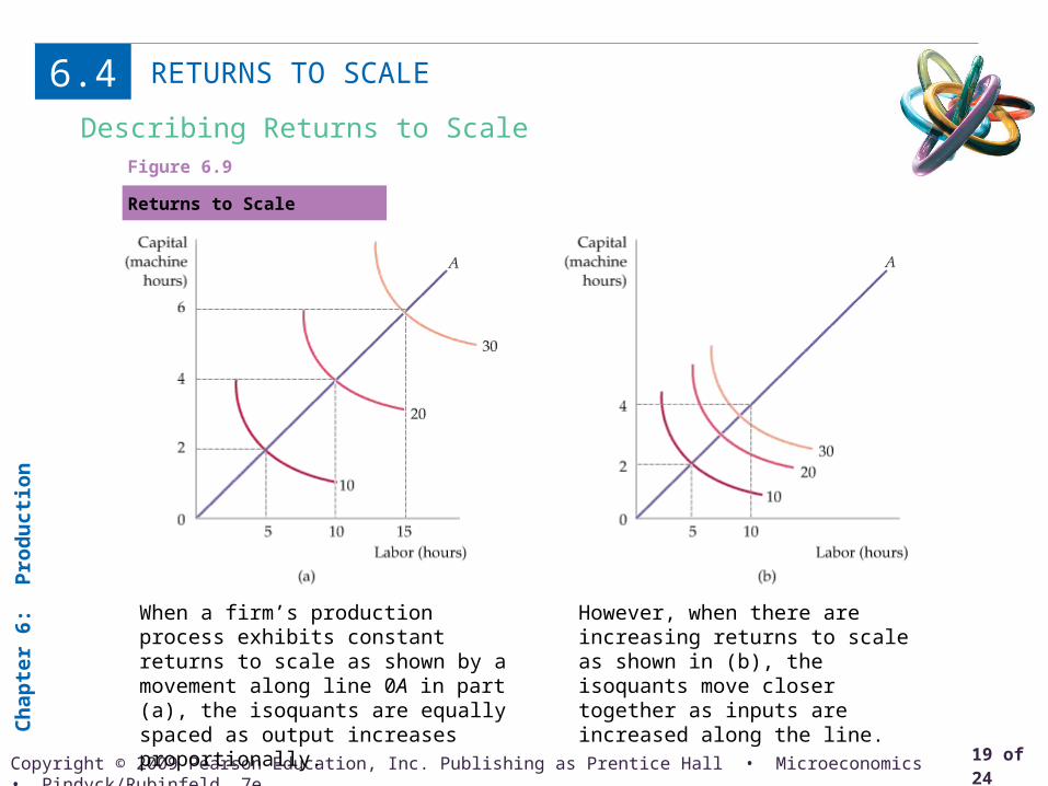
RETURNS TO SCALE6.4

When a firm’s production process exhibits constant returns to scale as shown by a movement along line 0A in part (a), the isoquants are equally spaced as output increases proportionally.

Returns to Scale

Figure 6.9

However, when there are increasing returns to scale as shown in (b), the isoquants move closer together as inputs are increased along the line.

Describing Returns to Scale

Documents

Chapter 6: Production 1 of 24 Copyright © 2009 Pearson Education, Inc. Publishing as Prentice Hall Microeconomics Pindyck/Rubinfeld, 7e. PRODUCTION