Embed Size (px)
Citation preview
Chapter 6 Production
Read Pindyck and Rubinfeld (2013), Chapter 6
•Chapter 6 Production . Chairat Aemkulwat . Economics I: 2900111 1/29/2017
CHAPTER 6 OUTLINE
6.1 The Technology of Production
6.2 Production with One Variable Input (Labor)
6.3 Production with Two Variable Inputs
6.4 Returns to Scale
•Chapter 6 Production . Chairat Aemkulwat . Economics I: 2900111
Production
• The Production Decisions of a Firm
The theory of the firm describes how a firm makes cost-
minimizing production decisions and how the firm’s
resulting cost varies with its output.
The production decisions of firms are analogous to the
purchasing decisions of consumers, and can likewise be
understood in three steps:
1. Production Technology
2. Cost Constraints
3. Input Choices
•Chapter 6 Production . Chairat Aemkulwat . Economics I: 2900111 •3
Copyright © 2009 Pearson Education, Inc. Publishing as Prentice Hall • Microeconomics • Pindyck/Rubinfeld, 7e.
Why Do Firms Exist?
• Firms and Their Production Decisions•6.1
• Firms offer a means of coordination that is extremely important and would be sorely missing if workers operated independently.
• Firms eliminate the need for every worker to negotiate every task that he or she will perform, and bargain over the fees that will be paid for those tasks.
‐ Firms can avoid this kind of bargaining by having managers that direct the production of salaried workers—they tell workers what to do and when to do it, and the workers (as well as the managers themselves) are simply paid a weekly or monthly salary.
THE TECHNOLOGY OF PRODUCTION
• The Production Function
6.1
● factors of production Inputs into the production
process (e.g., labor, capital, and materials).
Remember the following:
( , ) (6.1)q F K L
Inputs and outputs are flows.
Equation (6.1) applies to a given technology
Production functions describe what is technically feasible
when the firm operates efficiently.
● production function Function showing the highest
output that a firm can produce for every specified
combination of inputs.
•5•Chapter 6 Production . Chairat Aemkulwat . Economics I: 2900111
THE TECHNOLOGY OF PRODUCTION
• The Short Run versus the Long Run
6.1
● short run Period of time in which quantities of one or
more production factors cannot be changed.
● fixed input Production factor that cannot be varied.
● long run Amount of time needed to make all
production inputs variable.
•6•Chapter 6 Production . Chairat Aemkulwat . Economics I: 2900111
PRODUCTION WITH ONE VARIABLE INPUT (LABOR)
• Average and Marginal Products
6.2
● average product Output per unit of a particular input.
● marginal product Additional output produced as an input is
increased by one unit.
Marginal product of labor = Change in output/change in labor input
= Δq/ΔL
•7•Chapter 6 Production . Chairat Aemkulwat . Economics I: 2900111
Average product of labor = Output/labor input = q/L
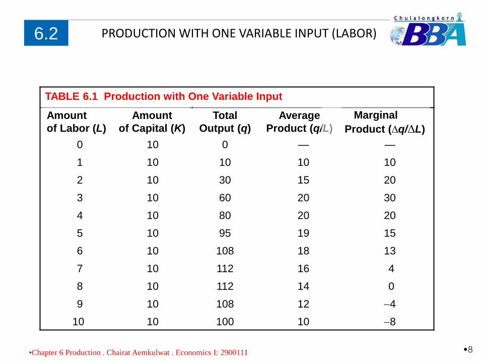
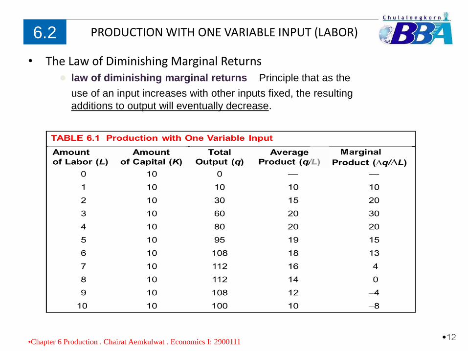
TABLE 6.1 Production with One Variable Input
0 10 0 — —
1 10 10 10 10
2 10 30 15 20
3 10 60 20 30
4 10 80 20 20
5 10 95 19 15
6 10 108 18 13
7 10 112 16 4
8 10 112 14 0
9 10 108 12 4
10 10 100 10 8
PRODUCTION WITH ONE VARIABLE INPUT (LABOR)6.2
Total
Output (q)
Amount
of Labor (L)
Amount
of Capital (K)
Average
Product (q/L)
Marginal
Product (∆q/∆L)
•8•Chapter 6 Production . Chairat Aemkulwat . Economics I: 2900111
PRODUCTION WITH ONE VARIABLE INPUT (LABOR)
• The Slopes of the Product Curve
6.2
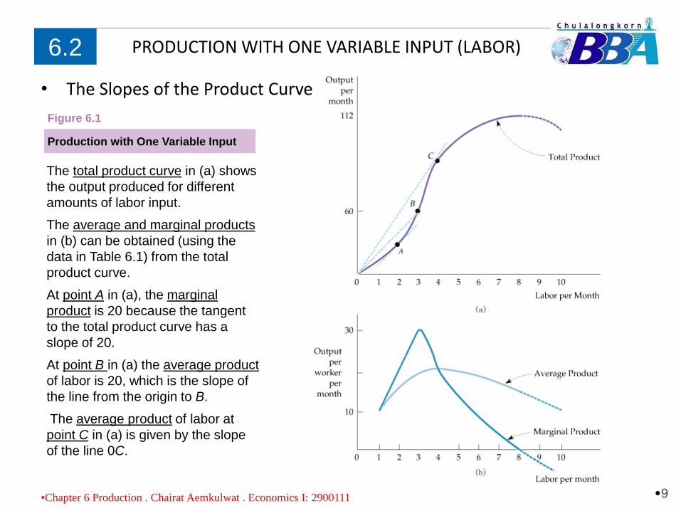
The total product curve in (a) shows
the output produced for different
amounts of labor input.
The average and marginal products
in (b) can be obtained (using the
data in Table 6.1) from the total
product curve.
At point A in (a), the marginal
product is 20 because the tangent
to the total product curve has a
slope of 20.
At point B in (a) the average product
of labor is 20, which is the slope of
the line from the origin to B.
The average product of labor at
point C in (a) is given by the slope
of the line 0C.
Production with One Variable Input
Figure 6.1
•9•Chapter 6 Production . Chairat Aemkulwat . Economics I: 2900111
PRODUCTION WITH ONE VARIABLE INPUT (LABOR)
• The Slopes of the Product Curve
6.2
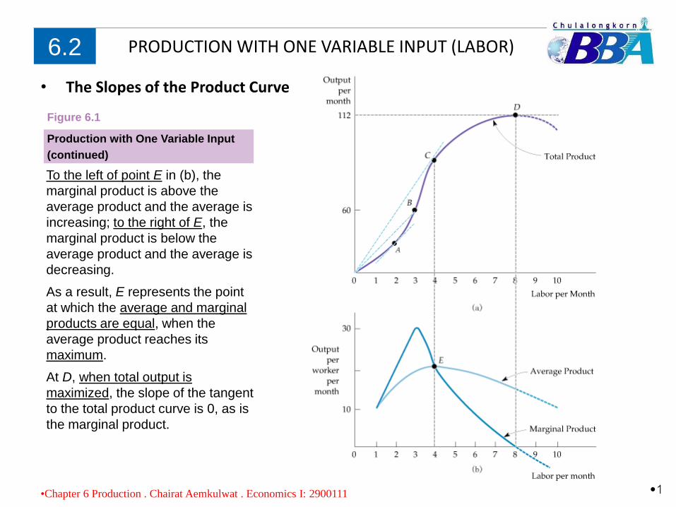
To the left of point E in (b), the
marginal product is above the
average product and the average is
increasing; to the right of E, the
marginal product is below the
average product and the average is
decreasing.
As a result, E represents the point
at which the average and marginal
products are equal, when the
average product reaches its
maximum.
At D, when total output is
maximized, the slope of the tangent
to the total product curve is 0, as is
the marginal product.
Production with One Variable Input
(continued)
Figure 6.1
•10
•Chapter 6 Production . Chairat Aemkulwat . Economics I: 2900111
Copyright © 2009 Pearson Education, Inc. Publishing as Prentice Hall • Microeconomics • Pindyck/Rubinfeld, 7e.
• The Average Product of Labor Curve
•In general, the average product of labor is given by the slope of the line drawn from the origin to the corresponding point on the total product curve.
• The Marginal Product of Labor Curve
•In general, the marginal product of labor at a point is given by the slope of the total product at that point.
• THE RELATIONSHIP BETWEEN THE AVERAGE AND MARGINAL
• PRODUCTS
•Note the graphical relationship between average and marginal products in Figure 6.1 (a). When the marginal product of labor is greater than the average product (MP>AP), the average product of labor increases.
•At C, the average and marginal products of labor are equal (MP=AP) .
•Finally, as we move beyond C toward D, the marginal product falls below the average product (MP<AP). You can check that the slope of the tangent to the total product curve at any point between C and D is lower than the slope of the line from the origin.
PRODUCTION WITH ONE VARIABLE INPUT (LABOR)
• The Law of Diminishing Marginal Returns
6.2
● law of diminishing marginal returns Principle that as the
use of an input increases with other inputs fixed, the resulting
additions to output will eventually decrease.
•12•Chapter 6 Production . Chairat Aemkulwat . Economics I: 2900111
PRODUCTION WITH ONE VARIABLE INPUT (LABOR)
• The Law of Diminishing Marginal Returns
6.2
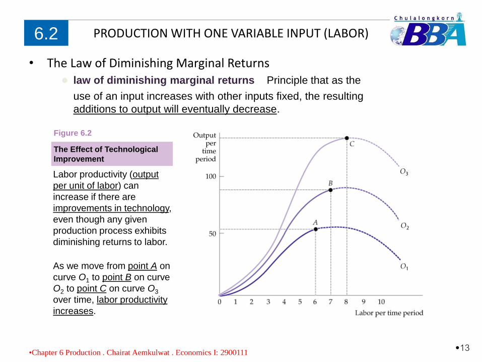
Labor productivity (output
per unit of labor) can
increase if there are
improvements in technology,
even though any given
production process exhibits
diminishing returns to labor.
The Effect of Technological
Improvement
Figure 6.2
● law of diminishing marginal returns Principle that as the
use of an input increases with other inputs fixed, the resulting
additions to output will eventually decrease.
•13•Chapter 6 Production . Chairat Aemkulwat . Economics I: 2900111
As we move from point A on
curve O1 to point B on curve
O2 to point C on curve O3
over time, labor productivity
increases.
Copyright © 2009 Pearson Education, Inc. Publishing as Prentice Hall • Microeconomics • Pindyck/Rubinfeld, 7e.
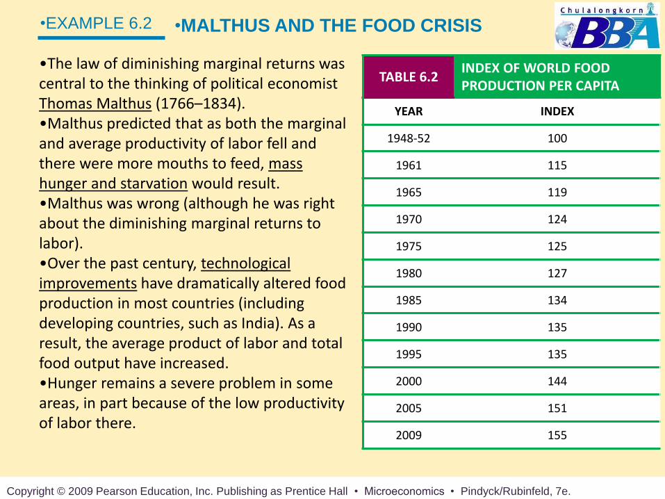
•The law of diminishing marginal returns was central to the thinking of political economist Thomas Malthus (1766–1834).•Malthus predicted that as both the marginal and average productivity of labor fell and there were more mouths to feed, mass hunger and starvation would result.•Malthus was wrong (although he was right about the diminishing marginal returns to labor).•Over the past century, technological improvements have dramatically altered food production in most countries (including developing countries, such as India). As a result, the average product of labor and total food output have increased.•Hunger remains a severe problem in some areas, in part because of the low productivity of labor there.
•EXAMPLE 6.2 •MALTHUS AND THE FOOD CRISIS
TABLE 6.2INDEX OF WORLD FOOD PRODUCTION PER CAPITA
YEAR INDEX
1948-52 100
1961 115
1965 119
1970 124
1975 125
1980 127
1985 134
1990 135
1995 135
2000 144
2005 151
2009 155
Copyright © 2009 Pearson Education, Inc. Publishing as Prentice Hall • Microeconomics • Pindyck/Rubinfeld, 7e.
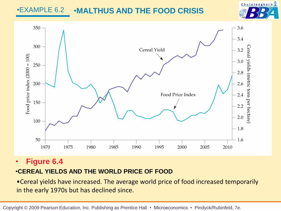
•Cereal yields have increased. The average world price of food increased temporarily in the early 1970s but has declined since.
•EXAMPLE 6.2 •MALTHUS AND THE FOOD CRISIS
•CEREAL YIELDS AND THE WORLD PRICE OF FOOD
• Figure 6.4
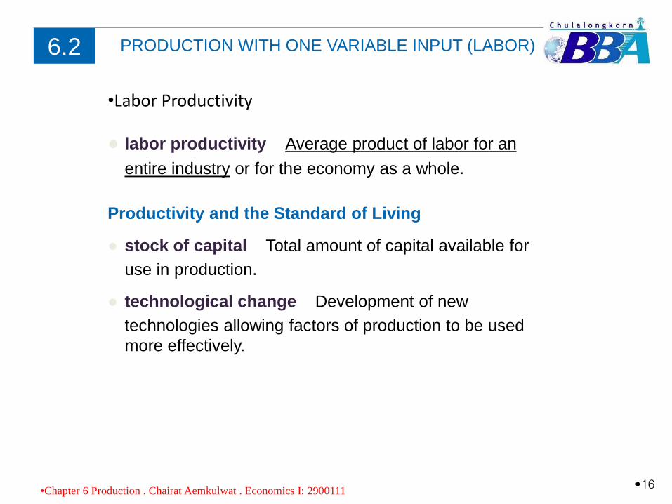
Productivity and the Standard of Living
● stock of capital Total amount of capital available for
use in production.
● technological change Development of new
technologies allowing factors of production to be used
more effectively.
•Labor Productivity
PRODUCTION WITH ONE VARIABLE INPUT (LABOR)6.2
● labor productivity Average product of labor for an
entire industry or for the economy as a whole.
•16•Chapter 6 Production . Chairat Aemkulwat . Economics I: 2900111
Copyright © 2009 Pearson Education, Inc. Publishing as Prentice Hall • Microeconomics • Pindyck/Rubinfeld, 7e.
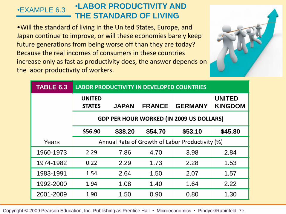
•Will the standard of living in the United States, Europe, and Japan continue to improve, or will these economies barely keep future generations from being worse off than they are today? Because the real incomes of consumers in these countries increase only as fast as productivity does, the answer depends on the labor productivity of workers.
•EXAMPLE 6.3 •LABOR PRODUCTIVITY AND
THE STANDARD OF LIVING
TABLE 6.3 LABOR PRODUCTIVITY IN DEVELOPED COUNTRIES
UNITED STATES JAPAN FRANCE GERMANY
UNITED
KINGDOM
GDP PER HOUR WORKED (IN 2009 US DOLLARS)
$56.90 $38.20 $54.70 $53.10 $45.80
Years Annual Rate of Growth of Labor Productivity (%)
1960-1973 2.29 7.86 4.70 3.98 2.84
1974-1982 0.22 2.29 1.73 2.28 1.53
1983-1991 1.54 2.64 1.50 2.07 1.57
1992-2000 1.94 1.08 1.40 1.64 2.22
2001-2009 1.90 1.50 0.90 0.80 1.30
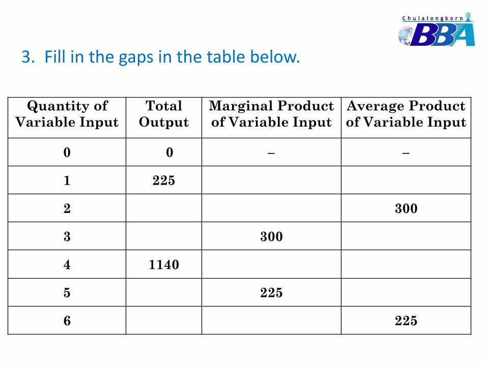
3. Fill in the gaps in the table below.
Quantity of
Variable Input
Total
Output
Marginal Product
of Variable Input
Average Product
of Variable Input
0 0 – –
1 225
2 300
3 300
4 1140
5 225
6 225
Copyright © 2009 Pearson Education, Inc. Publishing as Prentice Hall • Microeconomics • Pindyck/Rubinfeld, 7e.
Quantity of
Variable Input
Total
Output
Marginal Product
of Variable Input
Average Product
of Variable Input
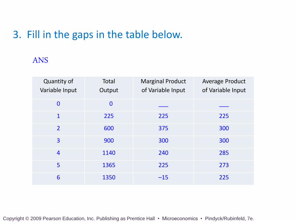
0 0 ___ ___
1 225 225 225
2 600 375 300
3 900 300 300
4 1140 240 285
5 1365 225 273
6 1350 –15 225
3. Fill in the gaps in the table below.
ANS
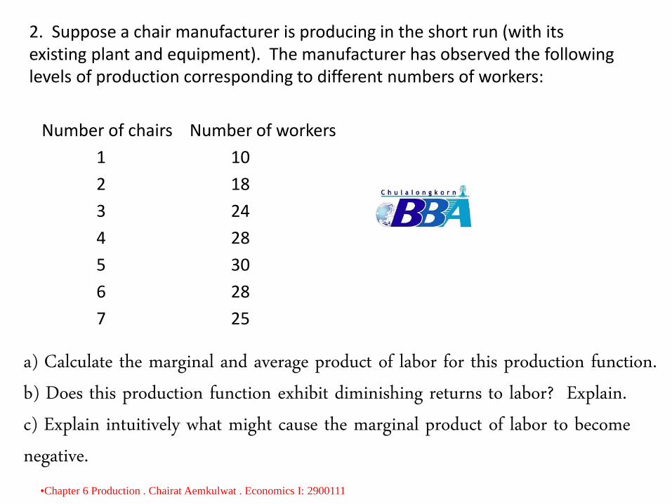
2. Suppose a chair manufacturer is producing in the short run (with its existing plant and equipment). The manufacturer has observed the following levels of production corresponding to different numbers of workers:
Number of chairs Number of workers
1 10
2 18
3 24
4 28
5 30
6 28
7 25
a) Calculate the marginal and average product of labor for this production function.b) Does this production function exhibit diminishing returns to labor? Explain.c) Explain intuitively what might cause the marginal product of labor to become negative.
•Chapter 6 Production . Chairat Aemkulwat . Economics I: 2900111
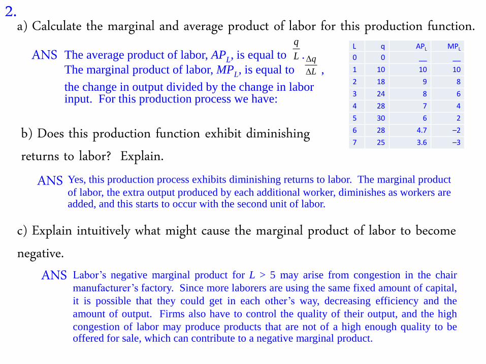
a) Calculate the marginal and average product of labor for this production function.2.
b) Does this production function exhibit diminishing returns to labor? Explain.
c) Explain intuitively what might cause the marginal product of labor to become negative.
The average product of labor, APL, is equal to .
The marginal product of labor, MPL, is equal to ,
the change in output divided by the change in labor input. For this production process we have:
L
q
L
q
ANS L q APL MPL
0 0 __ __
1 10 10 10
2 18 9 8
3 24 8 6
4 28 7 4
5 30 6 2
6 28 4.7 –2
7 25 3.6 –3
Yes, this production process exhibits diminishing returns to labor. The marginal product
of labor, the extra output produced by each additional worker, diminishes as workers areadded, and this starts to occur with the second unit of labor.
Labor’s negative marginal product for L > 5 may arise from congestion in the chair
manufacturer’s factory. Since more laborers are using the same fixed amount of capital,
it is possible that they could get in each other’s way, decreasing efficiency and the
amount of output. Firms also have to control the quality of their output, and the high
congestion of labor may produce products that are not of a high enough quality to beoffered for sale, which can contribute to a negative marginal product.
ANS
ANS
LABOR INPUT
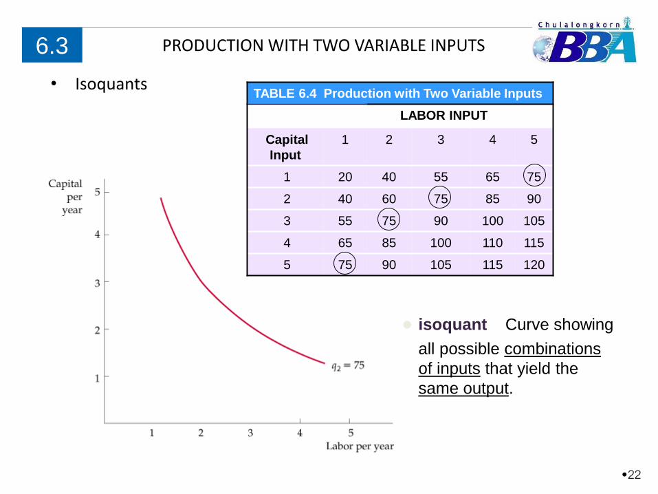
PRODUCTION WITH TWO VARIABLE INPUTS
• Isoquants
6.3
TABLE 6.4 Production with Two Variable Inputs
Capital
Input
1 2 3 4 5
1 20 40 55 65 75
2 40 60 75 85 90
3 55 75 90 100 105
4 65 85 100 110 115
5 75 90 105 115 120
● isoquant Curve showing
all possible combinations
of inputs that yield the
same output.
•22
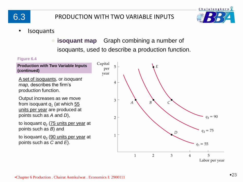
PRODUCTION WITH TWO VARIABLE INPUTS
• Isoquants
6.3
● isoquant map Graph combining a number of
isoquants, used to describe a production function.
A set of isoquants, or isoquant
map, describes the firm’s
production function.
Output increases as we move
from isoquant q1 (at which 55
units per year are produced at
points such as A and D),
to isoquant q2 (75 units per year at
points such as B) and
to isoquant q3 (90 units per year at
points such as C and E).
Production with Two Variable Inputs
(continued)
Figure 6.4
•23•Chapter 6 Production . Chairat Aemkulwat . Economics I: 2900111
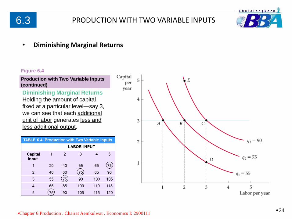
PRODUCTION WITH TWO VARIABLE INPUTS
• Diminishing Marginal Returns
6.3
Diminishing Marginal Returns
Holding the amount of capital
fixed at a particular level—say 3,
we can see that each additional
unit of labor generates less and
less additional output.
Production with Two Variable Inputs
(continued)
Figure 6.4
•24•Chapter 6 Production . Chairat Aemkulwat . Economics I: 2900111
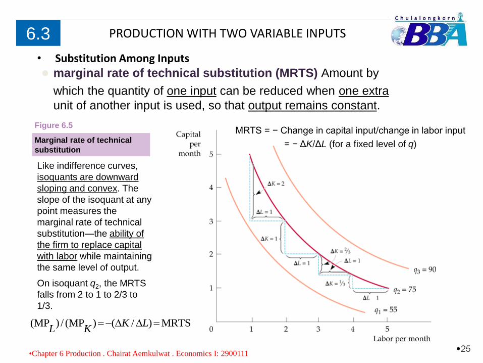
PRODUCTION WITH TWO VARIABLE INPUTS
• Substitution Among Inputs
6.3
Like indifference curves,
isoquants are downward
sloping and convex. The
slope of the isoquant at any
point measures the
marginal rate of technical
substitution—the ability of
the firm to replace capital
with labor while maintaining
the same level of output.
On isoquant q2, the MRTS
falls from 2 to 1 to 2/3 to
1/3.
Marginal rate of technical
substitution
Figure 6.5
● marginal rate of technical substitution (MRTS) Amount by
which the quantity of one input can be reduced when one extra
unit of another input is used, so that output remains constant.
MRTS = − Change in capital input/change in labor input
= − ΔK/ΔL (for a fixed level of q)
(MP )/ (MP ) ( / ) MRTSK LL K
•25•Chapter 6 Production . Chairat Aemkulwat . Economics I: 2900111
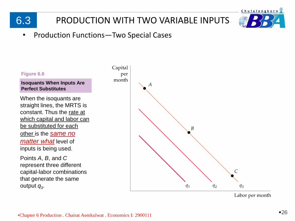
PRODUCTION WITH TWO VARIABLE INPUTS
• Production Functions—Two Special Cases
6.3
When the isoquants are
straight lines, the MRTS is
constant. Thus the rate at
which capital and labor can
be substituted for each
other is the same no
matter what level of
inputs is being used.
Points A, B, and C
represent three different
capital-labor combinations
that generate the same
output q3.
Isoquants When Inputs Are
Perfect Substitutes
Figure 6.6
•26•Chapter 6 Production . Chairat Aemkulwat . Economics I: 2900111
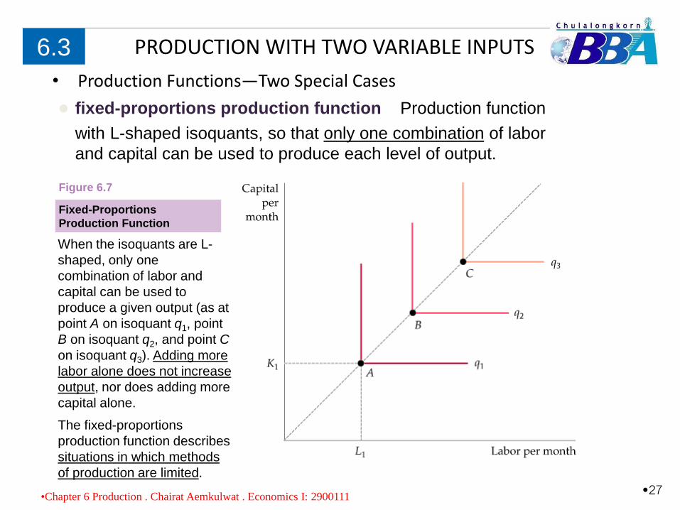
PRODUCTION WITH TWO VARIABLE INPUTS
• Production Functions—Two Special Cases
6.3
When the isoquants are L-
shaped, only one
combination of labor and
capital can be used to
produce a given output (as at
point A on isoquant q1, point
B on isoquant q2, and point C
on isoquant q3). Adding more
labor alone does not increase
output, nor does adding more
capital alone.
The fixed-proportions
production function describes
situations in which methods
of production are limited.
Fixed-Proportions
Production Function
Figure 6.7
● fixed-proportions production function Production function
with L-shaped isoquants, so that only one combination of labor
and capital can be used to produce each level of output.
•27•Chapter 6 Production . Chairat Aemkulwat . Economics I: 2900111
Copyright © 2009 Pearson Education, Inc. Publishing as Prentice Hall • Microeconomics • Pindyck/Rubinfeld, 7e.
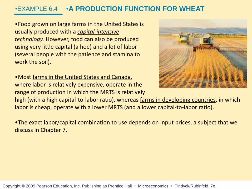
•Food grown on large farms in the United States isusually produced with a capital-intensivetechnology. However, food can also be producedusing very little capital (a hoe) and a lot of labor(several people with the patience and stamina towork the soil).
•Most farms in the United States and Canada,where labor is relatively expensive, operate in therange of production in which the MRTS is relativelyhigh (with a high capital-to-labor ratio), whereas farms in developing countries, in which labor is cheap, operate with a lower MRTS (and a lower capital-to-labor ratio).
•The exact labor/capital combination to use depends on input prices, a subject that we discuss in Chapter 7.
•EXAMPLE 6.4 •A PRODUCTION FUNCTION FOR WHEAT
Copyright © 2009 Pearson Education, Inc. Publishing as Prentice Hall • Microeconomics • Pindyck/Rubinfeld, 7e.
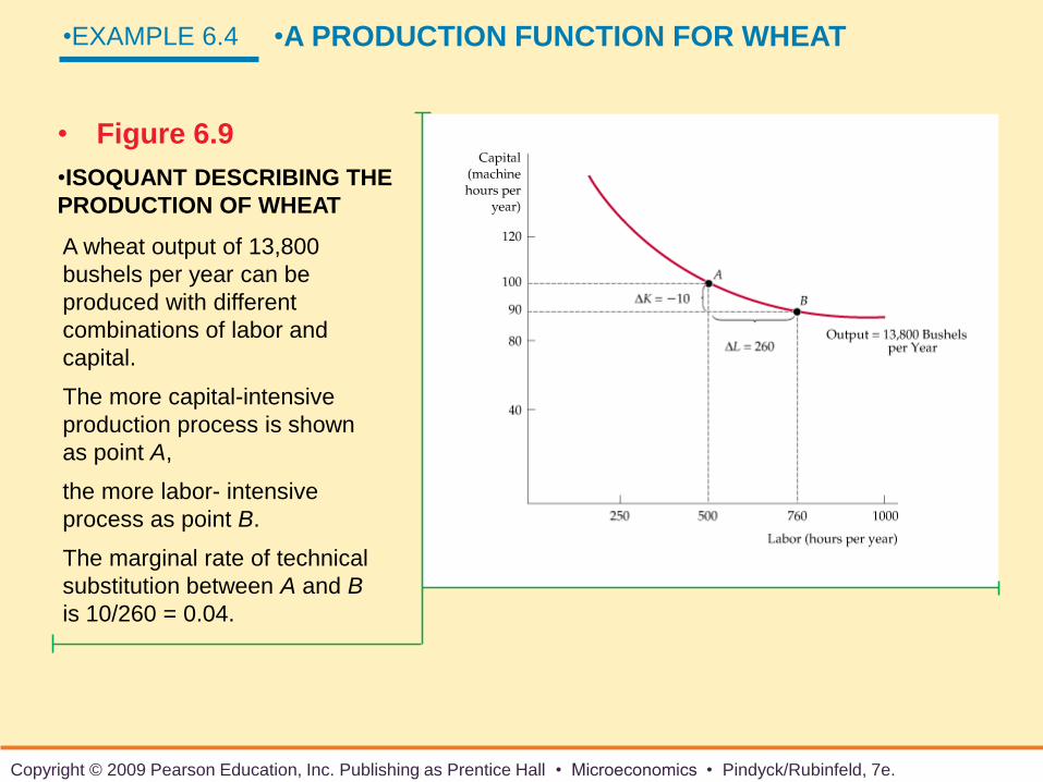
•EXAMPLE 6.4 •A PRODUCTION FUNCTION FOR WHEAT
•ISOQUANT DESCRIBING THE
PRODUCTION OF WHEAT
• Figure 6.9
A wheat output of 13,800
bushels per year can be
produced with different
combinations of labor and
capital.
The more capital-intensive
production process is shown
as point A,
the more labor- intensive
process as point B.
The marginal rate of technical
substitution between A and B
is 10/260 = 0.04.
Copyright © 2009 Pearson Education, Inc. Publishing as Prentice Hall • Microeconomics • Pindyck/Rubinfeld, 7e.
5. For each of the following examples, draw a representative
isoquant. What can you say about the marginal rate of
technical substitution in each case?
a) A firm can hire only full-time employees to produce its output, or it can hire some combination of full-time and part-time employees. For each full-time worker let go, the firm must hire an increasing number of temporary employees to maintain the same level of output.
b) A firm finds that it can always trade two units of labor for one unit of capital and still keep output constant.
c) A firm requires exactly two full-time workers to operate each piece of machinery in the factory
Copyright © 2009 Pearson Education, Inc. Publishing as Prentice Hall • Microeconomics • Pindyck/Rubinfeld, 7e.
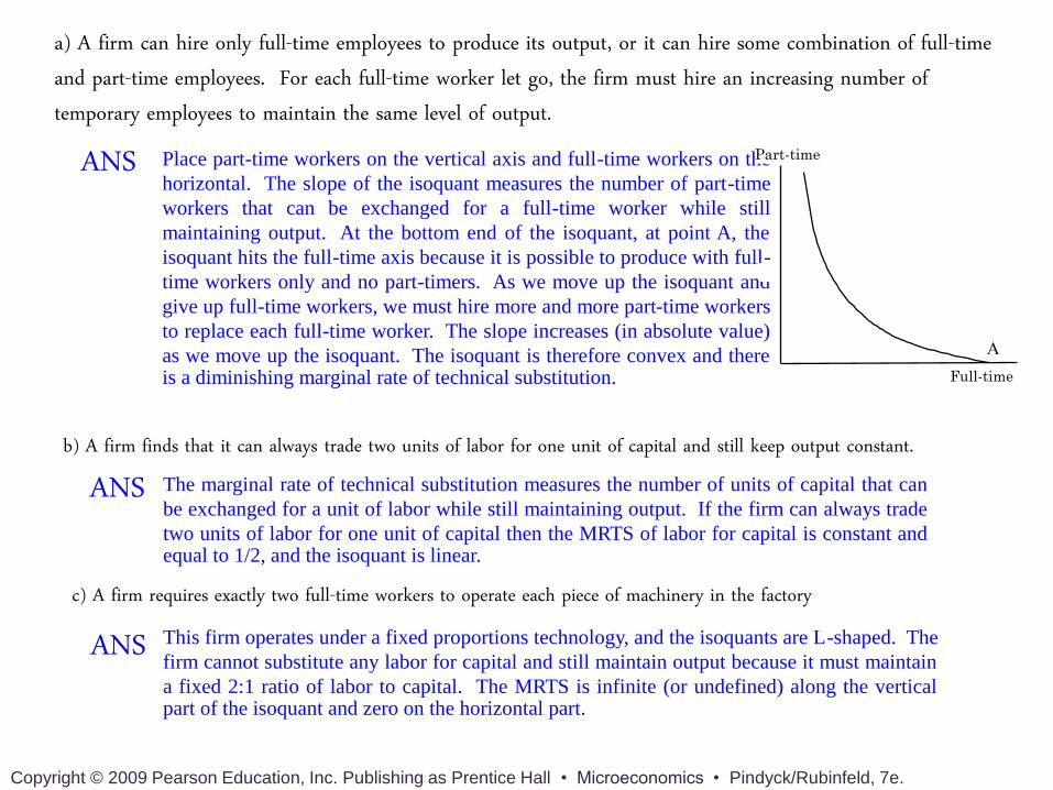
a) A firm can hire only full-time employees to produce its output, or it can hire some combination of full-time and part-time employees. For each full-time worker let go, the firm must hire an increasing number of temporary employees to maintain the same level of output.
c) A firm requires exactly two full-time workers to operate each piece of machinery in the factory
b) A firm finds that it can always trade two units of labor for one unit of capital and still keep output constant.
Place part-time workers on the vertical axis and full-time workers on the
horizontal. The slope of the isoquant measures the number of part-time
workers that can be exchanged for a full-time worker while still
maintaining output. At the bottom end of the isoquant, at point A, the
isoquant hits the full-time axis because it is possible to produce with full-
time workers only and no part-timers. As we move up the isoquant and
give up full-time workers, we must hire more and more part-time workers
to replace each full-time worker. The slope increases (in absolute value)
as we move up the isoquant. The isoquant is therefore convex and there is a diminishing marginal rate of technical substitution.
Full-time
A
Part-time
ANS
The marginal rate of technical substitution measures the number of units of capital that can
be exchanged for a unit of labor while still maintaining output. If the firm can always trade
two units of labor for one unit of capital then the MRTS of labor for capital is constant and equal to 1/2, and the isoquant is linear.
This firm operates under a fixed proportions technology, and the isoquants are L-shaped. The
firm cannot substitute any labor for capital and still maintain output because it must maintain
a fixed 2:1 ratio of labor to capital. The MRTS is infinite (or undefined) along the vertical part of the isoquant and zero on the horizontal part.
ANS
ANS
Copyright © 2009 Pearson Education, Inc. Publishing as Prentice Hall • Microeconomics • Pindyck/Rubinfeld, 7e.
6. A firm has a production process in which the inputs to production are perfectly substitutable in the long run. Can you tell whether the marginal rate of technical substitution is high or low, or is further information necessary? Discuss.
Further information is necessary. The marginal rate of technical
substitution, MRTS, is the absolute value of the slope of an isoquant.
If the inputs are perfect substitutes, the isoquants will be linear. To
calculate the slope of the isoquant, and hence the MRTS, we need to
know the rate at which one input may be substituted for the other. In
this case, we do not know whether the MRTS is high or low. All we
know is that it is a constant number. We need to know the marginalproduct of each input to determine the MRTS.
ANS
RETURNS TO SCALE6.4
● returns to scale Rate at which output increases as
inputs are increased proportionately.
● increasing returns to scale Situation in which output
more than doubles when all inputs are doubled.
● constant returns to scale Situation in which output
doubles when all inputs are doubled.
● decreasing returns to scale Situation in which output
less than doubles when all inputs are doubled.
•33•Chapter 6 Production . Chairat Aemkulwat . Economics I: 2900111
RETURNS TO SCALE
• Describing Returns to Scale
6.4
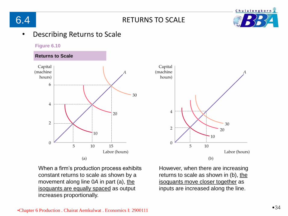
When a firm’s production process exhibits
constant returns to scale as shown by a
movement along line 0A in part (a), the
isoquants are equally spaced as output
increases proportionally.
Returns to Scale
Figure 6.10
However, when there are increasing
returns to scale as shown in (b), the
isoquants move closer together as
inputs are increased along the line.
•34•Chapter 6 Production . Chairat Aemkulwat . Economics I: 2900111
Copyright © 2009 Pearson Education, Inc. Publishing as Prentice Hall • Microeconomics • Pindyck/Rubinfeld, 7e.
• Describing Returns to Scale
•Returns to scale need not be uniform across all possible levels ofoutput. For example, at lower levels of output, the firm could have increasing returns to scale, but constant and eventually decreasing returns at higher levels of output.
•In Figure 6.10 (a), the firm’s production function exhibits constant returns. Twice as much of both inputs is needed to produce 20 units, and three times as much is needed to produce 30 units.
•In Figure 6.10 (b), the firm’s production function exhibits increasing returns to scale. Less than twice the amount of both inputs is needed to increase production from 10 units to 20; substantially less than three times the inputs are needed to produce 30 units.
•Returns to scale vary considerably across firms and industries. Other things being equal, the greater the returns to scale, the larger the firms in an industry are likely to be.
Copyright © 2009 Pearson Education, Inc. Publishing as Prentice Hall • Microeconomics • Pindyck/Rubinfeld, 7e.
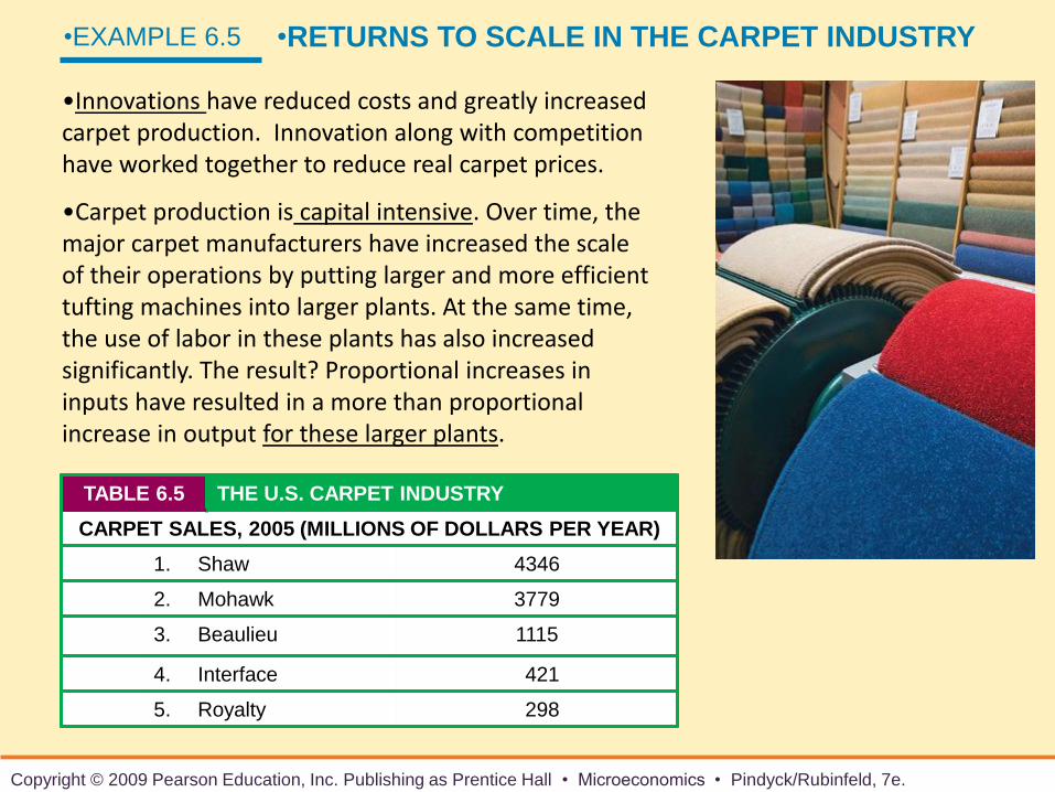
•Innovations have reduced costs and greatly increasedcarpet production. Innovation along with competitionhave worked together to reduce real carpet prices.
•Carpet production is capital intensive. Over time, themajor carpet manufacturers have increased the scaleof their operations by putting larger and more efficienttufting machines into larger plants. At the same time,the use of labor in these plants has also increasedsignificantly. The result? Proportional increases ininputs have resulted in a more than proportionalincrease in output for these larger plants.
•EXAMPLE 6.5 •RETURNS TO SCALE IN THE CARPET INDUSTRY
TABLE 6.5 THE U.S. CARPET INDUSTRY
CARPET SALES, 2005 (MILLIONS OF DOLLARS PER YEAR)
1. Shaw 4346
2. Mohawk 3779
3. Beaulieu 1115
4. Interface 421
5. Royalty 298
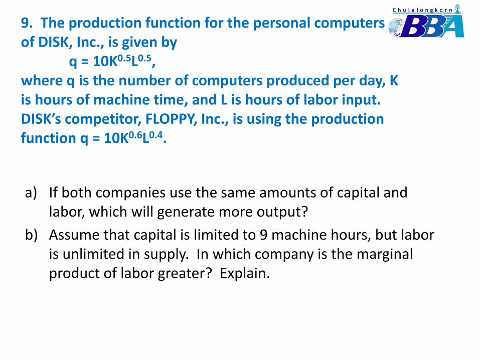
9. The production function for the personal computers of DISK, Inc., is given by
q = 10K0.5L0.5, where q is the number of computers produced per day, K is hours of machine time, and L is hours of labor input. DISK’s competitor, FLOPPY, Inc., is using the production function q = 10K0.6L0.4.
a) If both companies use the same amounts of capital and labor, which will generate more output?
b) Assume that capital is limited to 9 machine hours, but labor is unlimited in supply. In which company is the marginal product of labor greater? Explain.
Copyright © 2009 Pearson Education, Inc. Publishing as Prentice Hall • Microeconomics • Pindyck/Rubinfeld, 7e.
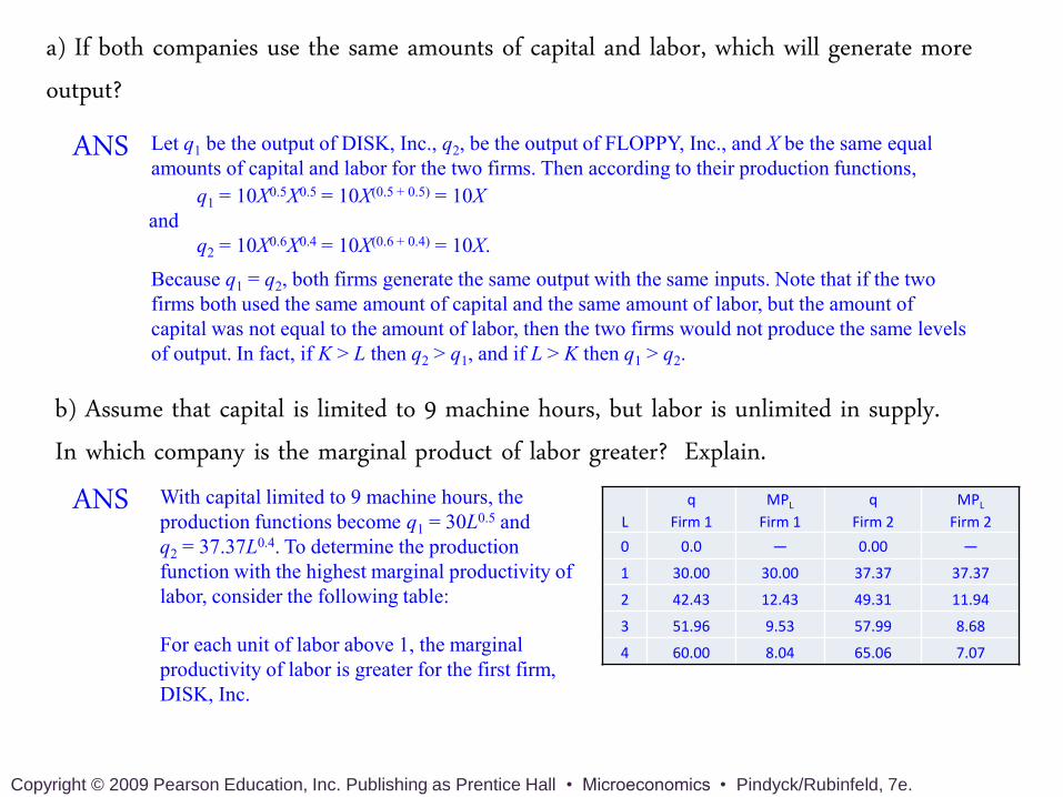
Let q1 be the output of DISK, Inc., q2, be the output of FLOPPY, Inc., and X be the same equal
amounts of capital and labor for the two firms. Then according to their production functions,
q1 = 10X0.5X0.5 = 10X(0.5 + 0.5) = 10X
and
q2 = 10X0.6X0.4 = 10X(0.6 + 0.4) = 10X.
Because q1 = q2, both firms generate the same output with the same inputs. Note that if the two
firms both used the same amount of capital and the same amount of labor, but the amount of
capital was not equal to the amount of labor, then the two firms would not produce the same levels
of output. In fact, if K > L then q2 > q1, and if L > K then q1 > q2.
a) If both companies use the same amounts of capital and labor, which will generate more output?
b) Assume that capital is limited to 9 machine hours, but labor is unlimited in supply. In which company is the marginal product of labor greater? Explain.
With capital limited to 9 machine hours, the
production functions become q1 = 30L0.5 and
q2 = 37.37L0.4. To determine the production
function with the highest marginal productivity of
labor, consider the following table:
For each unit of labor above 1, the marginal
productivity of labor is greater for the first firm,
DISK, Inc.
L
q
Firm 1
MPL
Firm 1
q
Firm 2
MPL
Firm 2
0 0.0 — 0.00 —
1 30.00 30.00 37.37 37.37
2 42.43 12.43 49.31 11.94
3 51.96 9.53 57.99 8.68
4 60.00 8.04 65.06 7.07
ANS
ANS
Copyright © 2009 Pearson Education, Inc. Publishing as Prentice Hall • Microeconomics • Pindyck/Rubinfeld, 7e.
Recap CHAPTER 6
• The Technology of Production
• Production with One Variable Input (Labor)
• Production with Two Variable Inputs
• Returns to Scale
•Chapter 6 Production . Chairat Aemkulwat . Economics I: 2900111