Embed Size (px)
Citation preview

Chapter 6: Modeling Transient Compressible Flow
This tutorial is divided into the following sections:
6.1. Introduction
6.2. Prerequisites
6.3. Problem Description
6.4. Setup and Solution
6.5. Summary
6.6. Further Improvements
6.1. Introduction
In this tutorial, ANSYS Fluent’s density-based implicit solver is used to predict the time-dependent flow
through a two-dimensional nozzle. As an initial condition for the transient problem, a steady-state
solution is generated to provide the initial values for the mass flow rate at the nozzle exit.
This tutorial demonstrates how to do the following:
• Calculate a steady-state solution (using the density-based implicit solver) as an initial condition for a
transient flow prediction.
• Define a transient boundary condition using a user-defined function (UDF).
• Use dynamic mesh adaption for both steady-state and transient flows.
• Calculate a transient solution using the second-order implicit transient formulation and the density-based
implicit solver.
• Create an animation of the transient flow using ANSYS Fluent’s transient solution animation feature.
6.2. Prerequisites
This tutorial is written with the assumption that you have completed one or more of the introductory
tutorials found in this manual:
• Introduction to Using ANSYS Fluent in ANSYS Workbench: Fluid Flow and Heat Transfer in a Mixing
Elbow (p. 1)
• Parametric Analysis in ANSYS Workbench Using ANSYS Fluent (p. 73)
• Introduction to Using ANSYS Fluent: Fluid Flow and Heat Transfer in a Mixing Elbow (p. 123)
and that you are familiar with the ANSYS Fluent navigation pane and menu structure. Some steps in
the setup and solution procedure will not be shown explicitly.
257Release 15.0 - © SAS IP, Inc. All rights reserved. - Contains proprietary and confidential information
of ANSYS, Inc. and its subsidiaries and affiliates.

6.3. Problem Description
The geometry to be considered in this tutorial is shown in Figure 6.1: Problem Specification (p. 258).
Flow through a simple nozzle is simulated as a 2D planar model. The nozzle has an inlet height of 0.2
m, and the nozzle contours have a sinusoidal shape that produces a 20% reduction in flow area. Due
to symmetry, only half of the nozzle is modeled.
Figure 6.1: Problem Specification
6.4. Setup and Solution
The following sections describe the setup and solution steps for this tutorial:
6.4.1. Preparation
6.4.2. Reading and Checking the Mesh
6.4.3. Specifying Solver and Analysis Type
6.4.4. Specifying the Models
6.4.5. Editing the Material Properties
6.4.6. Setting the Operating Conditions
6.4.7. Creating the Boundary Conditions
6.4.8. Setting the Solution Parameters for Steady Flow and Solving
6.4.9. Enabling Time Dependence and Setting Transient Conditions
6.4.10. Specifying Solution Parameters for Transient Flow and Solving
6.4.11. Saving and Postprocessing Time-Dependent Data Sets
6.4.1. Preparation
To prepare for running this tutorial:
1. Set up a working folder on the computer you will be using.
2. Go to the ANSYS Customer Portal, https://support.ansys.com/training.
Note
If you do not have a login, you can request one by clicking Customer Registration on
the log in page.
3. Enter the name of this tutorial into the search bar.
4. Narrow the results by using the filter on the left side of the page.
Release 15.0 - © SAS IP, Inc. All rights reserved. - Contains proprietary and confidential informationof ANSYS, Inc. and its subsidiaries and affiliates.258
Modeling Transient Compressible Flow

a. Click ANSYS Fluent under Product.
b. Click 15.0 under Version.
5. Select this tutorial from the list.
6. Click Files to download the input and solution files.
7. Unzip the �������������������������� file you downloaded to your working folder.
The files ���������� and ������� can be found in the ��������������������� folder created
after unzipping the file.
8. Use Fluent Launcher to start the 2D version of ANSYS Fluent.
Fluent Launcher displays your Display Options preferences from the previous session.
For more information about Fluent Launcher, see Starting ANSYS Fluent Using Fluent Launcher in
the Getting Started Guide.
9. Ensure that the Display Mesh After Reading, Embed Graphics Windows, and Workbench ColorScheme options are enabled.
10. Ensure that the Serial
11. Disable the Double Precision option.
6.4.2. Reading and Checking the Mesh
1. Read the mesh file ����������.
File → Read → Mesh...
The mesh for the half of the geometry is displayed in the graphics window.
2. Check the mesh.
General → Check
ANSYS Fluent will perform various checks on the mesh and will report the progress in the console window.
Ensure that the reported minimum volume is a positive number.
3. Verify that the mesh size is correct.
General → Scale...
259Release 15.0 - © SAS IP, Inc. All rights reserved. - Contains proprietary and confidential information
of ANSYS, Inc. and its subsidiaries and affiliates.
Setup and Solution
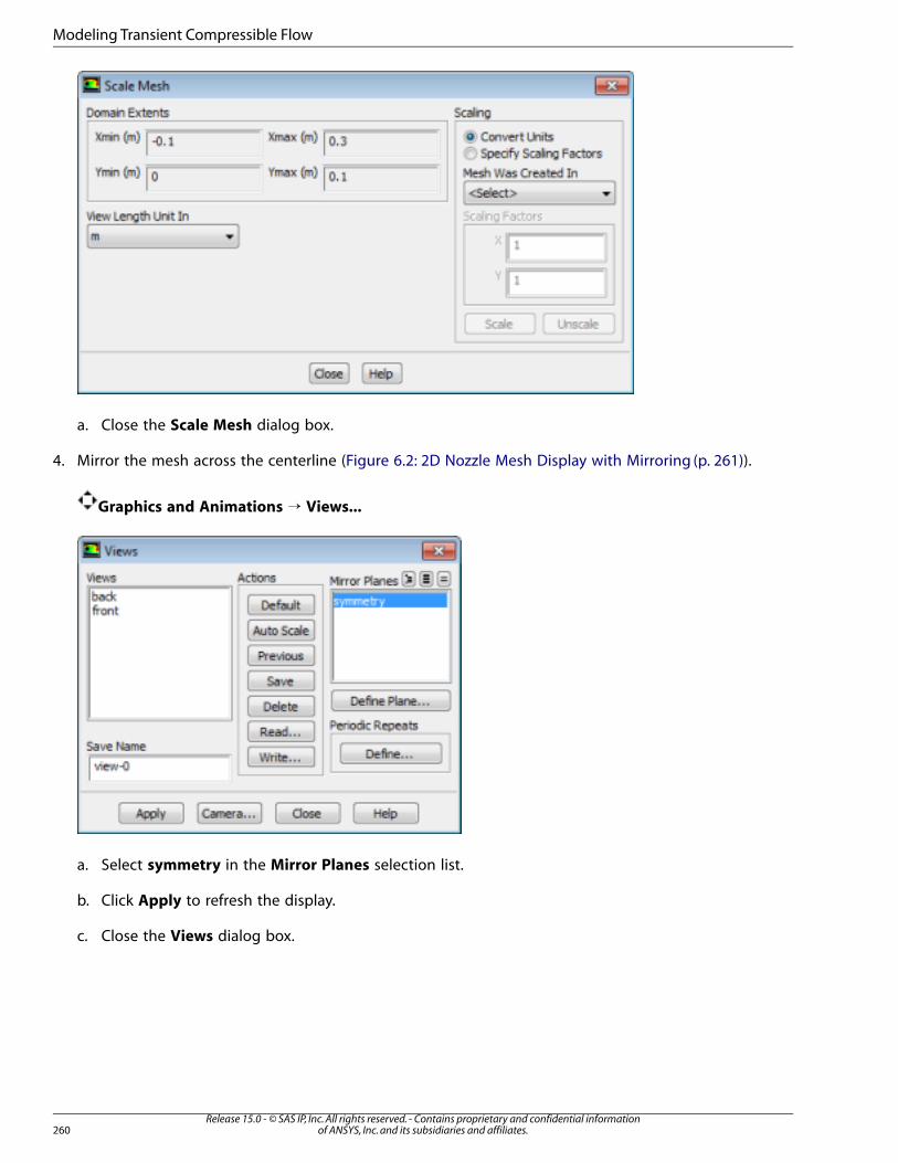
a. Close the Scale Mesh dialog box.
4. Mirror the mesh across the centerline (Figure 6.2: 2D Nozzle Mesh Display with Mirroring (p. 261)).
Graphics and Animations → Views...
a. Select symmetry in the Mirror Planes selection list.
b. Click Apply to refresh the display.
c. Close the Views dialog box.
Release 15.0 - © SAS IP, Inc. All rights reserved. - Contains proprietary and confidential informationof ANSYS, Inc. and its subsidiaries and affiliates.260
Modeling Transient Compressible Flow
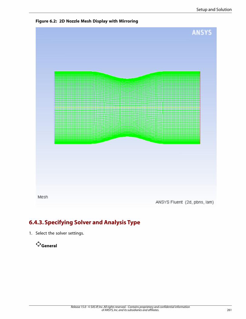
Figure 6.2: 2D Nozzle Mesh Display with Mirroring
6.4.3. Specifying Solver and Analysis Type
1. Select the solver settings.
General
261Release 15.0 - © SAS IP, Inc. All rights reserved. - Contains proprietary and confidential information
of ANSYS, Inc. and its subsidiaries and affiliates.
Setup and Solution

a. Select Density-Based from the Type list in the Solver group box.
The density-based implicit solver is the solver of choice for compressible, transonic flows without
significant regions of low-speed flow. In cases with significant low-speed flow regions, the pressure-
based solver is preferred. Also, for transient cases with traveling shocks, the density-based explicit
solver with explicit time stepping may be the most efficient.
b. Retain the default selection of Steady from the Time list.
Note
You will solve for the steady flow through the nozzle initially. In later steps, you will
use these initial results as a starting point for a transient calculation.
2. For convenience, change the unit of measurement for pressure.
General → Units...
The pressure for this problem is specified in atm, which is not the default unit in ANSYS Fluent. You must
redefine the pressure unit as atm.
Release 15.0 - © SAS IP, Inc. All rights reserved. - Contains proprietary and confidential informationof ANSYS, Inc. and its subsidiaries and affiliates.262
Modeling Transient Compressible Flow

a. Select pressure in the Quantities selection list.
Scroll down the list to find pressure.
b. Select atm in the Units selection list.
c. Close the Set Units dialog box.
6.4.4. Specifying the Models
1. Enable the energy equation.
Models → Energy → Edit...
2. Select the k-omega SST turbulence model.
Models → Viscous → Edit...
263Release 15.0 - © SAS IP, Inc. All rights reserved. - Contains proprietary and confidential information
of ANSYS, Inc. and its subsidiaries and affiliates.
Setup and Solution

a. Select k-omega (2eqn) in the Model list.
b. Select SST in the k-omega Model group box.
c. Click OK to close the Viscous Model dialog box.
6.4.5. Editing the Material Properties
1. Set the properties for air, the default fluid material.
Materials → air → Create/Edit...
Release 15.0 - © SAS IP, Inc. All rights reserved. - Contains proprietary and confidential informationof ANSYS, Inc. and its subsidiaries and affiliates.264
Modeling Transient Compressible Flow

a. Select ideal-gas from the Density drop-down list in the Properties group box, so that the ideal gas
law is used to calculate density.
Note
ANSYS Fluent automatically enables the solution of the energy equation when the
ideal gas law is used, in case you did not already enable it manually in the Energydialog box.
b. Retain the default values for all other properties.
c. Click the Change/Create button to save your change.
d. Close the Create/Edit Materials dialog box.
6.4.6. Setting the Operating Conditions
1. Set the operating pressure.
Boundary Conditions → Operating Conditions...
265Release 15.0 - © SAS IP, Inc. All rights reserved. - Contains proprietary and confidential information
of ANSYS, Inc. and its subsidiaries and affiliates.
Setup and Solution

a. Enter � atm for Operating Pressure.
b. Click OK to close the Operating Conditions dialog box.
Since you have set the operating pressure to zero, you will specify the boundary condition inputs for
pressure in terms of absolute pressures when you define them in the next step. Boundary condition inputs
for pressure should always be relative to the value used for operating pressure.
6.4.7. Creating the Boundary Conditions
1. Set the boundary conditions for the nozzle inlet (inlet).
Boundary Conditions → inlet → Edit...
Release 15.0 - © SAS IP, Inc. All rights reserved. - Contains proprietary and confidential informationof ANSYS, Inc. and its subsidiaries and affiliates.266
Modeling Transient Compressible Flow

a. Enter ��� atm for Gauge Total Pressure.
b. Enter ������ atm for Supersonic/Initial Gauge Pressure.
The inlet static pressure estimate is the mean pressure at the nozzle exit. This value will be used during
the solution initialization phase to provide a guess for the nozzle velocity.
c. Retain Intensity and Viscosity Ratio from the Specification Method drop-down list in the Turbulencegroup box.
d. Enter ���% for Turbulent Intensity.
e. Retain the setting of �� for Turbulent Viscosity Ratio.
f. Click OK to close the Pressure Inlet dialog box.
2. Set the boundary conditions for the nozzle exit (outlet).
Boundary Conditions → outlet → Edit...
267Release 15.0 - © SAS IP, Inc. All rights reserved. - Contains proprietary and confidential information
of ANSYS, Inc. and its subsidiaries and affiliates.
Setup and Solution

a. Enter ������ atm for Gauge Pressure.
b. Retain Intensity and Viscosity Ratio from the Specification Method drop-down list in the Turbulencegroup box.
c. Enter ���% for Backflow Turbulent Intensity.
d. Retain the setting of �� for Backflow Turbulent Viscosity Ratio.
If substantial backflow occurs at the outlet, you may need to adjust the backflow values to levels
close to the actual exit conditions.
e. Click OK to close the Pressure Outlet dialog box.
6.4.8. Setting the Solution Parameters for Steady Flow and Solving
In this step, you will generate a steady-state flow solution that will be used as an initial condition for the
time-dependent solution.
1. Set the solution parameters.
Solution Methods
Release 15.0 - © SAS IP, Inc. All rights reserved. - Contains proprietary and confidential informationof ANSYS, Inc. and its subsidiaries and affiliates.268
Modeling Transient Compressible Flow

a. Retain the default selection of Least Squares Cell Based from the Gradient drop-down list in the
Spatial Discretization group box.
b. Select Second Order Upwind from the Turbulent Kinetic Energy and Specific Dissipation Ratedrop-down lists.
Second-order discretization provides optimum accuracy.
2. Modify the Courant Number.
Solution Controls
269Release 15.0 - © SAS IP, Inc. All rights reserved. - Contains proprietary and confidential information
of ANSYS, Inc. and its subsidiaries and affiliates.
Setup and Solution

a. Set the Courant Number to ��.
Note
The default Courant number for the density-based implicit formulation is 5. For relat-
ively simple problems, setting the Courant number to 10, 20, 100, or even higher
value may be suitable and produce fast and stable convergence. However, if you en-
counter convergence difficulties at the startup of the simulation of a properly set up
problem, then you should consider setting the Courant number to its default value
of 5. As the solution progresses, you can start to gradually increase the Courant
number until the final convergence is reached.
b. Retain the default values for the Under-Relaxation Factors.
3. Enable the plotting of residuals.
Monitors → Residuals → Edit...
Release 15.0 - © SAS IP, Inc. All rights reserved. - Contains proprietary and confidential informationof ANSYS, Inc. and its subsidiaries and affiliates.270
Modeling Transient Compressible Flow

a. Ensure that Plot is enabled in the Options group box.
b. Select none from the Convergence Criterion drop-down list.
c. Click OK to close the Residual Monitors dialog box.
4. Enable the plotting of mass flow rate at the flow exit.
Monitors (Surface Monitors) → Create...
271Release 15.0 - © SAS IP, Inc. All rights reserved. - Contains proprietary and confidential information
of ANSYS, Inc. and its subsidiaries and affiliates.
Setup and Solution
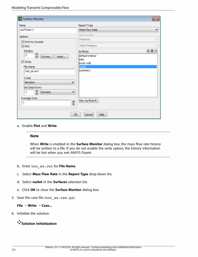
a. Enable Plot and Write.
Note
When Write is enabled in the Surface Monitor dialog box, the mass flow rate history
will be written to a file. If you do not enable the write option, the history information
will be lost when you exit ANSYS Fluent.
b. Enter ���������� for File Name.
c. Select Mass Flow Rate in the Report Type drop-down list.
d. Select outlet in the Surfaces selection list.
e. Click OK to close the Surface Monitor dialog box.
5. Save the case file (�������������).
File → Write → Case...
6. Initialize the solution.
Solution Initialization
Release 15.0 - © SAS IP, Inc. All rights reserved. - Contains proprietary and confidential informationof ANSYS, Inc. and its subsidiaries and affiliates.272
Modeling Transient Compressible Flow

a. Retain the default selection of Hybrid Initialization from the Initialization Methods group box.
b. Click Initialize.
7. Set up gradient adaption for dynamic mesh refinement.
Adapt → Gradient...
You will enable dynamic adaption so that the solver periodically refines the mesh in the vicinity of the
shocks as the iterations progress. The shocks are identified by their large pressure gradients.
a. Select Gradient from the Method group box.
The mesh adaption criterion can either be the gradient or the curvature (second gradient). Because
strong shocks occur inside the nozzle, the gradient is used as the adaption criterion.
b. Select Scale from the Normalization group box.
Mesh adaption can be controlled by the raw (or standard) value of the gradient, the scaled value (by
its average in the domain), or the normalized value (by its maximum in the domain). For dynamic
273Release 15.0 - © SAS IP, Inc. All rights reserved. - Contains proprietary and confidential information
of ANSYS, Inc. and its subsidiaries and affiliates.
Setup and Solution

mesh adaption, it is recommended that you use either the scaled or normalized value because the
raw values will probably change strongly during the computation, which would necessitate a read-
justment of the coarsen and refine thresholds. In this case, the scaled gradient is used.
c. Enable Dynamic in the Dynamic group box.
d. Enter ��� for the Interval.
For steady-state flows, it is sufficient to only seldomly adapt the mesh—in this case an interval of
100 iterations is chosen. For time-dependent flows, a considerably smaller interval must be used.
e. Retain the default selection of Pressure... and Static Pressure from the Gradients of drop-down
lists.
f. Enter ��� for Coarsen Threshold.
g. Enter ��� for Refine Threshold.
As the refined regions of the mesh get larger, the coarsen and refine thresholds should get smaller.
A coarsen threshold of 0.3 and a refine threshold of 0.7 result in a “medium” to “strong” mesh refine-
ment in combination with the scaled gradient.
h. Click Apply to store the information.
i. Click the Controls... button to open the Mesh Adaption Controls dialog box.
i. Retain the default selection of fluid in the Zones selection list.
ii. Enter ����� for Max # of Cells.
To restrict the mesh adaption, the maximum number of cells can be limited. If this limit is violated
during the adaption, the coarsen and refine thresholds are adjusted to respect the maximum
number of cells. Additional restrictions can be placed on the minimum cell volume, minimum
number of cells, and maximum level of refinement.
iii. Click OK to save your settings and close the Mesh Adaption Controls dialog box.
Release 15.0 - © SAS IP, Inc. All rights reserved. - Contains proprietary and confidential informationof ANSYS, Inc. and its subsidiaries and affiliates.274
Modeling Transient Compressible Flow

j. Click Close to close the Gradient Adaption dialog box.
8. Start the calculation by requesting ��� iterations.
Run Calculation
a. Enter 500 for Number of Iterations.
b. Click Calculate to start the steady flow simulation.
Figure 6.3: Mass Flow Rate History
275Release 15.0 - © SAS IP, Inc. All rights reserved. - Contains proprietary and confidential information
of ANSYS, Inc. and its subsidiaries and affiliates.
Setup and Solution

9. Save the case and data files (������������� and �������������).
File → Write → Case & Data...
Note
When you write the case and data files at the same time, it does not matter whether you
specify the file name with a ���� or ���� extension, as both will be saved.
10. Click OK in the Question dialog box to overwrite the existing file.
11. Review a mesh that resulted from the dynamic adaption performed during the computation.
Graphics and Animations → Mesh → Set Up...
The Mesh Display dialog box appears.
a. Ensure that only the Edges option is enabled in the Options group box.
b. Select Feature from the Edge Type list.
c. Ensure that all of the items are selected from the Surfaces selection list.
d. Click Display and close the Mesh Display dialog box.
The mesh after adaption is displayed in graphic windows (Figure 6.4: 2D Nozzle Mesh after Ad-
aption (p. 277))
Release 15.0 - © SAS IP, Inc. All rights reserved. - Contains proprietary and confidential informationof ANSYS, Inc. and its subsidiaries and affiliates.276
Modeling Transient Compressible Flow

Figure 6.4: 2D Nozzle Mesh after Adaption
e. Zoom in using the middle mouse button to view aspects of your mesh.
Notice that the cells in the regions of high pressure gradients have been refined.
12. Display the steady flow contours of static pressure (Figure 6.5: Contours of Static Pressure (Steady
Flow) (p. 279)).
Graphics and Animations → Contours → Set Up...
277Release 15.0 - © SAS IP, Inc. All rights reserved. - Contains proprietary and confidential information
of ANSYS, Inc. and its subsidiaries and affiliates.
Setup and Solution

a. Enable Filled in the Options group box.
b. Click Display and close the Contours dialog box.
Release 15.0 - © SAS IP, Inc. All rights reserved. - Contains proprietary and confidential informationof ANSYS, Inc. and its subsidiaries and affiliates.278
Modeling Transient Compressible Flow

Figure 6.5: Contours of Static Pressure (Steady Flow)
The steady flow prediction in Figure 6.5: Contours of Static Pressure (Steady Flow) (p. 279) shows the ex-
pected pressure distribution, with low pressure near the nozzle throat.
13. Display the steady-flow velocity vectors (Figure 6.6: Velocity Vectors (Steady Flow) (p. 281)).
Graphics and Animations → Vectors → Set Up...
279Release 15.0 - © SAS IP, Inc. All rights reserved. - Contains proprietary and confidential information
of ANSYS, Inc. and its subsidiaries and affiliates.
Setup and Solution

a. Retain all default settings.
b. Click Display and close the Vectors dialog box.
You can zoom in to view the recirculation of the velocity vectors.
The steady flow prediction in Figure 6.6: Velocity Vectors (Steady Flow) (p. 281) shows the expected form,
with a peak velocity of approximately 300 m/s through the nozzle.
Release 15.0 - © SAS IP, Inc. All rights reserved. - Contains proprietary and confidential informationof ANSYS, Inc. and its subsidiaries and affiliates.280
Modeling Transient Compressible Flow
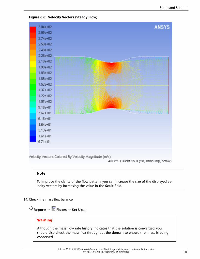
Figure 6.6: Velocity Vectors (Steady Flow)
Note
To improve the clarity of the flow pattern, you can increase the size of the displayed ve-
locity vectors by increasing the value in the Scale field.
14. Check the mass flux balance.
Reports → Fluxes → Set Up...
Warning
Although the mass flow rate history indicates that the solution is converged, you
should also check the mass flux throughout the domain to ensure that mass is being
conserved.
281Release 15.0 - © SAS IP, Inc. All rights reserved. - Contains proprietary and confidential information
of ANSYS, Inc. and its subsidiaries and affiliates.
Setup and Solution

a. Retain the default selection of Mass Flow Rate.
b. Select inlet and outlet in the Boundaries selection list.
c. Click Compute and examine the values displayed in the dialog box.
Warning
The net mass imbalance should be a small fraction (for example, 0.1%) of the
total flux through the system. The imbalance is displayed in the lower right field
under Net Results. If a significant imbalance occurs, you should decrease your
residual tolerances by at least an order of magnitude and continue iterating.
d. Close the Flux Reports dialog box.
6.4.9. Enabling Time Dependence and Setting Transient Conditions
In this step you will define a transient flow by specifying a transient pressure condition for the nozzle.
1. Enable a time-dependent flow calculation.
General
Release 15.0 - © SAS IP, Inc. All rights reserved. - Contains proprietary and confidential informationof ANSYS, Inc. and its subsidiaries and affiliates.282
Modeling Transient Compressible Flow

a. Select Transient in the Time list.
2. Read the user-defined function (�������), in preparation for defining the transient condition for the
nozzle exit.
Define → User-Defined → Functions → Interpreted...
The pressure at the outlet is defined as a wave-shaped profile, and is described by the following equation:
(6.1)� �
where
circular frequency of transient pressure
(rad/s)
=
mean exit pressure (atm)=
In this case, � rad/s, and � atm.
A user-defined function (�������) has been written to define the equation (Equation 6.1 (p. 283)) required
for the pressure profile.
Note
To input the value of Equation 6.1 (p. 283) in the correct units, the function ������� has
to be written in SI units.
More details about user-defined functions can be found in the UDF Manual.
283Release 15.0 - © SAS IP, Inc. All rights reserved. - Contains proprietary and confidential information
of ANSYS, Inc. and its subsidiaries and affiliates.
Setup and Solution

a. Enter ������� for Source File Name.
If the UDF source file is not in your working directory, then you must enter the entire directory path
for Source File Name instead of just entering the file name.
b. Click Interpret.
The user-defined function has already been defined, but it must be compiled within ANSYS Fluent before
it can be used in the solver.
c. Close the Interpreted UDFs dialog box.
3. Set the transient boundary conditions at the nozzle exit (outlet).
Boundary Conditions → outlet → Edit...
Release 15.0 - © SAS IP, Inc. All rights reserved. - Contains proprietary and confidential informationof ANSYS, Inc. and its subsidiaries and affiliates.284
Modeling Transient Compressible Flow

a. Select udf transient_pressure (the user-defined function) from the Gauge Pressure drop-down list.
b. Click OK to close the Pressure Outlet dialog box.
4. Update the gradient adaption parameters for the transient case.
Adapt → Gradient...
a. Enter �� for Interval in the Dynamic group box.
For the transient case, the mesh adaption will be done every 10 time steps.
b. Enter ��� for Coarsen Threshold.
c. Enter ��� for Refine Threshold.
The refine and coarsen thresholds have been changed during the steady-state computation to meet
the limit of 20000 cells. Therefore, you must reset these parameters to their original values.
d. Click Apply to store the values.
e. Click Controls... to open the Mesh Adaption Controls dialog box.
i. Enter ���� for Min # of Cells.
ii. Enter ����� for Max # of Cells.
You must increase the maximum number of cells to try to avoid readjustment of the coarsen and
refine thresholds. Additionally, you must limit the minimum number of cells to 8000, because you
should not have a coarse mesh during the computation (the current mesh has approximately
20000 cells).
iii. Click OK to close the Mesh Adaption Controls dialog box.
f. Close the Gradient Adaption dialog box.
6.4.10. Specifying Solution Parameters for Transient Flow and Solving
1. Modify the plotting of the mass flow rate at the nozzle exit.
Monitors (Surface Monitors) → surf-mon-1 → Edit...
Because each time step requires 10 iterations, a smoother plot will be generated by plotting at every time
step.
285Release 15.0 - © SAS IP, Inc. All rights reserved. - Contains proprietary and confidential information
of ANSYS, Inc. and its subsidiaries and affiliates.
Setup and Solution

a. Set Window to 3.
b. Enter ����������� for File Name.
c. Select Time Step from the X Axis drop-down list.
d. Select Time Step from the Get Data Every drop-down list.
e. Click OK to close the Surface Monitor dialog box.
2. Save the transient solution case file (��������������).
File → Write → Case...
3. Modify the plotting of residuals.
Monitors → Residuals → Edit...
a. Ensure that Plot is enabled in the Options group box.
b. Ensure none is selected from the Convergence Criterion drop-down list.
c. Set the Iterations to Plot to ���.
d. Click OK to close the Residual Monitors dialog box.
4. Set the time step parameters.
Release 15.0 - © SAS IP, Inc. All rights reserved. - Contains proprietary and confidential informationof ANSYS, Inc. and its subsidiaries and affiliates.286
Modeling Transient Compressible Flow

Run Calculation
The selection of the time step is critical for accurate time-dependent flow predictions. Using a time step
of 2.85596x10⁻⁵
seconds, 100 time steps are required for one pressure cycle. The pressure cycle begins
and ends with the initial pressure at the nozzle exit.
a. Enter ���������� s for Time Step Size.
b. Enter ��� for Number of Time Steps.
c. Enter �� for Max Iterations/Time Step.
d. Click Calculate to start the transient simulation.
Warning
Calculating 600 time steps will require significant CPU resources. Instead of calculating
the solution, you can read the data file (��������������) with the precalculated
solution. This data file can be found in the folder where you found the mesh and
UDF files.
287Release 15.0 - © SAS IP, Inc. All rights reserved. - Contains proprietary and confidential information
of ANSYS, Inc. and its subsidiaries and affiliates.
Setup and Solution

By requesting 600 time steps, you are asking ANSYS Fluent to compute six pressure cycles. The mass flow
rate history is shown in Figure 6.7: Mass Flow Rate History (Transient Flow) (p. 288).
Figure 6.7: Mass Flow Rate History (Transient Flow)
5. Optionally, you can review the effect of dynamic mesh adaption performed during transient flow com-
putation as you did in steady-state flow case.
6. Save the transient case and data files (�������������� and ��������������).
File → Write → Case & Data...
6.4.11. Saving and Postprocessing Time-Dependent Data Sets
At this point, the solution has reached a time-periodic state. To study how the flow changes within a single
pressure cycle, you will now continue the solution for 100 more time steps. You will use ANSYS Fluent’s
solution animation feature to save contour plots of pressure and Mach number at each time step, and the
autosave feature to save case and data files every 10 time steps. After the calculation is complete, you will
use the solution animation playback feature to view the animated pressure and Mach number plots over
time.
1. Request the saving of case and data files every 10 time steps.
Calculation Activities (Autosave Every) → Edit...
Release 15.0 - © SAS IP, Inc. All rights reserved. - Contains proprietary and confidential informationof ANSYS, Inc. and its subsidiaries and affiliates.288
Modeling Transient Compressible Flow

a. Enter �� for Save Data File Every.
b. Select Each Time for Save Associated Case Files.
c. Retain the default selection of time-step from the Append File Name with drop-down list.
d. Enter �������� for File Name.
When ANSYS Fluent saves a file, it will append the time step value to the file name prefix (��������).
The standard extensions (���� and ����) will also be appended. This will yield file names of the
form �������������������� and ��������������������, where ����� is the time step
number.
Optionally, you can add the extension ��� to the end of the file name (for example, �����������),
which will instruct ANSYS Fluent to save the case and data files in compressed format, yielding file
names of the form �����������������������.
e. Click OK to close the Autosave dialog box.
Extra
If you have constraints on disk space, you can restrict the number of files saved by
ANSYS Fluent by enabling the Retain Only the Most Recent Files option and setting
the Maximum Number of Data Files to a nonzero number.
2. Create animation sequences for the nozzle pressure and Mach number contour plots.
Calculation Activities (Solution Animations) → Create/Edit...
289Release 15.0 - © SAS IP, Inc. All rights reserved. - Contains proprietary and confidential information
of ANSYS, Inc. and its subsidiaries and affiliates.
Setup and Solution

a. Set Animation Sequences to �.
b. Enter �������� for the Name of the first sequence and ����������� for the second sequence.
c. Select Time Step from the When drop-down lists for both sequences.
The default value of � in the Every integer number entry box instructs ANSYS Fluent to update the
animation sequence at every time step.
d. Click the Define... button for pressure to open the associated Animation Sequence dialog box.
i. Select In Memory from the Storage Type group box.
The In Memory option is acceptable for a small 2D case such as this. For larger 2D or 3D cases,
saving animation files with either the Metafile or PPM Image option is preferable, to avoid using
too much of your machine’s memory.
ii. Enter � for Window and click the Set button.
Release 15.0 - © SAS IP, Inc. All rights reserved. - Contains proprietary and confidential informationof ANSYS, Inc. and its subsidiaries and affiliates.290
Modeling Transient Compressible Flow

iii. Select Contours from the Display Type group box to open the Contours dialog box.
A. Ensure that Filled is enabled in the Options group box.
B. Disable Auto Range.
C. Retain the default selection of Pressure... and Static Pressure from the Contours of drop-
down lists.
D. Enter ���� atm for Min and ���� atm for Max.
This will set a fixed range for the contour plot and subsequent animation.
E. Click Display and close the Contours dialog box.
Figure 6.8: Pressure Contours at t=0.017136 s (p. 292) shows the contours of static pressure in
the nozzle after 600 time steps.
291Release 15.0 - © SAS IP, Inc. All rights reserved. - Contains proprietary and confidential information
of ANSYS, Inc. and its subsidiaries and affiliates.
Setup and Solution
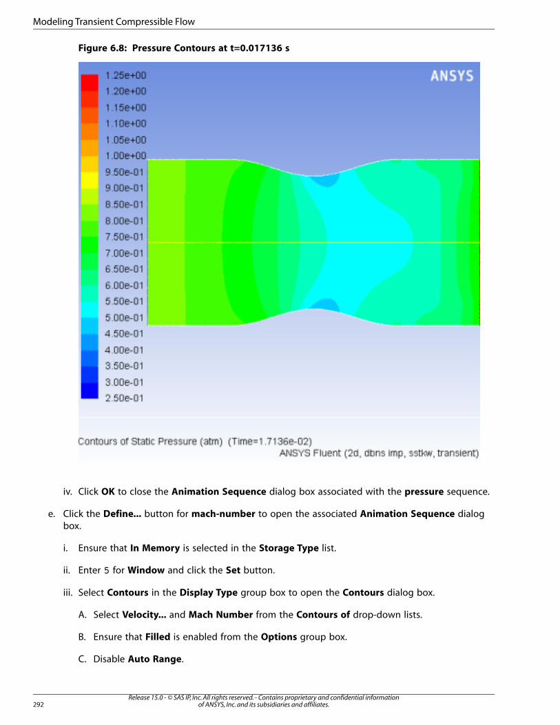
Figure 6.8: Pressure Contours at t=0.017136 s
iv. Click OK to close the Animation Sequence dialog box associated with the pressure sequence.
e. Click the Define... button for mach-number to open the associated Animation Sequence dialog
box.
i. Ensure that In Memory is selected in the Storage Type list.
ii. Enter � for Window and click the Set button.
iii. Select Contours in the Display Type group box to open the Contours dialog box.
A. Select Velocity... and Mach Number from the Contours of drop-down lists.
B. Ensure that Filled is enabled from the Options group box.
C. Disable Auto Range.
Release 15.0 - © SAS IP, Inc. All rights reserved. - Contains proprietary and confidential informationof ANSYS, Inc. and its subsidiaries and affiliates.292
Modeling Transient Compressible Flow

D. Enter ���� for Min and ���� for Max.
E. Click Display and close the Contours dialog box.
Figure 6.9: Mach Number Contours at t=0.017136 s (p. 293) shows the Mach number contours
in the nozzle after 600 time steps.
Figure 6.9: Mach Number Contours at t=0.017136 s
iv. Click OK to close the Animation Sequence dialog box associated with the mach-number sequence.
f. Click OK to close the Solution Animation dialog box.
3. Continue the calculation by requesting 100 time steps.
Run Calculation
293Release 15.0 - © SAS IP, Inc. All rights reserved. - Contains proprietary and confidential information
of ANSYS, Inc. and its subsidiaries and affiliates.
Setup and Solution

By requesting 100 time steps, you will march the solution through an additional 0.0028 seconds, or
roughly one pressure cycle.
With the autosave and animation features active (as defined previously), the case and data files will be
saved approximately every 0.00028 seconds of the solution time; animation files will be saved every
0.000028 seconds of the solution time.
Enter ��� for Number of Time Steps and click Calculate.
When the calculation finishes, you will have ten pairs of case and data files and there will be 100 pairs
of contour plots stored in memory. In the next few steps, you will play back the animation sequences
and examine the results at several time steps after reading in pairs of newly saved case and data files.
4. Change the display options to include double buffering.
Graphics and Animations → Options...
Double buffering will allow for a smoother transition between the frames of the animations.
Release 15.0 - © SAS IP, Inc. All rights reserved. - Contains proprietary and confidential informationof ANSYS, Inc. and its subsidiaries and affiliates.294
Modeling Transient Compressible Flow

a. Retain the Double Buffering option in the Rendering group box.
b. Enter � for Active Window and click the Set button.
Note
Alternatively, you can change the active window using the drop-down list at the top
of the graphics window.
c. Click Apply and close the Display Options dialog box.
5. Play the animation of the pressure contours.
Graphics and Animations → Solution Animation Playback → Set Up...
295Release 15.0 - © SAS IP, Inc. All rights reserved. - Contains proprietary and confidential information
of ANSYS, Inc. and its subsidiaries and affiliates.
Setup and Solution

a. Retain the default selection of pressure in the Sequences selection list.
Ensure that window 4 is visible in the viewer. If it is not, select it from the drop-down list at the
top left of the viewer window.
b. Click the play button (the second from the right in the group of buttons in the Playback group box).
c. Close the Playback dialog box.
Examples of pressure contours at � s (the 630th time step) and � s (the 670th
time step) are shown in Figure 6.10: Pressure Contours at t=0.017993 s (p. 297) and Figure 6.11: Pressure
Contours at t=0.019135 s (p. 298).
6. In a similar manner to steps 4 and 5, select the appropriate active window and sequence name for the
Mach number contours.
Examples of Mach number contours at � s and � s are shown in Figure 6.12: Mach
Number Contours at t=0.017993 s (p. 299) and Figure 6.13: Mach Number Contours at t=0.019135 s (p. 300)..
Release 15.0 - © SAS IP, Inc. All rights reserved. - Contains proprietary and confidential informationof ANSYS, Inc. and its subsidiaries and affiliates.296
Modeling Transient Compressible Flow

Figure 6.10: Pressure Contours at t=0.017993 s
297Release 15.0 - © SAS IP, Inc. All rights reserved. - Contains proprietary and confidential information
of ANSYS, Inc. and its subsidiaries and affiliates.
Setup and Solution

Figure 6.11: Pressure Contours at t=0.019135 s
Release 15.0 - © SAS IP, Inc. All rights reserved. - Contains proprietary and confidential informationof ANSYS, Inc. and its subsidiaries and affiliates.298
Modeling Transient Compressible Flow
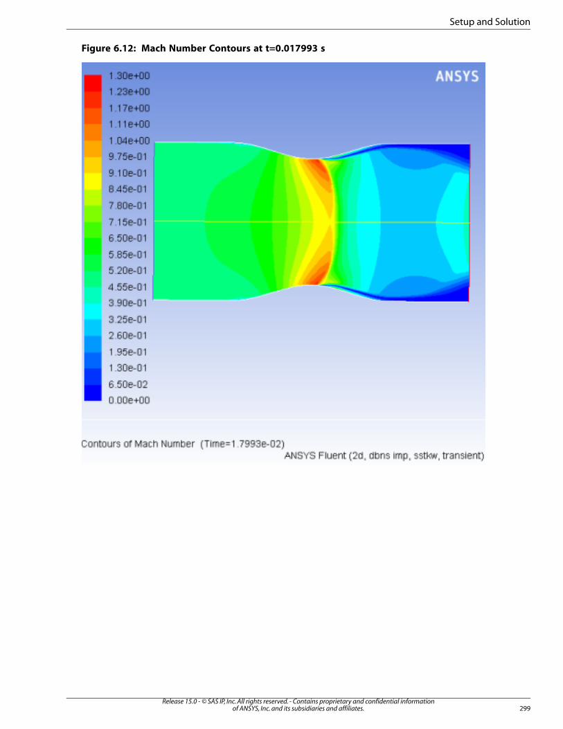
Figure 6.12: Mach Number Contours at t=0.017993 s
299Release 15.0 - © SAS IP, Inc. All rights reserved. - Contains proprietary and confidential information
of ANSYS, Inc. and its subsidiaries and affiliates.
Setup and Solution
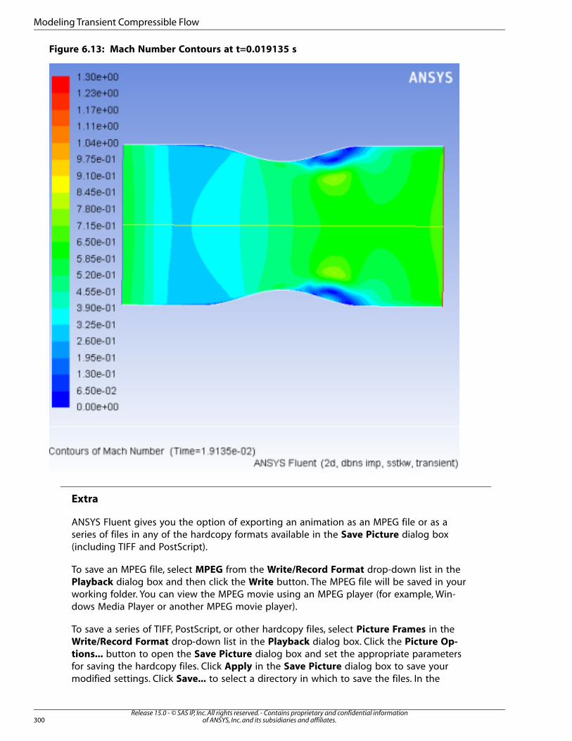
Figure 6.13: Mach Number Contours at t=0.019135 s
Extra
ANSYS Fluent gives you the option of exporting an animation as an MPEG file or as a
series of files in any of the hardcopy formats available in the Save Picture dialog box
(including TIFF and PostScript).
To save an MPEG file, select MPEG from the Write/Record Format drop-down list in the
Playback dialog box and then click the Write button. The MPEG file will be saved in your
working folder. You can view the MPEG movie using an MPEG player (for example, Win-
dows Media Player or another MPEG movie player).
To save a series of TIFF, PostScript, or other hardcopy files, select Picture Frames in the
Write/Record Format drop-down list in the Playback dialog box. Click the Picture Op-tions... button to open the Save Picture dialog box and set the appropriate parameters
for saving the hardcopy files. Click Apply in the Save Picture dialog box to save your
modified settings. Click Save... to select a directory in which to save the files. In the
Release 15.0 - © SAS IP, Inc. All rights reserved. - Contains proprietary and confidential informationof ANSYS, Inc. and its subsidiaries and affiliates.300
Modeling Transient Compressible Flow

Playback dialog box, click the Write button. ANSYS Fluent will replay the animation,
saving each frame to a separate file in your working folder.
If you want to view the solution animation in a later ANSYS Fluent session, you can select
Animation Frames as the Write/Record Format and click Write.
Warning
Since the solution animation was stored in memory, it will be lost if you exit ANSYS
Fluent without saving it in one of the formats described previously. Note that only
the animation-frame format can be read back into the Playback dialog box for display
in a later ANSYS Fluent session.
7. Read the case and data files for the 660th time step (noz_anim–1–00660.cas.gz and noz_an-im–1–00660.dat.gz) into ANSYS Fluent.
8. Plot vectors at � s (Figure 6.14: Velocity Vectors at t=0.018849 s (p. 302)).
Graphics and Animations → Vectors → Set Up...
a. Ensure Auto Scale is enabled under Options.
b. Retain the default values for all other properties.
301Release 15.0 - © SAS IP, Inc. All rights reserved. - Contains proprietary and confidential information
of ANSYS, Inc. and its subsidiaries and affiliates.
Setup and Solution
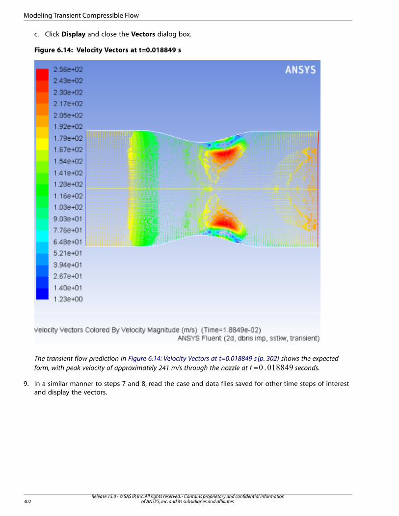
c. Click Display and close the Vectors dialog box.
Figure 6.14: Velocity Vectors at t=0.018849 s
The transient flow prediction in Figure 6.14: Velocity Vectors at t=0.018849 s (p. 302) shows the expected
form, with peak velocity of approximately 241 m/s through the nozzle at � seconds.
9. In a similar manner to steps 7 and 8, read the case and data files saved for other time steps of interest
and display the vectors.
6.5. Summary
In this tutorial, you modeled the transient flow of air through a nozzle. You learned how to generate a
steady-state solution as an initial condition for the transient case, and how to set solution parameters
for implicit time-stepping.
You also learned how to manage the file saving and graphical postprocessing for time-dependent flows,
using file autosaving to automatically save solution information as the transient calculation proceeds.
Release 15.0 - © SAS IP, Inc. All rights reserved. - Contains proprietary and confidential informationof ANSYS, Inc. and its subsidiaries and affiliates.302
Modeling Transient Compressible Flow

Finally, you learned how to use ANSYS Fluent’s solution animation tool to create animations of transient
data, and how to view the animations using the playback feature.
6.6. Further Improvements
This tutorial guides you through the steps to generate a second-order solution. You may be able to
increase the accuracy of the solution even further by using an appropriate higher-order discretization
scheme and by adapting the mesh further. Mesh adaption can also ensure that the solution is independ-
ent of the mesh. These steps are demonstrated in Introduction to Using ANSYS Fluent: Fluid Flow and
Heat Transfer in a Mixing Elbow (p. 123).
303Release 15.0 - © SAS IP, Inc. All rights reserved. - Contains proprietary and confidential information
of ANSYS, Inc. and its subsidiaries and affiliates.
Further Improvements


![Aerodynamic and Static Aeroelastic Analysis of a Transonic ...iieng.org/images/proceedings_pdf/8773E1214053.pdfastronautics. HUNS3D flow solver [6], [7] designed for both 2D and 3D](https://img.dokumen.tips/doc/110x75/5f85984f6a43ca5909311125/aerodynamic-and-static-aeroelastic-analysis-of-a-transonic-iiengorgimagesproceedingspdf.jpg)


