Final Report

Discontinuous Galerkin Compressible Euler Equation Solver

May 14, 2013

Andrey Andreyev

Adviser: Dr. James Baeder

Abstract:

In this work a Discontinuous Galerkin Method is developed for compressible Euler Equations. This method seeks to project the exact solution onto a finite polynomial space while allowing for discontinuities at cell interfaces. This allows for the natural discontinuity capture that is required for a compressible flow solver. The appeal of the Discontinuous Galerkin Method is that it handles higher order spatial discretization without the use of larger stencils which is required in Finite Volume/Difference implementations. Spatial discretization order is increased by adding degrees of freedom to a cell. This also has the added advantage of an easily controllable order of accuracy in areas of interest.

The Discontinuous Galerkin Method is then applied to one and two dimensional Euler Equation problems to test its ability to solve smooth and discontinuous problems. The smooth problems, which have an analytical solution, were used to test the method’s accuracy while the discontinuous problems were used to test the method’s shock capturing ability. The use of a TVD limiter was required for discontinuous problems. All problems were tested using a second and third order spatial discretization. To test the formal order of the method a grid refinement study was performed using the smooth solutions. The second order spatial discretization proved to 2nd order for one and two dimensional problems. While the third order spatial discretization proved to be slightly worse than 3rd order; however it also proved to be less diffusive which a desired property in a numerical scheme. The TVD limiter was tested using problems which are known to have discontinuous solutions, although analytical solutions do not exist, except for Sod’s Shock tube problem in one dimension. The TVD limiter was found to be diffusive and needed extra limiting around very strong discontinuities. The solution to this issue is the subject of current work.

List of Symbols Relevant to Discontinuous Galerkin Formulation …………………………………………………State Vector of Conserved Quantities in the Euler Equation ………………………………..Flux Vector in two dimensions

............................................Flux at the cell interface

……………………………………Approximate solution to within each cell

…………………………………………Finite Element Degrees of freedom

……………………………………………..Finite Element Shape Functions

………………………………………………Finite Element Weight Functions (same as shape functions)

]……………………………………………..Mass Matrix resulting from finite element derivations

………………………………………………..Degree of freedom indicator

…………………………………………………Flux Jacobian

…………………………………………………..Natural Coordinate within the cell [-1,1] in x direction η …………………………………………………..Natural Coordinate within the cell [-1,1] in y direction

1 Introduction: The need to solve inviscid, compressible flow governed by the Euler Equations comprises a large set of engineering problems of practical importance. Unfortunately the Euler Equations are a system of non-linear partial differential equations which have few exact solutions. The exact solutions that do exist are based on a series of simplifying assumptions that make the solutions not applicable to engineering problems. The need of robust numerical methods to solve the Euler Equations is of great importance.

Traditionally finite difference and finite volume methods are used in development of compressible flow solvers with finite volume method being dominant because of its natural conservative properties [3]. However these methods are difficult to make higher order in space because of the need for a larger stencil size to approximate the gradients numerically. The details of this will be discussed in further detail in the mathematical background section. The appeal of the Discontinuous Galerkin method is that in finite element formulations gradients of the approximate solution are represented as shape functions and thus there is no need to use a larger computational stencil. This has several implications. The first being is that boundary treatment is simpler because there is no need to adjust the computational stencil around domain boundaries. The second implication is that there is less “numerical smearing” around flow discontinuities because the numerical gradients are not calculated based on several values across the discontinuity. This feature is known as locality [2].

1.1 Mathematical Background of Euler Equations Euler Equations are a system of Hyperbolic Partial Differential Equations (PDEs). Euler equations can be expressed in several forms. However the form that is of interest in compressible fluid dynamics is conservation form, which uses conservative variables. This form allows for continuous fluxes across discontinuities [5]. The three dimensional form of the Euler Equations in conservative form is shown in equation 1.1.1 [1].

(1.1.1)

In equation 1.1.1 is the density, is the velocity in the x direction, is the velocity in the y direction, is the velocity in z direction, is the pressure, is the ration of specific heats, and is the energy. The vector is the vector of conservative variables which consists of the primary variables . Almost all compressible codes seek to find the solution in space and time. The vectors are the flux vectors in the x, y, and z direction respectively [1]. Equation 1.1.1 only has analytical for a specific set of simplified problems and generally the solution is obtained numerically. Numerical methods usually discretize the spatial domain using a computational grid and the Euler Equations are solved approximately within each cell of the grid to obtain a global solution at a given time. A numerical method that is capable of naturally capturing the discontinuities in the solution is called a conservative method [3].

1.2 Conservative Numerical Scheme Overview One major characteristic of hyperbolic equations such as the Euler Equations is that it allows for discontinuities in the solution and the ability of numerical methods to handle the discontinuities automatically as part of the solution procedure is a desired property. Figure 1 shows the difference between a conservative and non-conservative method solution in one dimension [3].

Figure 1 Difference Between conservative and non-conservative methods [3]

Finite Volume and Finite Difference methods use stencils to approximate the derivates of the Euler Equations. Stencils are locations where functions are sampled to provide to provide information of the behavior of the solution. Generally the larger the stencil, the more accurate the approximation becomes. A graphical representation of a numerical stencil is shown in figure 2 [3]. The stencil presented is for a one dimensional problem. The horizontal axis is the spatial variable discretization and the vertical axis is the time.

Figure 2 Graphical Representation of a computational stencil [3]

As one can imagine, if there is a discontinuity within the stencil, the result for the derivative will be polluted. One can also see the boundary treatment implications. Imagine a boundary on the right side of the horizontal axis, the derivative approximation near that boundary will be problematic once points to the right of the boundary are required.

A finite element implementation seeks to avoid this issue of larger stencils by using higher order shape functions to approximate the variation (derivative) of the solution. The reason why finite element methods were not used for Euler Equations solvers is that traditional methods were not conservative because they enforced discontinuities across cell interfaces. It is the Discontinuous Galerkin Method that allows for discontinuities across cell interfaces and thus allows discontinuous solutions [1].

2 Project Objectives

The goal of this project was to develop a Discontinuous Galerkin inviscid flow solver capable of capturing

shocks in the solution. The flow solver was developed in one and two dimensions and designed to be up

to 3rd order accurate in space and time. The project was divided in to two sections. One section

dedicated to developing the one dimensional code, and the other to developing the two dimensional

code. All coding was done using Fortran 90/95.

For each, the one dimensional and the two dimensional code, a set of test problems were used to

validate the solutions obtained as well as to test the shock capturing properties of the solvers. To

validate the one dimensional solver, an entropy wave convection problem was used. This problem was

chosen because it has an analytical solution and the solution is smooth thus it does not require the use

of a TVD limiter.

To validate the one dimensional code, the observed spatial accuracy was calculated using a grid

refinement study. This is done by sequentially doubling the amount of cells used and observing the

behavior of the error norms. Once this was completed, two problems with strong discontinuities were

used to test the codes ability to capture shocks. The first problem was Sod’s Shock Tube problem which

has a known solution. The second problem was Osher’s problem which tests, not only the shock

capturing properties, but the schemes ability to resolve small scale flow features. This problem does not

have an exact solution and the accuracy was tested visually by looking for known flow features within

the solution.

As in the one dimensional case, a grid refinement study was performed to validate the two dimensional

code. The problem chosen was the isentropic vortex problem which is the two dimensional analog to

the entropy wave problem in one dimension. The reason for choosing this problem is the same as the

entropy wave. To test the shock capturing abilities of the code, a Double Mach Reflection problem was

used. This was chosen because the solution has a very strong shock, and although it does not have an

exact solution, there is a lot of literature with the results for this problem. The accuracy of the solution

was judged based on observations from literature.

3. Development of Discontinuous Galerkin Method

As any finite element method, the Discontinuous Galerkin (DG) Method seeks to project the solution

onto a finite polynomial function space . The order of the polynomial space is what determines the spatial order of the method [1]. What separates the DG method from other finite element methods is that it does not enforce continuity across cells which allows for discontinuous solutions. A general development of the DG method is outlined in this section. The simplification to a one and two dimensional scheme will be developed in the following subsections.

As mentioned earlier, the domain is discretized into N cells. Consider the Euler Equation 1.1.1 which must hold at each cell . The approximate solution to is defined as equation 3.1.

(3.1)

are the degrees of freedom to be determined and

are the polynomial space functions.

is the order of the polynomial space and defines the order of the spatial discretization. For example, when the method is second order. Note that the bold symbols are the state vectors where as the symbols with arrows over them are the spatial vectors. Also the details of the degrees of freedom and the shape functions are intentionally left vague because the finite element method can be formally derived with any number of combinations of degrees of freedom and shape functions [1]. The details of these will be given when deriving the specific one and two dimensional cases. Equation 3.1 is substituted into equation 1.1.1, multiplied by a weight function and integrated over the volume of the cell. The choice of a weight function defines the type of finite element method. If the weight functions are chosen to be the same as the shape function, the method is known as the Galerkin Method [1].

(3.2)

Equation 3.2 is then integrated by parts to obtain the weak form of the equation [6].

(3.3)

Note that equation 3.3 is a system of ordinary differential equations (ODE) in time for the degrees of

freedom. In this case is the complete flux vector with the x, y, and z components and is the local

mass matrix. If this were the development of a traditional continuous finite element method, the derivation would be complete. Local system would be assembled into a global system using the assumption that the terms in 1st term of the RHS are continuous. These terms are known as the boundary terms. However in the DG method there are no assumption on the continuity of the boundary terms, thus the system is ill defined unless the fluxes at the boundary are defined [6]. The surface and volume integrals are usually carried out numerically using Gauss quadrature [4]. The boundary fluxes can be defined in many ways, but all are based on the solution to the Riemann problem at the cell interface. The Riemann problem is defined as

(3.4)

Equation 3.4 has an analytical solution for the Euler Equations and can be found in [3]. However it too expensive to solve at each cell interface, thus approximate Riemann solvers are usually used. There are many approximate Riemann solvers and they can be found in [6]. This work incorporated the Roe Approximate Riemann solver [6]. Once the boundary fluxes are defined, the derivation of the DG method is complete. Note that since there are no requirements on the continuity of solution, each cell has a local mass matrix which can be inverted a priori thus eliminating the need for a system solver [1]. Since the RHS of equation 3.3 is defined, each cell can be integrated in time for the degrees of freedom using any explicit time integrator. In this work a three stage Runge-Kutta was used to march in time [2].

(3.5)

is the right hand side of equation 3.3 and When discontinuities are present a TVD projection limiter has to be applied at each Runge-Kutta time step. The details of the projection limiter will be explained in the following subsections when applied to one and two dimensional cases. 3.1 One Dimensional Discontinuous Galerkin Method

The one dimensional version of the DG method uses Legendre polynomials as the shape and weight functions.

(3.1.1a)

(3.1.1b)

(2.1.1.c)

(3.1.2)

is the cell center. Note that when Legendre polynomials are used as the shape and weight functions,

the mass matrix is diagonal with entries being

. Using equations 3.1.1 and 3.1.2 and applying them to

the general weak form (equation 2.3) the following is obtained [2].

(3.1.3)

Equation 3.1.3 uses an operator which is a positive difference operator on quantity ,

.

As mentioned in the previous section the interface flux or the boundary flux is calculated using an

approximate Riemann solver. In this case a one dimensional Roe Flux was used to solve [3].

3.1.4)

defines the change of a quantity across the interface.

In order to calculate the fluxes at the cell interface, the values of are required. They are

calculated using equation 3.1.1a. However, for any scheme higher than 1st order, these quantities need

to be limited to guarantee stability. For this, a limiter is required. A limiter guarantees the degrees of

freedom that account for variation of the cell are not large enough to cause instability. There are

various choices for a limiter used in literature (mostly for finite volume/difference scheme). The minmod

limiter was used in this work and is described below [1].

The evaluation of at the interface is obtained by evaluating (3.1.1a) at the each interface. After

some manipulation

where

are the degrees of freedom. Note that the above equation is for a third order scheme. To

obtain second order scheme, the third term is dropped in each equation. The above quantities need to

be limited in the characteristic variables. To do this, a flux Jacobian,

, is calculated. By the following

procedure [2].

Compute and calculate the Flux Jacobian

at . Calculate the matrices

which consist of right eigenvectors as columns and left eigenvectors as rows respectively. [3]

Calculate

and

multiply each by to project each of the variables onto the left eigenspace.

where represents all of the above variables. The goal is to limit in the left

eigenspace by applying the minmod limiter. A minmod function

returns the lowest value unless there is a sign difference in in which case it

returns zero [1].

)

(3.1.5)

The modified values are now used to project

onto the cell interface

and project back on to component space by

This result is used in the Roe Flux function shown earlier.

The only step left is to march in time using the third order Runge-Kutta Technique given by equation 2.5

[1].

This completes the development of the 1D Discontinuous Galerkin Method. The 2D version is given in

the next subsection.

3.2 Two Dimensional Discontinuous Galerkin Method

The development of the two-dimensional DG method follows the same procedure as the one-

dimensional DG method. The degrees of freedom and the shape functions need to be defined.

The shape functions are defined as Legendre polynomials which use natural coordinates from -1 to 1.

is used as the natural coordinate in x and is used as the natural coordinate in y. The shape functions at

cell are given by equation 3.2.1

(3.2.1)

Note that the functions which have subscript refer to the function number, and not a power.

The approximate solution defined up to 3rd order is given by 3.2.2

(3.2.2)

To make the method 2nd order, the last three terms are removed.

The weak form is given by equation 2.3

(3.2.3)

For this choice of shape functions and degrees of freedom, is a diagonal matrix with the following

entries.

Note that

is replaced by

and

, but the concept remains the same. Also note that the

boundary term now requires a surface integral around the cell interface. The boundary term is

computed using a two dimensional approximate Roe solver analogous to the one used in the one

dimensional case. Since two dimensional approximate Riemann solvers are lengthy, the reader is

referred to [7] for the formula of the 2D Roe Solver used in this work.

The second integral on RHS of 3.3 is a double integral and evaluated using 2D quadrature which is a

tensor product of 1D quadrature rule.

(3.2.3)

The above formulation fully defines the spatial discretization of the two dimensional scheme. Just as in

the one dimensional scheme, all that is left is apply the TVD minmod limiter to the interface values and

march in time using the 3rd order Runge-Kutta.

Just as in the one dimensional case, a TVD minmod limiter is added to the time marching to stabilize the

scheme when discontinuities are present. The only difference between the minmod limiter in two

dimensions is that it has to be applied twice: once for variation of in x and once for variation in y. Also

if the cell is flagged to be limited, the third order terms are removed. This is justified by the fact that if

the solution is being limited, there is no guarantee that the third order degrees of freedom are accurate

[6].

Again equation 3.3 is integrated in time for the degrees of freedom using the third order Runge-Kutta

[5].

4 Validation and Results

In this section the test problems for the one and two dimensional cases are presented. The smooth

solutions are used as the validation cases whereas the discontinuous solutions are used to test the

scheme’s ability to capture the discontinuities in the solution.

4.1 One Dimensional Validation and Results

The sections below describe the validation procedure for the one dimensional code. Again, the smooth

solution used for validation is the entropy wave convection and the discontinuous solutions used to test

shock capturing capabilities and by extension, the TVD limiter are Sod’s Shock Tube problem and Osher’s

Problem.

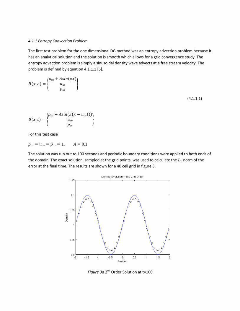
4.1.1 Entropy Convection Problem

The first test problem for the one dimensional DG method was an entropy advection problem because it

has an analytical solution and the solution is smooth which allows for a grid convergence study. The

entropy advection problem is simply a sinusoidal density wave advects at a free stream velocity. The

problem is defined by equation 4.1.1.1 [5].

(4.1.1.1)

For this test case

The solution was run out to 100 seconds and periodic boundary conditions were applied to both ends of

the domain. The exact solution, sampled at the grid points, was used to calculate the norm of the

error at the final time. The results are shown for a 40 cell grid in figure 3.

Figure 3a 2nd Order Solution at t=100

Figure 3b 3rd Order Solution at t=100

From visual inspection it can be seen that the 3rd order method is less dissipative than the 2nd order

method. This is the desired result since increase in spatial accuracy is motivated by the reduction is

numerical dissipation.

In order to test the formal order of the scheme a grid refinement study was performed by doubling the

number of cells and observing the of the error. Five grid sizes were used [10, 20, 40, 80, 160]. The

error vs. the number of cells is plotted in figure 4.

Figure 4 LogLog Plot of the Error

Figure 4 shows how the error behaves as the grid is refined. The slope of the line gives the observed

order of accuracy. The slope of the 2nd order line is 2.26 and the slope of the 3rd order line is 3.67, which

implies that the second order scheme is super convergent. This result proves that the code provides

satisfactory results for smooth solutions.

4.1.2 Sod’s Shock Tube Problem

To test the shock capturing abilities of the scheme Sod’s shock tube problem and Osher’s problem were

used as the test cases.

Sod’s shock tube problem is simple shock tube which is simply a Riemann problem which has an

analytical solution. However due to the flat nature of the solution, error estimates do not provide much

useful information. The left and right states of the Riemann problem are defined as

= 0.1, 0.0, 0.125

For both schemes 100 cells were used and the solution was run out to 2.0 seconds. Zero Gradient

boundary condition was applied.

The density results along with the exact solution are shown in figure 5.

Figure 5a Density 2nd Order N=100

Figure 5b Density 3rd Order N=100

Figure 5 shows that both the schemes are capable of capturing the discontinuities in the solution with

minimal oscillatory behavior. In fact the 3rd order scheme has smoother transitions between

discontinuities.

4.1.3 Osher’s Problem

An entropy and shock wave interaction was also used as a test case. This is known as the Osher problem

and was taken out of [1]. This problem tests the shock capturing as well as the ability to resolve

complicated flow features [5]. The initial condition is given by 4.1.3.1. The figures for the results are

shown below. The method was able to capture the n-wave patterns as well as the features circled in 4.

The third order method is shown to be less diffusive and is able to capture the flow features better.

(4.1.3.1)

The problem was run using 200 cells for both schemes and run out to 1.8 seconds. Zero gradient

boundary conditions were applied to both ends of the domain. The results were then plotted and

compared to the calculated solution from literature which is defined as the accurate solution.[4].

*-

Figure 6a. Calculated Solution to the Osher Problem[4]

Figure 6b 2nd Order Solution N=200

Figure 6b 3rd Order Solution N=200

Comparing the above figures, the 3rd order method matches more closes with the verified calculated

solution.

4.2 Two Dimensional Validation and Results

The sections below describe the validation procedure for the two dimensional code. The smooth

solution used for validation is the isentropic vortex convection and the discontinuous solution used to

test shock capturing capabilities and by extension, the TVD limiter is the Double Mach Reflection

Problem.

4.2.1 Isentropic Vortex Convection

The first test problem for the two dimensional case was the isentropic vortex convection problem. This

problem has an analytical smooth solution which can be subjected to a grid convergence study. Also

because the solution is smooth, the possibility of the TVD limiter corrupting the solution. The isentropic

vortex convection problem is the analog to the entropy wave in one dimension. The initial vortex should

convect at the free stream velocity. The problem is defined by 4.2.1 [5]

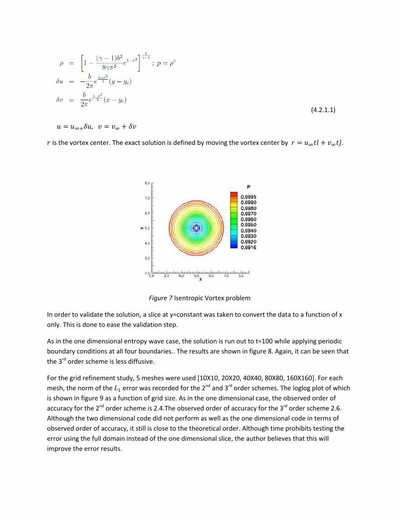
(4.2.1.1)

is the vortex center. The exact solution is defined by moving the vortex center by .

Figure 7 Isentropic Vortex problem

In order to validate the solution, a slice at y=constant was taken to convert the data to a function of x

only. This is done to ease the validation step.

As in the one dimensional entropy wave case, the solution is run out to t=100 while applying periodic

boundary conditions at all four boundaries.. The results are shown in figure 8. Again, it can be seen that

the 3rd order scheme is less diffusive.

For the grid refinement study, 5 meshes were used [10X10, 20X20, 40X40, 80X80, 160X160]. For each

mesh, the norm of the error was recorded for the 2nd and 3rd order schemes. The loglog plot of which

is shown in figure 9 as a function of grid size. As in the one dimensional case, the observed order of

accuracy for the 2nd order scheme is 2.4.The observed order of accuracy for the 3rd order scheme 2.6.

Although the two dimensional code did not perform as well as the one dimensional code in terms of

observed order of accuracy, it still is close to the theoretical order. Although time prohibits testing the

error using the full domain instead of the one dimensional slice, the author believes that this will

improve the error results.

Figure 8a Isentropic Vortex Slice 2nd Order at t=100

Figure 8b Isentropic Vortex Slice 3rd Order at t=100

Figure 9 Error vs. Number of cells

4.2.2 Double Mach Reflection Wave Problem

To test the discontinuity capturing ability and Double Mach Reflection problem was used. It is defined as

a strong initial shock at a 60° angle starting at

.

Figure 10 Initial Condition of the Double Mach Reflection Problem.

The left boundary condition is an inflow, the right boundary condition is outflow, the top boundary

condition is pre and post shock values, and the bottom boundary condition is an inviscid wall for all

and post shock values for all other . For both, the 2nd and 3rd order methods a [480X120] grid was

used.

There is no analytical solution for this problem so result comparison has to be done visually. Figure 11

shows the flow structure that is sought.

Figure 11 The flow structure at t=0.2 [5]

The results obtained using the 2nd and 3rd order methods are shown in figure 12. The overall flow

structure matches the solution of figure 11. However the back end shock, is tilted at a much higher

angle.

Figure 12a Flow Structure at t=0.2 2nd Order 480X120 cells

Figure 12b Flow Structure at t=0.2 3rd Order 480X120 cells

At first the boundary treatment was suspected as the cause of the deflected shock. However, this was

eliminated as the reason when a 1st order scheme was run on a 960X240 (double the size). For the 1st

order scheme, the boundary treatment is much simpler since there is no variation of the values within

the cell. The results for the 1st order test are shown in figure 13.

Figure 13 Flow Structure at t=0.2 1st Order 960X240 cells

The same shock deflection can be seen in the 1st order case, which is indicative of numerical diffusion 1st

order schemes suffer from. Thus it is believed that the TVD limiter used is too diffusive for this problem.

A solution to this is being investigated.

5.0 Summary

A second and third order Discontinuous Galerkin schemes were implemented in one and two

dimensions. The results of the smooth solution in one dimension are accurate and consistent with their

theoretical order of spatial accuracy. And both schemes were capable of capturing various

discontinuities in the flow. The 3rd order schemes performed better at resolving discontinuities and

complex flow features in one dimension.

The results of the smooth solution in two dimensions are accurate and fairly consistent with the

observed order of accuracy. Again, time prohibits performing a error reduction study using the full

domain instead of the slice, but it is believed this will improve the results. The code’s ability to capture

the discontinuities in the Double Mach Reflection are not as good as hoped. Although the overall flow

structure is preserved, the TVD limiter seems to diffuse the shock. Different limiters are currently being

experimented with to fix this issue.

6.0 Milestones

The original proposed schedule in the September is given below.

10/31/12- Implementation and testing of the one dimensional version of the DG method

12/15/12- Implementation of two dimensional flow solver past an airfoil

02/15/13- Validation of the results using experimental and computational results

03/15/13- Parallelization of the code using MPI. Validation will be done by comparing the results from the serial version.

04/15/13- Implementation of the strand mesh generation. Validation is trivial since the problem is geometric in nature and visual inspection of the resulting mesh will suffice.

Time Permitting- Integration of the strand methods into the DG Flow Solver

End of Semester- Final Report

In this proposal, the two dimensional code was to be verified and completed by mid-February. The

Discontinuous Galerkin method proved to be difficult to understand and a substantial amount of time

was spent in the beginning understanding the mathematics involved. Because of this, the schedule was

revised in December to reflect more realistic deliver dates.

The schedule is given below.

01/20/13- Complete and validated one dimensional Discontinuous Galerkin Code up to 3rd

order accurate in space

03/31/13- Two dimensional solution of the vortex convection problem to test spatial order of

accuracy without limiting (analogous to entropy convection in one dimension). With validation.

04/31/13- Two dimensional solution for a discontinuous problem. Shock/Vortex Interaction or

Double Mach Reflection Wave

Time permitting- Boundary treatment such as inviscid wall applied to allow for solutions to

airfoils

The revised schedule was mostly met except for the diffused shock on the Double Mach Reflection

Wave.

7.0 Deliverables

The following deliverables are to be submitted on May 14th, 2014.

One Dimensional Discontinuous Galerkin Code with Makefile

Two Dimensional Discontinuous Galerkin Code with Makefile

Matlab script to calculate the error in the entropy convection problem

Matlab script to plot results of Sod’s Shock Tube problem along with exact solution

Matlab script to plot Osher’s Problem

Matlab script to calculate the error in the Vortex Convex Convection Problem

Final Report

8.0 References:

1. Bernardo Cockburn, Chi-Wang Shu, TVB Runge-Kutta Local Projection Discontinuous Galerkin Method

for Conservation Laws III: One-Dimensioanl System, Journal of Computational Physics 84 90-133 (1989)

2. Bernardo Cockburn, Chi-Wang Shu, TVB Runge-Kutta Local Projection Discontinuous Galerkin Method

for Conservation Laws II: General Frame Work Mathematics of Computation Volume 52 186 (1989)

3. Culbert B. Laney. Computational Gasdynamics. Cambridge University Press. 1998

4. M.P. Martin E.M Taylor, A bandwidth-optimized WENO scheme for the effective direct simulation of

compressible turbulence, Journal of Computational Physics 220 270-289 (2006)

5. D. Gosh, Compact-Reconstruction Weighted Essentially Non-Oscillatory Schemes for Hyperbolic Conservation Laws. Doctor of Philosophy Thesis, University of Maryland, College Park 2012.

6. Bernardo Cockburn, Chi-Wang Shu, The Runge-Kutta Discontinuous Galerkin Method for Conservation

Laws V, Multidimensional Systems, Journal of Computational Physics 141 199-224 (1997)

7. Hirsch Charles. Numerical Computation of Internal & External Flows: The Fundamentals of Computational Fluid Dynamics, Volume 1. Butterworth-Heinemann. 2007