83

CHAPTER 6

Fatigue Failure Resulting from Variable Loading:6–1 Fatigue in Metals 6–8 Stress Concentration and Notch Sensitivity6–2 Fatigue-Life Method 6–9 Fluctuating Stresses

6–3 The Stress-Life Method 6–10 Failure Criteria for Fluctuating Stress6–4 Fracture Mechanics Method 6–11 Torsional Fatigue Strength

6–5 The Endurance Limit 6-12 Combinations of Loading Modes6–6 Fatigue Strength 6-13 Cumulative Fatigue Damage6–7 Endurance Limit Modifying Factors

6–1 Introduction to Fatigue in Metals : When machine parts are subjected to time varying loading, their behavior is entirely

different from what they could behave when they are subject to static loading. These and

other kinds of loading occurring in machine members produce stresses that are called

variable, repeated, alternating, or fluctuating stresses.

Machine members are found to have failed under the action of repeated or fluctuating

stresses.

The actual maximum stresses were well below the ultimate strength of the material, and

quite frequently even below the yield strength. The most distinguishing characteristic of

these failures is that the stresses have been repeated a very large number of times. Hence

the failure is called a fatigue failure.

6–2 Fatigue-Life Methods: The three major fatigue life methods used in design and analysis are the:

1. Stress-Life Method

2. Strain-Life Method

3. Linear-Elastic Fracture Mechanics Method

These methods attempt to predict the life in number of cycles to failure, N, for a specific

level of loading. Life of 1 ≤ N ≤ 103 cycles is generally classified as low-cycle fatigue, whereas

high-cycle fatigue is considered to be N>103 cycles.

The stress-life method, based on stress levels only, is the least accurate approach, especially

for low-cycle applications. However, it is the most traditional method, since it is the easiest

to implement for a wide range of design applications, has ample supporting data, and

represents high-cycle applications adequately. It can be summarized as:

High Cycle Fatigue ( N > 1000)

It is based on stress levels.

Predictions of life are based upon nominal stresses in a component

Use empirical correction factor (surface finish, groove, …)

The least accurate approach, but most used method, since it is the easiest

83

to implement for a wide range of design applications.

The strain-life method involves more detailed analysis of the plastic deformation at

localized regions where the stresses and strains are considered for life estimates. This

method is especially good for low-cycle fatigue applications.

Low Cycle Fatigue (N < 1000)

Involves more detailed analysis of the plastic deformation at localized

regions where the stresses and strains are considered for life estimates.

The Linear-Elastic Fracture Mechanics Method:

It assumes a crack is already present and detected.

It is then employed to predict crack growth with respect to stress

intensity.

It is most practical when applied to large structures in conjunction

with computer codes and a periodic inspection program.

6–3 Stress-Life Method: To determine the strength of materials under the action of fatigue loads, four types of tests are

performed: tension, torsion, bending, and combinations of these.

In each test, specimens are subjected to repeated forces at specified magnitudes while the cycles

or stress reversals to rupture are counted.

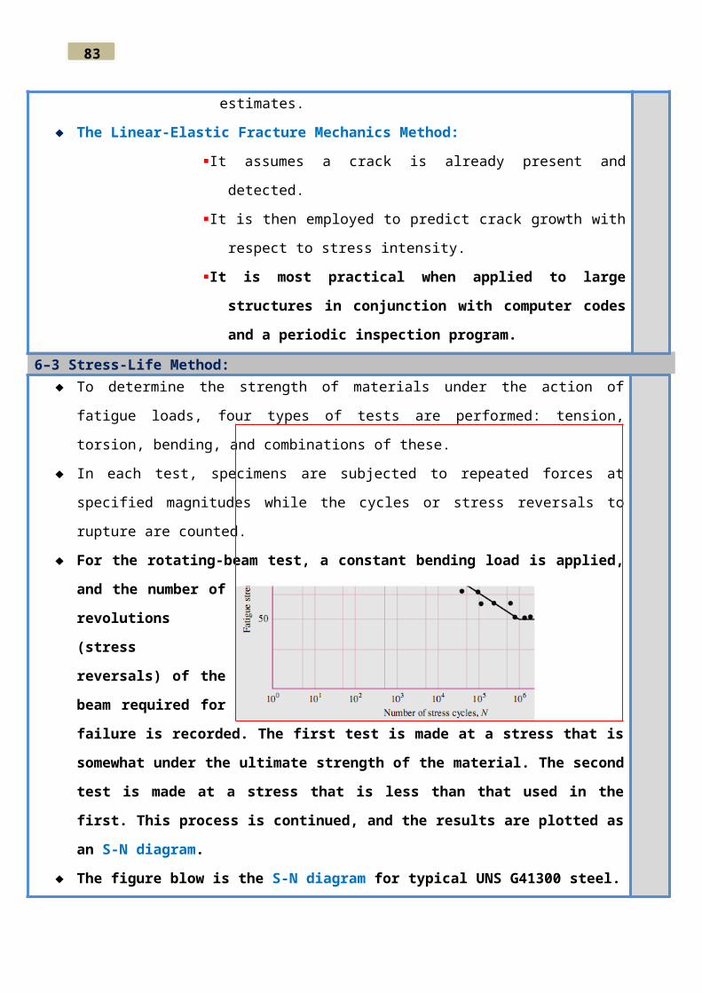
For the rotating-beam test, a constant bending load is applied, and the number of

revolutions (stress reversals) of the beam required for failure is recorded. The first test is

made at a stress that is somewhat under the ultimate strength of the material. The second

test is made at a stress that is less than that used in the first. This process is continued, and

the results are plotted as

an S-N diagram.

The figure blow is the S-

N diagram for typical

UNS G41300 steel.

It should be noted that

from the N-S diagram for

the case of steel:

A knee occurs around N=106 and beyond this knee failure will not occur, no

matter how great the number of cycles.

The strength corresponding to the knee is called the endurance limit Se , or the

83

fatigue limit.

For nonferrous metals and alloys, the graph of S-N diagram will never be

horizontal.

Meaning of N:

A stress cycle (N=1) constitutes a single application and removal of a load and then

another application and removal of the load in the opposite direction.

Thus, N=0.5, means the load is applied once and then removed, which is the case

with the simple tension test.

A body of knowledge available on fatigue failure from N=1 to N=103 cycles is

generally classified as low-cycle fatigue.

A stress cycles greater than ¿103 , is classified as high-cycle fatigue.

The boundary between the finite-life region and the infinite-life region can be

defined only for a specific material such as steel as shown above in which it lies

somewhere between N=106∧N=107

S-N method does not work well in low-cycle application, where the applied strains

have a significant plastic component.

Mischke has analyzed a great deal of actual teat data from several sources and concluded that

endurance limit can be related to tensile strength.

For Steel:

Se, ={ 0.5 Sut Sut ≤1460 MPa

700 MPaSut>1460 MPa

, where: Sut : : minimum tensile strength, and Se, : : rotating-beam specimen itself.

Aluminum and Magnesium alloys do not have an endurance limit, and the fatigue strength

is usually based on 5(108) cycles of stress reversal and it is given in table A-26 and A-27.

Endurance limits for various classes of cast irons, polished or machined, are given in table A-24

We could also use for Cast Iron and Cast Steel:

Se, ={ 0.45 Su t Su ≤600 MPa

275 MPaSut>600 MPa

The most widely used fatigue‐testing device is the R. R. Moore high–speed rotating-beam

machine. This machine subjects the specimen to pure bending (no transverse shear) by

means of weights. 

The specimen is very carefully machined and polished, with a final polishing in an

axial direction to avoid circumferential scratches. 

83

Other fatigue‐testing machines are available for applying fluctuating or reversed axial

stresses, torsional stresses, or combined stresses to the test reversed axial stresses, torsional

stresses, or combined stresses.

6–5 The Strain-Life Method:

The best approach yet advanced to explain the nature of fatigue failure is called by some the

strain-life method.

A fatigue failure almost always begins at a local discontinuity such as a notch, crack, or other

area of stress concentration.

When the stress at the discontinuity exceeds the elastic limit, plastic strain occurs.

If a fatigue fracture is to occur, there must exist cyclic plastic strains.

Thus we shall need to investigate the behavior of

materials subject to cyclic deformation.

Figure 6–2 has been constructed to show the general

appearance of these plots for the first few cycles of

controlled cyclic strain.

In this case the strength decreases with stress

repetitions, as evidenced by the fact that the

reversals occur at ever-smaller stress levels. As

previously noted, other materials may be

strengthened, instead, by cyclic stress reversals.

The graph has been reproduced as Fig. 6–2, to

explain the graph, we first define the following

terms:

Fatigue ductility coefficient ε F' is the true strain corresponding to fracture in one

reversal (point A in Fig. 6–3). The plastic-strain line begins at this point in Fig. 6–2.

Fatigue strength coefficient σ F' is the true stress corresponding to fracture in one

reversal (point A in Fig. 6–3). Note in Fig. 6–2 that the elastic-strain line begins at

σ F,

E.

Fatigue ductility exponent c is the slope of the plastic-strain line in Fig. 6–2 and is

the power to which the life 2N must be raised to be proportional to the true plastic-

strain amplitude. If the number of stress reversals is 2N, then N is the number of

cycles.

83

Fatigue strength exponent b is the slope of the elastic-strain line, and is the power to

which the life 2N must be raised to be proportional to the true-stress amplitude.

Now, from Fig. 6–3, we see that the total strain is the sum of the elastic and plastic

components. Therefore the total strain amplitude is half the total strain range:

∆ ε2

=∆ εe

2+

∆ ε p

2(a )

The equation of the plastic-strain line in Fig. 6–2 is:

∆ ε p

2=(ε F

, ) (2 N )c (6−1 )

The equation of the elastic strain line is:

∆ ε e

2=

σ F,

E(2 N )b (6−2 )

Therefore, from Eq. (a), we have for the total-strain amplitude:

∆ ε2

=(ε F, ) (2 N )c+

σF,

E(2 N )b (6−3 )

, which is the Manson-Coffin relationship between fatigue life and total strain.

6–6 The Linear-Elastic Fracture Mechanics Method: See Textbook Section 6-6 (p270-274).

A fatigue failure has an appearance similar to a brittle fracture, as the fracture surfaces are flat

and perpendicular to the stress axis with the absence of necking.

The fracture features of a fatigue failure, however, are quite different from a static brittle

fracture arising from three stages of development:

Stage I: Is the initiation of one or more micro-cracks due to cyclic plastic deformation followed

by crystallographic propagation extending from two to five grains about the origin.

Stage II: Progresses from micro-cracks to macro-cracks forming parallel-like fracture surfaces

separated by longitudinal ridges. The plateaus are generally smooth and normal to the direction

of maximum tensile stress. These surfaces can be wavy dark and light bands referred to as beach

marks or clamshell marks.

Stage III: Occurs during the final stress cycle when the remaining material cannot support the

loads, resulting in a sudden, fast fracture cannot support the loads, resulting in a sudden, fast

fracture.

6–7 The Endurance Limit:

83

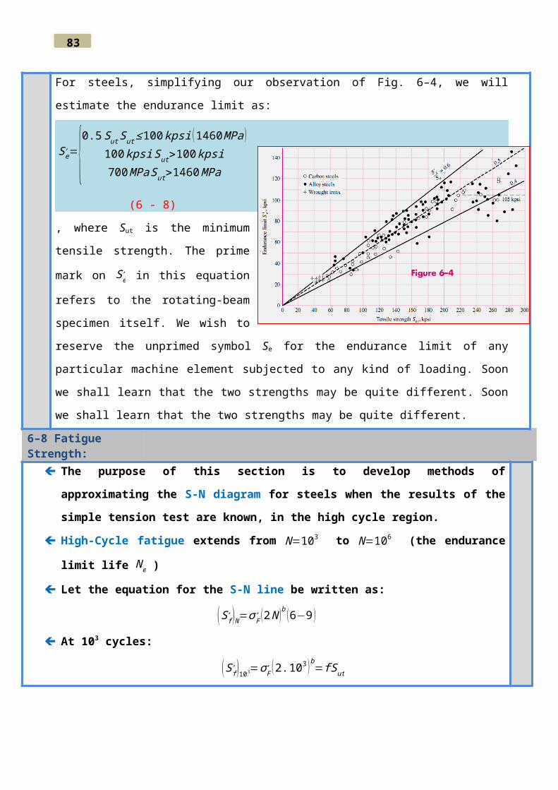
For steels, simplifying our observation of Fig. 6–4, we will estimate the endurance limit as:

Se, ={0.5 Sut Sut ≤100 kpsi (1460 MPa )

100 kpsi Sut>100 kpsi700 MPaSut>1460 MPa

(6 - 8)

, where Sut is the minimum tensile strength.

The prime mark on Se, in this equation

refers to the rotating-beam specimen itself.

We wish to reserve the unprimed symbol

Se for the endurance limit of any particular

machine element subjected to any kind of

loading. Soon we shall learn that the two

strengths may be quite different. Soon we

shall learn that the two strengths may be

quite different.

6–8 Fatigue Strength: The purpose of this section is to develop methods of approximating the S-N diagram for

steels when the results of the simple tension test are known, in the high cycle region.

High-Cycle fatigue extends from N=103 to N=106 (the endurance limit life N e )

Let the equation for the S-N line be written as:

(S f, )N=σ F

, (2 N )b (6−9 )

At 103 cycles:

(S f, )103=σ F

, (2.103 )b=fSut

83

, where f is the fraction of Sut represented by

(S f, )103

cycles . Solving for f gives:

83

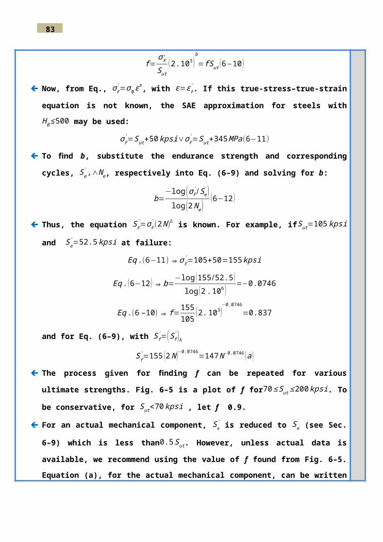
f =σ F

,

Sut

(2.103 )b

=fSut (6−10 )

Now, from Eq., σ F' =σ0 ε m, with ε=ε F

' . If this true-stress–true-strain equation is not known,

the SAE approximation for steels with HB ≤ 500 may be used:

σ F' =Sut+50 kpsi∨σ F

' =Sut+345 MPa(6−11)

To find b, substitute the endurance strength and corresponding cycles, Se' ,∧N e, respectively

into Eq. (6–9) and solving for b:

b=−log (σ F

' /Se' )

log (2 N e)(6−12 )

Thus, the equation SF' =σF

' (2 N )b is known. For example, ifSut=105 kpsiand Se' =52.5 kpsi at

failure:

Eq .(6−11)⇒ σ F' =105+50=155 kpsi

Eq . (6−12 )⇒b=−log (155/52.5 )

log (2 .106 )=−0.0746

Eq .(6 – 10)⇒ f =155105

(2.103 )−0.0746

=0.837

and for Eq. (6–9), with S f' =(S f

' )N

S f' =155 (2 N )−0.0746=147 N−0.0746 (a )

The process given for finding f can be repeated for various ultimate strengths. Fig. 6–5 is a

plot of f for70 ≤ Sut≤ 200 kpsi. To be conservative, for Sut<70 kpsi , let f 0.9.

For an actual mechanical component, Se' is reduced to Se (see Sec. 6–9) which is less than

0.5 Sut. However, unless actual data is available, we recommend using the value of f found

from Fig. 6–5. Equation (a), for the actual mechanical component, can be written in the

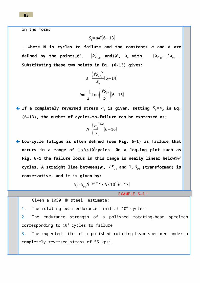
form:

S f=aN b (6−13 )

, where N is cycles to failure and the constants a and b are defined by the points103, ( S f )103

and106, Se with ( S f )103=f Sut . Substituting these two points in Eq. (6–13) gives:

a=(fSut )

2

Se

(6−14 )

b=−13

log( fSut

Se) (6−15 )

If a completely reversed stress σ a is given, setting S f=σ a in Eq. (6–13), the number of cycles-

83

to-failure can be expressed as:

N=( σa

a )1/b

(6−16 )

Low-cycle fatigue is often defined (see Fig. 6–1) as failure that occurs in a range of 1 ≤ N ≤ 103

cycles. On a log-log plot such as Fig. 6–1 the failure locus in this range is nearly linear below

103 cycles. A straight line between103, f Su t and 1 , Sut (transformed) is conservative, and it is

given by:

S f ≥ Sut N ( log f ) /3 1≤ N ≤103 (6−17 )

EXAMPLE 6–1:Given a 1050 HR steel, estimate:

1.The rotating-beam endurance limit at 106 cycles.

2.The endurance strength of a polished rotating-beam specimen corresponding to 104 cycles to failure

3.The expected life of a polished rotating-beam specimen under a completely reversed stress of 55

kpsi.

EXAMPLE 6-2:

83

6–9 Endurance Limit Modifying Factors:It is unrealistic to expect the endurance limit of a mechanical or structural member to match the

values obtained in the laboratory. Some differences include:

1. Material: composition, basis of failure, variability.

2. Manufacturing: method, heat treatment, fretting corrosion, surface condition,

stress concentration.

3. Environment: corrosion, temperature, stress state, relaxation times.

4. Design: size, shape, life, stress state, stress concentration, speed, fretting, galling.

Marin identified factors that quantified the effects of surface condition, size, loading,

temperature, and miscellaneous items. The Marin equation is therefore written as:

Se=ka kb kc kd k e k f Se' (6−18 )

, where:

k a=¿ surface condition modification factor

k b=¿ size modification factor

k c=¿load modification factor

k d=¿ temperature modification factor

k e=¿reliability factor

k f=¿miscellaneous-effects modification factor

83

Se' =¿rotary-beam test specimen endurance limit

Se=¿ endurance limit at the critical location of a machine part in the geometry and condition

of use

To account for the most important of these conditions, we employ a variety of modifying factors,

each of which is intended to account for a single effect. Or when endurance tests of parts are not

available, estimations are made by applying Marin factors to the endurance limit.

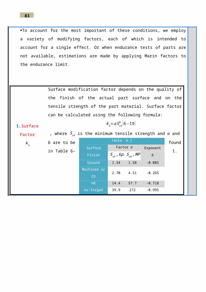
1.Surface Factor

k a

Surface modification factor depends on the quality of the finish of the actual

part surface and on the tensile strength of the part material. Surface factor can

be calculated using the following formula:

k a=a Sutb (6−19 )

, where Sut is the minimum tensile strength and a and b are to be found in Table

6–1.

2.Size Factor k b

i.Round bar in bending and in rotating: For bending and torsional loadings

there is a size effect, so:

k b={0.879 d−0.107 0.11≤ d ≤ 2∈¿0.91d−0.1572<d ≤ 10∈¿1.24 d−0.107 2.79≤ d ≤51 mm1.51 d−0.15751<d ≤ 254 mm

(6-20)

For axial loading there is no size effect, so:

k b=1 (6−21 )

ii. Round bar in bending is not rotating : The approach to be used here

employs an effective dimensionde, obtained by equating the volume of

material stressed at and above 95% of the maximum stress to the same

volume in the rotating-beam specimen.

A0.95σ=π4

[d2−0.95 d2 ]=0.0766 d2 (6−22 )

For non-rotating solid or hollow rounds, the 95 percent stress area is twice

Table 6.1

Surface FinishFactor a

Exponent bSut , kpsi Sut , MPa

Ground 1.34 1.58 -0.085

Machined or CD 2.70 4.51 -0.265

HR 14.4 57.7 -0.718

As-forged 39.9 272 -0.995

83

the area outside of two parallel chords having a spacing of 0.95d, where d is

the diameter. Using an exact computation, this is

A0.95σ=0.01046 d2 (6−23 )

, with de in Eq. (6–22), setting Eqs. (6–22) and (6–23) equal to each other

enables us to solve for the effective diameter. This gives:

de=0.370 d (6−24 )

iii. Noncircular cross section is used: A rectangular section of dimensions

h × b hasA0.95 σ=0.05 hb . Using the same approach as before:

de=0.808 (hb )12 (6−25 )

Table 6–2 provides A0.95σareas of common structural shapes undergoing

non-rotating bending.

3.Loading Factor,

kc

k c=¿(6-26)

For axial load we could also use the following formula:

k c={ 1 Sut>1520 MPa0.923 Sut>1520 MPa

4.Temperature

83

Factor kd

k d=0.975+0.432 ( 10−3 ) T F−0.115 (10−5 )T F2 +0.104 (10−8 ) T F

3 −0.595 (10−12 ) T F4 (6−27 )

Two types of problems arise when temperature is a consideration:

i. If the rotating- beam endurance limit is known at room temperature,

then use:

k d=ST

S RT

(6−28 )

from Table 6–3 or Eq. (6–27) and proceed as usual.

ii. If the rotating-beam endurance limit is not given, then compute it using

Eq. (6–8) and the temperature-corrected tensile strength obtained by

using the factor from Table 6–4. Then use k d=1.

5.Reliability

Factor ke

k e=1−0.08 za (6−29 )

83

, where za is defined by Eq. (20–16) and values for any desired reliability can be

determined from Table A–10. Table 6–4 gives reliability factors for some

standard specified reliability.

6.Miscellaneous-

Effects Factor kf

Read your textbook p.288

7.Stress

Concentration and

Notch Sensitivity

The factor Kf is commonly called a fatigue stress-concentration factor, and

hence the subscript f. So it is convenient to think of Kf as a stress-concentration

factor reduced from Kt because of lessened sensitivity to notches. The resulting

factor is defined by the equation:

K f =maximumstress∈notched specimen

stress∈notch−free specimen(a )

Notch sensitivity q is defined by the equation:

q=K f −1

K t−1∨qshear=

K f −1

K t−1(6−30 )

The fatigue stress-concentration factor, Kf then:

83

K f =1+q ( K t−1 )∨K fs=1+qshear ( K ts−1 ) (6−31 )

For steels and

2024

aluminum

alloys, use

Fig. 6–20 to

find q for

bending and

axial loading.

For shear

loading, use

Fig. 6–21.

Figure 6–20

has as its

basis the

Neuber

equation,

which is

given by:

K f =1+K t−1

1+√a/r(6−32 )

, where √a, is defined as the Neuber constant and is a material constant.

Equating Eqs. (6–30) and (6–32) yields the notch sensitivity equation:

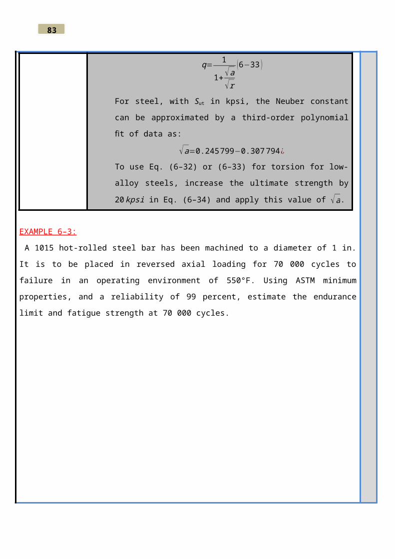
q= 1

1+ √a√r

(6−33 )

For steel, with Sut in kpsi, the Neuber constant can be approximated by a

third-order polynomial fit of data as:

√a=0.245 799−0.307 794 ¿

83

To use Eq. (6–32) or (6–33) for torsion for low-alloy steels, increase the

ultimate strength by 20 kpsi in Eq. (6–34) and apply this value of √a.

EXAMPLE 6–3:

A 1015 hot-rolled steel bar has been machined to a diameter of 1 in. It is to be placed in reversed axial

loading for 70 000 cycles to failure in an operating environment of 550°F. Using ASTM minimum

properties, and a reliability of 99 percent, estimate the endurance limit and fatigue strength at 70 000

cycles.

83

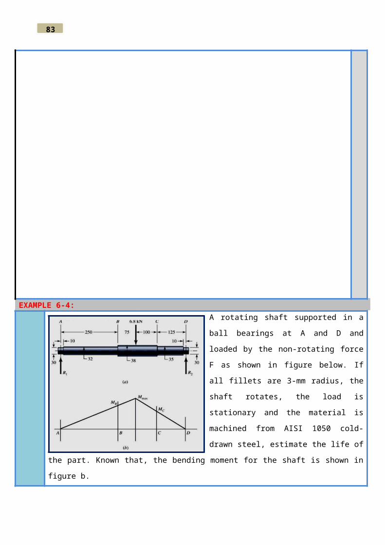
EXAMPLE 6-4:A rotating shaft supported in a ball bearings at A

and D and loaded by the non-rotating force F as

shown in figure below. If all fillets are 3-mm

radius, the shaft rotates, the load is stationary and

the material is machined from AISI 1050 cold-

drawn steel, estimate the life of the part. Known

that, the bending moment for the shaft is shown

in figure b.

83

6–11 Characterizing Fluctuating Stresses:Fluctuating stresses in machinery often

take the form of a sinusoidal pattern

because of the nature of some rotating

machinery.

It has been found that in periodic patterns

exhibiting a single maximum and a single

minimum of force, the shape of the wave

is not important, but the peaks on both the

high side (max.) and low side (min.) are

important.

In characterizing the force pattern. If

the largest force is Fmax and the smallest

force is Fmin , then a steady component

and an alternating component can be

constructed as follows:

Fm=Fmax+Fmin

2

Fa=Fmax−Fmin

2

, where Fm is the midrange steady component of force, and Fa is the amplitude of the alternating

component of force. Figure 6–7 illustrates some of the various stress-time traces that occur. The

following relationships and definitions are used when discussing mean and alternating stresses:,

some of which are shown in Fig. 6–7d, are:

σ min=minimum stress σm=midrangecomponent

σ max=maximumstress σ a=amplitude component

83

σ r=range of stress σ s=static∨steady stress

The following relations are evident from Fig. 6–7:

σ m=σmax+σmin

2σ a=|σmax−σ min

2 |(6−35 )

In addition to Eq. (6–35), the stress ratio, R:

R=σ min

σ max

(6−36 )

and the amplitude ratio, A:

A=σa

σm

(6−36 )

A steady or static stress is not the same as the mean stress. In fact, it may have any value

between min and max. The steady state exists because of a fixed load or preload applied to

the part, and it is usually independent of the varying portion of the load.

Notes:

For simple loading, it is acceptable to reduce the endurance limit by either dividing the un-

notched specimen endurance limit by Kf or multiplying the reversing stress by Kf (More safe

because it gives less life cycles).

For combined loading, which may involve more than one value of fatigue-concentration

factor, the stresses are multiplied by Kf.

In the case of absence of a notch, σ aand σ m are equal to the nominal stresses σ ao and σ mo

induced by loads Fa and Fm, respectively.

In the case of presence of a notch they are K f σao and K f σmo, respectively, as long as the

material remains without plastic strain. In other words, the fatigue stress concentration

factor K f is applied to both components.

When the steady stress component is high enough to induce localized notch yielding, the

designer has a problem. The material properties ( Sy and Sut) are new and difficult to

quantify. The nominal mean stress method (set σ a=K f σao∧σm=σmo) gives roughly

comparable results to the residual stress method, but both are approximations. For the

purposes of this course, for ductile materials in fatigue, the steady stress component stress-

concentration factor Kfm as:

83

K fm={ K f K f|σmax ,o|<S y

S y−K f σao

|σmo|K f|σ max, o|>S y

0 K f|σmax ,o−σmin ,o|>2 S y

(6−37 )

To avoid the localized plastic strain at a notch, set σ a=K f σao ,andσ m=K f σmo.

If the plastic strain at a notch cannot be avoided, then use Eqs. (6–37); or conservatively, set

σ a=K f σao, and useK f m=1 , that is, σ m=σ mo.

6–12 Fatigue Failure Criteria for Fluctuating Stress: Varying both the midrange stress and the

stress amplitude, or alternating component,

will give some information about the fatigue

resistance of parts when subjected to such

situations.

Three methods of plotting the results of such

tests are in general use and are shown in

figures 6.8, 6.9, and 6.10.

σ mPlotted along the x-axis.

All other components of stress plotted on the

y-axis.

The modified Goodman diagram (MGD)

consists of the lines constructed to Se (or

S f) above or below the origin.

Syis plotted on both axes, because Sy would be the criterion of failure if σ maxexceeded Sy.

Useful for analysis when all dimension of the part are known and the stress components can be

easily calculated. But it is difficult to use for design when the dimension are unknown.

The x-axis represents the ratio of the midrange strength Sm to the ultimate strength.

The y-axis represents the ratio of the alternating strength to the endurance limit.

83

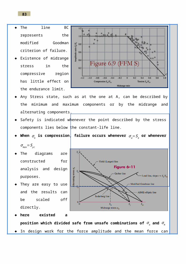
The line BC represents the

modified Goodman criterion of

failure.

Existence of midrange stress in

the compressive region has

little effect on the endurance

limit.

Any Stress state, such as at the

one at A, can be described by

the minimum and maximum

components or by the midrange and alternating components.

Safety is indicated whenever the point described by the stress components lies below the

constant-life line.

When σ m is compression,

failure occurs whenever

σ a=Se or whenever σ max=S yc

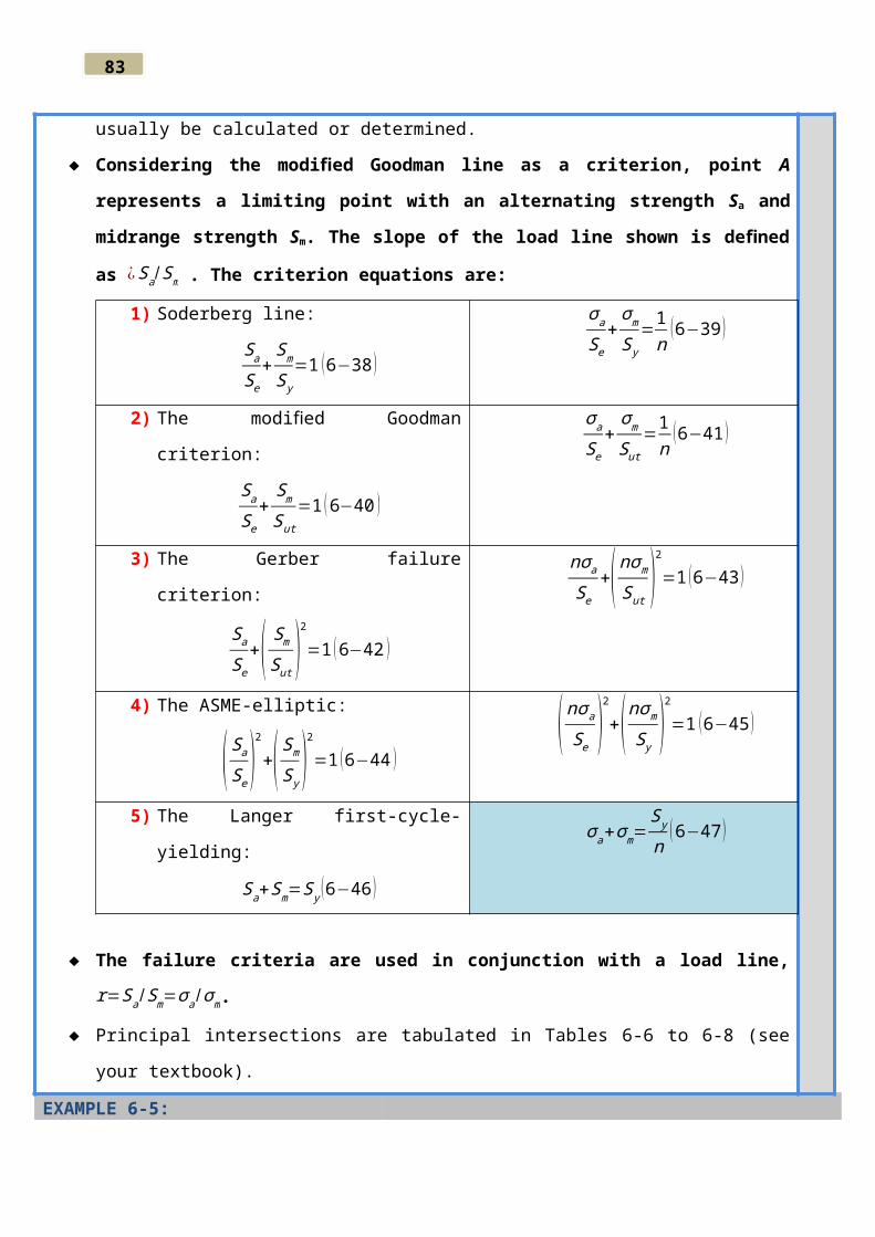
The diagrams are constructed

for analysis and design

purposes.

They are easy to use and the

results can be scaled off

directly.

here existed a position which

divided safe from unsafe combinations of σ a and σ m

In design work for the force amplitude and the mean force can usually be calculated or

determined.

Considering the modified Goodman line as a criterion, point A represents a limiting point

with an alternating strength Sa and midrange strength Sm. The slope of the load line shown

is defined as ¿ Sa/ Sm . The criterion equations are:

1) Soderberg line:

Sa

Se

+Sm

S y

=1 (6−38 )

σa

Se

+σm

S y

=1n

(6−39 )

83

2) The modified Goodman criterion:

Sa

Se

+Sm

Sut

=1 (6−40 )

σa

Se

+σm

Sut

=1n

(6−41 )

3) The Gerber failure criterion:

Sa

Se

+( Sm

Sut)

2

=1 (6−42 )

nσa

Se

+( nσm

Sut)

2

=1 (6−43 )

4) The ASME-elliptic:

( Sa

Se)

2

+( Sm

S y)

2

=1 (6−44 )( nσa

Se)

2

+( nσm

S y)

2

=1 (6−45 )

5) The Langer first-cycle-yielding:

Sa+Sm=S y (6−46 )σ a+σm=

S y

n(6−47 )

The failure criteria are used in conjunction with a load line, r=Sa/Sm=σa/σ m.

Principal intersections are tabulated in Tables 6-6 to 6-8 (see your textbook).

EXAMPLE 6-5:

83

Torsional Fatigue Strength under Fluctuating Stresses:The existence of a torsional steady-stress component not more than the torsional yield strength

has no effect on the torsional endurance limit, provide the material is ductile, polished, notch-

free, and cylindrical.

The torsional fatigue limit decreases monotonically with torsional steady stress when the material

83

has stress concentration, notches or surface imperfections.

In constructing the Goodman diagram:Ssu=0.67 Sut

Also, from chapter 5, Ssy=0.577 S yt from distortion-energy theory, and the mean load

factor kc is given by equation 6-26 or 0.577 for torsion.

Combinations of Loading Modes:

How do we proceed when the loading is a mixture of axial, bending, and torsional loads?

This type of loading introduces a few complications in that there may now exist combined

normal and shear stresses, each with alternating and midrange values, and several of the

factors used in determining the endurance limit depend on the type of loading. There may

also be multiple stress-concentration factors, one for each mode of loading. The problem of

how to deal with combined stresses was encountered when developing static failure theories.

The distortion energy failure theory proved to be a satisfactory method of combining the

multiple stresses on a stress element into a single equivalent von Mises stress. The same

approach will be used here:

1) The first step is to generate two stress elements—one for the alternating stresses and one for the

midrange stresses.

2) Next, apply the appropriate fatigue stress concentration factors to each of the stresses; i.e.,

apply ( K f )bending for the bending stresses, ( K fs)torsionfor the torsional stresses, and ( K f )axialfor the

axial stresses. Then calculate an equivalent von Mises stress for each of these two stress

elements,σ a' , and σ m

' . For the endurance limit,Se, use the endurance limit modifiers,

k a , k b ,¿k c for bending stress only and do not use k cnor divide by K f or K f s . If axial stress is

present divide the alternating axial stress only by k c=0.85 . For the special case of

combined bending, torsional shear, and axial stresses:

σ a' ={[ ( K f )bending (σ a )bending+( K f )axizl

(σ a )axial

o .85 ]2

+3 [ ( K fs) torsion( τa )torsion ]2}12

(6−48 )

σ m' ={[ ( K f )bending (σ m )bending+( K f )axizl ( σm )axial ]

2+3 [ ( K fs)torsion ( τm )torsion ]2}

12 (6−49 )

3) Finally, select a fatigue failure criterion {modified Goodman, Gerber, ASME-elliptic, or

Soderberg [see Eq. (6–38) to (6–47)]} to complete the fatigue analysis.

4) Conservative check for localized yielding using von Mises stresses, as:

σ a' +σm

' =S y

n(6−50 )

5) For first-cycle localized yielding, the maximum von Mises stress is calculated. Then

83

substitute σmax and τmax into the equation for the von Mises stress. A simpler and more

conservative method is to add Eq. (6–48) and Eq. (6–49). That is, σ max' =σa

' +σ m' .

Example 6-6:A 38 mm diameter bar has been machined from AISI 1050 CD steel. This part is to withstand a

fluctuating tensile load varying from zero to 71.2kN. Because of the ends and the fillet radius, a

fatigue stress-concentration factor K f is 1.85 for 106 or larger life. Find Sa , Sm, and the factor of

safety guarding against fatigue (n f) and first-cycle yielding (n y) using (a) Gerber method and (b)

Goodman method.

6–15 Varying, Fluctuating Stresses; Cumulative Fatigue Damage:The method used here amounts to a variation of the rain-flow counting technique. The Palmgren-Miner

cycle-ratio summation rule, also called Miner’s rule, is written as:

C=∑ ni

N i

(6−51 )

, where ni is the number of cycles at stress level σi and Ni is the number of cycles to failure at stress

level σi. The parameter C has been determined by experiment; it is usually found in the range

0.7<c<2.2 with an average value near unity.

Using the deterministic formulation as a linear damage rule we write:

83

D=∑ ni

N i

(6−52 )

, where D is the accumulated damage. When D = c = 1 , failure ensues. And the total number of cycles

is obtained as:

D=∑ ∝i

N i

≥1N

∧∝i=ni

N(6−53 )

Problem6–30

A machine part will be cycled at ± 48 kpsi for 4 (103) cycles. Then the loading will be changed to

± 38 kpsi for 6 (104) cycles. Finally, the load will be changed to ± 32 kpsi. How many cycles of operation

can be expected at this stress level? For the part, Sut=76 kpsi, f =0.9 , and has a fully corrected endurance

strength of Se=30 kpsi. (a) Use Miner’s method. (b) Use Manson’s method.

83

Problem6–31

A rotating-beam specimen with an endurance limit of 50 kpsi and an ultimate strength of 100 kpsi

is cycled 20 percent of the time at 70 kpsi, 50 percent at 55 kpsi, and 30 percent at 40 kpsi. Let

f =0.9 and estimate the number of cycles to failure.

Problem6–8

A solid round bar, 25 mm in diameter, has a groove 2.5-mm deep with a 2.5-mm radius

machined into it. The bar is made of AISI 1018 CD steel and is subjected to a purely

reversing torque of 200 N · m. For the S-N curve of this material, let f = 0.9 . (a) Estimate

the number of cycles to failure. (b) If the bar is also placed in an environment with a

temperature of 450 oC , estimate the number of cycles to failure.

83

Problem6–17

The cold-drawn AISI 1018 steel bar shown in the figure is subjected to an axial load

fluctuating between 800 and 3000 lbf. Estimate the factors of safety ny and nf using (a) a

Gerber fatigue failure criterion as part of the designer’s fatigue diagram, and (b) an ASME-

elliptic fatigue failure criterion as part of the designer’s fatigue diagram.

83