Embed Size (px)
Citation preview
Structural Analysis IV Chapter 5 – Structural Dynamics
Dr. C. Caprani 1
Chapter 5 - Structural Dynamics
5.1 Introduction ......................................................................................................... 3
5.1.1 Outline of Structural Dynamics ..................................................................... 3
5.1.2 An Initial Numerical Example ....................................................................... 5
5.1.3 Case Study – Aberfeldy Footbridge, Scotland .............................................. 8
5.1.4 Structural Damping ...................................................................................... 10
5.2 Single Degree-of-Freedom Systems ................................................................. 11
5.2.1 Fundamental Equation of Motion ................................................................ 11
5.2.2 Free Vibration of Undamped Structures...................................................... 16
5.2.3 Computer Implementation & Examples ...................................................... 20
5.2.4 Free Vibration of Damped Structures .......................................................... 26
5.2.5 Computer Implementation & Examples ...................................................... 30
5.2.6 Estimating Damping in Structures ............................................................... 33
5.2.7 Response of an SDOF System Subject to Harmonic Force ........................ 35
5.2.8 Computer Implementation & Examples ...................................................... 42
5.2.9 Numerical Integration – Newmark‟s Method ............................................. 47
5.2.10 Computer Implementation & Examples ................................................... 53
5.2.11 Problems ................................................................................................... 59
5.3 Multi-Degree-of-Freedom Systems .................................................................. 63
5.3.1 General Case (based on 2DOF) ................................................................... 63
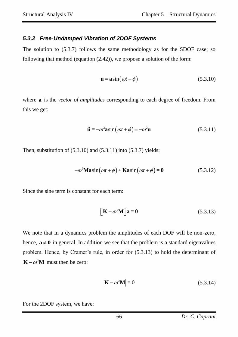
5.3.2 Free-Undamped Vibration of 2DOF Systems ............................................. 66
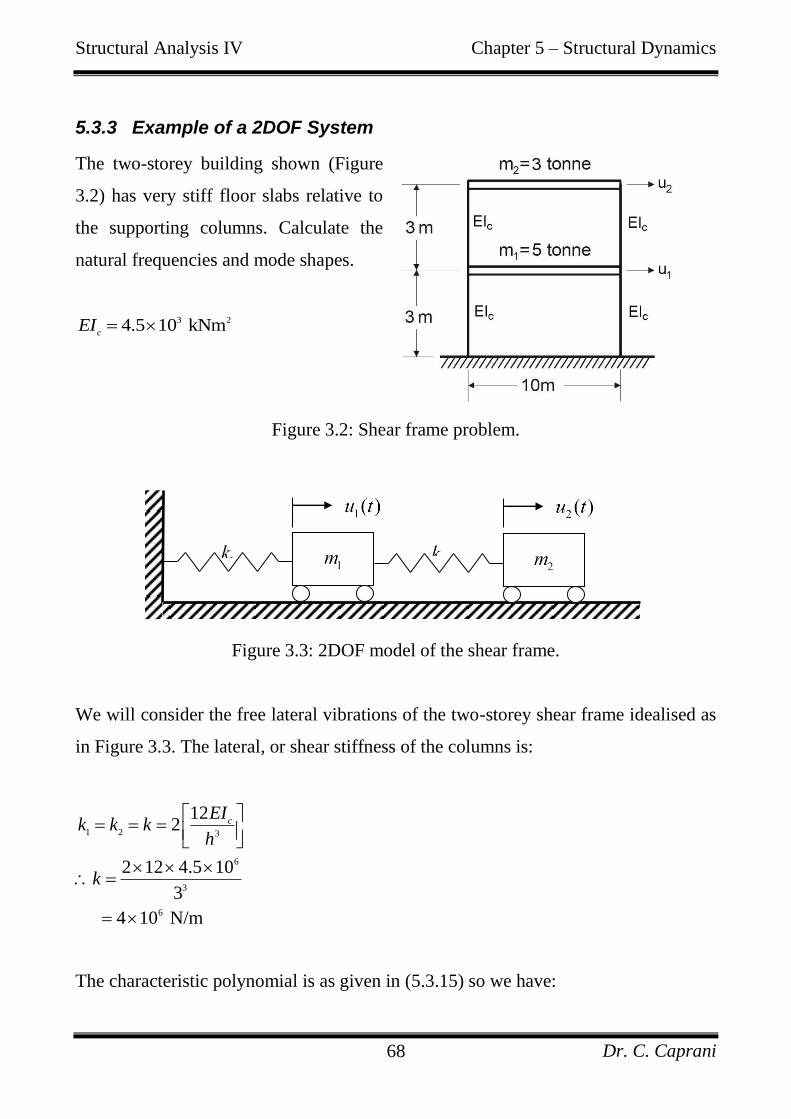
5.3.3 Example of a 2DOF System ........................................................................ 68
5.3.4 Case Study – Aberfeldy Footbridge, Scotland ............................................ 73
Structural Analysis IV Chapter 5 – Structural Dynamics
Dr. C. Caprani 2
5.4 Continuous Structures ...................................................................................... 76
5.4.1 Exact Analysis for Beams ............................................................................ 76
5.4.2 Approximate Analysis – Bolton‟s Method .................................................. 86
5.4.3 Problems ...................................................................................................... 95
5.5 Practical Design Considerations ...................................................................... 97
5.5.1 Human Response to Dynamic Excitation .................................................... 97
5.5.2 Crowd/Pedestrian Dynamic Loading .......................................................... 99
5.5.3 Damping in Structures ............................................................................... 107
5.5.4 Design Rules of Thumb ............................................................................. 109
5.6 Appendix .......................................................................................................... 114
5.6.1 Past Exam Questions ................................................................................. 114
5.6.2 References .................................................................................................. 121
5.6.3 Amplitude Solution to Equation of Motion ............................................... 123
5.6.4 Solutions to Differential Equations ........................................................... 125
5.6.5 Important Formulae ................................................................................... 134
5.6.6 Glossary ..................................................................................................... 139
Rev. 1
Structural Analysis IV Chapter 5 – Structural Dynamics
Dr. C. Caprani 3
5.1 Introduction
5.1.1 Outline of Structural Dynamics
Modern structures are increasingly slender and have reduced redundant strength due
to improved analysis and design methods. Such structures are increasingly responsive
to the manner in which loading is applied with respect to time and hence the dynamic
behaviour of such structures must be allowed for in design; as well as the usual static
considerations. In this context then, the word dynamic simply means “changes with
time”; be it force, deflection or any other form of load effect.
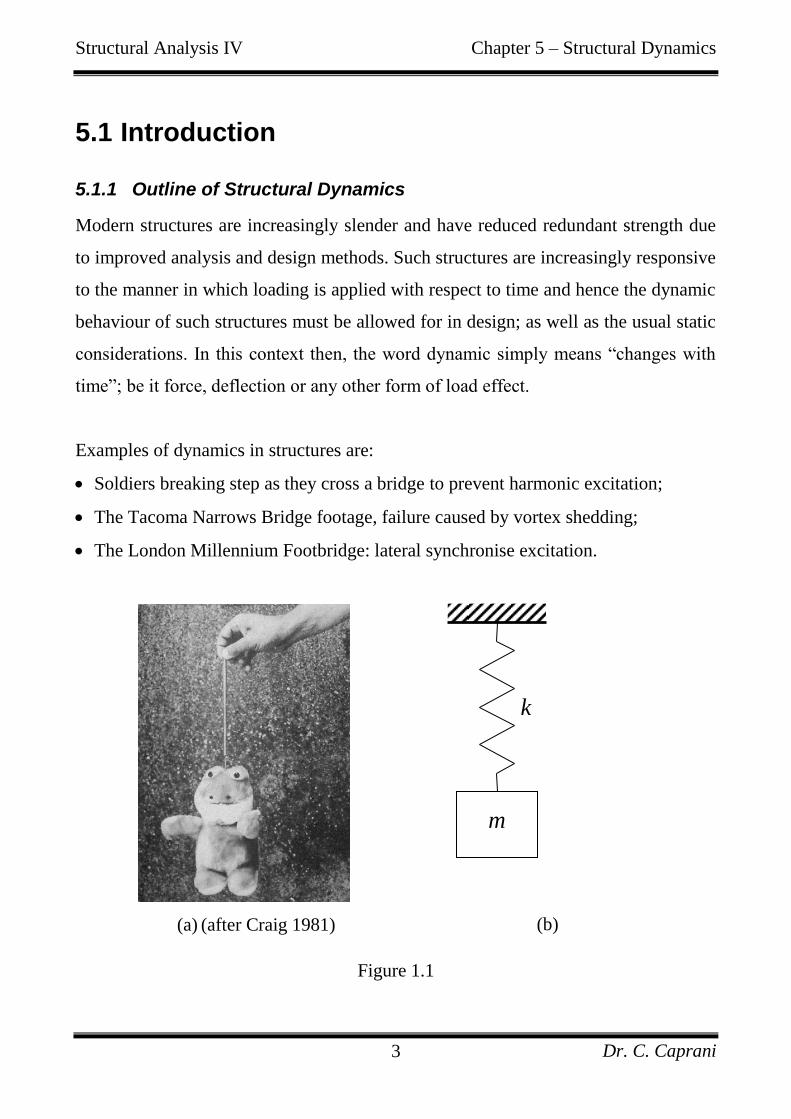
Examples of dynamics in structures are:
Soldiers breaking step as they cross a bridge to prevent harmonic excitation;
The Tacoma Narrows Bridge footage, failure caused by vortex shedding;
The London Millennium Footbridge: lateral synchronise excitation.
(a) (after Craig 1981)
(b)
Figure 1.1
m
k
Structural Analysis IV Chapter 5 – Structural Dynamics
Dr. C. Caprani 4
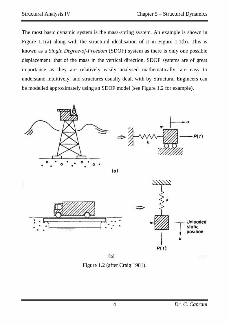
The most basic dynamic system is the mass-spring system. An example is shown in
Figure 1.1(a) along with the structural idealisation of it in Figure 1.1(b). This is
known as a Single Degree-of-Freedom (SDOF) system as there is only one possible
displacement: that of the mass in the vertical direction. SDOF systems are of great
importance as they are relatively easily analysed mathematically, are easy to
understand intuitively, and structures usually dealt with by Structural Engineers can
be modelled approximately using an SDOF model (see Figure 1.2 for example).
Figure 1.2 (after Craig 1981).
Structural Analysis IV Chapter 5 – Structural Dynamics
Dr. C. Caprani 5
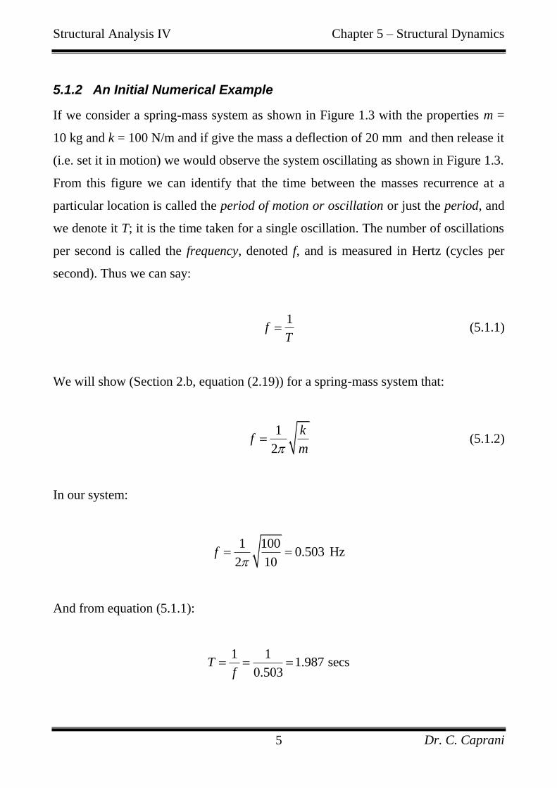
5.1.2 An Initial Numerical Example
If we consider a spring-mass system as shown in Figure 1.3 with the properties m =
10 kg and k = 100 N/m and if give the mass a deflection of 20 mm and then release it
(i.e. set it in motion) we would observe the system oscillating as shown in Figure 1.3.
From this figure we can identify that the time between the masses recurrence at a
particular location is called the period of motion or oscillation or just the period, and
we denote it T; it is the time taken for a single oscillation. The number of oscillations
per second is called the frequency, denoted f, and is measured in Hertz (cycles per
second). Thus we can say:
1
fT
(5.1.1)
We will show (Section 2.b, equation (2.19)) for a spring-mass system that:
1
2
kf
m (5.1.2)
In our system:
1 1000.503 Hz
2 10f
And from equation (5.1.1):
1 11.987 secs
0.503T
f
Structural Analysis IV Chapter 5 – Structural Dynamics
Dr. C. Caprani 6
We can see from Figure 1.3 that this is indeed the period observed.
Figure 1.3
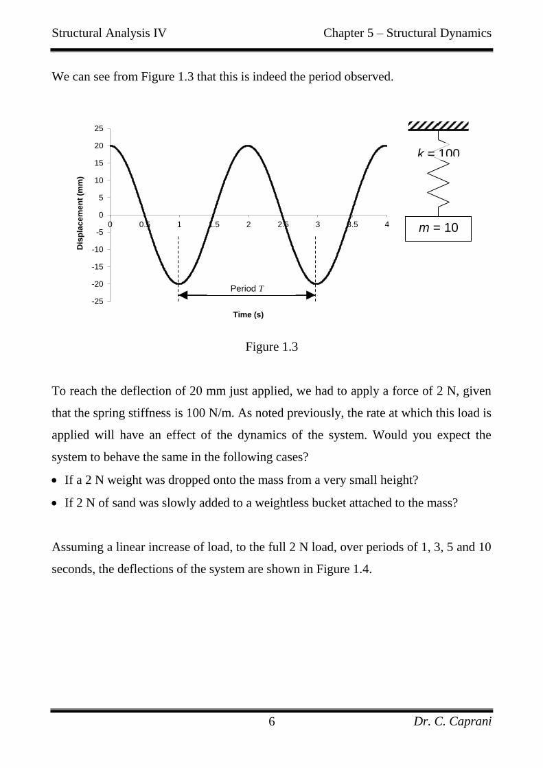
To reach the deflection of 20 mm just applied, we had to apply a force of 2 N, given
that the spring stiffness is 100 N/m. As noted previously, the rate at which this load is
applied will have an effect of the dynamics of the system. Would you expect the
system to behave the same in the following cases?
If a 2 N weight was dropped onto the mass from a very small height?
If 2 N of sand was slowly added to a weightless bucket attached to the mass?
Assuming a linear increase of load, to the full 2 N load, over periods of 1, 3, 5 and 10
seconds, the deflections of the system are shown in Figure 1.4.
-25
-20
-15
-10
-5
0
5
10
15
20
25
0 0.5 1 1.5 2 2.5 3 3.5 4
Dis
pla
ce
me
nt
(mm
)
Time (s)
Period T
m = 10
k = 100

Structural Analysis IV Chapter 5 – Structural Dynamics
Dr. C. Caprani 7
Figure 1.4
Remembering that the period of vibration of the system is about 2 seconds, we can
see that when the load is applied faster than the period of the system, large dynamic
effects occur. Stated another way, when the frequency of loading (1, 0.3, 0.2 and 0.1
Hz for our sample loading rates) is close to, or above the natural frequency of the
system (0.5 Hz in our case), we can see that the dynamic effects are large.
Conversely, when the frequency of loading is less than the natural frequency of the
system little dynamic effects are noticed – most clearly seen via the 10 second ramp-
up of the load, that is, a 0.1 Hz load.
0
5
10
15
20
25
30
35
40
0 2 4 6 8 10 12 14 16 18 20
Defl
ecti
on
(m
m)
Time (s)
Dynamic Effect of Load Application Duration
1-sec
3-sec
5-sec
10-sec
Structural Analysis IV Chapter 5 – Structural Dynamics
Dr. C. Caprani 8
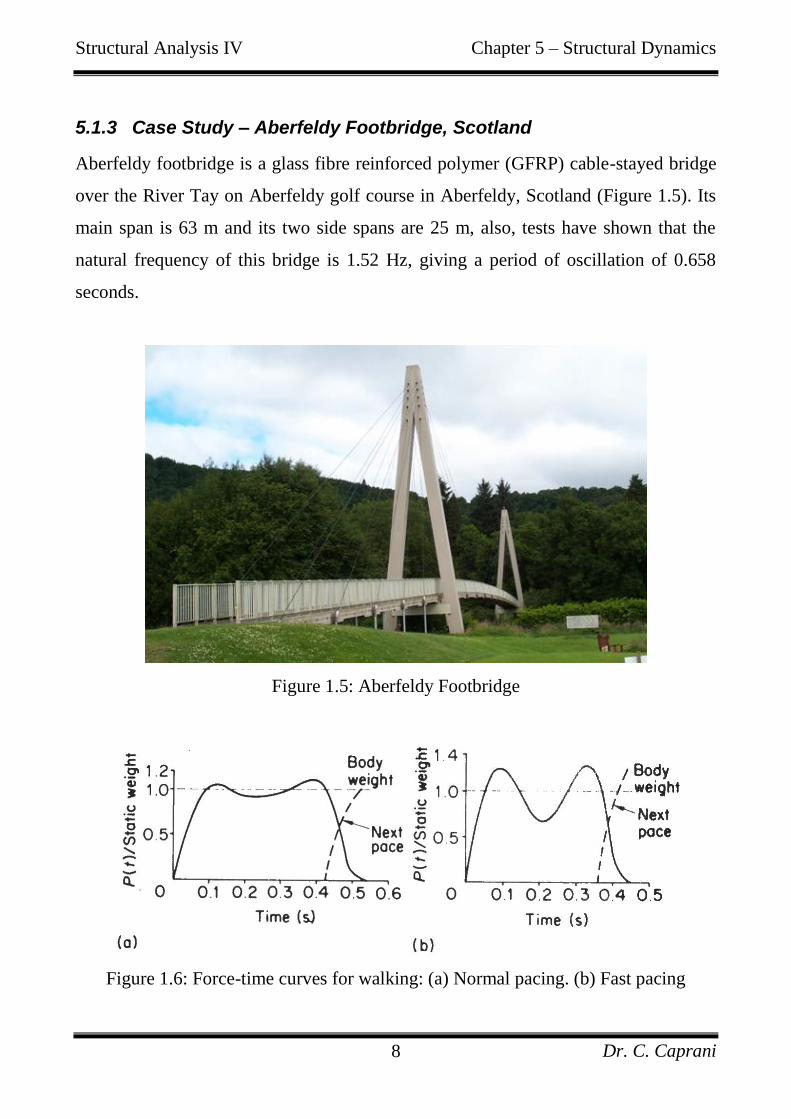
5.1.3 Case Study – Aberfeldy Footbridge, Scotland
Aberfeldy footbridge is a glass fibre reinforced polymer (GFRP) cable-stayed bridge
over the River Tay on Aberfeldy golf course in Aberfeldy, Scotland (Figure 1.5). Its
main span is 63 m and its two side spans are 25 m, also, tests have shown that the
natural frequency of this bridge is 1.52 Hz, giving a period of oscillation of 0.658
seconds.
Figure 1.5: Aberfeldy Footbridge
Figure 1.6: Force-time curves for walking: (a) Normal pacing. (b) Fast pacing
Structural Analysis IV Chapter 5 – Structural Dynamics
Dr. C. Caprani 9
Footbridges are generally quite light structures as the loading consists of pedestrians;
this often results in dynamically lively structures. Pedestrian loading varies as a
person walks; from about 0.65 to 1.3 times the weight of the person over a period of
about 0.35 seconds, that is, a loading frequency of about 2.86 Hz (Figure 1.6). When
we compare this to the natural frequency of Aberfeldy footbridge we can see that
pedestrian loading has a higher frequency than the natural frequency of the bridge –
thus, from our previous discussion we would expect significant dynamic effects to
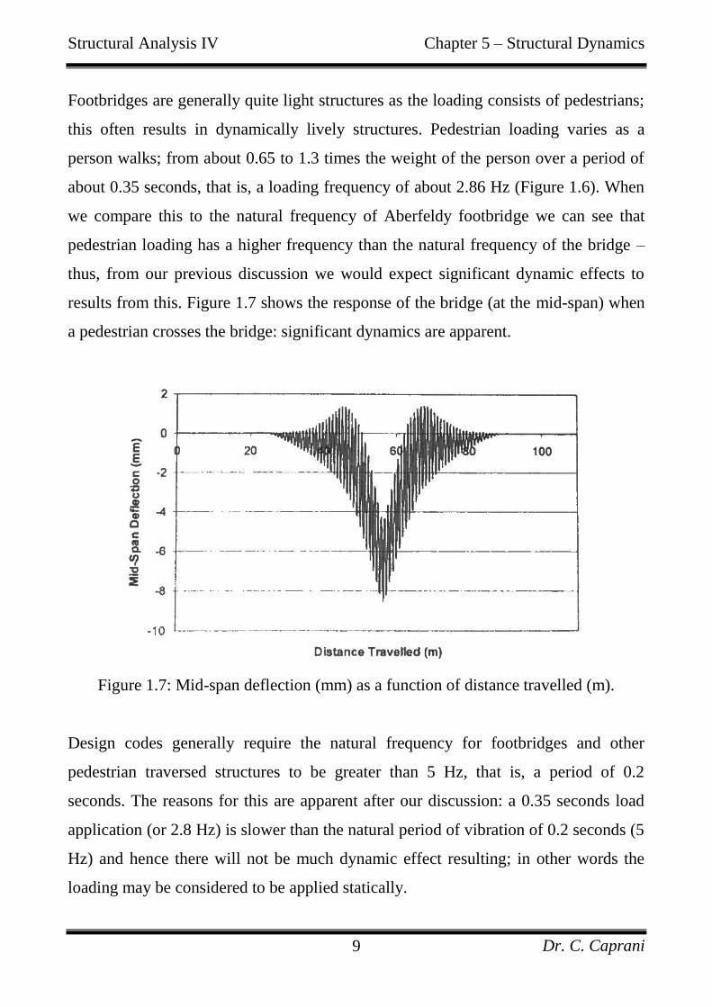
results from this. Figure 1.7 shows the response of the bridge (at the mid-span) when
a pedestrian crosses the bridge: significant dynamics are apparent.
Figure 1.7: Mid-span deflection (mm) as a function of distance travelled (m).
Design codes generally require the natural frequency for footbridges and other
pedestrian traversed structures to be greater than 5 Hz, that is, a period of 0.2
seconds. The reasons for this are apparent after our discussion: a 0.35 seconds load
application (or 2.8 Hz) is slower than the natural period of vibration of 0.2 seconds (5
Hz) and hence there will not be much dynamic effect resulting; in other words the
loading may be considered to be applied statically.
Structural Analysis IV Chapter 5 – Structural Dynamics
Dr. C. Caprani 10
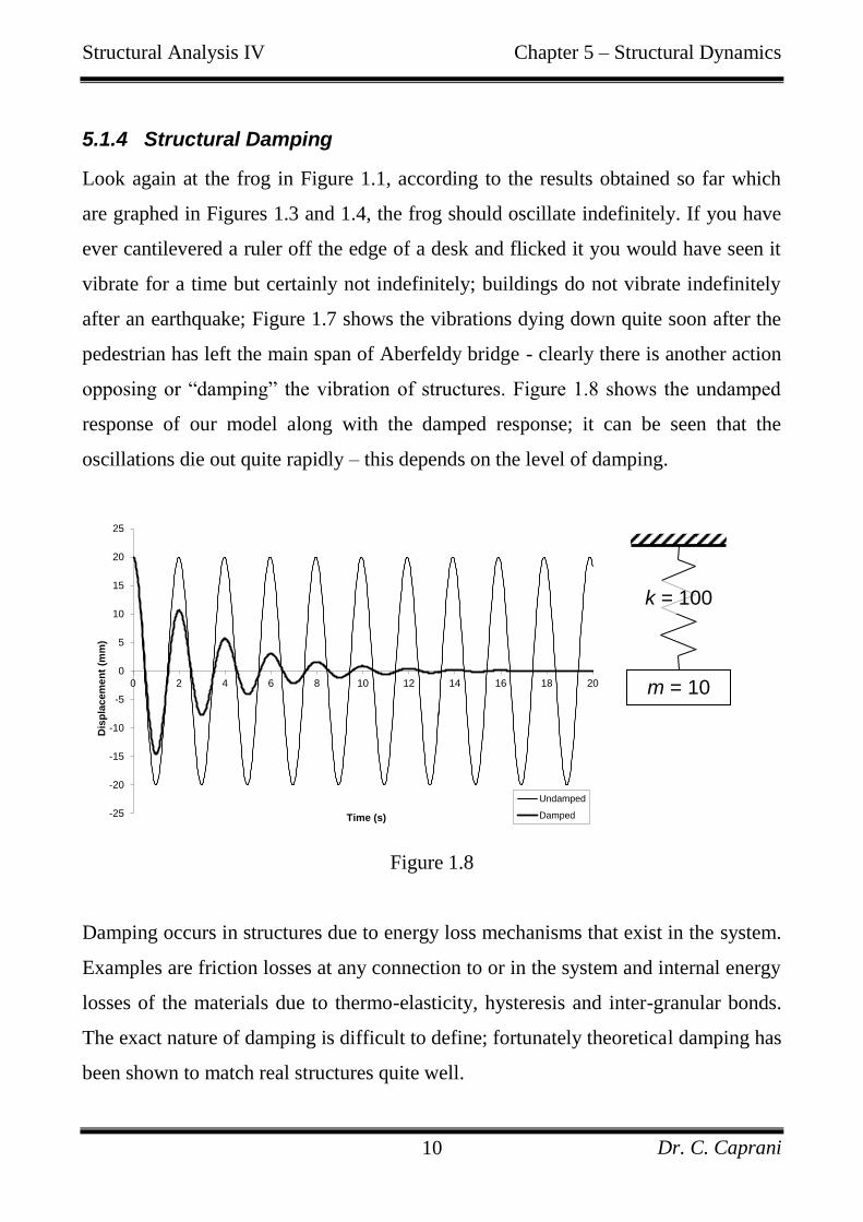
5.1.4 Structural Damping
Look again at the frog in Figure 1.1, according to the results obtained so far which
are graphed in Figures 1.3 and 1.4, the frog should oscillate indefinitely. If you have
ever cantilevered a ruler off the edge of a desk and flicked it you would have seen it
vibrate for a time but certainly not indefinitely; buildings do not vibrate indefinitely
after an earthquake; Figure 1.7 shows the vibrations dying down quite soon after the
pedestrian has left the main span of Aberfeldy bridge - clearly there is another action
opposing or “damping” the vibration of structures. Figure 1.8 shows the undamped
response of our model along with the damped response; it can be seen that the
oscillations die out quite rapidly – this depends on the level of damping.
Figure 1.8
Damping occurs in structures due to energy loss mechanisms that exist in the system.
Examples are friction losses at any connection to or in the system and internal energy
losses of the materials due to thermo-elasticity, hysteresis and inter-granular bonds.
The exact nature of damping is difficult to define; fortunately theoretical damping has
been shown to match real structures quite well.
-25
-20
-15
-10
-5
0
5
10
15
20
25
0 2 4 6 8 10 12 14 16 18 20
Dis
pla
cem
en
t (m
m)
Time (s)
Undamped
Damped
m = 10
k = 100
Structural Analysis IV Chapter 5 – Structural Dynamics
Dr. C. Caprani 11
5.2 Single Degree-of-Freedom Systems
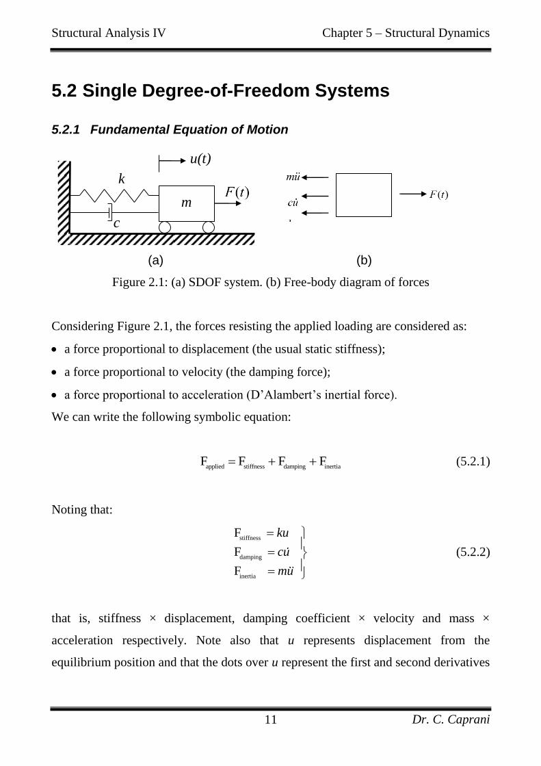
5.2.1 Fundamental Equation of Motion
(a) (b)
Figure 2.1: (a) SDOF system. (b) Free-body diagram of forces
Considering Figure 2.1, the forces resisting the applied loading are considered as:
a force proportional to displacement (the usual static stiffness);
a force proportional to velocity (the damping force);
a force proportional to acceleration (D‟Alambert‟s inertial force).
We can write the following symbolic equation:
applied stiffness damping inertia
F F F F (5.2.1)
Noting that:
stiffness
damping
inertia
F
F
F
ku
cu
mu
(5.2.2)
that is, stiffness × displacement, damping coefficient × velocity and mass ×
acceleration respectively. Note also that u represents displacement from the
equilibrium position and that the dots over u represent the first and second derivatives
m
k
u(t)
c
Structural Analysis IV Chapter 5 – Structural Dynamics
Dr. C. Caprani 12
with respect to time. Thus, noting that the displacement, velocity and acceleration are
all functions of time, we have the Fundamental Equation of Motion:
mu t cu t ku t F t (5.2.3)
In the case of free vibration, there is no forcing function and so 0F t which gives
equation (5.2.3) as:
0mu t cu t ku t (5.2.4)
We note also that the system will have a state of initial conditions:
00u u (5.2.5)
00u u (5.2.6)
In equation (5.2.4), dividing across by m gives:
( ) ( ) ( ) 0c k
u t u t u tm m
(5.2.7)
We introduce the following notation:
cr
c
c (5.2.8)
2 k
m (5.2.9)
Structural Analysis IV Chapter 5 – Structural Dynamics
Dr. C. Caprani 13
Or equally,
k
m (5.2.10)
In which
is called the undamped circular natural frequency and its units are radians per
second (rad/s);
is the damping ratio which is the ratio of the damping coefficient, c, to the
critical value of the damping coefficient cr
c .
We will see what these terms physically mean. Also, we will later see (equation
(5.2.18)) that:
2 2cr
c m km (5.2.11)
Equations (5.2.8) and (5.2.11) show us that:
2c
m (5.2.12)
When equations (5.2.9) and (5.2.12) are introduced into equation (5.2.7), we get the
prototype SDOF equation of motion:
22 0u t u t u t (5.2.13)
In considering free vibration only, the general solution to (5.2.13) is of a form
tu Ce (5.2.14)
Structural Analysis IV Chapter 5 – Structural Dynamics
Dr. C. Caprani 14
When we substitute (5.2.14) and its derivates into (5.2.13) we get:
2 22 0tCe (5.2.15)
For this to be valid for all values of t, tCe cannot be zero. Thus we get the
characteristic equation:
2 22 0 (5.2.16)
the solutions to this equation are the two roots:
2 2 2
1,2
2
2 4 4
2
1
(5.2.17)
Therefore the solution depends on the magnitude of relative to 1. We have:
1 : Sub-critical damping or under-damped;
Oscillatory response only occurs when this is the case – as it is for almost all
structures.
1 : Critical damping;
No oscillatory response occurs.
1 : Super-critical damping or over-damped;
No oscillatory response occurs.
Therefore, when 1 , the coefficient of ( )u t in equation (5.2.13) is, by definition,
the critical damping coefficient. Thus, from equation (5.2.12):
Structural Analysis IV Chapter 5 – Structural Dynamics
Dr. C. Caprani 15
2 crc
m (5.2.18)
From which we get equation (5.2.11).
Structural Analysis IV Chapter 5 – Structural Dynamics
Dr. C. Caprani 16
5.2.2 Free Vibration of Undamped Structures
We will examine the case when there is no damping on the SDOF system of Figure
2.1 so 0 in equations (5.2.13), (5.2.16) and (5.2.17) which then become:
2 0u t u t (5.2.19)
respectively, where 1i . From the Appendix we see that the general solution to
this equation is:
cos sinu t A t B t (5.2.20)
where A and B are constants to be obtained from the initial conditions of the system,
equations (5.2.5) and (5.2.6). Thus, at 0t , from equation (5.2.20):
00 cos 0 sin 0u A B u
0
A u (5.2.21)
From equation (5.2.20):
sin cosu t A t B t (5.2.22)
And so:
0
0
0 sin 0 cos 0u A B u
B u
0u
B
(5.2.23)
Structural Analysis IV Chapter 5 – Structural Dynamics
Dr. C. Caprani 17
Thus equation (5.2.20), after the introduction of equations (5.2.21) and (5.2.23),
becomes:
0
0cos sin
uu t u t t
(5.2.24)
where 0
u and 0
u are the initial displacement and velocity of the system respectively.
Noting that cosine and sine are functions that repeat with period 2 , we see that
1 12t T t (Figure 2.3) and so the undamped natural period of the SDOF
system is:
2
T
(5.2.25)
The natural frequency of the system is got from (1.1), (5.2.25) and (5.2.9):
1 1
2 2
kf
T m
(5.2.26)
and so we have proved (1.2). The importance of this equation is that it shows the
natural frequency of structures to be proportional to km
. This knowledge can aid a
designer in addressing problems with resonance in structures: by changing the
stiffness or mass of the structure, problems with dynamic behaviour can be
addressed.
Structural Analysis IV Chapter 5 – Structural Dynamics
Dr. C. Caprani 18
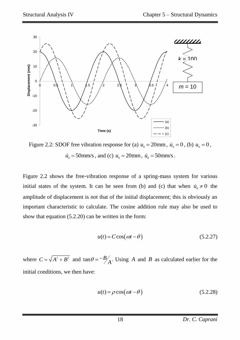
Figure 2.2: SDOF free vibration response for (a) 0
20mmu , 0
0u , (b) 0
0u ,
050mm/su , and (c)
020mmu ,
050mm/su .
Figure 2.2 shows the free-vibration response of a spring-mass system for various
initial states of the system. It can be seen from (b) and (c) that when 0
0u the
amplitude of displacement is not that of the initial displacement; this is obviously an
important characteristic to calculate. The cosine addition rule may also be used to
show that equation (5.2.20) can be written in the form:
( ) cosu t C t (5.2.27)
where 2 2C A B and tan BA
. Using A and B as calculated earlier for the
initial conditions, we then have:
( ) cosu t t (5.2.28)
-30
-20
-10
0
10
20
30
0 0.5 1 1.5 2 2.5 3 3.5 4
Dis
pla
cem
en
t (m
m)
Time (s)
(a)
(b)
(c)
m = 10
k = 100
Structural Analysis IV Chapter 5 – Structural Dynamics
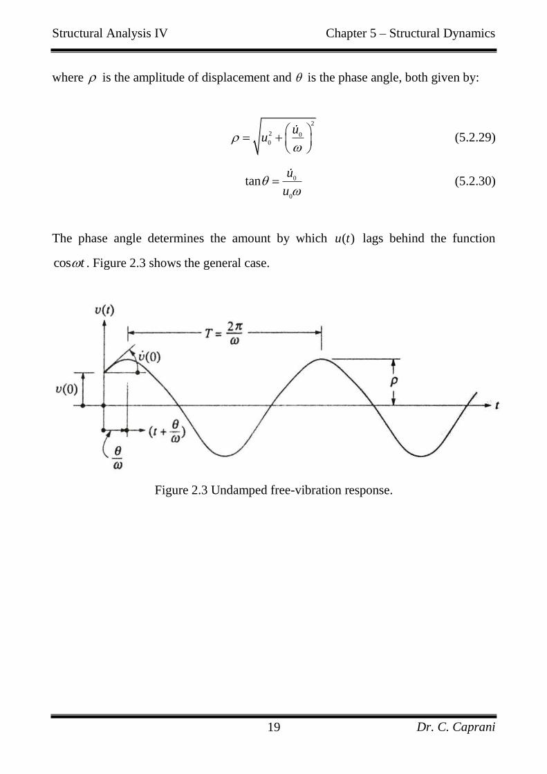
Dr. C. Caprani 19
where is the amplitude of displacement and is the phase angle, both given by:
2
2 0
0
uu
(5.2.29)
0
0
tanu
u
(5.2.30)
The phase angle determines the amount by which ( )u t lags behind the function
cos t . Figure 2.3 shows the general case.
Figure 2.3 Undamped free-vibration response.
Structural Analysis IV Chapter 5 – Structural Dynamics
Dr. C. Caprani 20
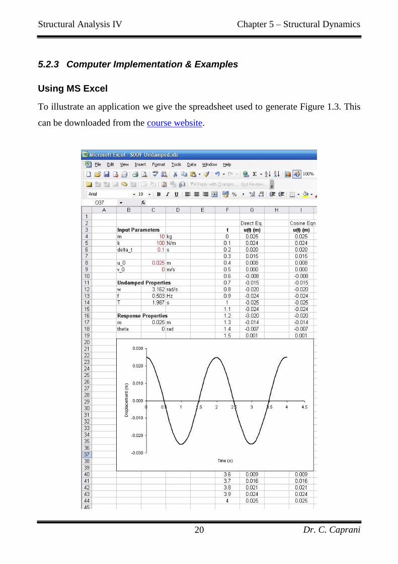
5.2.3 Computer Implementation & Examples
Using MS Excel
To illustrate an application we give the spreadsheet used to generate Figure 1.3. This
can be downloaded from the course website.
Structural Analysis IV Chapter 5 – Structural Dynamics
Dr. C. Caprani 21
The input parameters (shown in red) are:
m – the mass;
k – the stiffness;
delta_t – the time step used in the response plot;
u_0 – the initial displacement, 0
u ;
v_0 – the initial velocity, 0
u .
The properties of the system are then found:
w, using equation (5.2.10);
f, using equation (5.2.26);
T, using equation (5.2.26);
, using equation (5.2.29);
, using equation (5.2.30).
A column vector of times is dragged down, adding delta_t to each previous time
value, and equation (5.2.24) (“Direct Eqn”), and equation (5.2.28) (“Cosine Eqn”) is
used to calculate the response, u t , at each time value. Then the column of u-values
is plotted against the column of t-values to get the plot.
Structural Analysis IV Chapter 5 – Structural Dynamics
Dr. C. Caprani 22
Using Matlab
Although MS Excel is very helpful since it provides direct access to the numbers in
each equation, as more concepts are introduced, we will need to use loops and create
regularly-used functions. Matlab is ideally suited to these tasks, and so we will begin
to use it also on the simple problems as a means to its introduction.
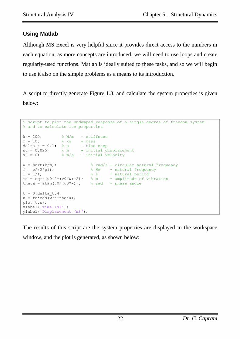
A script to directly generate Figure 1.3, and calculate the system properties is given
below:
% Script to plot the undamped response of a single degree of freedom system % and to calculate its properties
k = 100; % N/m - stiffness m = 10; % kg - mass delta_t = 0.1; % s - time step u0 = 0.025; % m - initial displacement v0 = 0; % m/s - initial velocity
w = sqrt(k/m); % rad/s - circular natural frequency f = w/(2*pi); % Hz - natural frequency T = 1/f; % s - natural period ro = sqrt(u0^2+(v0/w)^2); % m - amplitude of vibration theta = atan(v0/(u0*w)); % rad - phase angle
t = 0:delta_t:4; u = ro*cos(w*t-theta); plot(t,u); xlabel('Time (s)'); ylabel('Displacement (m)');
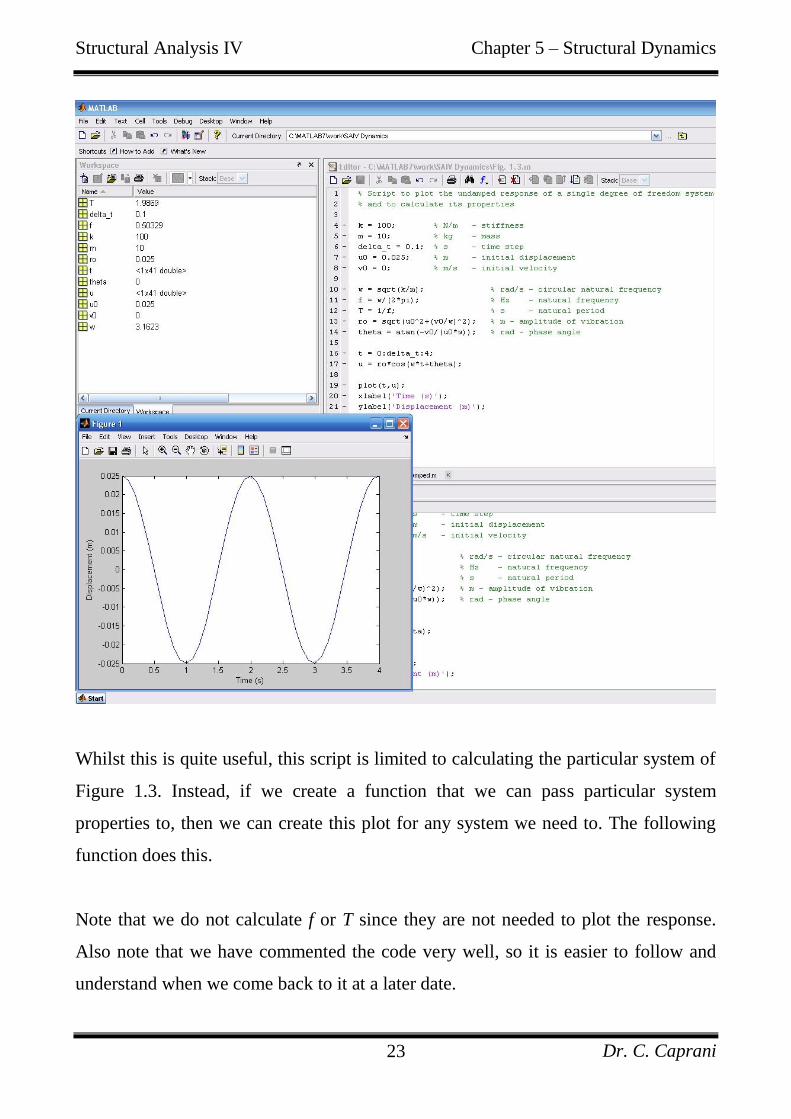
The results of this script are the system properties are displayed in the workspace
window, and the plot is generated, as shown below:
Structural Analysis IV Chapter 5 – Structural Dynamics
Dr. C. Caprani 23
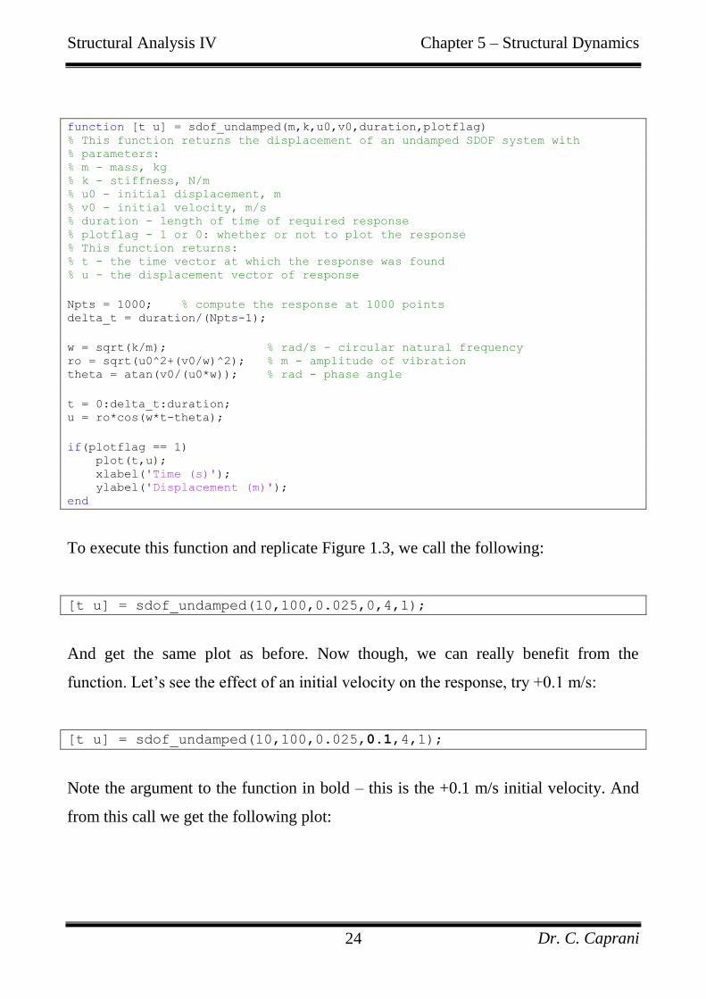
Whilst this is quite useful, this script is limited to calculating the particular system of
Figure 1.3. Instead, if we create a function that we can pass particular system
properties to, then we can create this plot for any system we need to. The following
function does this.
Note that we do not calculate f or T since they are not needed to plot the response.
Also note that we have commented the code very well, so it is easier to follow and
understand when we come back to it at a later date.
Structural Analysis IV Chapter 5 – Structural Dynamics
Dr. C. Caprani 24
function [t u] = sdof_undamped(m,k,u0,v0,duration,plotflag) % This function returns the displacement of an undamped SDOF system with % parameters: % m - mass, kg % k - stiffness, N/m % u0 - initial displacement, m % v0 - initial velocity, m/s % duration - length of time of required response % plotflag - 1 or 0: whether or not to plot the response % This function returns: % t - the time vector at which the response was found % u - the displacement vector of response
Npts = 1000; % compute the response at 1000 points delta_t = duration/(Npts-1);
w = sqrt(k/m); % rad/s - circular natural frequency ro = sqrt(u0^2+(v0/w)^2); % m - amplitude of vibration theta = atan(v0/(u0*w)); % rad - phase angle
t = 0:delta_t:duration; u = ro*cos(w*t-theta);
if(plotflag == 1) plot(t,u); xlabel('Time (s)'); ylabel('Displacement (m)'); end
To execute this function and replicate Figure 1.3, we call the following:
[t u] = sdof_undamped(10,100,0.025,0,4,1);
And get the same plot as before. Now though, we can really benefit from the
function. Let‟s see the effect of an initial velocity on the response, try +0.1 m/s:
[t u] = sdof_undamped(10,100,0.025,0.1,4,1);
Note the argument to the function in bold – this is the +0.1 m/s initial velocity. And
from this call we get the following plot:
Structural Analysis IV Chapter 5 – Structural Dynamics
Dr. C. Caprani 25
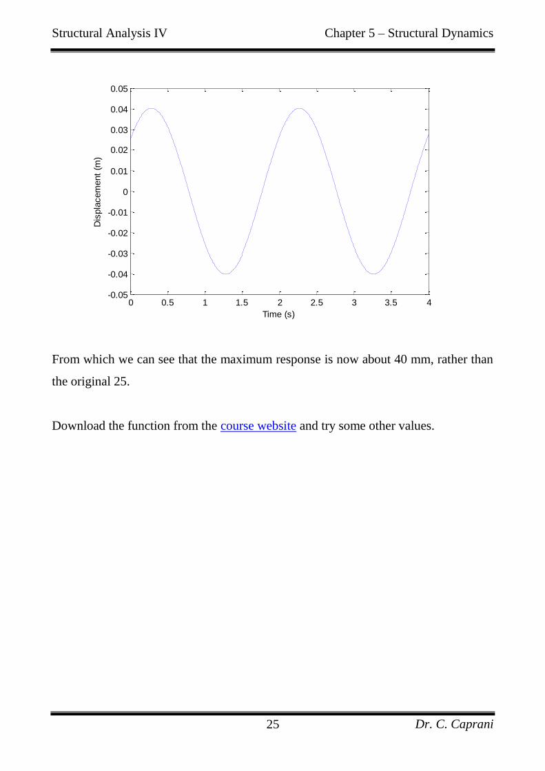
From which we can see that the maximum response is now about 40 mm, rather than
the original 25.
Download the function from the course website and try some other values.
0 0.5 1 1.5 2 2.5 3 3.5 4-0.05
-0.04
-0.03
-0.02
-0.01
0
0.01
0.02
0.03
0.04
0.05
Time (s)
Dis
pla
cem
ent
(m)
Structural Analysis IV Chapter 5 – Structural Dynamics
Dr. C. Caprani 26
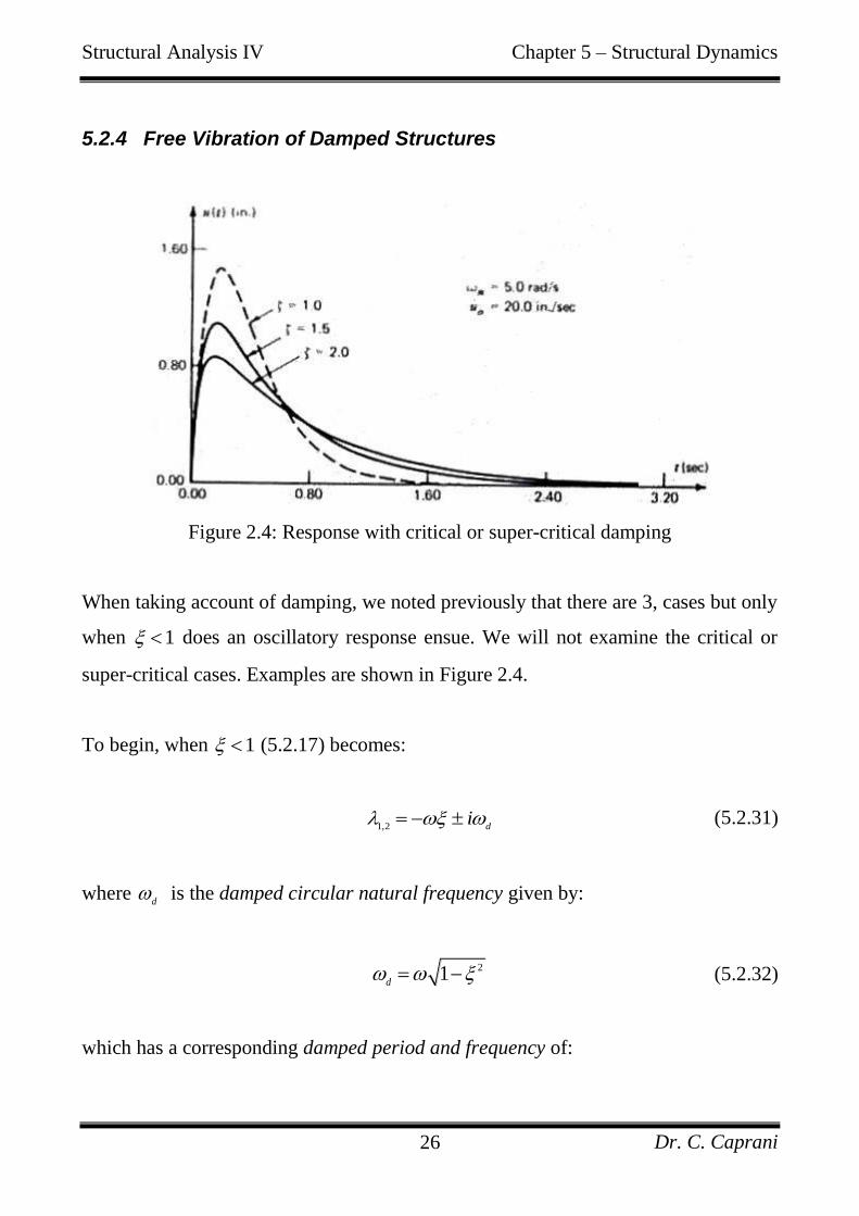
5.2.4 Free Vibration of Damped Structures
Figure 2.4: Response with critical or super-critical damping
When taking account of damping, we noted previously that there are 3, cases but only
when 1 does an oscillatory response ensue. We will not examine the critical or
super-critical cases. Examples are shown in Figure 2.4.
To begin, when 1 (5.2.17) becomes:
1,2 d
i (5.2.31)
where d
is the damped circular natural frequency given by:
21
d (5.2.32)
which has a corresponding damped period and frequency of:
Structural Analysis IV Chapter 5 – Structural Dynamics
Dr. C. Caprani 27
2
d
d
T
(5.2.33)
2
d
df
(5.2.34)
The general solution to equation (5.2.14), using Euler‟s formula again, becomes:
( ) cos sint
d du t e A t B t (5.2.35)
and again using the initial conditions we get:
0 0
0( ) cos sint d
d d
d
u uu t e u t t
(5.2.36)
Using the cosine addition rule again we also have:
( ) cost
du t e t (5.2.37)
In which
2
2 0 0
0
d
u uu
(5.2.38)
0 0
0
tand
u u
u
(5.2.39)
Equations (5.2.35) to (5.2.39) correspond to those of the undamped case looked at
previously when 0 .
Structural Analysis IV Chapter 5 – Structural Dynamics
Dr. C. Caprani 28
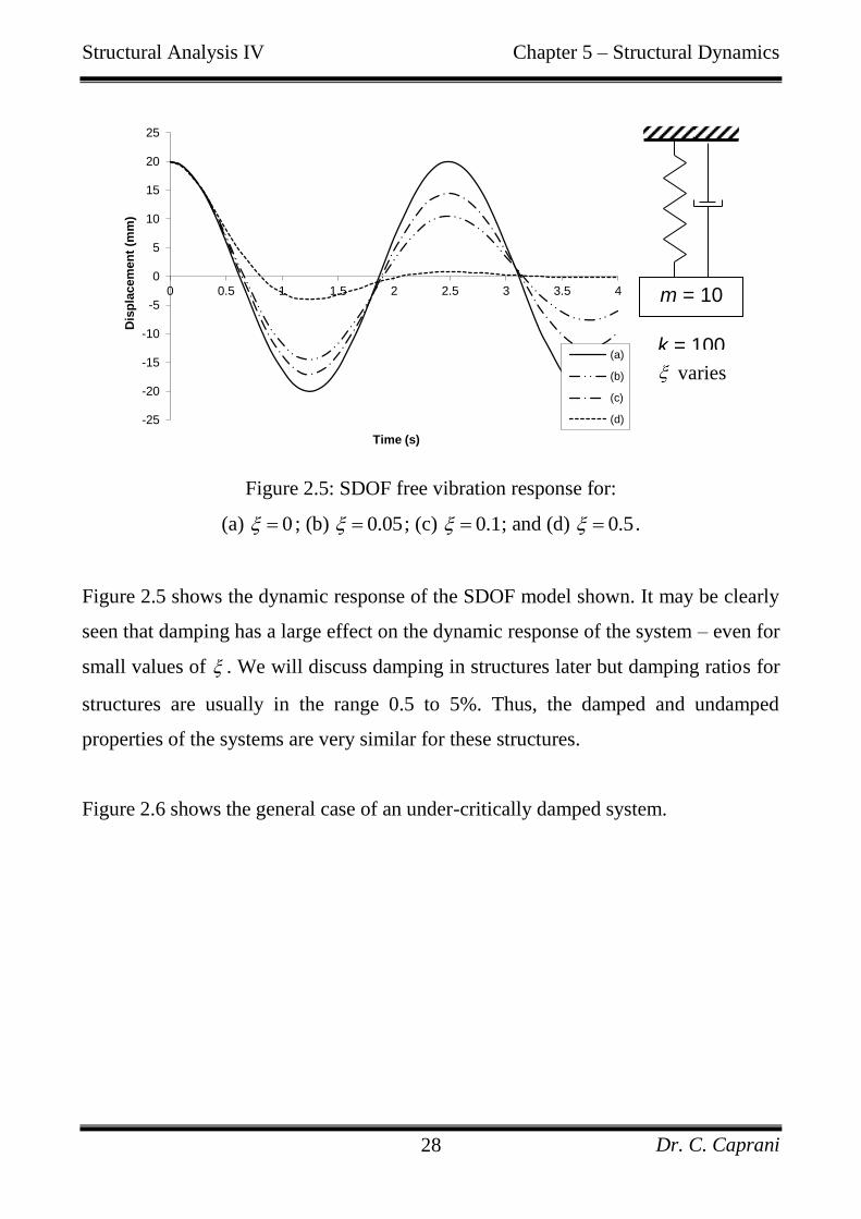
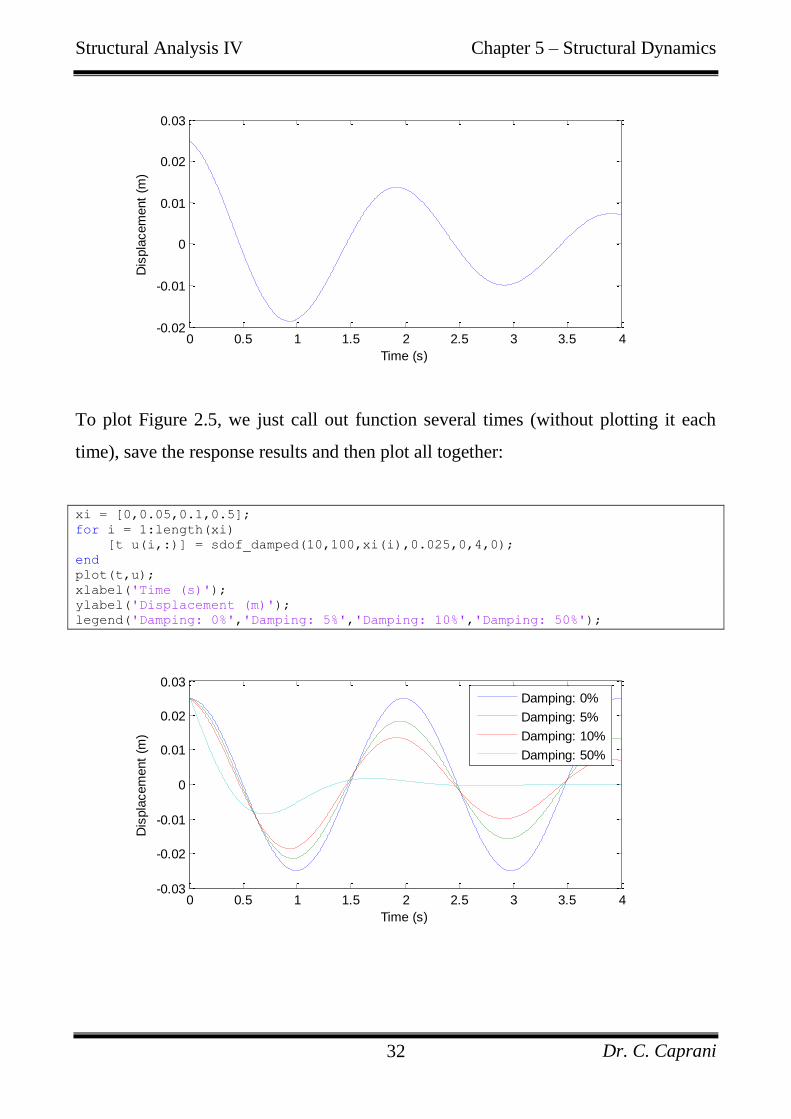
Figure 2.5: SDOF free vibration response for:
(a) 0 ; (b) 0.05 ; (c) 0.1 ; and (d) 0.5 .
Figure 2.5 shows the dynamic response of the SDOF model shown. It may be clearly
seen that damping has a large effect on the dynamic response of the system – even for
small values of . We will discuss damping in structures later but damping ratios for
structures are usually in the range 0.5 to 5%. Thus, the damped and undamped
properties of the systems are very similar for these structures.
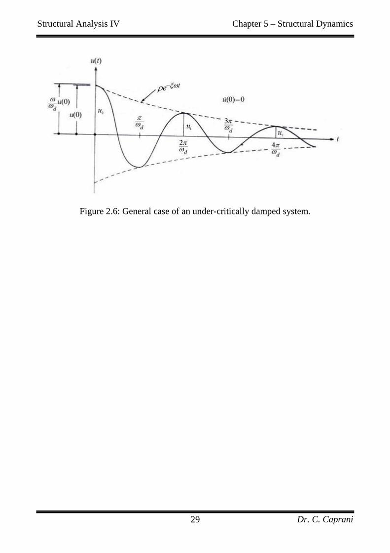
Figure 2.6 shows the general case of an under-critically damped system.
-25
-20
-15
-10
-5
0
5
10
15
20
25
0 0.5 1 1.5 2 2.5 3 3.5 4
Dis
pla
cem
en
t (m
m)
Time (s)
(a)
(b)
(c)
(d)
m = 10
k = 100
varies
Structural Analysis IV Chapter 5 – Structural Dynamics
Dr. C. Caprani 29
Figure 2.6: General case of an under-critically damped system.
Structural Analysis IV Chapter 5 – Structural Dynamics
Dr. C. Caprani 30
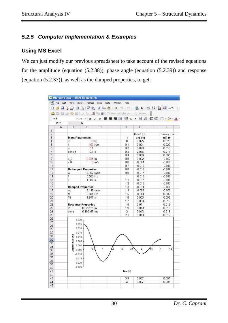
5.2.5 Computer Implementation & Examples
Using MS Excel
We can just modify our previous spreadsheet to take account of the revised equations
for the amplitude (equation (5.2.38)), phase angle (equation (5.2.39)) and response
(equation (5.2.37)), as well as the damped properties, to get:
Structural Analysis IV Chapter 5 – Structural Dynamics
Dr. C. Caprani 31
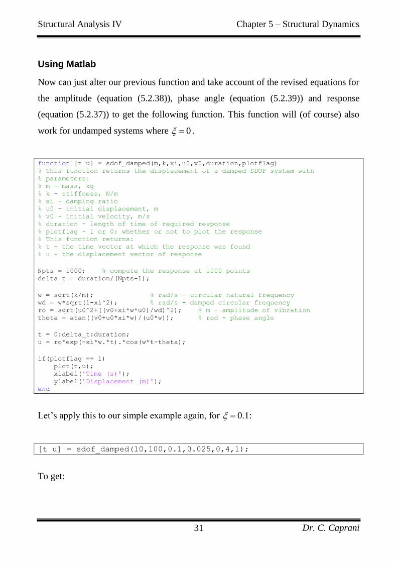
Using Matlab
Now can just alter our previous function and take account of the revised equations for
the amplitude (equation (5.2.38)), phase angle (equation (5.2.39)) and response
(equation (5.2.37)) to get the following function. This function will (of course) also
work for undamped systems where 0 .
function [t u] = sdof_damped(m,k,xi,u0,v0,duration,plotflag) % This function returns the displacement of a damped SDOF system with % parameters: % m - mass, kg % k - stiffness, N/m % xi - damping ratio % u0 - initial displacement, m % v0 - initial velocity, m/s % duration - length of time of required response % plotflag - 1 or 0: whether or not to plot the response % This function returns: % t - the time vector at which the response was found % u - the displacement vector of response
Npts = 1000; % compute the response at 1000 points delta_t = duration/(Npts-1);
w = sqrt(k/m); % rad/s - circular natural frequency wd = w*sqrt(1-xi^2); % rad/s - damped circular frequency ro = sqrt(u0^2+((v0+xi*w*u0)/wd)^2); % m - amplitude of vibration theta = atan((v0+u0*xi*w)/(u0*w)); % rad - phase angle
t = 0:delta_t:duration; u = ro*exp(-xi*w.*t).*cos(w*t-theta);
if(plotflag == 1) plot(t,u); xlabel('Time (s)'); ylabel('Displacement (m)'); end
Let‟s apply this to our simple example again, for 0.1 :
[t u] = sdof_damped(10,100,0.1,0.025,0,4,1);
To get:
Structural Analysis IV Chapter 5 – Structural Dynamics
Dr. C. Caprani 32
To plot Figure 2.5, we just call out function several times (without plotting it each
time), save the response results and then plot all together:
xi = [0,0.05,0.1,0.5]; for i = 1:length(xi) [t u(i,:)] = sdof_damped(10,100,xi(i),0.025,0,4,0); end plot(t,u); xlabel('Time (s)'); ylabel('Displacement (m)'); legend('Damping: 0%','Damping: 5%','Damping: 10%','Damping: 50%');
0 0.5 1 1.5 2 2.5 3 3.5 4-0.02
-0.01
0
0.01
0.02
0.03
Time (s)
Dis
pla
cem
ent
(m)
0 0.5 1 1.5 2 2.5 3 3.5 4-0.03
-0.02
-0.01
0
0.01
0.02
0.03
Time (s)
Dis
pla
cem
ent
(m)
Damping: 0%
Damping: 5%
Damping: 10%
Damping: 50%
Structural Analysis IV Chapter 5 – Structural Dynamics
Dr. C. Caprani 33
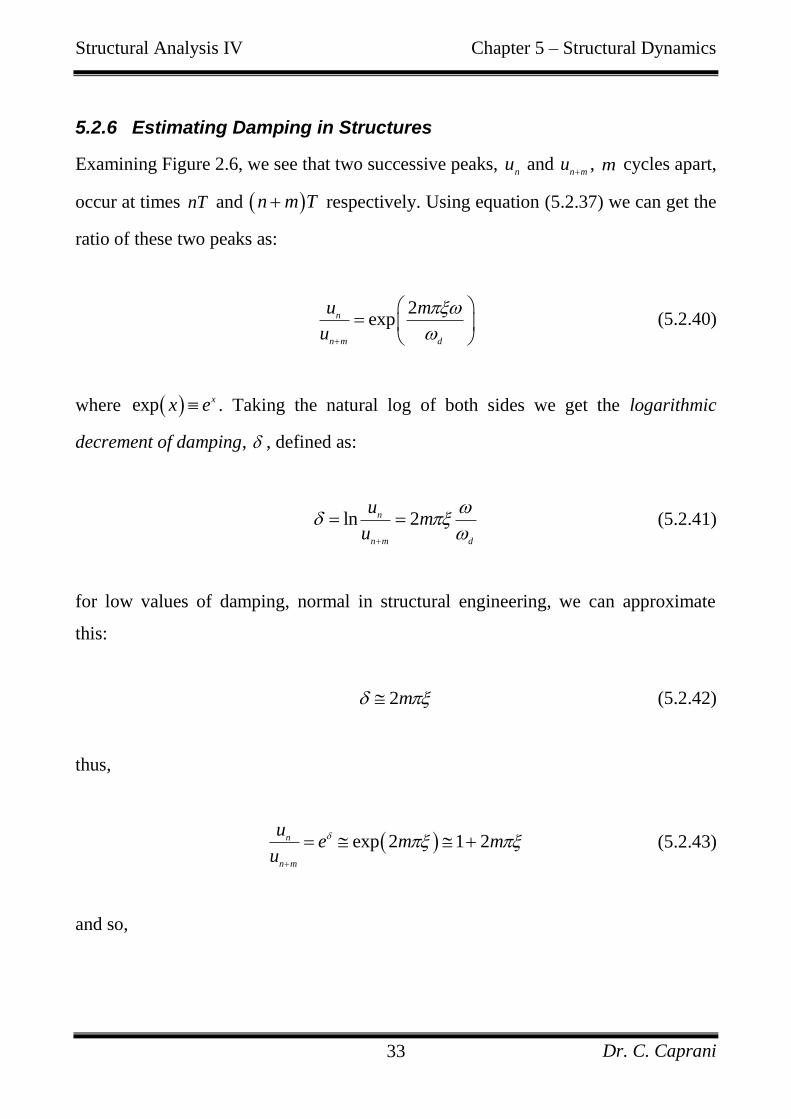
5.2.6 Estimating Damping in Structures
Examining Figure 2.6, we see that two successive peaks, n
u and n m
u
, m cycles apart,
occur at times nT and n m T respectively. Using equation (5.2.37) we can get the
ratio of these two peaks as:
2
expn
n m d
u m
u
(5.2.40)
where exp xx e . Taking the natural log of both sides we get the logarithmic
decrement of damping, , defined as:
ln 2n
n m d
um
u
(5.2.41)
for low values of damping, normal in structural engineering, we can approximate
this:
2m (5.2.42)
thus,
exp 2 1 2n
n m
ue m m
u
(5.2.43)
and so,
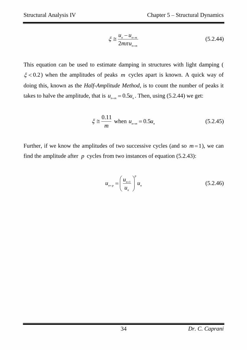
Structural Analysis IV Chapter 5 – Structural Dynamics
Dr. C. Caprani 34
2
n n m
n m
u u
m u
(5.2.44)
This equation can be used to estimate damping in structures with light damping (
0.2 ) when the amplitudes of peaks m cycles apart is known. A quick way of
doing this, known as the Half-Amplitude Method, is to count the number of peaks it
takes to halve the amplitude, that is 0.5n m n
u u . Then, using (5.2.44) we get:
0.11
m when 0.5
n m nu u
(5.2.45)
Further, if we know the amplitudes of two successive cycles (and so 1m ), we can
find the amplitude after p cycles from two instances of equation (5.2.43):
1
p
n
n p n
n
uu u
u
(5.2.46)
Structural Analysis IV Chapter 5 – Structural Dynamics
Dr. C. Caprani 35
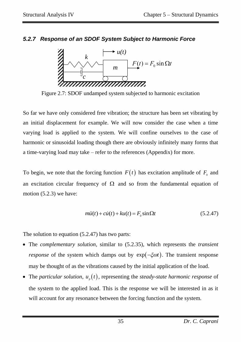
5.2.7 Response of an SDOF System Subject to Harmonic Force
Figure 2.7: SDOF undamped system subjected to harmonic excitation
So far we have only considered free vibration; the structure has been set vibrating by
an initial displacement for example. We will now consider the case when a time
varying load is applied to the system. We will confine ourselves to the case of
harmonic or sinusoidal loading though there are obviously infinitely many forms that
a time-varying load may take – refer to the references (Appendix) for more.
To begin, we note that the forcing function F t has excitation amplitude of 0
F and
an excitation circular frequency of and so from the fundamental equation of
motion (5.2.3) we have:
0
( ) ( ) ( ) sinmu t cu t ku t F t (5.2.47)
The solution to equation (5.2.47) has two parts:
The complementary solution, similar to (5.2.35), which represents the transient
response of the system which damps out by exp t . The transient response
may be thought of as the vibrations caused by the initial application of the load.
The particular solution, pu t , representing the steady-state harmonic response of
the system to the applied load. This is the response we will be interested in as it
will account for any resonance between the forcing function and the system.
m
k u(t)
c
Structural Analysis IV Chapter 5 – Structural Dynamics
Dr. C. Caprani 36
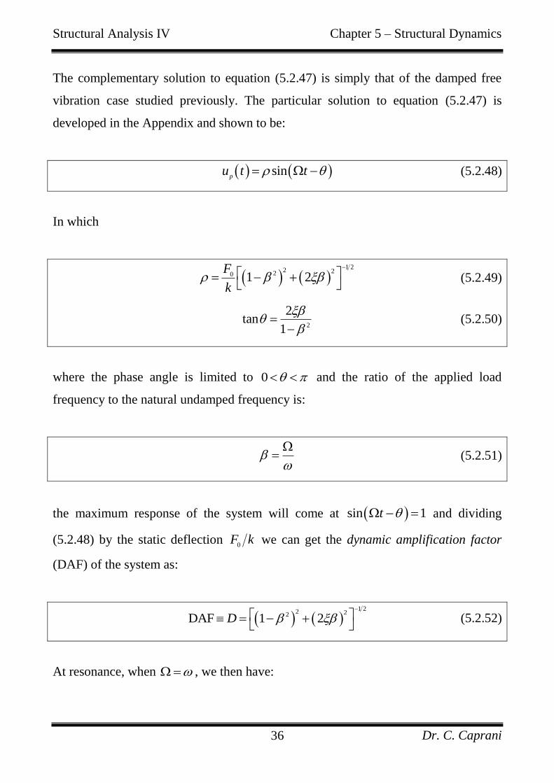
The complementary solution to equation (5.2.47) is simply that of the damped free
vibration case studied previously. The particular solution to equation (5.2.47) is
developed in the Appendix and shown to be:
sinp
u t t (5.2.48)
In which
1 2
2 220 1 2F
k
(5.2.49)
2
2tan
1
(5.2.50)
where the phase angle is limited to 0 and the ratio of the applied load
frequency to the natural undamped frequency is:
(5.2.51)
the maximum response of the system will come at sin 1t and dividing
(5.2.48) by the static deflection 0
F k we can get the dynamic amplification factor
(DAF) of the system as:
1 2
2 22DAF 1 2D
(5.2.52)
At resonance, when , we then have:
Structural Analysis IV Chapter 5 – Structural Dynamics
Dr. C. Caprani 37
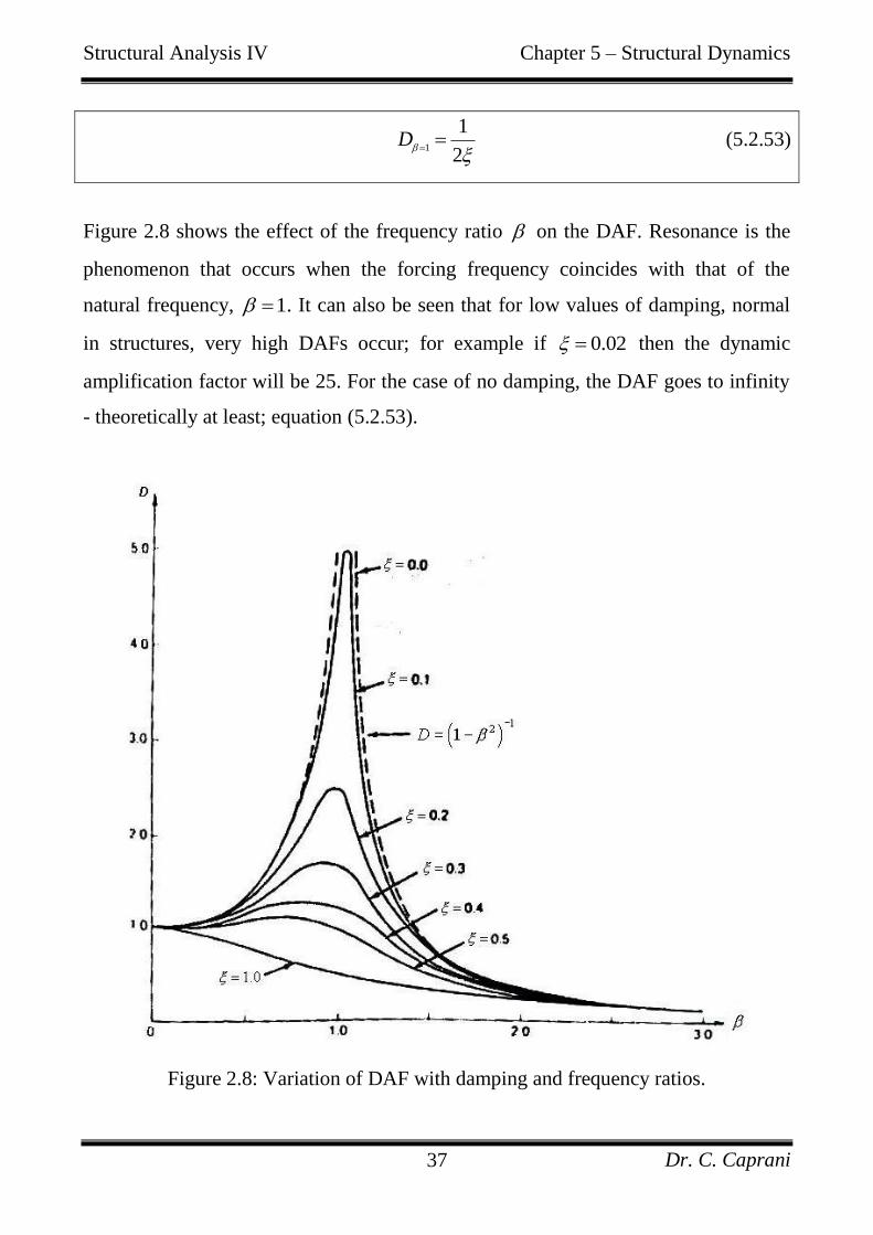
1
1
2D
(5.2.53)
Figure 2.8 shows the effect of the frequency ratio on the DAF. Resonance is the
phenomenon that occurs when the forcing frequency coincides with that of the
natural frequency, 1 . It can also be seen that for low values of damping, normal
in structures, very high DAFs occur; for example if 0.02 then the dynamic
amplification factor will be 25. For the case of no damping, the DAF goes to infinity
- theoretically at least; equation (5.2.53).
Figure 2.8: Variation of DAF with damping and frequency ratios.
Structural Analysis IV Chapter 5 – Structural Dynamics
Dr. C. Caprani 38
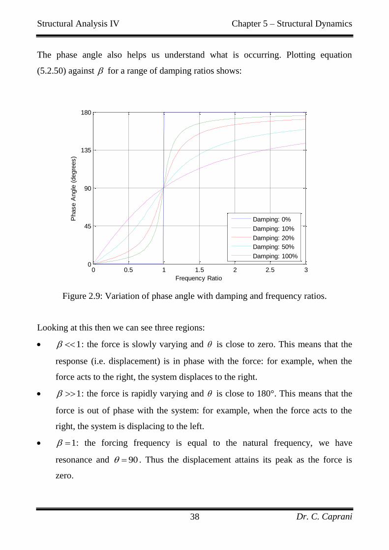
The phase angle also helps us understand what is occurring. Plotting equation
(5.2.50) against for a range of damping ratios shows:
Figure 2.9: Variation of phase angle with damping and frequency ratios.
Looking at this then we can see three regions:
1 : the force is slowly varying and is close to zero. This means that the
response (i.e. displacement) is in phase with the force: for example, when the
force acts to the right, the system displaces to the right.
1 : the force is rapidly varying and is close to 180°. This means that the
force is out of phase with the system: for example, when the force acts to the
right, the system is displacing to the left.
1 : the forcing frequency is equal to the natural frequency, we have
resonance and 90 . Thus the displacement attains its peak as the force is
zero.
0 0.5 1 1.5 2 2.5 30
45
90
135
180
Frequency Ratio
Phase A
ngle
(degre
es)
Damping: 0%
Damping: 10%
Damping: 20%
Damping: 50%
Damping: 100%
Structural Analysis IV Chapter 5 – Structural Dynamics
Dr. C. Caprani 39
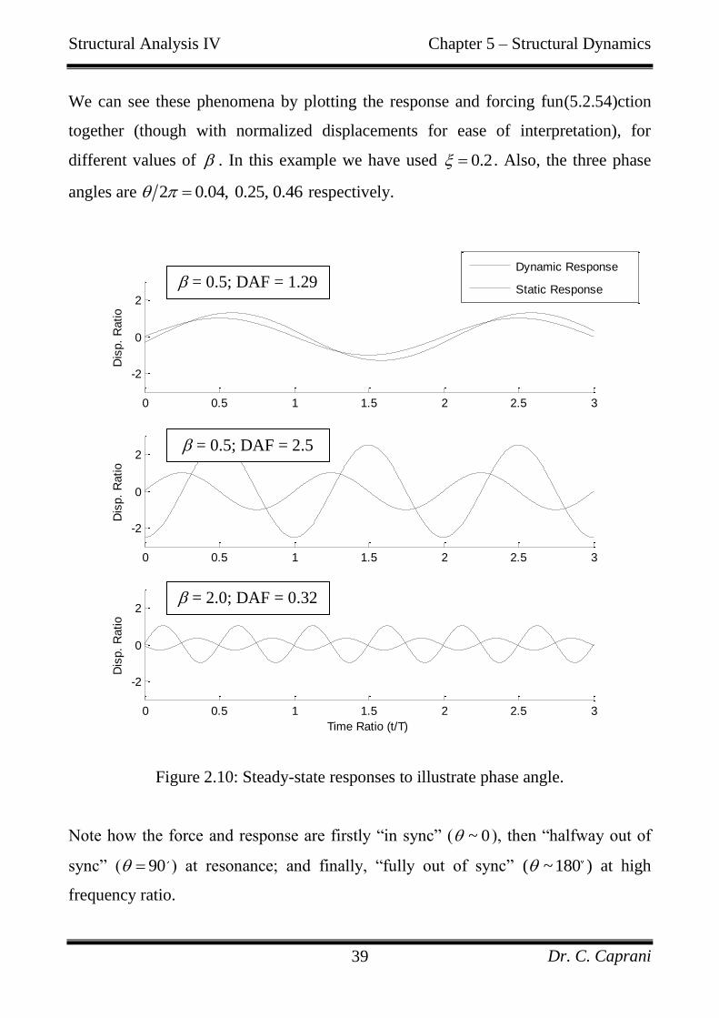
We can see these phenomena by plotting the response and forcing fun(5.2.54)ction
together (though with normalized displacements for ease of interpretation), for
different values of . In this example we have used 0.2 . Also, the three phase
angles are 2 0.04, 0.25, 0.46 respectively.
Figure 2.10: Steady-state responses to illustrate phase angle.
Note how the force and response are firstly “in sync” ( ~ 0 ), then “halfway out of
sync” ( 90 ) at resonance; and finally, “fully out of sync” ( ~180 ) at high
frequency ratio.
0 0.5 1 1.5 2 2.5 3
-2
0
2
Dis
p.
Ratio
0 0.5 1 1.5 2 2.5 3
-2
0
2
Dis
p.
Ratio
0 0.5 1 1.5 2 2.5 3
-2
0
2
Dis
p.
Ratio
Time Ratio (t/T)
Dynamic Response
Static Response = 0.5; DAF = 1.29
= 0.5; DAF = 2.5
= 2.0; DAF = 0.32
Structural Analysis IV Chapter 5 – Structural Dynamics
Dr. C. Caprani 40
Maximum Steady-State Displacement
The maximum steady-state displacement occurs when the DAF is a maximum. This
occurs when the denominator of equation (5.2.52) is a minimum:
1 22 22
2 2
2 22
2 2
0
1 2 0
4 1 4 210
2 1 2
1 2 0
d D
d
d
d
The trivial solution to this equation of 0 corresponds to an applied forcing
function that has zero frequency –the static loading effect of the forcing function. The
other solution is:
21 2 (5.2.54)
Which for low values of damping, 0.1 approximately, is very close to unity. The
corresponding maximum DAF is then given by substituting (5.2.54) into equation
(5.2.52) to get:
max 2
1
2 1D
(5.2.55)
Which reduces to equation (5.2.53) for 1 , as it should.
Structural Analysis IV Chapter 5 – Structural Dynamics
Dr. C. Caprani 41
Measurement of Natural Frequencies
It may be seen from equation (5.2.50) that when 1 , 2 ; this phase
relationship allows the accurate measurements of the natural frequencies of
structures. That is, we change the input frequency in small increments until we can
identify a peak response: the value of at the peak response is then the natural
frequency of the system. Example 2.1 gave the natural frequency based on this type
of test.
Structural Analysis IV Chapter 5 – Structural Dynamics
Dr. C. Caprani 42
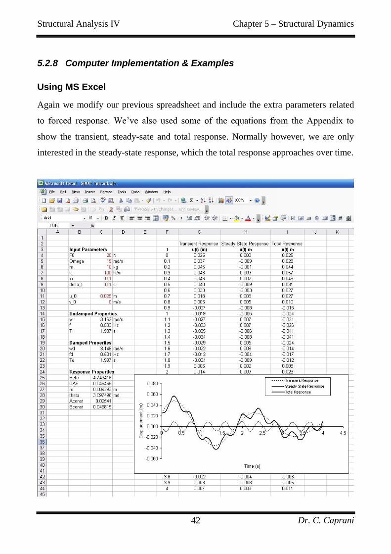
5.2.8 Computer Implementation & Examples
Using MS Excel
Again we modify our previous spreadsheet and include the extra parameters related
to forced response. We‟ve also used some of the equations from the Appendix to
show the transient, steady-sate and total response. Normally however, we are only
interested in the steady-state response, which the total response approaches over time.
Structural Analysis IV Chapter 5 – Structural Dynamics
Dr. C. Caprani 43
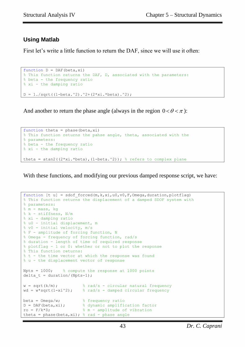
Using Matlab
First let‟s write a little function to return the DAF, since we will use it often:
function D = DAF(beta,xi) % This function returns the DAF, D, associated with the parameters: % beta - the frequency ratio % xi - the damping ratio
D = 1./sqrt((1-beta.^2).^2+(2*xi.*beta).^2);
And another to return the phase angle (always in the region 0 ):
function theta = phase(beta,xi) % This function returns the pahse angle, theta, associated with the % parameters: % beta - the frequency ratio % xi - the damping ratio
theta = atan2((2*xi.*beta),(1-beta.^2)); % refers to complex plane
With these functions, and modifying our previous damped response script, we have:
function [t u] = sdof_forced(m,k,xi,u0,v0,F,Omega,duration,plotflag) % This function returns the displacement of a damped SDOF system with % parameters: % m - mass, kg % k - stiffness, N/m % xi - damping ratio % u0 - initial displacement, m % v0 - initial velocity, m/s % F - amplitude of forcing function, N % Omega - frequency of forcing function, rad/s % duration - length of time of required response % plotflag - 1 or 0: whether or not to plot the response % This function returns: % t - the time vector at which the response was found % u - the displacement vector of response
Npts = 1000; % compute the response at 1000 points delta_t = duration/(Npts-1);
w = sqrt(k/m); % rad/s - circular natural frequency wd = w*sqrt(1-xi^2); % rad/s - damped circular frequency
beta = Omega/w; % frequency ratio D = DAF(beta,xi); % dynamic amplification factor ro = F/k*D; % m - amplitude of vibration theta = phase(beta,xi); % rad - phase angle
Structural Analysis IV Chapter 5 – Structural Dynamics
Dr. C. Caprani 44
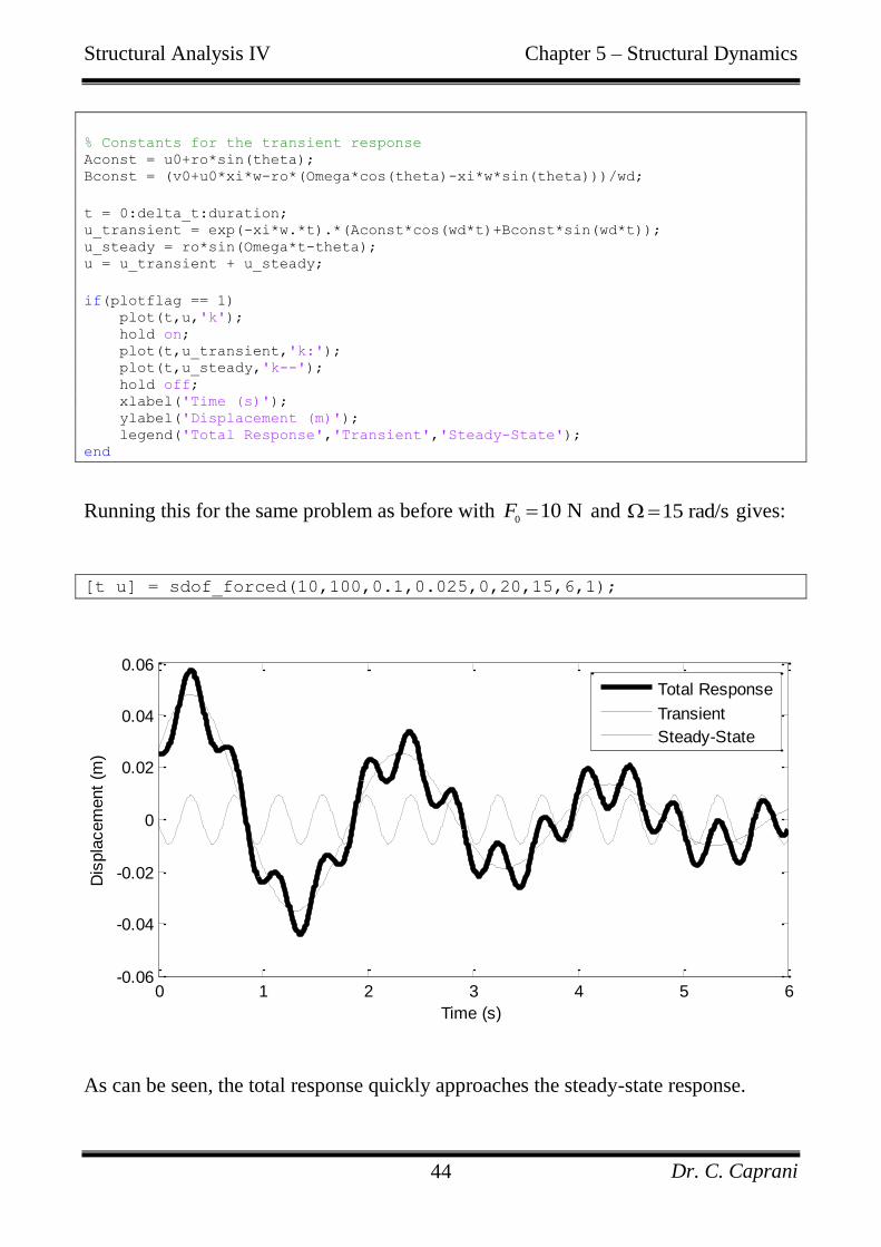
% Constants for the transient response Aconst = u0+ro*sin(theta); Bconst = (v0+u0*xi*w-ro*(Omega*cos(theta)-xi*w*sin(theta)))/wd;
t = 0:delta_t:duration; u_transient = exp(-xi*w.*t).*(Aconst*cos(wd*t)+Bconst*sin(wd*t)); u_steady = ro*sin(Omega*t-theta); u = u_transient + u_steady;
if(plotflag == 1) plot(t,u,'k'); hold on; plot(t,u_transient,'k:'); plot(t,u_steady,'k--'); hold off; xlabel('Time (s)'); ylabel('Displacement (m)'); legend('Total Response','Transient','Steady-State'); end
Running this for the same problem as before with 0
10 NF and 15 rad/s gives:
[t u] = sdof_forced(10,100,0.1,0.025,0,20,15,6,1);
As can be seen, the total response quickly approaches the steady-state response.
0 1 2 3 4 5 6-0.06
-0.04
-0.02
0
0.02
0.04
0.06
Time (s)
Dis
pla
cem
ent
(m)
Total Response
Transient
Steady-State
Structural Analysis IV Chapter 5 – Structural Dynamics
Dr. C. Caprani 45
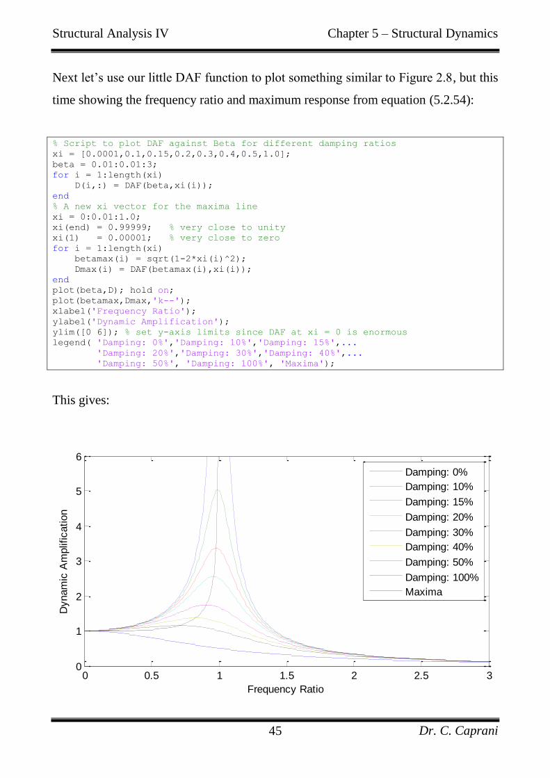
Next let‟s use our little DAF function to plot something similar to Figure 2.8, but this
time showing the frequency ratio and maximum response from equation (5.2.54):
% Script to plot DAF against Beta for different damping ratios xi = [0.0001,0.1,0.15,0.2,0.3,0.4,0.5,1.0]; beta = 0.01:0.01:3; for i = 1:length(xi) D(i,:) = DAF(beta,xi(i)); end % A new xi vector for the maxima line xi = 0:0.01:1.0; xi(end) = 0.99999; % very close to unity xi(1) = 0.00001; % very close to zero for i = 1:length(xi) betamax(i) = sqrt(1-2*xi(i)^2); Dmax(i) = DAF(betamax(i),xi(i)); end plot(beta,D); hold on; plot(betamax,Dmax,'k--'); xlabel('Frequency Ratio'); ylabel('Dynamic Amplification'); ylim([0 6]); % set y-axis limits since DAF at xi = 0 is enormous legend( 'Damping: 0%','Damping: 10%','Damping: 15%',... 'Damping: 20%','Damping: 30%','Damping: 40%',... 'Damping: 50%', 'Damping: 100%', 'Maxima');
This gives:
0 0.5 1 1.5 2 2.5 30
1
2
3
4
5
6
Frequency Ratio
Dynam
ic A
mplif
ication
Damping: 0%
Damping: 10%
Damping: 15%
Damping: 20%
Damping: 30%
Damping: 40%
Damping: 50%
Damping: 100%
Maxima
Structural Analysis IV Chapter 5 – Structural Dynamics
Dr. C. Caprani 46
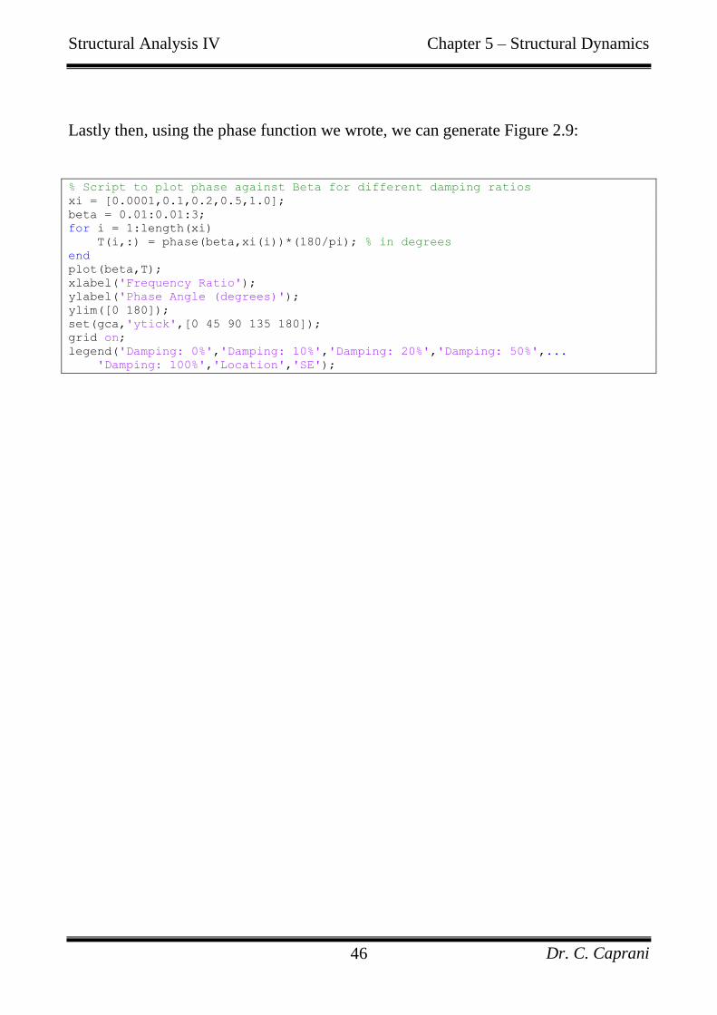
Lastly then, using the phase function we wrote, we can generate Figure 2.9:
% Script to plot phase against Beta for different damping ratios xi = [0.0001,0.1,0.2,0.5,1.0]; beta = 0.01:0.01:3; for i = 1:length(xi) T(i,:) = phase(beta,xi(i))*(180/pi); % in degrees end plot(beta,T); xlabel('Frequency Ratio'); ylabel('Phase Angle (degrees)'); ylim([0 180]); set(gca,'ytick',[0 45 90 135 180]); grid on; legend('Damping: 0%','Damping: 10%','Damping: 20%','Damping: 50%',... 'Damping: 100%','Location','SE');
Structural Analysis IV Chapter 5 – Structural Dynamics
Dr. C. Caprani 47
5.2.9 Numerical Integration – Newmark’s Method
Introduction
The loading that can be applied to a structure is infinitely variable and closed-form
mathematical solutions can only be achieved for a small number of cases. For
arbitrary excitation we must resort to computational methods, which aim to solve the
basic structural dynamics equation, at the next time-step:
1 1 1 1i i i i
mu cu ku F (5.2.56)
There are three basic time-stepping approaches to the solution of the structural
dynamics equations:
1. Interpolation of the excitation function;
2. Use of finite differences of velocity and acceleration;
3. An assumed variation of acceleration.
We will examine one method from the third category only. However, it is an
important method and is extensible to non-linear systems, as well as multi degree-of-
freedom systems (MDOF).
Structural Analysis IV Chapter 5 – Structural Dynamics
Dr. C. Caprani 48
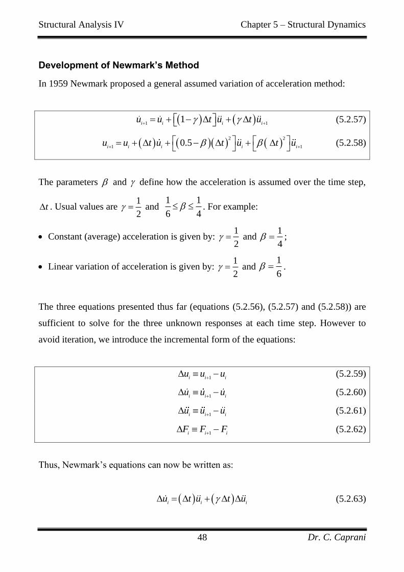
Development of Newmark’s Method
In 1959 Newmark proposed a general assumed variation of acceleration method:
1 11
i i i iu u t u t u
(5.2.57)
2 2
1 10.5
i i i i iu u t u t u t u
(5.2.58)
The parameters and define how the acceleration is assumed over the time step,
t . Usual values are 1
2 and
1 1
6 4 . For example:
Constant (average) acceleration is given by: 1
2 and
1
4 ;
Linear variation of acceleration is given by: 1
2 and
1
6 .
The three equations presented thus far (equations (5.2.56), (5.2.57) and (5.2.58)) are
sufficient to solve for the three unknown responses at each time step. However to
avoid iteration, we introduce the incremental form of the equations:
1i i i
u u u
(5.2.59)
1i i i
u u u
(5.2.60)
1i i i
u u u
(5.2.61)
1i i i
F F F
(5.2.62)
Thus, Newmark‟s equations can now be written as:
i i iu t u t u (5.2.63)
Structural Analysis IV Chapter 5 – Structural Dynamics
Dr. C. Caprani 49
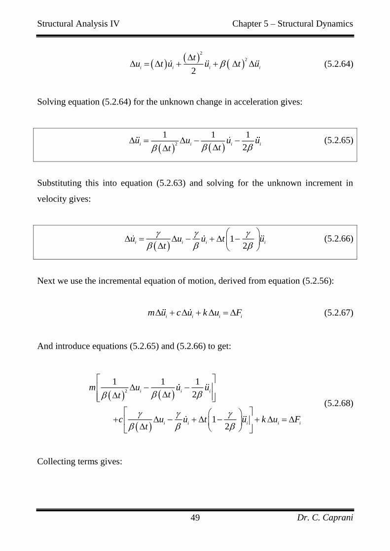
2
2
2i i i i
tu t u u t u
(5.2.64)
Solving equation (5.2.64) for the unknown change in acceleration gives:
2
1 1 1
2i i i i
u u u utt
(5.2.65)
Substituting this into equation (5.2.63) and solving for the unknown increment in
velocity gives:
12
i i i iu u u t u
t
(5.2.66)
Next we use the incremental equation of motion, derived from equation (5.2.56):
i i i i
m u c u k u F (5.2.67)
And introduce equations (5.2.65) and (5.2.66) to get:
2
1 1 1
2
12
i i i
i i i i i
m u u utt
c u u t u k u Ft
(5.2.68)
Collecting terms gives:
Structural Analysis IV Chapter 5 – Structural Dynamics
Dr. C. Caprani 50
2
1
1 11
2 2
i
i i i
m c k utt
F m c u m t c ut
(5.2.69)
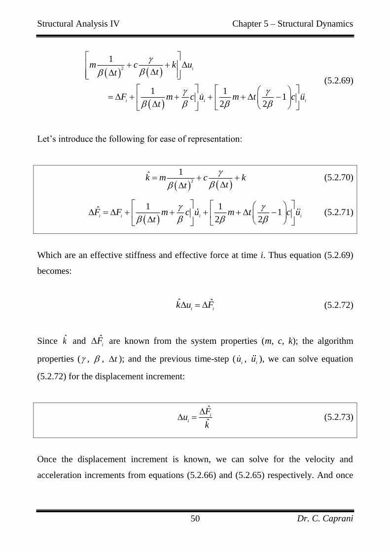
Let‟s introduce the following for ease of representation:
2
1k̂ m c k
tt
(5.2.70)
1 1ˆ 1
2 2i i i i
F F m c u m t c ut
(5.2.71)
Which are an effective stiffness and effective force at time i. Thus equation (5.2.69)
becomes:
ˆ ˆi i
k u F (5.2.72)
Since k̂ and ˆi
F are known from the system properties (m, c, k); the algorithm
properties ( , , t ); and the previous time-step (i
u , i
u ), we can solve equation
(5.2.72) for the displacement increment:
ˆ
ˆi
i
Fu
k
(5.2.73)
Once the displacement increment is known, we can solve for the velocity and
acceleration increments from equations (5.2.66) and (5.2.65) respectively. And once
Structural Analysis IV Chapter 5 – Structural Dynamics
Dr. C. Caprani 51
all the increments are known we can compute the properties at the current time-step
by just adding to the values at the previous time-step, equations (5.2.59) to (5.2.61).
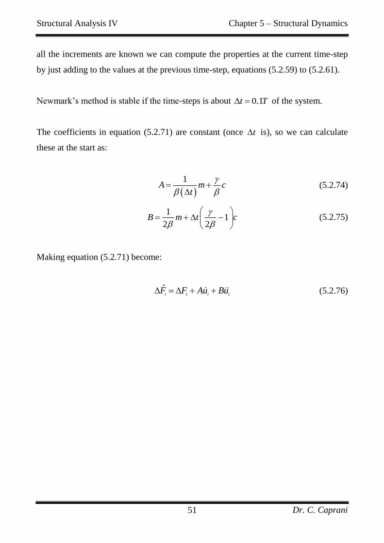
Newmark‟s method is stable if the time-steps is about 0.1t T of the system.
The coefficients in equation (5.2.71) are constant (once t is), so we can calculate
these at the start as:
1
A m ct
(5.2.74)
1
12 2
B m t c
(5.2.75)
Making equation (5.2.71) become:
ˆi i i i
F F Au Bu (5.2.76)
Structural Analysis IV Chapter 5 – Structural Dynamics
Dr. C. Caprani 52
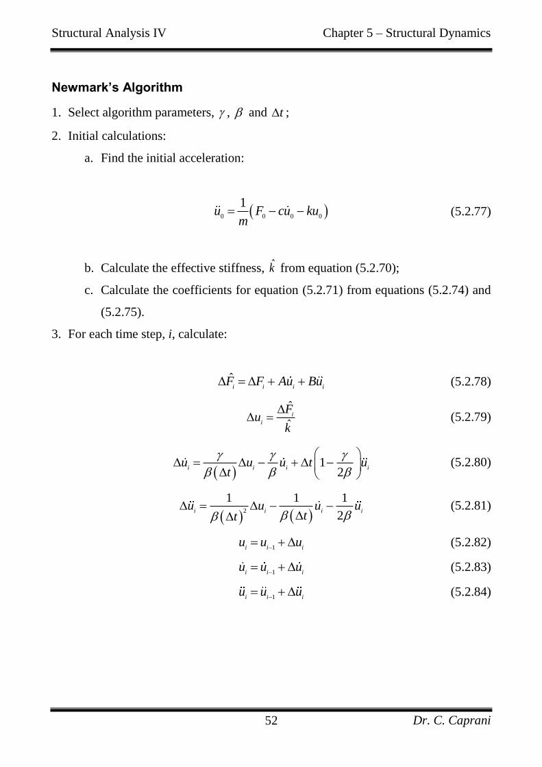
Newmark’s Algorithm
1. Select algorithm parameters, , and t ;
2. Initial calculations:
a. Find the initial acceleration:
0 0 0 0
1u F cu ku
m (5.2.77)
b. Calculate the effective stiffness, k̂ from equation (5.2.70);
c. Calculate the coefficients for equation (5.2.71) from equations (5.2.74) and
(5.2.75).
3. For each time step, i, calculate:
ˆi i i i
F F Au Bu (5.2.78)
ˆ
ˆi
i
Fu
k
(5.2.79)
12
i i i iu u u t u
t
(5.2.80)
2
1 1 1
2i i i i
u u u utt
(5.2.81)
1i i i
u u u
(5.2.82)
1i i i
u u u
(5.2.83)
1i i i
u u u
(5.2.84)
Structural Analysis IV Chapter 5 – Structural Dynamics
Dr. C. Caprani 53
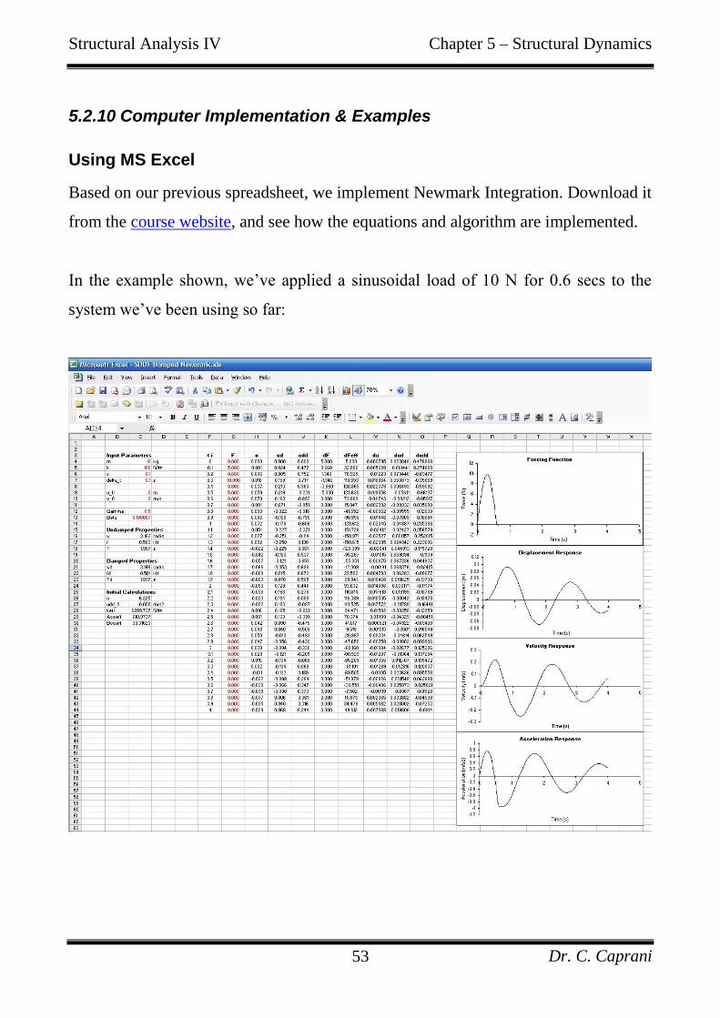
5.2.10 Computer Implementation & Examples
Using MS Excel
Based on our previous spreadsheet, we implement Newmark Integration. Download it
from the course website, and see how the equations and algorithm are implemented.
In the example shown, we‟ve applied a sinusoidal load of 10 N for 0.6 secs to the
system we‟ve been using so far:
Structural Analysis IV Chapter 5 – Structural Dynamics
Dr. C. Caprani 54
Using Matlab
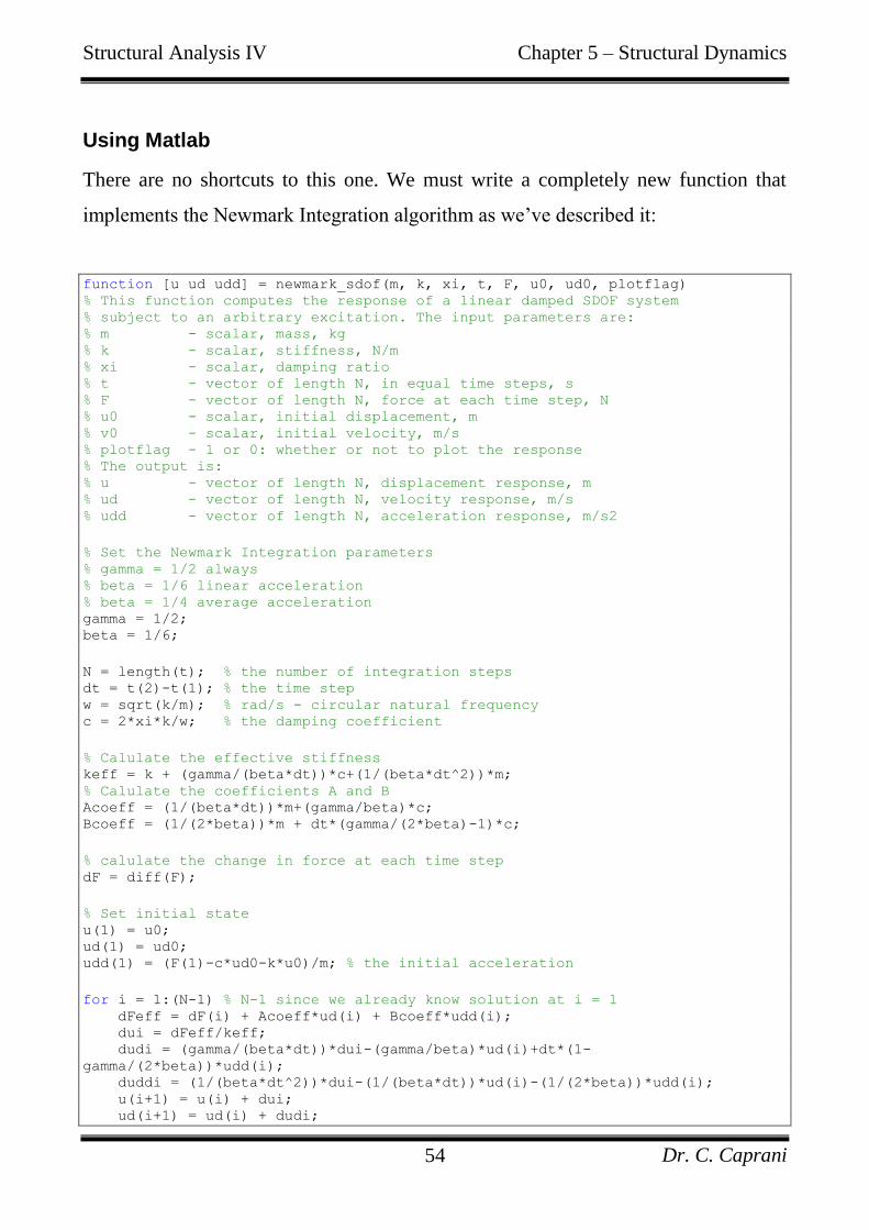
There are no shortcuts to this one. We must write a completely new function that
implements the Newmark Integration algorithm as we‟ve described it:
function [u ud udd] = newmark_sdof(m, k, xi, t, F, u0, ud0, plotflag) % This function computes the response of a linear damped SDOF system % subject to an arbitrary excitation. The input parameters are: % m - scalar, mass, kg % k - scalar, stiffness, N/m % xi - scalar, damping ratio % t - vector of length N, in equal time steps, s % F - vector of length N, force at each time step, N % u0 - scalar, initial displacement, m % v0 - scalar, initial velocity, m/s % plotflag - 1 or 0: whether or not to plot the response % The output is: % u - vector of length N, displacement response, m % ud - vector of length N, velocity response, m/s % udd - vector of length N, acceleration response, m/s2
% Set the Newmark Integration parameters % gamma = 1/2 always % beta = 1/6 linear acceleration % beta = 1/4 average acceleration gamma = 1/2; beta = 1/6;
N = length(t); % the number of integration steps dt = t(2)-t(1); % the time step w = sqrt(k/m); % rad/s - circular natural frequency c = 2*xi*k/w; % the damping coefficient
% Calulate the effective stiffness keff = k + (gamma/(beta*dt))*c+(1/(beta*dt^2))*m; % Calulate the coefficients A and B Acoeff = (1/(beta*dt))*m+(gamma/beta)*c; Bcoeff = (1/(2*beta))*m + dt*(gamma/(2*beta)-1)*c;
% calulate the change in force at each time step dF = diff(F);
% Set initial state u(1) = u0; ud(1) = ud0; udd(1) = (F(1)-c*ud0-k*u0)/m; % the initial acceleration
for i = 1:(N-1) % N-1 since we already know solution at i = 1 dFeff = dF(i) + Acoeff*ud(i) + Bcoeff*udd(i); dui = dFeff/keff; dudi = (gamma/(beta*dt))*dui-(gamma/beta)*ud(i)+dt*(1-
gamma/(2*beta))*udd(i); duddi = (1/(beta*dt^2))*dui-(1/(beta*dt))*ud(i)-(1/(2*beta))*udd(i); u(i+1) = u(i) + dui; ud(i+1) = ud(i) + dudi;
Structural Analysis IV Chapter 5 – Structural Dynamics
Dr. C. Caprani 55
udd(i+1) = udd(i) + duddi; end
if(plotflag == 1) subplot(4,1,1) plot(t,F,'k'); xlabel('Time (s)'); ylabel('Force (N)'); subplot(4,1,2) plot(t,u,'k'); xlabel('Time (s)'); ylabel('Displacement (m)'); subplot(4,1,3) plot(t,ud,'k'); xlabel('Time (s)'); ylabel('Velocity (m/s)'); subplot(4,1,4) plot(t,udd,'k'); xlabel('Time (s)'); ylabel('Acceleration (m/s2)'); end
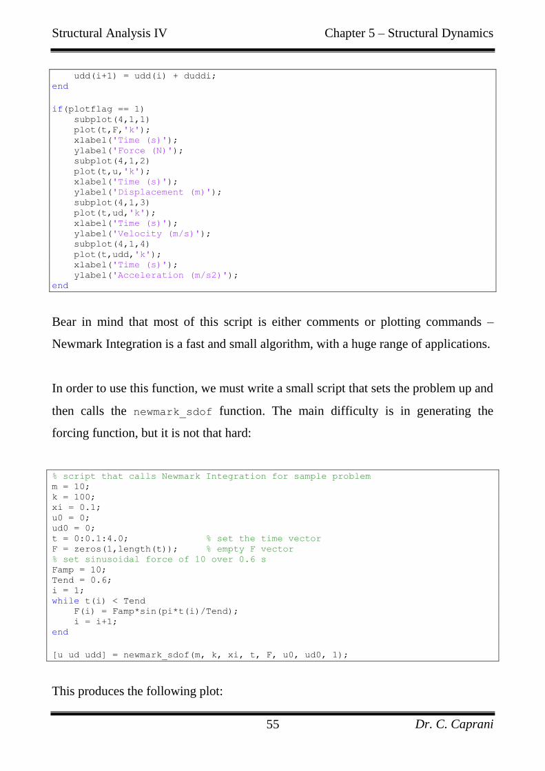
Bear in mind that most of this script is either comments or plotting commands –
Newmark Integration is a fast and small algorithm, with a huge range of applications.
In order to use this function, we must write a small script that sets the problem up and
then calls the newmark_sdof function. The main difficulty is in generating the
forcing function, but it is not that hard:
% script that calls Newmark Integration for sample problem m = 10; k = 100; xi = 0.1; u0 = 0; ud0 = 0; t = 0:0.1:4.0; % set the time vector F = zeros(1,length(t)); % empty F vector % set sinusoidal force of 10 over 0.6 s Famp = 10; Tend = 0.6; i = 1; while t(i) < Tend F(i) = Famp*sin(pi*t(i)/Tend); i = i+1; end
[u ud udd] = newmark_sdof(m, k, xi, t, F, u0, ud0, 1);
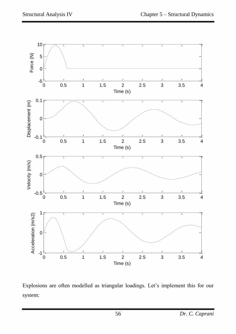
This produces the following plot:
Structural Analysis IV Chapter 5 – Structural Dynamics
Dr. C. Caprani 56
Explosions are often modelled as triangular loadings. Let‟s implement this for our
system:
0 0.5 1 1.5 2 2.5 3 3.5 4-5
0
5
10
Time (s)
Forc
e (
N)
0 0.5 1 1.5 2 2.5 3 3.5 4-0.1
0
0.1
Time (s)
Dis
pla
cem
ent
(m)
0 0.5 1 1.5 2 2.5 3 3.5 4-0.5
0
0.5
Time (s)
Velo
city (
m/s
)
0 0.5 1 1.5 2 2.5 3 3.5 4-1
0
1
Time (s)
Accele
ration (
m/s
2)
Structural Analysis IV Chapter 5 – Structural Dynamics
Dr. C. Caprani 57
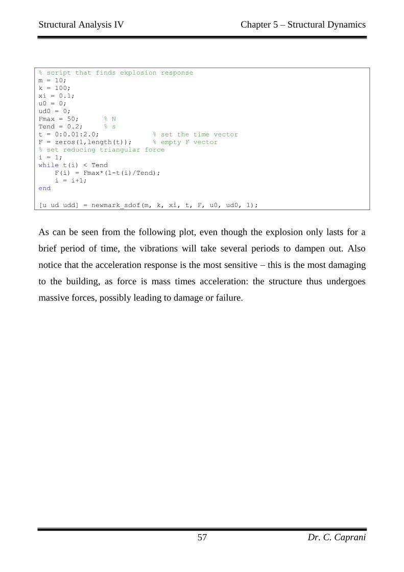
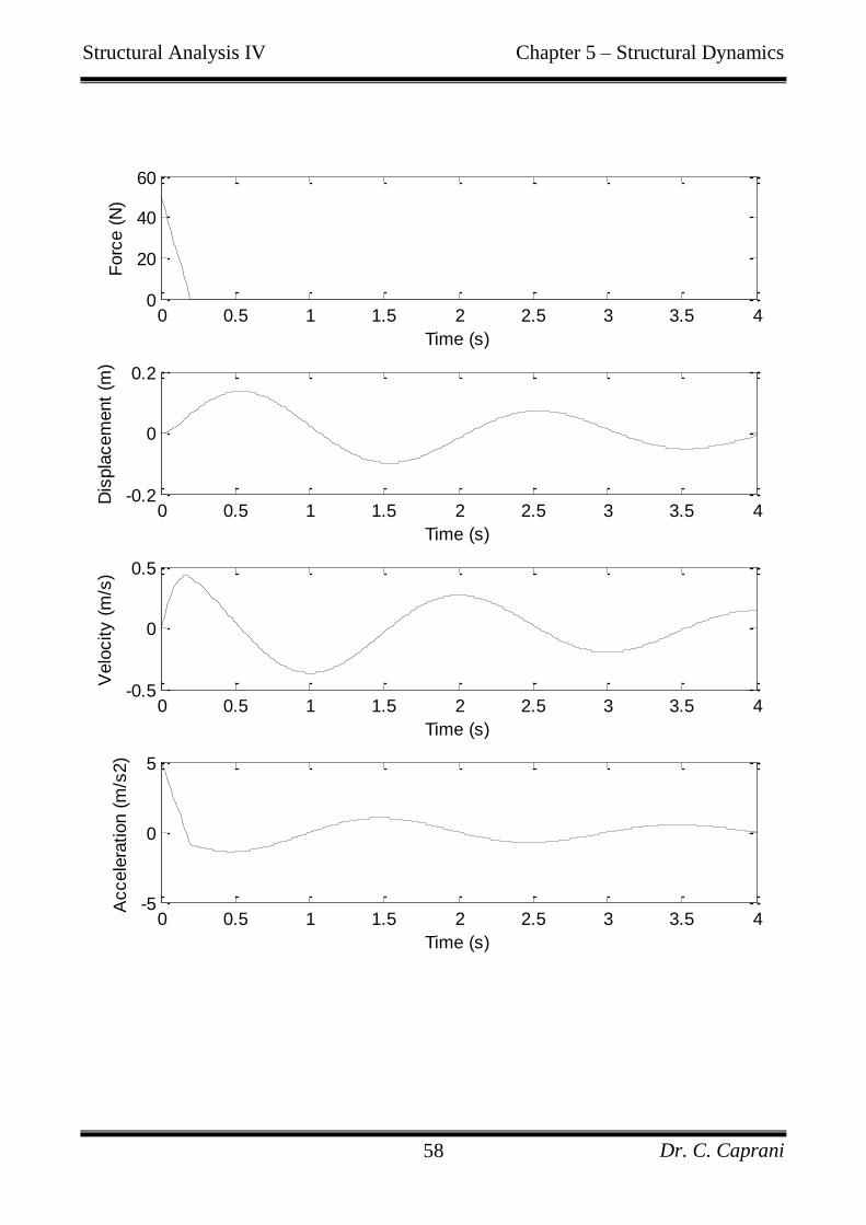
% script that finds explosion response m = 10; k = 100; xi = 0.1; u0 = 0; ud0 = 0; Fmax = 50; % N Tend = 0.2; % s t = 0:0.01:2.0; % set the time vector F = zeros(1,length(t)); % empty F vector % set reducing triangular force i = 1; while t(i) < Tend F(i) = Fmax*(1-t(i)/Tend); i = i+1; end
[u ud udd] = newmark_sdof(m, k, xi, t, F, u0, ud0, 1);
As can be seen from the following plot, even though the explosion only lasts for a
brief period of time, the vibrations will take several periods to dampen out. Also
notice that the acceleration response is the most sensitive – this is the most damaging
to the building, as force is mass times acceleration: the structure thus undergoes
massive forces, possibly leading to damage or failure.
Structural Analysis IV Chapter 5 – Structural Dynamics
Dr. C. Caprani 58
0 0.5 1 1.5 2 2.5 3 3.5 40
20
40
60
Time (s)
Forc
e (
N)
0 0.5 1 1.5 2 2.5 3 3.5 4-0.2
0
0.2
Time (s)
Dis
pla
cem
ent
(m)
0 0.5 1 1.5 2 2.5 3 3.5 4-0.5
0
0.5
Time (s)
Velo
city (
m/s
)
0 0.5 1 1.5 2 2.5 3 3.5 4-5
0
5
Time (s)
Accele
ration (
m/s
2)
Structural Analysis IV Chapter 5 – Structural Dynamics
Dr. C. Caprani 59
5.2.11 Problems
Problem 1
A harmonic oscillation test gave the natural frequency of a water tower to be 0.41 Hz.
Given that the mass of the tank is 150 tonnes, what deflection will result if a 50 kN
horizontal load is applied? You may neglect the mass of the tower.
Ans: 50.2 mm
Problem 2
A 3 m high, 8 m wide single-bay single-storey frame is rigidly jointed with a beam of
mass 5,000 kg and columns of negligible mass and stiffness of EIc = 4.5×10³ kNm
2.
Calculate the natural frequency in lateral vibration and its period. Find the force
required to deflect the frame 25 mm laterally.
Ans: 4.502 Hz; 0.222 sec; 100 kN
Problem 3
An SDOF system (m = 20 kg, k = 350 N/m) is given an initial displacement of 10 mm
and initial velocity of 100 mm/s. (a) Find the natural frequency; (b) the period of
vibration; (c) the amplitude of vibration; and (d) the time at which the third maximum
peak occurs.
Ans: 0.666 Hz; 1.502 sec; 25.91 mm; 3.285 sec.
Problem 4
For the frame of Problem 2, a jack applied a load of 100 kN and then instantaneously
released. On the first return swing a deflection of 19.44 mm was noted. The period of
motion was measured at 0.223 sec. Assuming that the stiffness of the columns cannot
Structural Analysis IV Chapter 5 – Structural Dynamics
Dr. C. Caprani 60
change, find (a) the damping ratio; (b) the coefficient of damping; (c) the undamped
frequency and period; and (d) the amplitude after 5 cycles.
Ans: 0.04; 11,367 kg·s/m; 4.488 Hz; 0.2228 sec; 7.11 mm.
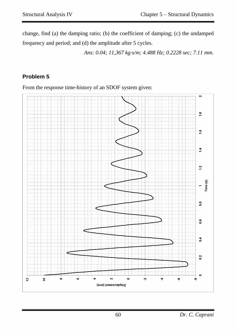
Problem 5
From the response time-history of an SDOF system given:
Structural Analysis IV Chapter 5 – Structural Dynamics
Dr. C. Caprani 61
(a) estimate the damped natural frequency; (b) use the half amplitude method to
calculate the damping ratio; and (c) calculate the undamped natural frequency and
period.
Ans: 4.021 Hz; 0.05; 4.026 Hz; 0.248 sec.
Problem 6
Workers‟ movements on a platform (8 × 6 m high, m = 200 kN) are causing large
dynamic motions. An engineer investigated and found the natural period in sway to
be 0.9 sec. Diagonal remedial ties (E = 200 kN/mm2) are to be installed to reduce the
natural period to 0.3 sec. What tie diameter is required?
Ans: 28.1 mm.
Problem 7
The frame of examples 2.2 and 2.4 has a reciprocating machine put on it. The mass of
this machine is 4 tonnes and is in addition to the mass of the beam. The machine
exerts a periodic force of 8.5 kN at a frequency of 1.75 Hz. (a) What is the steady-
state amplitude of vibration if the damping ratio is 4%? (b) What would the steady-
state amplitude be if the forcing frequency was in resonance with the structure?
Ans: 2.92 mm; 26.56 mm.
Problem 8
An air conditioning unit of mass 1,600 kg is place in the middle (point C) of an 8 m
long simply supported beam (EI = 8×10³ kNm
2) of negligible mass. The motor runs
at 300 rpm and produces an unbalanced load of 120 kg. Assuming a damping ratio of
5%, determine the steady-state amplitude and deflection at C. What rpm will result in
resonance and what is the associated deflection?
Ans: 1.41 mm; 22.34 mm; 206.7 rpm; 36.66 mm.
Structural Analysis IV Chapter 5 – Structural Dynamics
Dr. C. Caprani 62
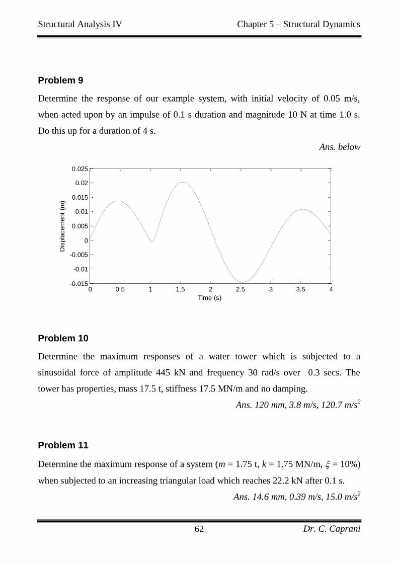
Problem 9
Determine the response of our example system, with initial velocity of 0.05 m/s,
when acted upon by an impulse of 0.1 s duration and magnitude 10 N at time 1.0 s.
Do this up for a duration of 4 s.
Ans. below
Problem 10
Determine the maximum responses of a water tower which is subjected to a
sinusoidal force of amplitude 445 kN and frequency 30 rad/s over 0.3 secs. The
tower has properties, mass 17.5 t, stiffness 17.5 MN/m and no damping.
Ans. 120 mm, 3.8 m/s, 120.7 m/s2
Problem 11
Determine the maximum response of a system (m = 1.75 t, k = 1.75 MN/m, = 10%)
when subjected to an increasing triangular load which reaches 22.2 kN after 0.1 s.
Ans. 14.6 mm, 0.39 m/s, 15.0 m/s2
0 0.5 1 1.5 2 2.5 3 3.5 4-0.015
-0.01
-0.005
0
0.005
0.01
0.015
0.02
0.025
Time (s)
Dis
pla
cem
ent
(m)
Structural Analysis IV Chapter 5 – Structural Dynamics
Dr. C. Caprani 63
5.3 Multi-Degree-of-Freedom Systems
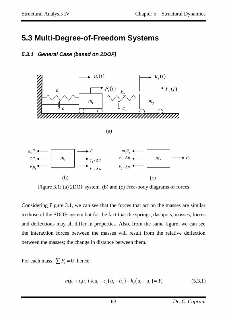
5.3.1 General Case (based on 2DOF)
(a)
(b) (c)
Figure 3.1: (a) 2DOF system. (b) and (c) Free-body diagrams of forces
Considering Figure 3.1, we can see that the forces that act on the masses are similar
to those of the SDOF system but for the fact that the springs, dashpots, masses, forces
and deflections may all differ in properties. Also, from the same figure, we can see
the interaction forces between the masses will result from the relative deflection
between the masses; the change in distance between them.
For each mass, 0x
F , hence:
1 1 1 1 1 1 2 1 2 2 1 2 1mu c u k u c u u k u u F (5.3.1)
Structural Analysis IV Chapter 5 – Structural Dynamics
Dr. C. Caprani 64
2 2 2 2 1 2 2 1 2m u c u u k u u F (5.3.2)
In which we have dropped the time function indicators and allowed u and u to
absorb the directions of the interaction forces. Re-arranging we get:
1 1 1 1 2 2 2 1 1 2 2 2 1
2 2 1 2 2 2 1 2 2 2 2
u m u c c u c u k k u k F
u m u c u c u k u k F
(5.3.3)
This can be written in matrix form:
1 1 1 2 2 1 1 2 2 1 1
2 2 2 2 2 2 2 2 2
0
0
m u c c c u k k k u F
m u c c u k k u F
(5.3.4)
Or another way:
Mu + Cu + Ku = F (5.3.5)
where:
M is the mass matrix (diagonal matrix);
u is the vector of the accelerations for each DOF;
C is the damping matrix (symmetrical matrix);
u is the vector of velocity for each DOF;
K is the stiffness matrix (symmetrical matrix);
u is the vector of displacements for each DOF;
F is the load vector.
Equation (5.3.5) is quite general and reduces to many forms of analysis:
Structural Analysis IV Chapter 5 – Structural Dynamics
Dr. C. Caprani 65
Free vibration:
Mu + Cu + Ku = 0 (5.3.6)
Undamped free vibration:
Mu + Ku = 0 (5.3.7)
Undamped forced vibration:
Mu + Ku = F (5.3.8)
Static analysis:
Ku = F (5.3.9)
We will restrict our attention to the case of undamped free-vibration – equation
(5.3.7) - as the inclusion of damping requires an increase in mathematical complexity
which would distract from our purpose.
Structural Analysis IV Chapter 5 – Structural Dynamics
Dr. C. Caprani 66
5.3.2 Free-Undamped Vibration of 2DOF Systems
The solution to (5.3.7) follows the same methodology as for the SDOF case; so
following that method (equation (2.42)), we propose a solution of the form:
sin t u = a (5.3.10)
where a is the vector of amplitudes corresponding to each degree of freedom. From
this we get:
2 2sin t u = a u (5.3.11)
Then, substitution of (5.3.10) and (5.3.11) into (5.3.7) yields:
2 sin sint t Ma + Ka = 0 (5.3.12)
Since the sine term is constant for each term:
2 K M a = 0 (5.3.13)
We note that in a dynamics problem the amplitudes of each DOF will be non-zero,
hence, a 0 in general. In addition we see that the problem is a standard eigenvalues
problem. Hence, by Cramer‟s rule, in order for (5.3.13) to hold the determinant of
2K M must then be zero:
2 0K M = (5.3.14)
For the 2DOF system, we have:
Structural Analysis IV Chapter 5 – Structural Dynamics
Dr. C. Caprani 67
2 2 2 2
2 1 1 2 2 20k k m k m k K M = (5.3.15)
Expansion of (5.3.15) leads to an equation in 2 called the characteristic polynomial
of the system. The solutions of 2 to this equation are the eigenvalues of 2 K M
. There will be two solutions or roots of the characteristic polynomial in this case and
an n-DOF system has n solutions to its characteristic polynomial. In our case, this
means there are two values of 2 ( 2
1 and 2
2 ) that will satisfy the relationship; thus
there are two frequencies for this system (the lowest will be called the fundamental
frequency). For each 2
n substituted back into (5.3.13), we will get a certain
amplitude vector n
a . This means that each frequency will have its own characteristic
displaced shape of the degrees of freedoms called the mode shape. However, we will
not know the absolute values of the amplitudes as it is a free-vibration problem;
hence we express the mode shapes as a vector of relative amplitudes, nφ , relative to,
normally, the first value in n
a .
As we will see in the following example, the implication of the above is that MDOF
systems vibrate, not just in the fundamental mode, but also in higher harmonics.
From our analysis of SDOF systems it‟s apparent that should any loading coincide
with any of these harmonics, large DAF‟s will result (Section 2.d). Thus, some modes
may be critical design cases depending on the type of harmonic loading as will be
seen later.
Structural Analysis IV Chapter 5 – Structural Dynamics
Dr. C. Caprani 68
5.3.3 Example of a 2DOF System
The two-storey building shown (Figure
3.2) has very stiff floor slabs relative to
the supporting columns. Calculate the
natural frequencies and mode shapes.
3 24.5 10 kNmc
EI
Figure 3.2: Shear frame problem.
Figure 3.3: 2DOF model of the shear frame.
We will consider the free lateral vibrations of the two-storey shear frame idealised as
in Figure 3.3. The lateral, or shear stiffness of the columns is:
1 2 3
6
3
6
122
2 12 4.5 10
3
4 10 N/m
cEI
k k kh
k
The characteristic polynomial is as given in (5.3.15) so we have:
Structural Analysis IV Chapter 5 – Structural Dynamics
Dr. C. Caprani 69
6 2 6 2 12
6 4 10 2 12
8 10 5000 4 10 3000 16 10 0
15 10 4.4 10 16 10 0
This is a quadratic equation in 2 and so can be solved using 615 10a ,
104.4 10b and 1216 10c in the usual expression
2
2 4
2
b b ac
a
Hence we get 2
1425.3 and 2
22508 . This may be written:
2425.3
2508n
ω hence 20.6
50.1n
ω rad/s and 3.28
7.972
n
ωf Hz
To solve for the mode shapes, we will use the appropriate form of the equation of
motion, equation (5.3.13): 2 K M a = 0 . First solve for the
2 E K M
matrix and then solve Ea = 0 for the amplitudes n
a . Then, form nφ .
In general, for a 2DOF system, we have:
2
1 2 2 1 1 2 1 22
2
2 2 2 2 2 2
0
0
n
n n
n
k k k m k k m k
k k m k k m
E
For 2
1425.3 :
6
1
5.8735 410
4 2.7241
E
Structural Analysis IV Chapter 5 – Structural Dynamics
Dr. C. Caprani 70
Hence
16
1 1
2
5.8735 4 010
4 2.7241 0
a
a
E a
Taking either equation, we calculate:
1 2 1 2
1 1
1 2 1 2
5.8735 4 0 0.681 1
4 2.7241 0 0.681 0.681
a a a a
a a a a
φ
Similarly for 2
22508 :
6
2
4.54 410
4 3.524
E
Hence, again taking either equation, we calculate:
1 2 1 2
2 1
1 2 1 2
4.54 4 0 0.881 1
4 3.524 0 0.881 0.881
a a a a
a a a a
φ
The complete solution may be given by the following two matrices which are used in
further analysis for more complicated systems.
2425.3
2508n
ω and 1 1
1.468 1.135
Φ
For our frame, we can sketch these two frequencies and associated mode shapes:
Figure 3.4.
Structural Analysis IV Chapter 5 – Structural Dynamics
Dr. C. Caprani 71
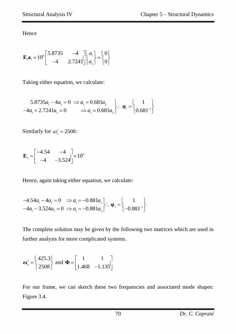
Figure 3.4: Mode shapes and frequencies of the example frame.
Larger and more complex structures will have many degrees of freedom and hence
many natural frequencies and mode shapes. There are different mode shapes for
different forms of deformation; torsional, lateral and vertical for example. Periodic
loads acting in these directions need to be checked against the fundamental frequency
for the type of deformation; higher harmonics may also be important.
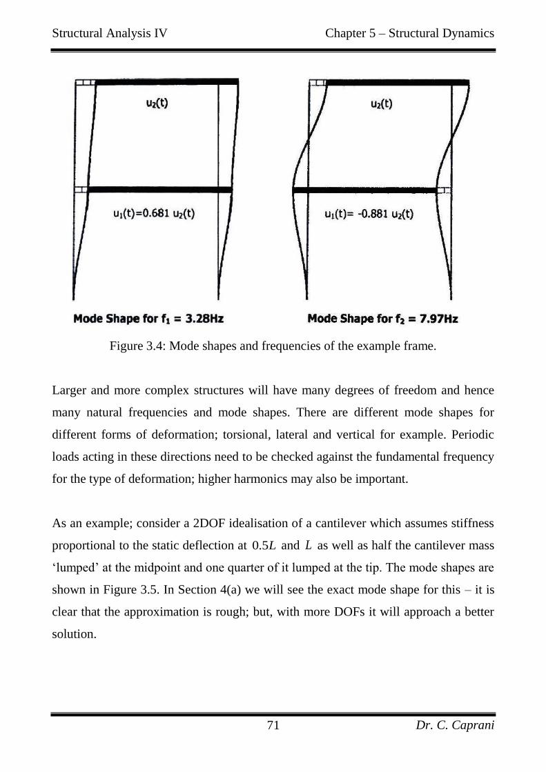
As an example; consider a 2DOF idealisation of a cantilever which assumes stiffness
proportional to the static deflection at 0.5L and L as well as half the cantilever mass
„lumped‟ at the midpoint and one quarter of it lumped at the tip. The mode shapes are
shown in Figure 3.5. In Section 4(a) we will see the exact mode shape for this – it is
clear that the approximation is rough; but, with more DOFs it will approach a better
solution.
Structural Analysis IV Chapter 5 – Structural Dynamics
Dr. C. Caprani 72
Figure 3.5: Lumped mass, 2DOF idealisation of a cantilever.
Mode 1
Mode 2
Structural Analysis IV Chapter 5 – Structural Dynamics
Dr. C. Caprani 73
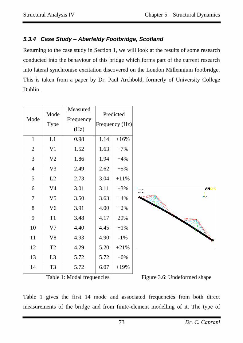
5.3.4 Case Study – Aberfeldy Footbridge, Scotland
Returning to the case study in Section 1, we will look at the results of some research
conducted into the behaviour of this bridge which forms part of the current research
into lateral synchronise excitation discovered on the London Millennium footbridge.
This is taken from a paper by Dr. Paul Archbold, formerly of University College
Dublin.
Mode Mode
Type
Measured
Frequency
(Hz)
Predicted
Frequency (Hz)
1 L1 0.98 1.14 +16%
2 V1 1.52 1.63 +7%
3 V2 1.86 1.94 +4%
4 V3 2.49 2.62 +5%
5 L2 2.73 3.04 +11%
6 V4 3.01 3.11 +3%
7 V5 3.50 3.63 +4%
8 V6 3.91 4.00 +2%
9 T1 3.48 4.17 20%
10 V7 4.40 4.45 +1%
11 V8 4.93 4.90 -1%
12 T2 4.29 5.20 +21%
13 L3 5.72 5.72 +0%
14 T3 5.72 6.07 +19%
Table 1: Modal frequencies Figure 3.6: Undeformed shape
Table 1 gives the first 14 mode and associated frequencies from both direct
measurements of the bridge and from finite-element modelling of it. The type of
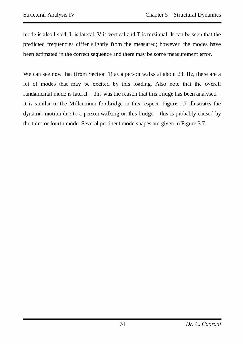
Structural Analysis IV Chapter 5 – Structural Dynamics
Dr. C. Caprani 74
mode is also listed; L is lateral, V is vertical and T is torsional. It can be seen that the
predicted frequencies differ slightly from the measured; however, the modes have
been estimated in the correct sequence and there may be some measurement error.
We can see now that (from Section 1) as a person walks at about 2.8 Hz, there are a
lot of modes that may be excited by this loading. Also note that the overall
fundamental mode is lateral – this was the reason that this bridge has been analysed –
it is similar to the Millennium footbridge in this respect. Figure 1.7 illustrates the
dynamic motion due to a person walking on this bridge – this is probably caused by
the third or fourth mode. Several pertinent mode shapes are given in Figure 3.7.
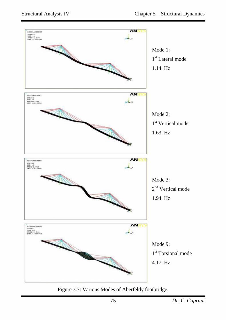
Structural Analysis IV Chapter 5 – Structural Dynamics
Dr. C. Caprani 75
Mode 1:
1st Lateral mode
1.14 Hz
Mode 2:
1st Vertical mode
1.63 Hz
Mode 3:
2nd
Vertical mode
1.94 Hz
Mode 9:
1st Torsional mode
4.17 Hz
Figure 3.7: Various Modes of Aberfeldy footbridge.
Structural Analysis IV Chapter 5 – Structural Dynamics
Dr. C. Caprani 76
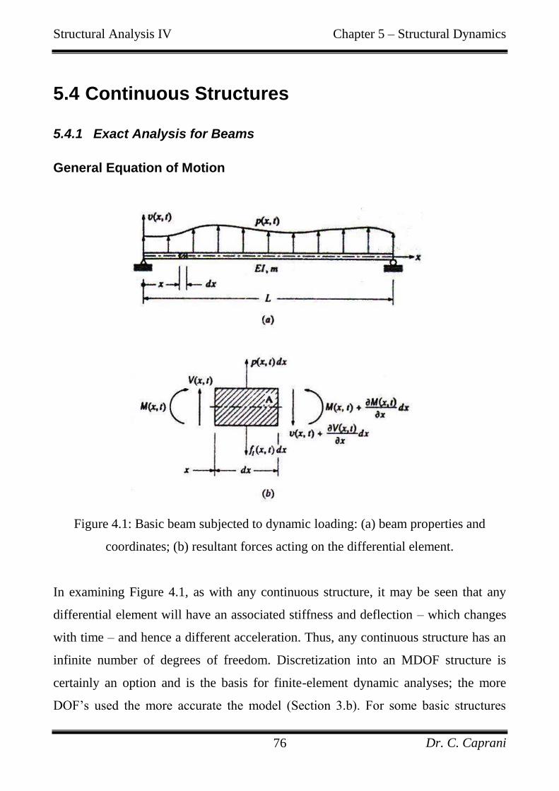
5.4 Continuous Structures
5.4.1 Exact Analysis for Beams
General Equation of Motion
Figure 4.1: Basic beam subjected to dynamic loading: (a) beam properties and
coordinates; (b) resultant forces acting on the differential element.
In examining Figure 4.1, as with any continuous structure, it may be seen that any
differential element will have an associated stiffness and deflection – which changes
with time – and hence a different acceleration. Thus, any continuous structure has an
infinite number of degrees of freedom. Discretization into an MDOF structure is
certainly an option and is the basis for finite-element dynamic analyses; the more
DOF‟s used the more accurate the model (Section 3.b). For some basic structures
Structural Analysis IV Chapter 5 – Structural Dynamics
Dr. C. Caprani 77
though, the exact behaviour can be explicitly calculated. We will limit ourselves to
free-undamped vibration of beams that are thin in comparison to their length. A
general expression can be derived and from this, several usual cases may be
established.
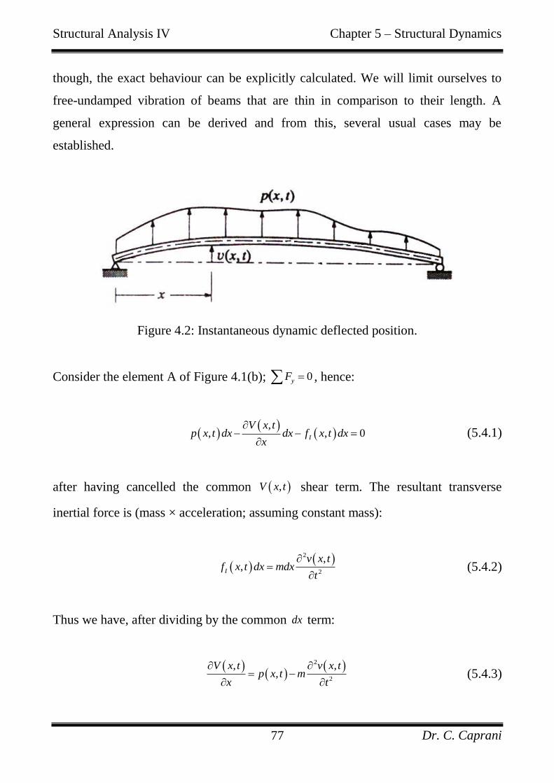
Figure 4.2: Instantaneous dynamic deflected position.
Consider the element A of Figure 4.1(b); , hence:
(5.4.1)
after having cancelled the common shear term. The resultant transverse
inertial force is (mass × acceleration; assuming constant mass):
(5.4.2)
Thus we have, after dividing by the common term:
(5.4.3)
0yF
,
, , 0I
V x tp x t dx dx f x t dx
x
,V x t
2
2
,,I
v x tf x t dx mdx
t
dx
2
2
, ,,
V x t v x tp x t m
x t

Structural Analysis IV Chapter 5 – Structural Dynamics
Dr. C. Caprani 78
which, with no acceleration, is the usual static relationship between shear force and
applied load. By taking moments about the point A on the element, and dropping
second order and common terms, we get the usual expression:
(5.4.4)
Differentiating this with respect to and substituting into (5.4.3), in addition to the
relationship (which assumes that the beam is of constant stiffness):
(5.4.5)
With free vibration this is:
(5.4.6)
,
,M x t
V x tx
x
2
2vM EI
x
4 2
4 2
, ,,
v x t v x tEI m p x t
x t
4 2
4 2
, ,0
v x t v x tEI m
x t
Structural Analysis IV Chapter 5 – Structural Dynamics
Dr. C. Caprani 79
General Solution for Free-Undamped Vibration
Examination of equation (5.4.6) yields several aspects:
It is separated into spatial ( ) and temporal ( ) terms and we may assume that the
solution is also;
It is a fourth-order differential in ; hence we will need four spatial boundary
conditions to solve – these will come from the support conditions at each end;
It is a second order differential in and so we will need two temporal initial
conditions to solve – initial deflection and velocity at a point for example.
To begin, assume the solution is of a form of separated variables:
(5.4.7)
where will define the deformed shape of the beam and the amplitude of
vibration. Inserting the assumed solution into (5.4.6) and collecting terms we have:
(5.4.8)
This follows as the terms each side of the equals are functions of and separately
and so must be constant. Hence, each function type (spatial or temporal) is equal to
and so we have:
(5.4.9)
(5.4.10)
x t
x
t
,v x t x Y t
x Y t
4 2
2
4 2
1 1constant
x Y tEI
m x x Y t t
x t
2
4
2
4
xEI m x
x
2 0Y t Y t
Structural Analysis IV Chapter 5 – Structural Dynamics
Dr. C. Caprani 80
Equation (5.4.10) is the same as for an SDOF system (equation (2.4)) and so the
solution must be of the same form (equation (2.17)):
(5.4.11)
In order to evaluate we will use equation (5.4.9) and we introduce:
2
4 m
EI
(5.4.12)
And assuming a solution of the form , substitution into (5.4.9) gives:
4 4 exp 0s G sx (5.4.13)
There are then four roots for and when each is put into (5.4.13) and added we get:
1 2 3 4exp exp exp expx G i x G i x G x G x (5.4.14)
In which the ‟s may be complex constant numbers, but, by using Euler‟s
expressions for cos, sin, sinh and cosh we get:
1 2 3 4sin cos sinh coshx A x A x A x A x (5.4.15)
where the ‟s are now real constants; three of which may be evaluated through the
boundary conditions; the fourth however is arbitrary and will depend on .
00 cos sin
YY t Y t t
exp( )x G sx
s
G
A
Structural Analysis IV Chapter 5 – Structural Dynamics
Dr. C. Caprani 81
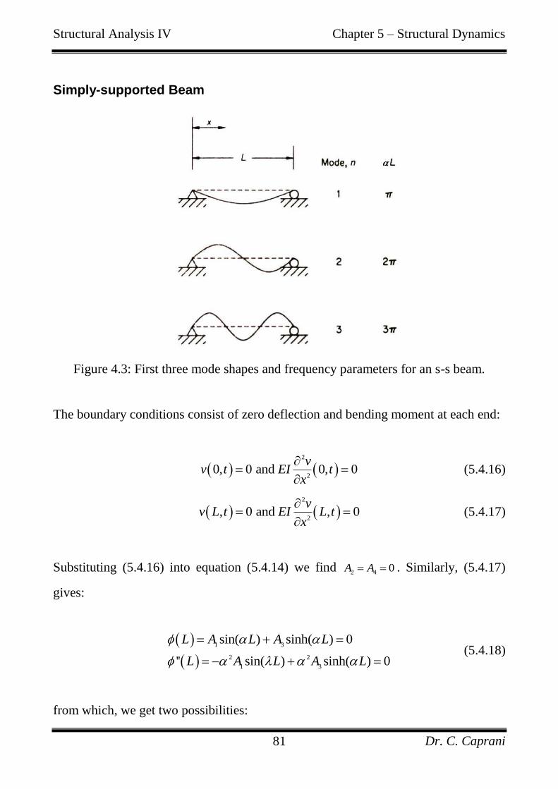
Simply-supported Beam
Figure 4.3: First three mode shapes and frequency parameters for an s-s beam.
The boundary conditions consist of zero deflection and bending moment at each end:
2
20, 0 and 0, 0
vv t EI t
x
(5.4.16)
2
2, 0 and , 0
vv L t EI L t
x
(5.4.17)
Substituting (5.4.16) into equation (5.4.14) we find . Similarly, (5.4.17)
gives:
1 3
2 2
1 3
sin( ) sinh( ) 0
'' sin( ) sinh( ) 0
L A L A L
L A L A L
(5.4.18)
from which, we get two possibilities:
2 4 0A A
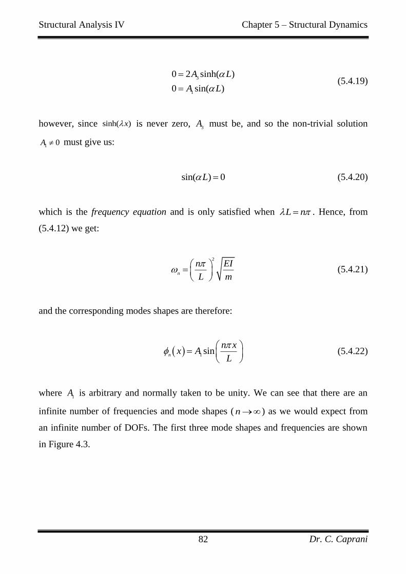
Structural Analysis IV Chapter 5 – Structural Dynamics
Dr. C. Caprani 82
3
1
0 2 sinh( )
0 sin( )
A L
A L
(5.4.19)
however, since is never zero, 3
A must be, and so the non-trivial solution
must give us:
sin( ) 0L (5.4.20)
which is the frequency equation and is only satisfied when L n . Hence, from
(5.4.12) we get:
2
n
n EI
L m
(5.4.21)
and the corresponding modes shapes are therefore:
1sin
n
n xx A
L
(5.4.22)
where 1
A is arbitrary and normally taken to be unity. We can see that there are an
infinite number of frequencies and mode shapes ( n) as we would expect from
an infinite number of DOFs. The first three mode shapes and frequencies are shown
in Figure 4.3.
sinh( )x
1 0A
Structural Analysis IV Chapter 5 – Structural Dynamics
Dr. C. Caprani 83
Cantilever Beam
This example is important as it describes the sway behaviour of tall buildings. The
boundary conditions consist of:
0, 0 and 0, 0v
v t tx
(5.4.23)
2 3
2 3, 0 and , 0
v vEI L t EI L t
x x
(5.4.24)
Which represent zero displacement and slope at the support and zero bending
moment and shear at the tip. Substituting (5.4.23) into equation (5.4.14) we get
4 2A A and
3 1A A . Similarly, (5.4.24) gives:
2 2 2 2
1 2 3 4
3 3 3 3
1 2 3 4
'' sin( ) cos( ) sinh( ) cosh( ) 0
''' cos( ) sin( ) cosh( ) sinh( ) 0
L A L A L A L A L
L A L A L A L A L
(5.4.25)
where a prime indicates a derivate of x , and so we find:
1 2
1 2
sin( ) sinh( ) cos( ) cosh( ) 0
cos( ) cosh( ) sin( ) sinh( ) 0
A L L A L L
A L L A L L
(5.4.26)
Solving for 1
A and 2
A we find:
2
1
2
2
cos( ) cosh( )0
sin( ) sinh( ) sin( ) sinh( )
cos( ) cosh( )0
sin( ) sinh( ) sin( ) sinh( )
L LA
L L L L
L LA
L L L L
(5.4.27)
Structural Analysis IV Chapter 5 – Structural Dynamics
Dr. C. Caprani 84
In order that neither 1
A and 2
A are zero, the expression in the brackets must be zero
and we are left with the frequency equation:
cos( )cosh( ) 1 0L L (5.4.28)
The mode shape is got by expressing 2
A in terms of 1
A :
2 1
sin( ) sinh( )
cos( ) cosh( )
L LA A
L L
(5.4.29)
and the modes shapes are therefore:
1
sin( ) sinh( )
sin( ) sinh( )cosh( ) cos( )
cos( ) cosh( )
n
x x
x A L Lx x
L L
(5.4.30)
where again1
A is arbitrary and normally taken to be unity. We can see from (5.4.28)
that it must be solved numerically for the corresponding values of L The natural
frequencies are then got from (5.4.21) with the substitution of L for n . The first
three mode shapes and frequencies are shown in Figure 4.4.
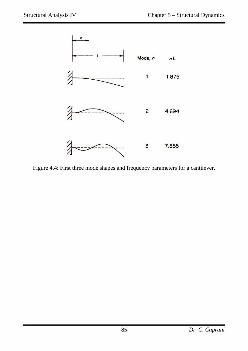
Structural Analysis IV Chapter 5 – Structural Dynamics
Dr. C. Caprani 85
Figure 4.4: First three mode shapes and frequency parameters for a cantilever.
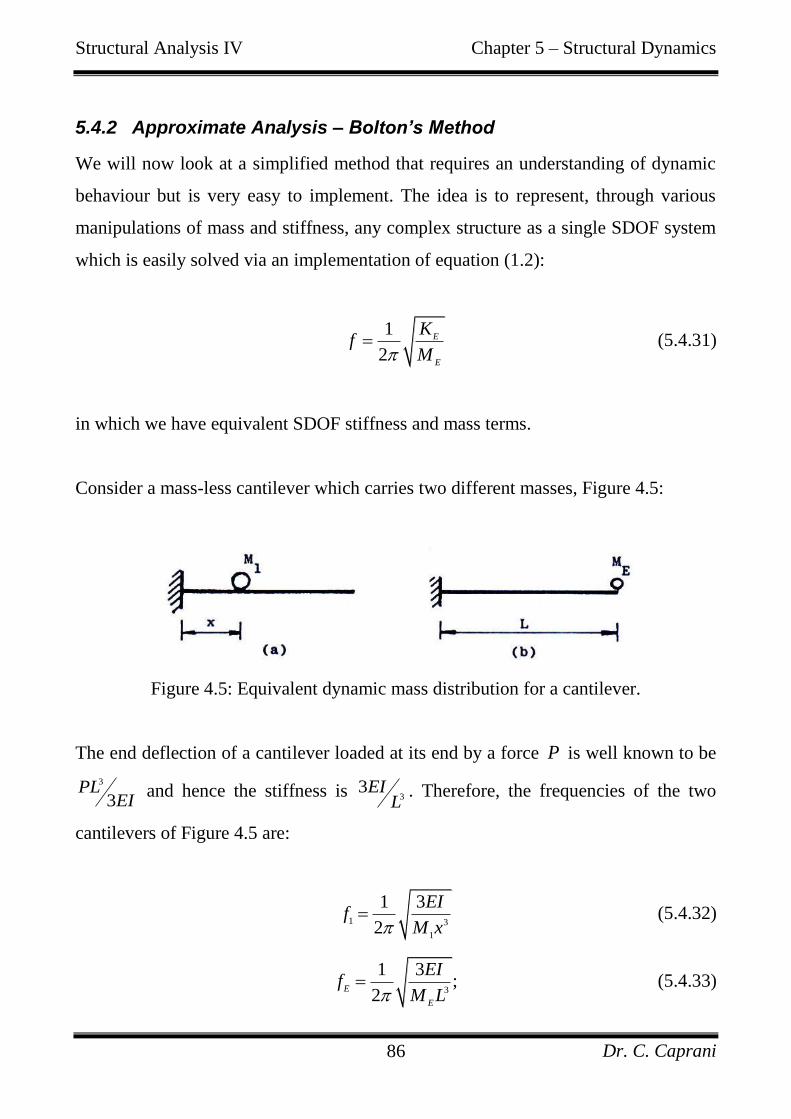
Structural Analysis IV Chapter 5 – Structural Dynamics
Dr. C. Caprani 86
5.4.2 Approximate Analysis – Bolton’s Method
We will now look at a simplified method that requires an understanding of dynamic
behaviour but is very easy to implement. The idea is to represent, through various
manipulations of mass and stiffness, any complex structure as a single SDOF system
which is easily solved via an implementation of equation (1.2):
1
2
E
E
Kf
M (5.4.31)
in which we have equivalent SDOF stiffness and mass terms.
Consider a mass-less cantilever which carries two different masses, Figure 4.5:
Figure 4.5: Equivalent dynamic mass distribution for a cantilever.
The end deflection of a cantilever loaded at its end by a force P is well known to be
3
3PL
EI and hence the stiffness is 3
3EIL
. Therefore, the frequencies of the two
cantilevers of Figure 4.5 are:
1 3
1
1 3
2
EIf
M x (5.4.32)
3
1 3;
2E
E
EIf
M L (5.4.33)
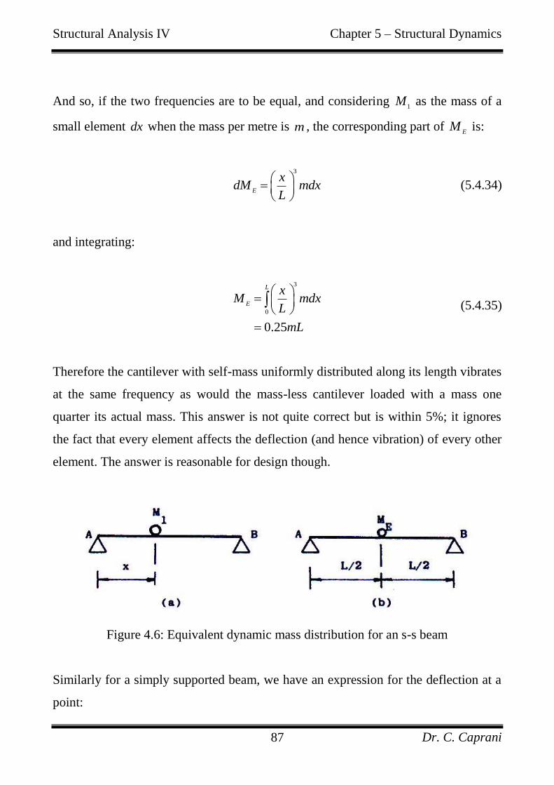
Structural Analysis IV Chapter 5 – Structural Dynamics
Dr. C. Caprani 87
And so, if the two frequencies are to be equal, and considering 1
M as the mass of a
small element dx when the mass per metre is m , the corresponding part of E
M is:
3
E
xdM mdx
L
(5.4.34)
and integrating:
3
0
0.25
L
E
xM mdx
L
mL
(5.4.35)
Therefore the cantilever with self-mass uniformly distributed along its length vibrates
at the same frequency as would the mass-less cantilever loaded with a mass one
quarter its actual mass. This answer is not quite correct but is within 5%; it ignores
the fact that every element affects the deflection (and hence vibration) of every other
element. The answer is reasonable for design though.
Figure 4.6: Equivalent dynamic mass distribution for an s-s beam
Similarly for a simply supported beam, we have an expression for the deflection at a
point:
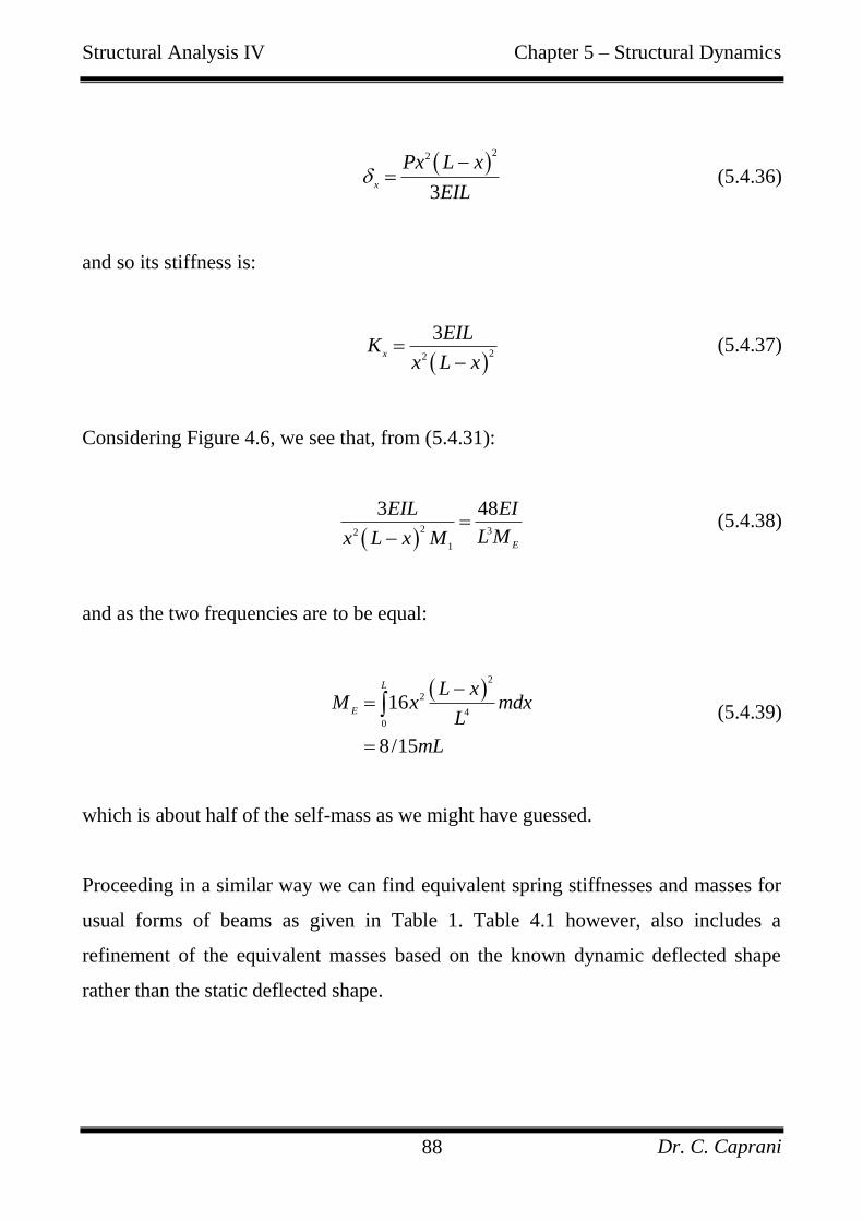
Structural Analysis IV Chapter 5 – Structural Dynamics
Dr. C. Caprani 88
22
3x
Px L x
EIL
(5.4.36)
and so its stiffness is:
22
3x
EILK
x L x
(5.4.37)
Considering Figure 4.6, we see that, from (5.4.31):
2 32
1
3 48
E
EIL EI
L Mx L x M
(5.4.38)
and as the two frequencies are to be equal:
2
2
40
16
8/15
L
E
L xM x mdx
L
mL
(5.4.39)
which is about half of the self-mass as we might have guessed.
Proceeding in a similar way we can find equivalent spring stiffnesses and masses for
usual forms of beams as given in Table 1. Table 4.1 however, also includes a
refinement of the equivalent masses based on the known dynamic deflected shape
rather than the static deflected shape.
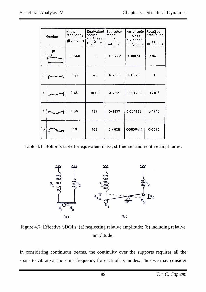
Structural Analysis IV Chapter 5 – Structural Dynamics
Dr. C. Caprani 89
Table 4.1: Bolton‟s table for equivalent mass, stiffnesses and relative amplitudes.
Figure 4.7: Effective SDOFs: (a) neglecting relative amplitude; (b) including relative
amplitude.
In considering continuous beams, the continuity over the supports requires all the
spans to vibrate at the same frequency for each of its modes. Thus we may consider
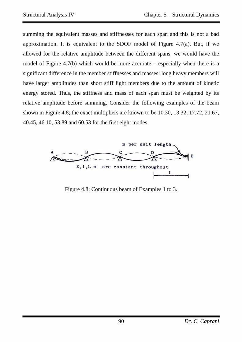
Structural Analysis IV Chapter 5 – Structural Dynamics
Dr. C. Caprani 90
summing the equivalent masses and stiffnesses for each span and this is not a bad
approximation. It is equivalent to the SDOF model of Figure 4.7(a). But, if we
allowed for the relative amplitude between the different spans, we would have the
model of Figure 4.7(b) which would be more accurate – especially when there is a
significant difference in the member stiffnesses and masses: long heavy members will
have larger amplitudes than short stiff light members due to the amount of kinetic
energy stored. Thus, the stiffness and mass of each span must be weighted by its
relative amplitude before summing. Consider the following examples of the beam
shown in Figure 4.8; the exact multipliers are known to be 10.30, 13.32, 17.72, 21.67,
40.45, 46.10, 53.89 and 60.53 for the first eight modes.
Figure 4.8: Continuous beam of Examples 1 to 3.
Structural Analysis IV Chapter 5 – Structural Dynamics
Dr. C. Caprani 91
Example 1: Ignoring relative amplitude and refined ME
From Table 4.1, and the previous discussion:
3
48 3 101.9E
EIK
L ; and
8 13
15 2E
M mL
,
and applying (5.4.31) we have: 4
110.82
2
EIf
mL
The multiplier in the exact answer is 10.30: an error of 5%.
Example 2: Including relative amplitude and refined ME
From Table 4.1 and the previous discussion, we have:
3 3 3
48 101.93 1 0.4108 185.9
E
EI EI EIK
L L L
3 0.4928 1 0.4299 0.4108 1.655E
M mL mL mL
and applying (5.4.31) we have:
4
110.60
2
EIf
mL
The multiplier in the exact answer is 10.30: a reduced error of 2.9%.
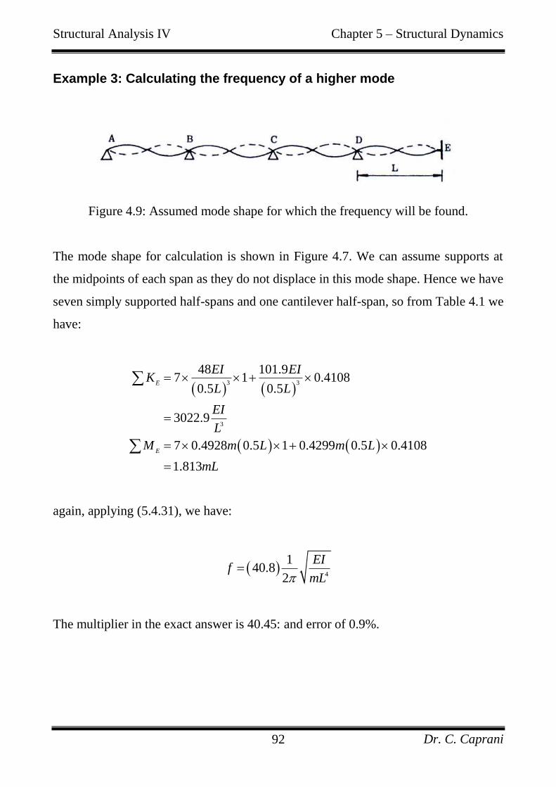
Structural Analysis IV Chapter 5 – Structural Dynamics
Dr. C. Caprani 92
Example 3: Calculating the frequency of a higher mode
Figure 4.9: Assumed mode shape for which the frequency will be found.
The mode shape for calculation is shown in Figure 4.7. We can assume supports at
the midpoints of each span as they do not displace in this mode shape. Hence we have
seven simply supported half-spans and one cantilever half-span, so from Table 4.1 we
have:
3 3
3
48 101.97 1 0.4108
0.5 0.5
3022.9
7 0.4928 0.5 1 0.4299 0.5 0.4108
1.813
E
E
EI EIK
L L
EI
L
M m L m L
mL
again, applying (5.4.31), we have:
4
140.8
2
EIf
mL
The multiplier in the exact answer is 40.45: and error of 0.9%.
Structural Analysis IV Chapter 5 – Structural Dynamics
Dr. C. Caprani 93
Mode Shapes and Frequencies
Section 2.d described how the DAF is very large when a force is applied at the
natural frequency of the structure; so for any structure we can say that when it is
vibrating at its natural frequency it has very low stiffness – and in the case of no
damping: zero stiffness. Higher modes will have higher stiffnesses but stiffness may
also be recognised in one form as
1M
EI R (5.4.40)
where R is the radius of curvature and M is bending moment. Therefore, smaller
stiffnesses have a larger R and larger stiffnesses have a smaller R . Similarly then,
lower modes have a larger R and higher modes have a smaller R . This enables us to
distinguish between modes by their frequencies. Noting that a member in single
curvature (i.e. no point of contraflexure) has a larger R than a member in double
curvature (1 point of contraflexure) which in turn has a larger R than a member in
triple curvature (2 points of contraflexure), we can distinguish modes by deflected
shapes. Figures 4.3 and 4.4 illustrate this clearly.
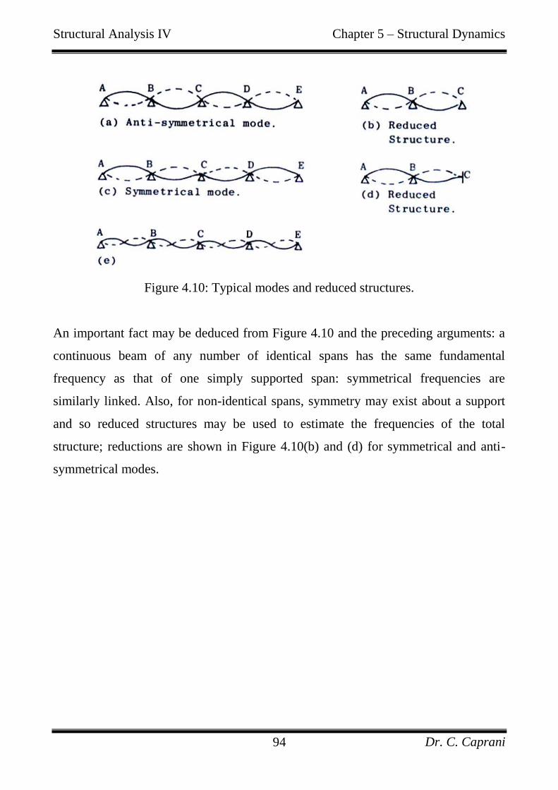
Structural Analysis IV Chapter 5 – Structural Dynamics
Dr. C. Caprani 94
Figure 4.10: Typical modes and reduced structures.
An important fact may be deduced from Figure 4.10 and the preceding arguments: a
continuous beam of any number of identical spans has the same fundamental
frequency as that of one simply supported span: symmetrical frequencies are
similarly linked. Also, for non-identical spans, symmetry may exist about a support
and so reduced structures may be used to estimate the frequencies of the total
structure; reductions are shown in Figure 4.10(b) and (d) for symmetrical and anti-
symmetrical modes.
Structural Analysis IV Chapter 5 – Structural Dynamics
Dr. C. Caprani 95
5.4.3 Problems
Problem 1
Calculate the first natural frequency of a simply supported bridge of mass 7 tonnes
with a 3 tonne lorry at its quarter point. It is known that a load of 10 kN causes a 3
mm deflection.
Ans.: 3.95Hz.
Problem 2
Calculate the first natural frequency of a 4 m long cantilever (EI = 4,320 kNm2)
which carries a mass of 500 kg at its centre and has self weight of 1200 kg.
Ans.: 3.76 Hz.
Problem 3
What is the fundamental frequency of a 3-span continuous beam of spans 4, 8 and 5
m with constant EI and m? What is the frequency when EI = 6×10³ kNm
2 and m =
150 kg/m?
Ans.: 6.74 Hz.
Problem 4
Calculate the first and second natural frequencies of a two-span continuous beam;
fixed at A and on rollers at B and C. Span AB is 8 m with flexural stiffness of 2EI and
a mass of 1.5m. Span BC is 6 m with flexural stiffness EI and mass m per metre.
What are the frequencies when EI = 4.5×10³ kNm
2 and m = 100 kg/m?
Ans.: 9.3 Hz; ? Hz.
Structural Analysis IV Chapter 5 – Structural Dynamics
Dr. C. Caprani 96
Problem 5
Calculate the first and second natural frequencies of a 4-span continuous beam of
spans 4, 5, 4 and 5 m with constant EI and m? What are the frequencies when EI =
4×10³ kNm
2 and m = 120 kg/m? What are the new frequencies when support A is
fixed? Does this make it more or less susceptible to human-induced vibration?
Ans.: ? Hz; ? Hz.
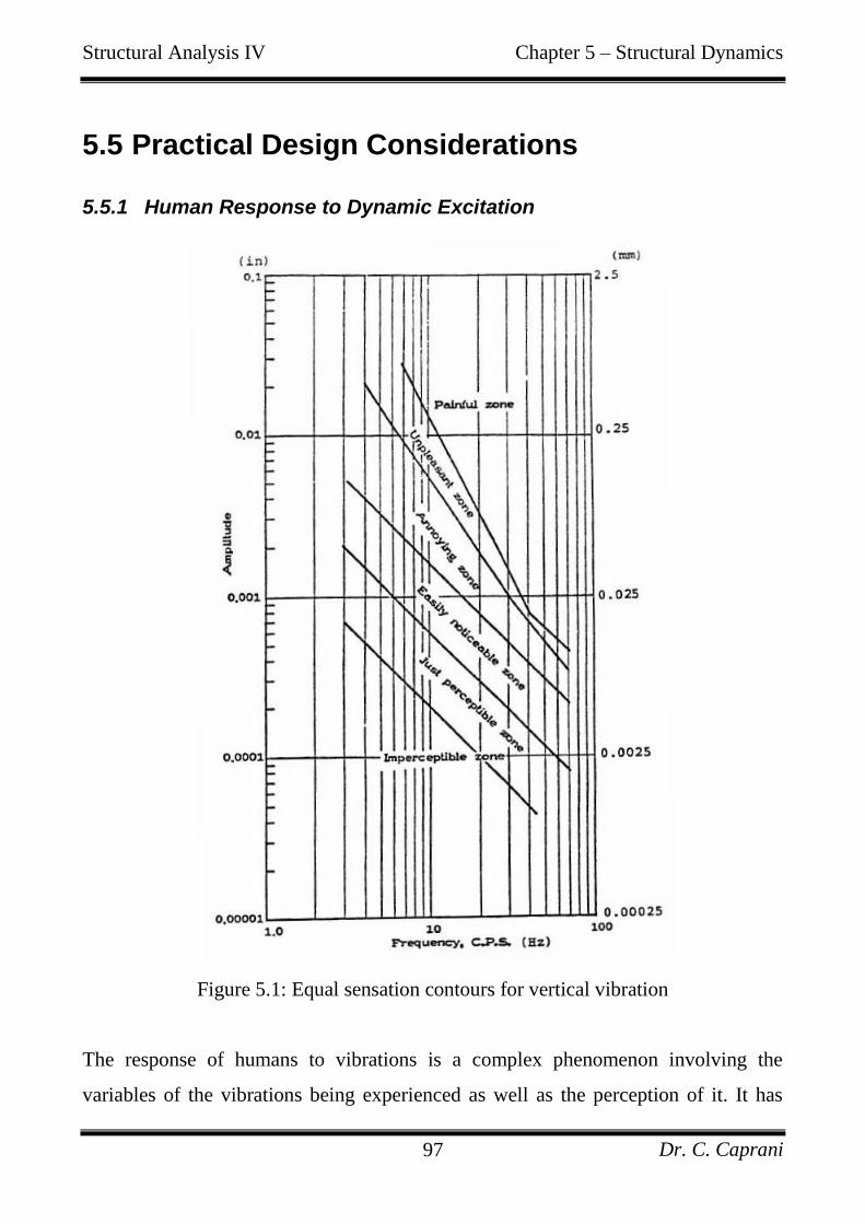
Structural Analysis IV Chapter 5 – Structural Dynamics
Dr. C. Caprani 97
5.5 Practical Design Considerations
5.5.1 Human Response to Dynamic Excitation
Figure 5.1: Equal sensation contours for vertical vibration
The response of humans to vibrations is a complex phenomenon involving the
variables of the vibrations being experienced as well as the perception of it. It has
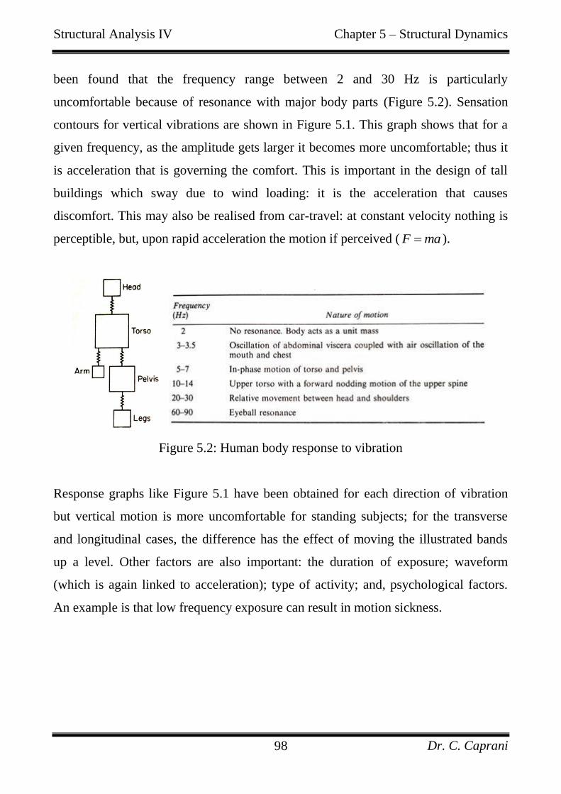
Structural Analysis IV Chapter 5 – Structural Dynamics
Dr. C. Caprani 98
been found that the frequency range between 2 and 30 Hz is particularly
uncomfortable because of resonance with major body parts (Figure 5.2). Sensation
contours for vertical vibrations are shown in Figure 5.1. This graph shows that for a
given frequency, as the amplitude gets larger it becomes more uncomfortable; thus it
is acceleration that is governing the comfort. This is important in the design of tall
buildings which sway due to wind loading: it is the acceleration that causes
discomfort. This may also be realised from car-travel: at constant velocity nothing is
perceptible, but, upon rapid acceleration the motion if perceived ( F ma ).
Figure 5.2: Human body response to vibration
Response graphs like Figure 5.1 have been obtained for each direction of vibration
but vertical motion is more uncomfortable for standing subjects; for the transverse
and longitudinal cases, the difference has the effect of moving the illustrated bands
up a level. Other factors are also important: the duration of exposure; waveform
(which is again linked to acceleration); type of activity; and, psychological factors.
An example is that low frequency exposure can result in motion sickness.
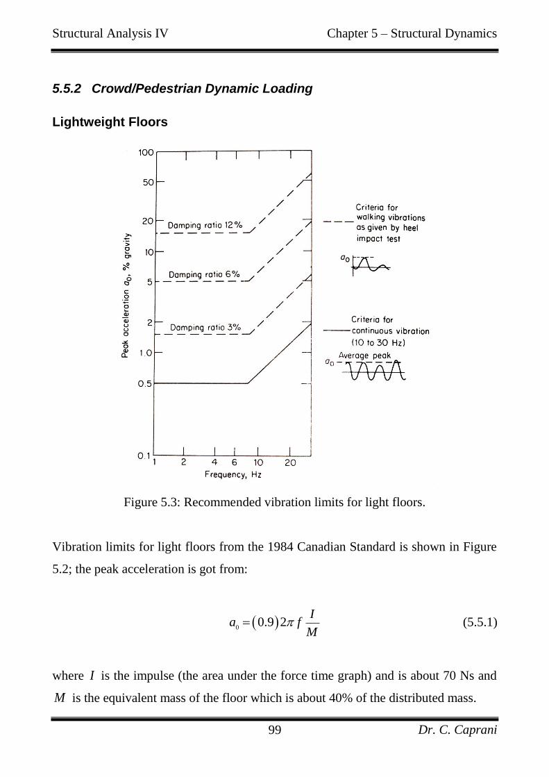
Structural Analysis IV Chapter 5 – Structural Dynamics
Dr. C. Caprani 99
5.5.2 Crowd/Pedestrian Dynamic Loading
Lightweight Floors
Figure 5.3: Recommended vibration limits for light floors.
Vibration limits for light floors from the 1984 Canadian Standard is shown in Figure
5.2; the peak acceleration is got from:
00.9 2
Ia f
M (5.5.1)
where I is the impulse (the area under the force time graph) and is about 70 Ns and
M is the equivalent mass of the floor which is about 40% of the distributed mass.
Structural Analysis IV Chapter 5 – Structural Dynamics
Dr. C. Caprani 100
This form of approach is to be complemented by a simple analysis of an equivalent
SDOF system. Also, as seen in Section 1, by keeping the fundamental frequency
above 5 Hz, human loading should not be problematic.
Structural Analysis IV Chapter 5 – Structural Dynamics
Dr. C. Caprani 101
Crowd Loading
This form of loading occurs in grandstands and similar structures where a large
number of people are densely packed and will be responding to the same stimulus.
Coordinated jumping to the beat of music, for example, can cause a DAF of about
1.97 at about 2.5 Hz. Dancing, however, normally generates frequencies of 2 – 3 Hz.
Once again, by keeping the natural frequency of the structure above about 5 Hz no
undue dynamic effects should be noticed.
In the transverse or longitudinal directions, allowance should also be made due to the
crowd-sway that may accompany some events a value of about 0.3 kN per metre of
seating parallel and 0.15 kN perpendicular to the seating is an approximate method
for design.
Staircases can be subject to considerable dynamic forces as running up or down such
may cause peak loads of up to 4-5 times the persons bodyweight over a period of
about 0.3 seconds – the method for lightweight floors can be applied to this scenario.
Structural Analysis IV Chapter 5 – Structural Dynamics
Dr. C. Caprani 102
Footbridges
As may be gathered from the Case Studies of the Aberfeldy Bridge, the problem is
complex, however some rough guidelines are possible. Once again controlling the
fundamental frequency is important; the lessons of the London Millennium and the
Tacoma Narrows bridges need to be heeded though: dynamic effects may occur in
any direction or mode that can be excited by any form of loading.
An approximate method for checking foot bridges is the following:
max st
u u K (5.5.2)
where st
u is the static deflection under the weight of a pedestrian at the point of
maximum deflection; K is a configuration factor for the type of structure (given in
Table 5.1); and is the dynamic response factor got again from Figure 5.4. The
maximum acceleration is then got as 2
max maxu u (see equations (2.30) and (3.11) for
example, note: 2 2 f ). This is then compared to a rather simple rule that the
maximum acceleration of footbridge decks should not exceed 0.5 f .
Alternatively, BD 37/01 states:
“For superstructures for which the fundamental natural frequency of vibration
exceeds 5Hz for the unloaded bridge in the vertical direction and 1.5 Hz for the
loaded bridge in the horizontal direction, the vibration serviceability requirement is
deemed to be satisfied.” – Appendix B.1 General.
Adhering to this clause (which is based on the discussion of Section 1‟s Case Study)
is clearly the easiest option.
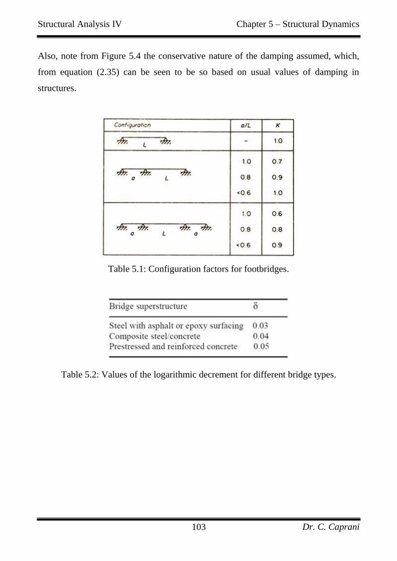
Structural Analysis IV Chapter 5 – Structural Dynamics
Dr. C. Caprani 103
Also, note from Figure 5.4 the conservative nature of the damping assumed, which,
from equation (2.35) can be seen to be so based on usual values of damping in
structures.
Table 5.1: Configuration factors for footbridges.
Table 5.2: Values of the logarithmic decrement for different bridge types.
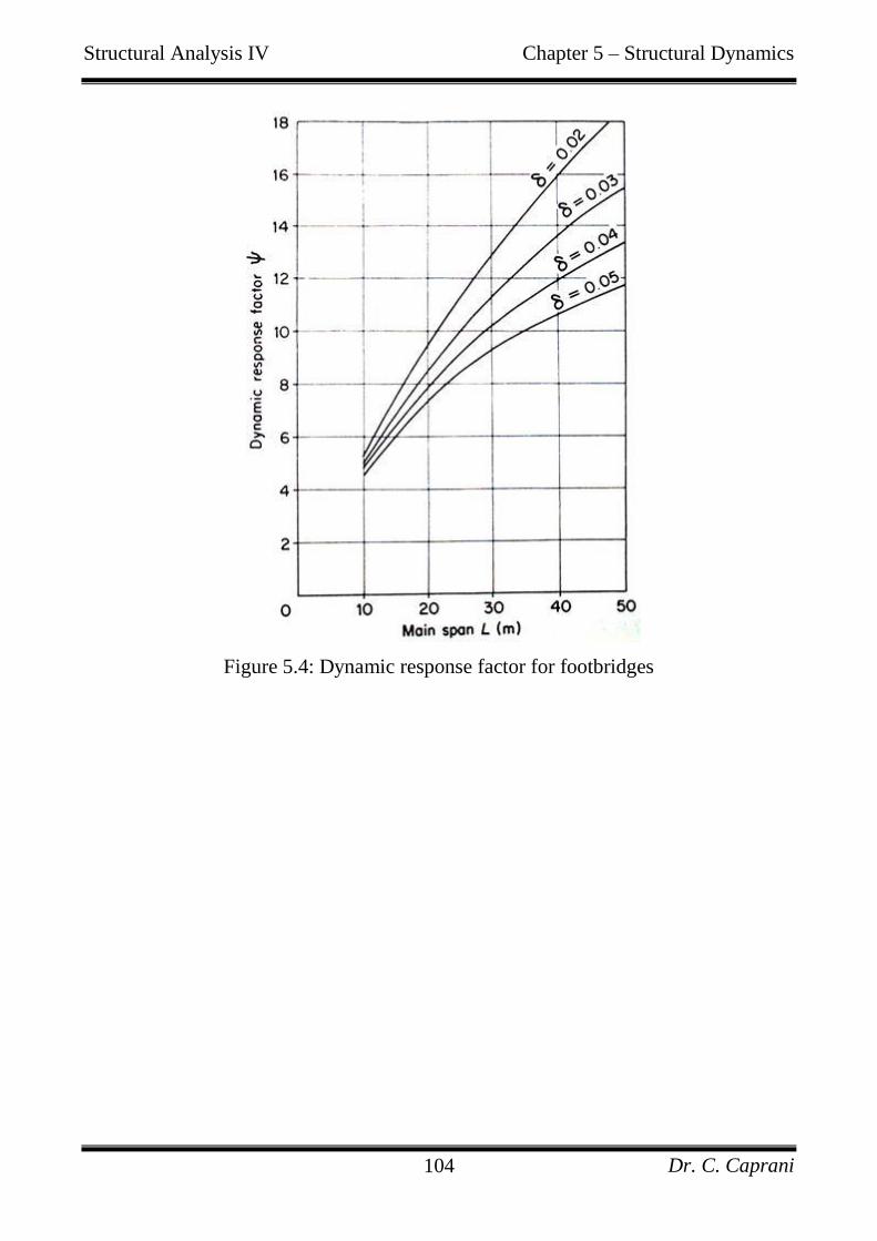
Structural Analysis IV Chapter 5 – Structural Dynamics
Dr. C. Caprani 104
Figure 5.4: Dynamic response factor for footbridges
Structural Analysis IV Chapter 5 – Structural Dynamics
Dr. C. Caprani 105
Design Example
A simply-supported footbridge of 18 m span has a total mass of 12.6 tonnes and
flexural stiffness of 3×10⁵ kNm
2. Determine the maximum amplitude of vibration and
vertical acceleration caused by a 0.7 kN pedestrian walking in frequency with the
bridge: the pedestrian has a stride of 0.9 m and produces an effective pulsating force
of 180 N. Assume the damping to be related to 0.05 . Is this a comfortable bridge
for the pedestrian (Figure 5.1)?
The natural frequency of the bridge is, from equations (2.19) and (4.21):
8
2
3 103.17 Hz
2 18 12600/18f
The static deflection is:
3
8
700 180.2835 mm
48 3 10st
u
Table 5.1 gives 1K and Figure 5.4 gives 6.8 and so, by (5.5.2) we have:
max
0.2835 1.0 6.8 1.93 mmu
and so the maximum acceleration is:
22 3 2
max max2 3.17 1.93 10 0.78 m/su u
We compare this to the requirement that:
Structural Analysis IV Chapter 5 – Structural Dynamics
Dr. C. Caprani 106
max
2
0.5
0.5
0.78 0.89 m/s
u f
f
And so we deem the bridge acceptable. From Figure 5.1, with the amplitude 1.93 mm
and 3.17 Hz frequency, we can see that this pedestrian will feel decidedly
uncomfortable and will probably change pace to avoid this frequency of loading.
The above discussion, in conjunction with Section 2.d reveals why, historically,
soldiers were told to break step when crossing a slender bridge – unfortunately for
some, it is more probable that this knowledge did not come from any detailed
dynamic analysis; rather, bitter experience.
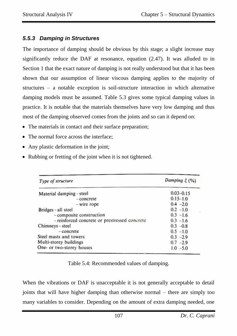
Structural Analysis IV Chapter 5 – Structural Dynamics
Dr. C. Caprani 107
5.5.3 Damping in Structures
The importance of damping should be obvious by this stage; a slight increase may
significantly reduce the DAF at resonance, equation (2.47). It was alluded to in
Section 1 that the exact nature of damping is not really understood but that it has been
shown that our assumption of linear viscous damping applies to the majority of
structures – a notable exception is soil-structure interaction in which alternative
damping models must be assumed. Table 5.3 gives some typical damping values in
practice. It is notable that the materials themselves have very low damping and thus
most of the damping observed comes from the joints and so can it depend on:
The materials in contact and their surface preparation;
The normal force across the interface;
Any plastic deformation in the joint;
Rubbing or fretting of the joint when it is not tightened.
Table 5.4: Recommended values of damping.
When the vibrations or DAF is unacceptable it is not generally acceptable to detail
joints that will have higher damping than otherwise normal – there are simply too
many variables to consider. Depending on the amount of extra damping needed, one
Structural Analysis IV Chapter 5 – Structural Dynamics
Dr. C. Caprani 108
could wait for the structure to be built and then measure the damping, retro-fitting
vibration isolation devices as required. Or, if the extra damping required is
significant, the design of a vibration isolation device may be integral to the structure.
The devices that may be installed vary; some are:
Tuned mass dampers (TMDs): a relatively small mass is attached to the primary
system and is „tuned‟ to vibrate at the same frequency but to oppose the primary
system;
Sloshing dampers: A large water tank is used – the sloshing motion opposes the
primary system motion due to inertial effects;
Liquid column dampers: Two columns of liquid, connected at their bases but at
opposite sides of the primary system slosh, in a more controlled manner to oppose
the primary system motion.
These are the approaches taken in many modern buildings, particularly in Japan and
other earthquake zones. The Citicorp building in New York (which is famous for
other reasons also) and the John Hancock building in Boston were among the first to
use TMDs. In the John Hancock building a concrete block of about 300 tonnes
located on the 54th storey sits on a thin film of oil. When the building sways the
inertial effects of the block mean that it moves in the opposite direction to that of the
sway and so opposes the motion (relying heavily on a lack of friction). This is quite a
rudimentary system compared to modern systems which have computer controlled
actuators that take input from accelerometers in the building and move the block an
appropriate amount.
Structural Analysis IV Chapter 5 – Structural Dynamics
Dr. C. Caprani 109
5.5.4 Design Rules of Thumb
General
The structure should not have any modal frequency close to the frequency of any
form of periodic loading, irrespective of magnitude. This is based upon the large
DAFs that may occur (Section 2.d).
For normal floors of span/depth ratio less than 25 vibration is not generally a
problem. Problematic floors are lightweight with spans of over about 7 m.
Human loading
Most forms of human loading occur at frequencies < 5 Hz (Sections 1 and 5.a) and so
any structure of natural frequency greater than this should not be subject to undue
dynamic excitation.
Machine Loading
By avoiding any of the frequencies that the machine operates at, vibrations may be
minimised. The addition of either more stiffness or mass will change the frequencies
the structure responds to. If the response is still not acceptable vibration isolation
devices may need to be considered (Section 5.c).
Approximate Frequencies
The Bolton Method of Section 4.b is probably the best for those structures outside the
standard cases of Section 4.a. Careful thought on reducing the size of the problem to
an SDOF system usually enables good approximate analysis.
Other methods are:
Structural Analysis IV Chapter 5 – Structural Dynamics
Dr. C. Caprani 110
Structures with concentrated mass: 1
2
gf
Simplified rule for most structures: 18
f
where is the static deflection and g is the acceleration under gravity.
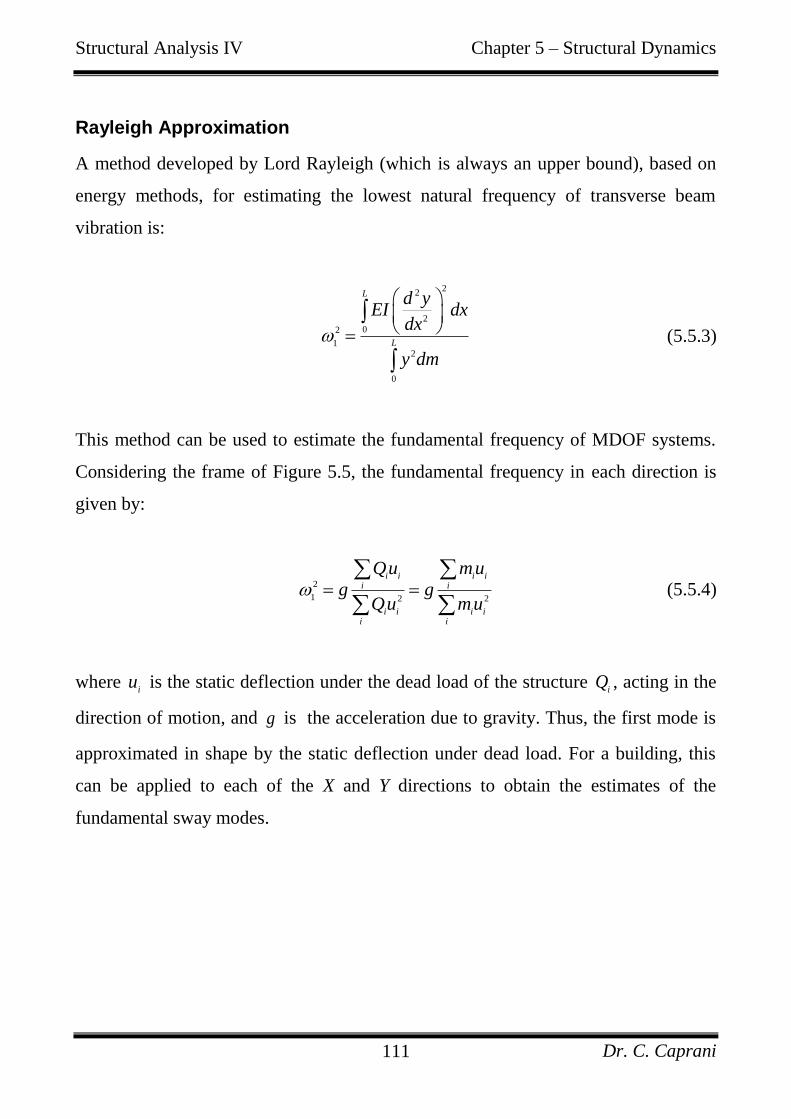
Structural Analysis IV Chapter 5 – Structural Dynamics
Dr. C. Caprani 111
Rayleigh Approximation
A method developed by Lord Rayleigh (which is always an upper bound), based on
energy methods, for estimating the lowest natural frequency of transverse beam
vibration is:
22
2
02
12
0
L
L
d yEI dx
dx
y dm
(5.5.3)
This method can be used to estimate the fundamental frequency of MDOF systems.
Considering the frame of Figure 5.5, the fundamental frequency in each direction is
given by:
2
1 2 2
i i i ii i
i i i ii i
Qu mu
g gQu mu
(5.5.4)
where i
u is the static deflection under the dead load of the structure i
Q , acting in the
direction of motion, and g is the acceleration due to gravity. Thus, the first mode is
approximated in shape by the static deflection under dead load. For a building, this
can be applied to each of the X and Y directions to obtain the estimates of the
fundamental sway modes.
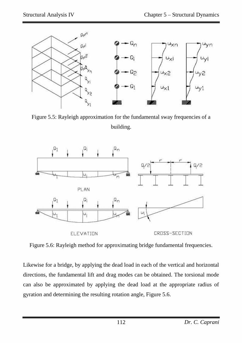
Structural Analysis IV Chapter 5 – Structural Dynamics
Dr. C. Caprani 112
Figure 5.5: Rayleigh approximation for the fundamental sway frequencies of a
building.
Figure 5.6: Rayleigh method for approximating bridge fundamental frequencies.
Likewise for a bridge, by applying the dead load in each of the vertical and horizontal
directions, the fundamental lift and drag modes can be obtained. The torsional mode
can also be approximated by applying the dead load at the appropriate radius of
gyration and determining the resulting rotation angle, Figure 5.6.

Structural Analysis IV Chapter 5 – Structural Dynamics
Dr. C. Caprani 113
This method is particularly useful when considering the results of a detailed analysis,
such as finite-element. It provides a reasonable approximate check on the output.

Structural Analysis IV Chapter 5 – Structural Dynamics
Dr. C. Caprani 114
5.6 Appendix
5.6.1 Past Exam Questions
Summer 2005
Question 5
(a) The system shown in Figure Q.5(a) is known to have a static deflection of 32.7 mm for an unknown mass.
1) Find the natural frequency of the system.
(10%)
2) Given that the mass is 10 kg, find the peak displacement when this mass is given an initial
velocity of 500 mm/s and an initial displacement of 25 mm.
(10%)
3) What time does the first positive peak occur?
(10%)
4) What value of damping coefficient is required such that the amplitude after 5 oscillations is 10%
of the first peak?
(10%)
5) What is the peak force in the spring?
(20%)
(b) A cantilever riverside boardwalk has been opened to the public as shown in Figure Q.5(b); however, it was
found that the structure experiences significant human- and traffic-induced vibrations. An harmonic
oscillation test found the natural frequency of the structure to be 2.25 Hz. It is proposed to retro-fit braced
struts at 5m spacings so that the natural period of vibration will be 9 Hz – given E = 200 kN/mm2 and
ignoring buckling effects, what area of strut is required?
(40%)
Ans. (a) 2.756 Hz; 38.2 mm; 0.05 s; 99 kg.s/m;114.5 N; (b) 67.5 mm2.
FIG. Q.5(b)
m
k
FIG. Q.5(a)
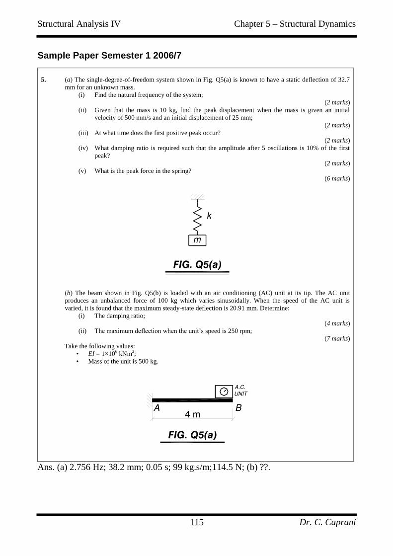
Structural Analysis IV Chapter 5 – Structural Dynamics
Dr. C. Caprani 115
Sample Paper Semester 1 2006/7
5. (a) The single-degree-of-freedom system shown in Fig. Q5(a) is known to have a static deflection of 32.7
mm for an unknown mass.
(i) Find the natural frequency of the system;
(2 marks)
(ii) Given that the mass is 10 kg, find the peak displacement when the mass is given an initial
velocity of 500 mm/s and an initial displacement of 25 mm;
(2 marks)
(iii) At what time does the first positive peak occur?
(2 marks)
(iv) What damping ratio is required such that the amplitude after 5 oscillations is 10% of the first
peak?
(2 marks)
(v) What is the peak force in the spring?
(6 marks)
(b) The beam shown in Fig. Q5(b) is loaded with an air conditioning (AC) unit at its tip. The AC unit
produces an unbalanced force of 100 kg which varies sinusoidally. When the speed of the AC unit is
varied, it is found that the maximum steady-state deflection is 20.91 mm. Determine:
(i) The damping ratio;
(4 marks)
(ii) The maximum deflection when the unit‟s speed is 250 rpm;
(7 marks)
Take the following values:
• EI = 1×10⁶ kNm
2;
• Mass of the unit is 500 kg.
Ans. (a) 2.756 Hz; 38.2 mm; 0.05 s; 99 kg.s/m;114.5 N; (b) ??.
FIG. Q5(a)
FIG. Q5(a)
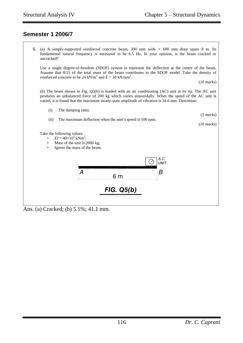
Structural Analysis IV Chapter 5 – Structural Dynamics
Dr. C. Caprani 116
Semester 1 2006/7
5. (a) A simply-supported reinforced concrete beam, 300 mm wide × 600 mm deep spans 8 m. Its
fundamental natural frequency is measured to be 6.5 Hz. In your opinion, is the beam cracked or
uncracked?
Use a single degree-of-freedom (SDOF) system to represent the deflection at the centre of the beam.
Assume that 8/15 of the total mass of the beam contributes to the SDOF model. Take the density of
reinforced concrete to be 24 kN/m3 and E = 30 kN/mm
2.
(10 marks)
(b) The beam shown in Fig. Q5(b) is loaded with an air conditioning (AC) unit at its tip. The AC unit
produces an unbalanced force of 200 kg which varies sinusoidally. When the speed of the AC unit is
varied, it is found that the maximum steady-state amplitude of vibration is 34.6 mm. Determine:
(i) The damping ratio;
(5 marks)
(ii) The maximum deflection when the unit‟s speed is 100 rpm;
(10 marks)
Take the following values:
• EI = 40×103 kNm
2;
• Mass of the unit is 2000 kg;
• Ignore the mass of the beam.
Ans. (a) Cracked; (b) 5.1%; 41.1 mm.
FIG. Q5(a)
FIG. Q5(b)
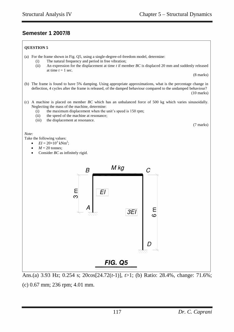
Structural Analysis IV Chapter 5 – Structural Dynamics
Dr. C. Caprani 117
Semester 1 2007/8
QUESTION 5
(a) For the frame shown in Fig. Q5, using a single-degree-of-freedom model, determine:
(i) The natural frequency and period in free vibration;
(ii) An expression for the displacement at time t if member BC is displaced 20 mm and suddenly released
at time t = 1 sec.
(8 marks)
(b) The frame is found to have 5% damping. Using appropriate approximations, what is the percentage change in
deflection, 4 cycles after the frame is released, of the damped behaviour compared to the undamped behaviour?
(10 marks)
(c) A machine is placed on member BC which has an unbalanced force of 500 kg which varies sinusoidally.
Neglecting the mass of the machine, determine:
(i) the maximum displacement when the unit‟s speed is 150 rpm;
(ii) the speed of the machine at resonance;
(iii) the displacement at resonance.
(7 marks)
Note:
Take the following values:
EI = 20×103 kNm
2;
M = 20 tonnes;
Consider BC as infinitely rigid.
Ans.(a) 3.93 Hz; 0.254 s; 20cos[24.72(t-1)], t>1; (b) Ratio: 28.4%, change: 71.6%;
(c) 0.67 mm; 236 rpm; 4.01 mm.
FIG. Q5
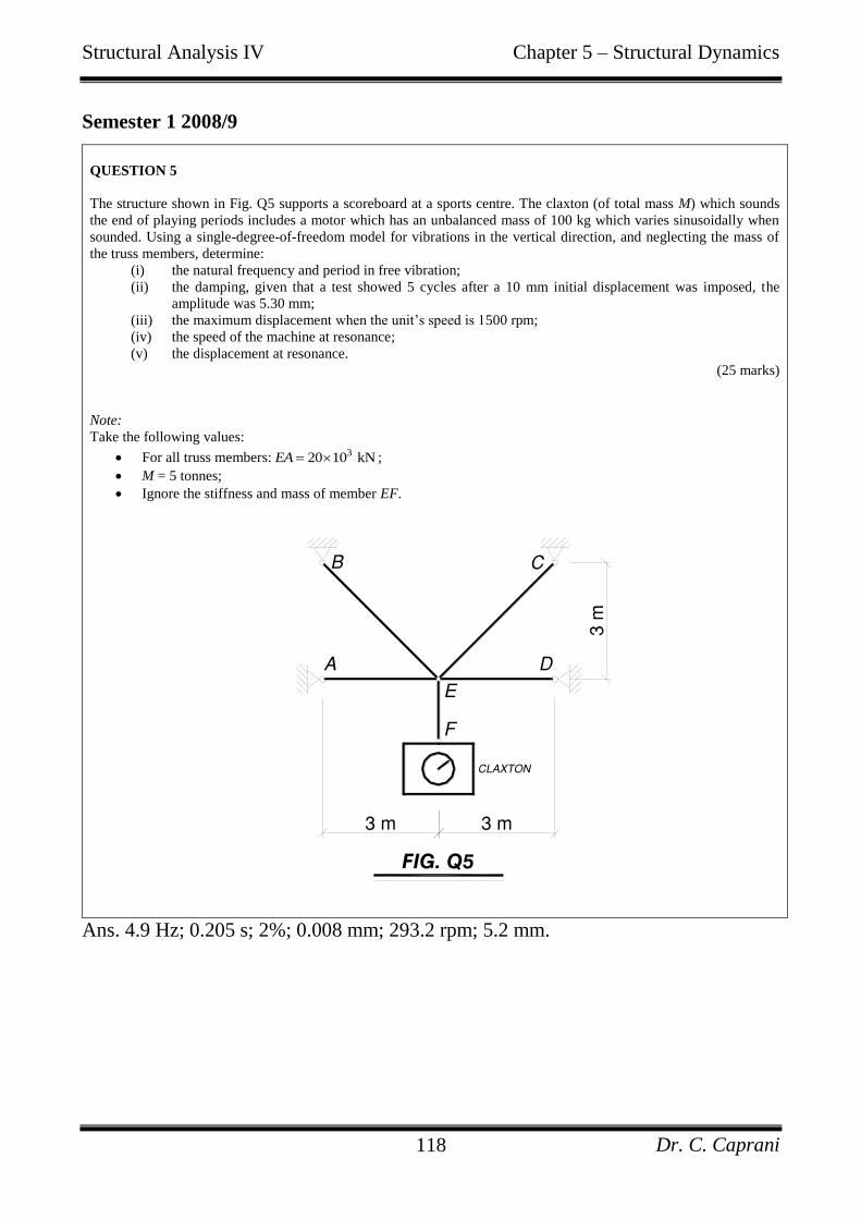
Structural Analysis IV Chapter 5 – Structural Dynamics
Dr. C. Caprani 118
Semester 1 2008/9
QUESTION 5
The structure shown in Fig. Q5 supports a scoreboard at a sports centre. The claxton (of total mass M) which sounds
the end of playing periods includes a motor which has an unbalanced mass of 100 kg which varies sinusoidally when
sounded. Using a single-degree-of-freedom model for vibrations in the vertical direction, and neglecting the mass of
the truss members, determine:
(i) the natural frequency and period in free vibration;
(ii) the damping, given that a test showed 5 cycles after a 10 mm initial displacement was imposed, the
amplitude was 5.30 mm;
(iii) the maximum displacement when the unit‟s speed is 1500 rpm;
(iv) the speed of the machine at resonance;
(v) the displacement at resonance.
(25 marks)
Note:
Take the following values:
For all truss members: 320 10 kNEA ;
M = 5 tonnes;
Ignore the stiffness and mass of member EF.
Ans. 4.9 Hz; 0.205 s; 2%; 0.008 mm; 293.2 rpm; 5.2 mm.
FIG. Q5
Structural Analysis IV Chapter 5 – Structural Dynamics
Dr. C. Caprani 119
Semester 1 2009/10
QUESTION 5
(a) A 3 m high, 6 m wide single-bay single-storey frame is rigidly jointed with a beam of mass 2,000 kg and columns
of negligible mass and stiffness of 3 22.7 10 kNmEI . Assuming the beam to be infinitely rigid, calculate the
natural frequency in lateral vibration and its period. Find the force required to deflect the frame 20 mm laterally.
(10 marks)
(b) A spring-mass-damper SDOF system is subject to a harmonically varying force. At resonance, the amplitude of
vibration is found to be 10 mm, and at 0.80 of the resonant frequency, the amplitude is found to be 5.07 mm.
Determine the damping of the system.
(15 marks)
Ans. 5.51 Hz, 48 kN.; 0.1.
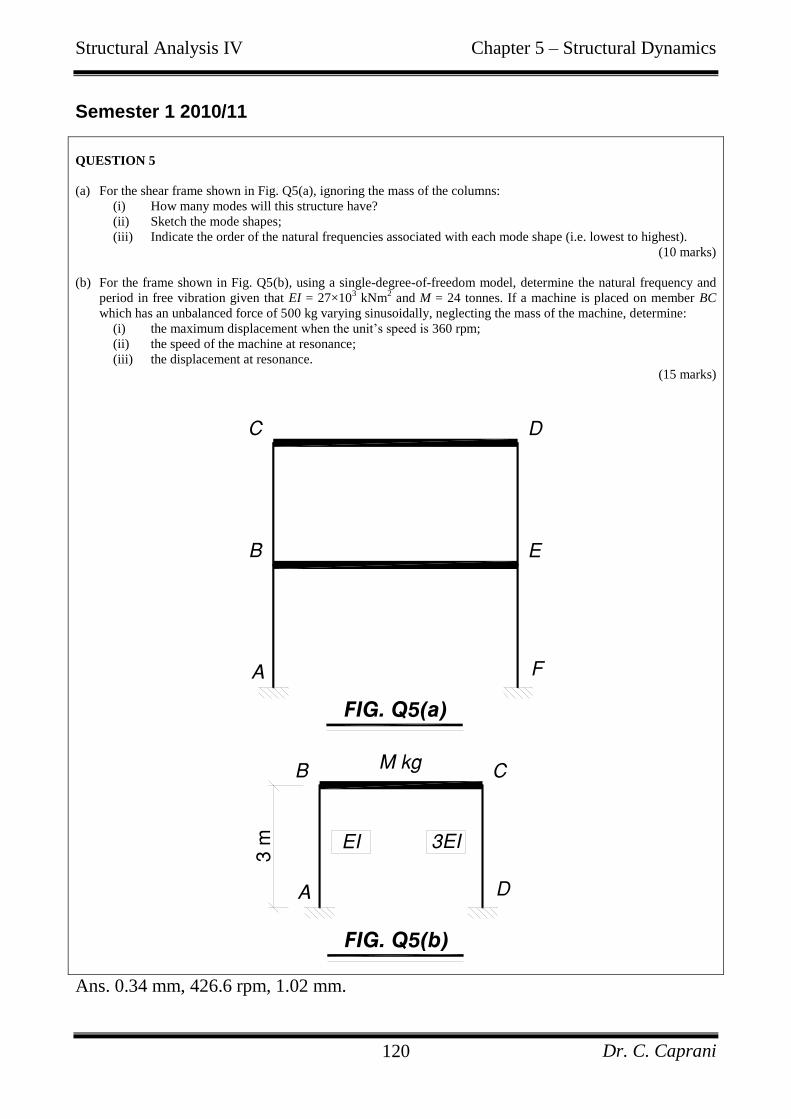
Structural Analysis IV Chapter 5 – Structural Dynamics
Dr. C. Caprani 120
Semester 1 2010/11
QUESTION 5
(a) For the shear frame shown in Fig. Q5(a), ignoring the mass of the columns:
(i) How many modes will this structure have?
(ii) Sketch the mode shapes;
(iii) Indicate the order of the natural frequencies associated with each mode shape (i.e. lowest to highest).
(10 marks)
(b) For the frame shown in Fig. Q5(b), using a single-degree-of-freedom model, determine the natural frequency and
period in free vibration given that EI = 27×103 kNm
2 and M = 24 tonnes. If a machine is placed on member BC
which has an unbalanced force of 500 kg varying sinusoidally, neglecting the mass of the machine, determine:
(i) the maximum displacement when the unit‟s speed is 360 rpm;
(ii) the speed of the machine at resonance;
(iii) the displacement at resonance.
(15 marks)
Ans. 0.34 mm, 426.6 rpm, 1.02 mm.
FIG. Q5(a)
FIG. Q5(b)
Structural Analysis IV Chapter 5 – Structural Dynamics
Dr. C. Caprani 121
5.6.2 References
The following books/articles were referred to in the writing of these notes;
particularly Clough & Penzien (1993), Smith (1988) and Bolton (1978) - these should
be referred to first for more information. There is also a lot of information and
software available online; the software can especially help intuitive understanding.
The class notes of Mr. R. Mahony (D.I.T.) and Dr. P. Fanning (U.C.D.) were also
used.
Archbold, P., (2002), “Modal Analysis of a GRP Cable-Stayed Bridge”,
Proceedings of the First Symposium of Bridge Engineering Research In Ireland,
Eds. C. McNally & S. Brady, University College Dublin.
Beards, C.F., (1983), Structural Vibration Analysis: modelling, analysis and
damping of vibrating structures, Ellis Horwood, Chichester, England.
Bhatt, P., (1999), Structures, Longman, Harlow, England.
Bolton, A., (1978), “Natural frequencies of structures for designers”, The
Structural Engineer, Vol. 56A, No. 9, pp. 245-253; Discussion: Vol. 57A, No. 6,
p.202, 1979.
Bolton, A., (1969), “The natural frequencies of continuous beams”, The Structural
Engineer, Vol. 47, No. 6, pp.233-240.
Case, J., Chilver, A.H. and Ross, C.T.F., (1999), Strength of Materials and
Structures, 4th edn., Arnold, London.
Chopra, A.K., (2007), Dynamics of Structures – Theory and Applications to
Earthquake Engineering, 3rd edn., Pearson-Prentice Hall, New Jersey.
Clough, R.W. and Penzien, J., (1993), Dynamics of Structures, 2nd edn., McGraw-
Hill, New York.
Cobb, F. (2004), Structural Engineer’s Pocket Book, Elsevier, Oxford.
Craig, R.R., (1981), Structural Dynamics – An introduction to computer methods,
Wiley, New York.
Structural Analysis IV Chapter 5 – Structural Dynamics
Dr. C. Caprani 122
Ghali, A. and Neville, A.M., (1997), Structural Analysis – A unified classical and
matrix approach, 4th edn., E&FN Spon, London.
Irvine, M., (1986), Structural Dynamics for the Practising Engineer, Allen &
Unwin, London.
Kreyszig, E., (1993), Advanced Engineering Mathematics, 7th edn., Wiley.
Paz, M. and Leigh, W., (2004), Structural Dynamics – Theory and Computation,
5th edn., Springer, New York.
Smith, J.W., (1988), Vibration of Structures – Applications in civil engineering
design, Chapman and Hall, London.
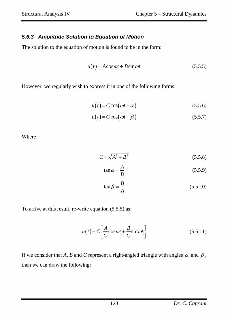
Structural Analysis IV Chapter 5 – Structural Dynamics
Dr. C. Caprani 123
5.6.3 Amplitude Solution to Equation of Motion
The solution to the equation of motion is found to be in the form:
cos sinu t A t B t (5.5.5)
However, we regularly wish to express it in one of the following forms:
cosu t C t (5.5.6)
cosu t C t (5.5.7)
Where
2 2C A B (5.5.8)
tanA
B (5.5.9)
tanB
A (5.5.10)
To arrive at this result, re-write equation (5.5.5) as:
cos sinA B
u t C t tC C
(5.5.11)
If we consider that A, B and C represent a right-angled triangle with angles and ,
then we can draw the following:
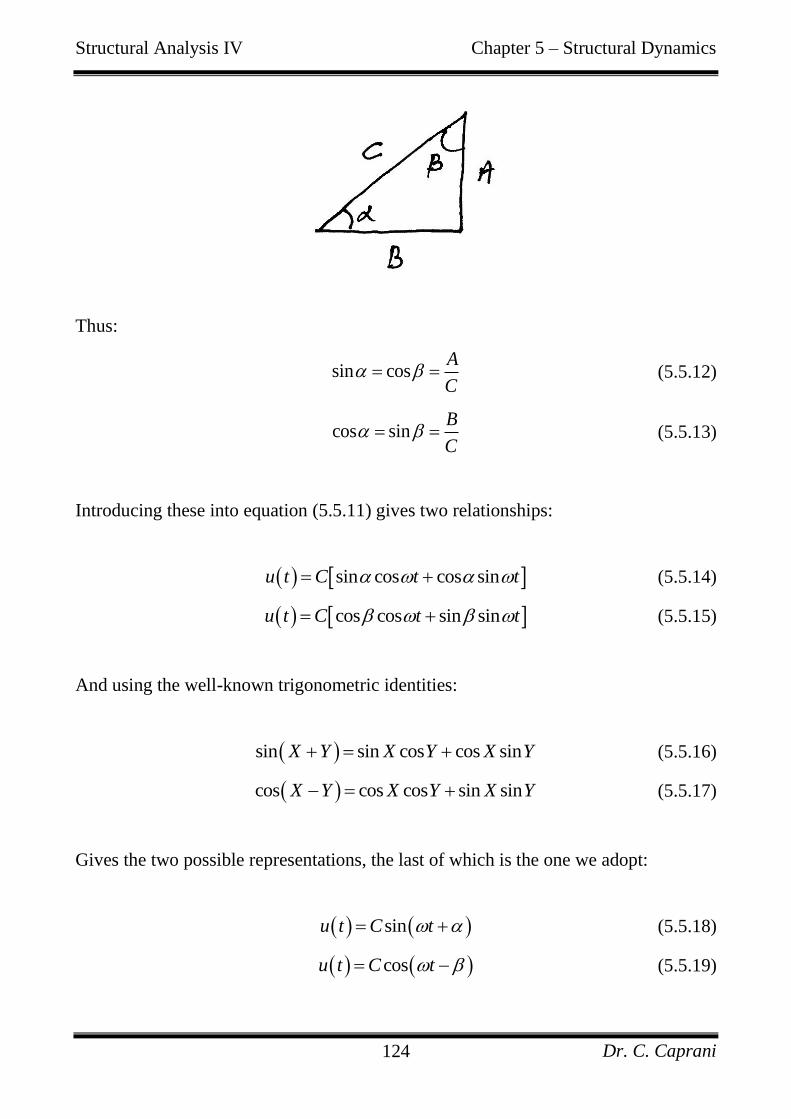
Structural Analysis IV Chapter 5 – Structural Dynamics
Dr. C. Caprani 124
Thus:
sin cosA
C (5.5.12)
cos sinB
C (5.5.13)
Introducing these into equation (5.5.11) gives two relationships:
sin cos cos sinu t C t t (5.5.14)
cos cos sin sinu t C t t (5.5.15)
And using the well-known trigonometric identities:
sin sin cos cos sinX Y X Y X Y (5.5.16)
cos cos cos sin sinX Y X Y X Y (5.5.17)
Gives the two possible representations, the last of which is the one we adopt:
sinu t C t (5.5.18)
cosu t C t (5.5.19)
Structural Analysis IV Chapter 5 – Structural Dynamics
Dr. C. Caprani 125
5.6.4 Solutions to Differential Equations
The Homogenous Equation
To find the solution of:
2
2
20
d yk y
dx (5.5.20)
we try xy e (note that this k has nothing to do with stiffness but is the conventional
mathematical notation for this problem). Thus we have:
2
2
2;x xdy d y
e edx dx
Substituting this into (5.5.20) gives:
2 2 0x xe k e
And so we get the characteristic equation by dividing out xe :
2 2 0k
From which:
2k
Or,
Structural Analysis IV Chapter 5 – Structural Dynamics
Dr. C. Caprani 126
1 2
;ik ik
Where 1i . Since these are both solutions, they are both valid and the expression
for y becomes:
1 2
ikx ikxy Ae A e (5.5.21)
In which 1
A and 2
A are constants to be determined from the initial conditions of the
problem. Introducing Euler‟s equations:
cos sin
cos sin
ikx
ikx
e kx i kx
e kx i kx
(5.5.22)
into (5.5.21) gives us:
1 2cos sin cos siny A kx i kx A kx i kx
Collecting terms:
1 2 1 2cos siny A A kx iA iA kx
Since the coefficients of the trigonometric functions are constants we can just write:
cos siny A kx B kx (5.5.23)
Structural Analysis IV Chapter 5 – Structural Dynamics
Dr. C. Caprani 127
The Non-homogenous Equation
Starting with equation (5.2.47) (repeated here for convenience):
0
( ) ( ) ( ) sinmu t cu t ku t F t (5.5.24)
We divide by m and introduce equations (5.2.10) and (5.2.12) to get:
2 0( ) 2 ( ) ( ) sin
Fu t u t u t t
m (5.5.25)
At this point, recall that the solution to non-homogenous differential equations is
made up of two parts:
The complimentary solution ( Cu t ): this is the solution to the corresponding
homogenous equation, which we already have (equation (5.5.23));
The particular solution ( Pu t ): particular to the function on the right hand side
of equation (5.5.24), which we must now find.
The final solution is the sum of the complimentary and particular solutions:
C Pu t u t u t (5.5.26)
For the particular solution we try the following:
sin cosP
u t C t D t (5.5.27)
Then we have:
cos sinP
u t C t D t (5.5.28)
Structural Analysis IV Chapter 5 – Structural Dynamics
Dr. C. Caprani 128
And
2 2sin cosP
u t C t D t (5.5.29)
Substituting equations (5.5.27), (5.5.28) and (5.5.29) into equation (5.5.25) gives:
2 2
2 0
sin cos
2 cos sin
sin cos sin
C t D t
C t D t
FC t D t t
m
(5.5.30)
Collecting sine and cosine terms:
2 2
2 2 0
2 sin
2 cos sin
C D t
FC D t t
m
(5.5.31)
For this to be valid for all t, the sine and cosine terms on both sides of the equation
must be equal. Thus:
2 2 02F
C Dm
(5.5.32)
2 22 0C D (5.5.33)
Next, divide both sides by 2 :
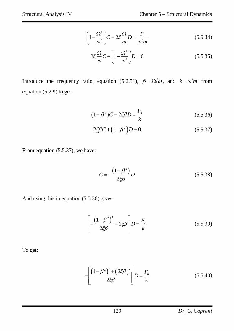
Structural Analysis IV Chapter 5 – Structural Dynamics
Dr. C. Caprani 129
2
0
2 21 2
FC D
m
(5.5.34)
2
22 1 0C D
(5.5.35)
Introduce the frequency ratio, equation (5.2.51), , and 2k m from
equation (5.2.9) to get:
2 01 2F
C Dk
(5.5.36)
22 1 0C D (5.5.37)
From equation (5.5.37), we have:
21
2C D
(5.5.38)
And using this in equation (5.5.36) gives:
22
01
22
FD
k
(5.5.39)
To get:
2 22
01 2
2
FD
k
(5.5.40)
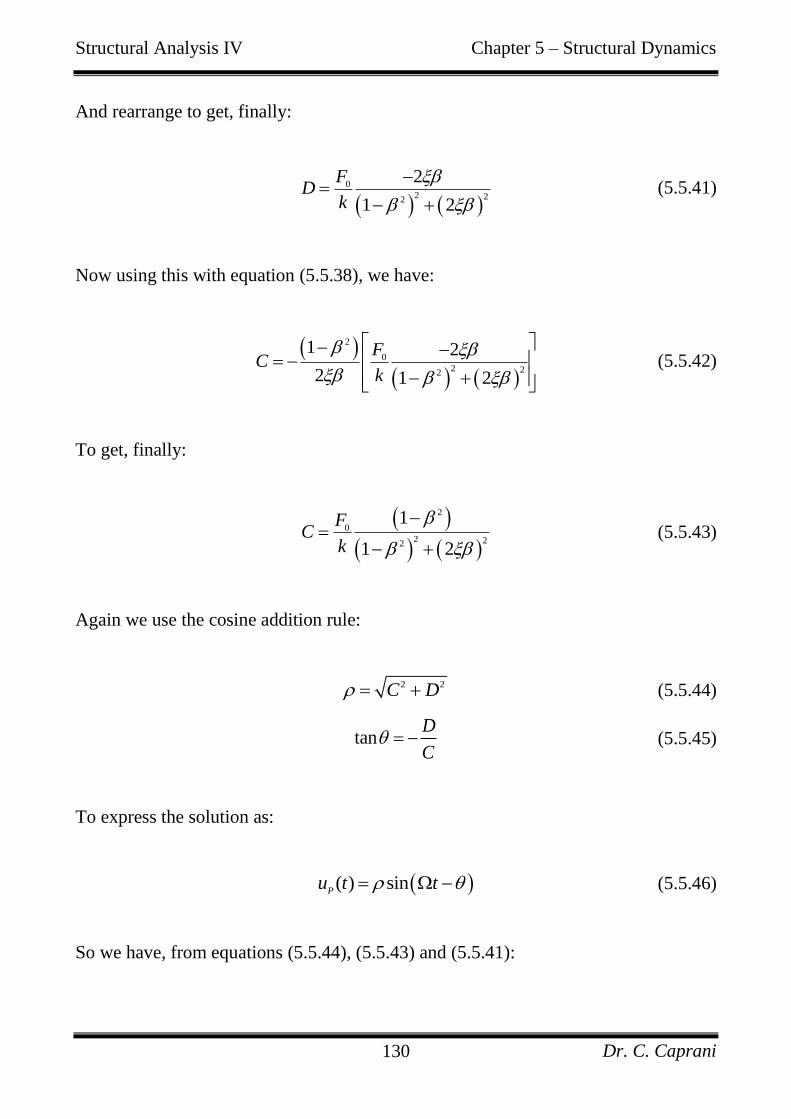
Structural Analysis IV Chapter 5 – Structural Dynamics
Dr. C. Caprani 130
And rearrange to get, finally:
0
2 22
2
1 2
FD
k
(5.5.41)
Now using this with equation (5.5.38), we have:
2
0
2 22
1 2
2 1 2
FC
k
(5.5.42)
To get, finally:
2
0
2 22
1
1 2
FC
k
(5.5.43)
Again we use the cosine addition rule:
2 2C D (5.5.44)
tanD
C (5.5.45)
To express the solution as:
( ) sinP
u t t (5.5.46)
So we have, from equations (5.5.44), (5.5.43) and (5.5.41):
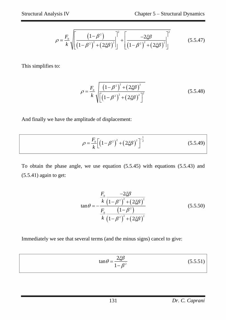
Structural Analysis IV Chapter 5 – Structural Dynamics
Dr. C. Caprani 131
2 22
0
2 22 22 2
1 2
1 2 1 2
F
k
(5.5.47)
This simplifies to:
2 22
0
22 22
1 2
1 2
F
k
(5.5.48)
And finally we have the amplitude of displacement:
1
2 2 220 1 2F
k
(5.5.49)
To obtain the phase angle, we use equation (5.5.45) with equations (5.5.43) and
(5.5.41) again to get:
0
2 22
2
0
2 22
2
1 2tan
1
1 2
F
k
F
k
(5.5.50)
Immediately we see that several terms (and the minus signs) cancel to give:
2
2tan
1
(5.5.51)
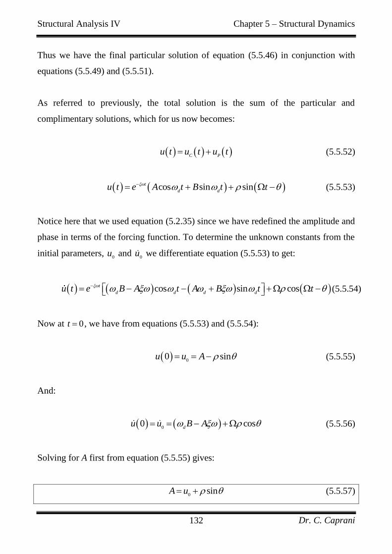
Structural Analysis IV Chapter 5 – Structural Dynamics
Dr. C. Caprani 132
Thus we have the final particular solution of equation (5.5.46) in conjunction with
equations (5.5.49) and (5.5.51).
As referred to previously, the total solution is the sum of the particular and
complimentary solutions, which for us now becomes:
C Pu t u t u t (5.5.52)
cos sin sint
d du t e A t B t t (5.5.53)
Notice here that we used equation (5.2.35) since we have redefined the amplitude and
phase in terms of the forcing function. To determine the unknown constants from the
initial parameters, 0
u and 0
u we differentiate equation (5.5.53) to get:
cos sin cost
d d d du t e B A t A B t t (5.5.54)
Now at 0t , we have from equations (5.5.53) and (5.5.54):
00 sinu u A (5.5.55)
And:
00 cos
du u B A (5.5.56)
Solving for A first from equation (5.5.55) gives:
0
sinA u (5.5.57)
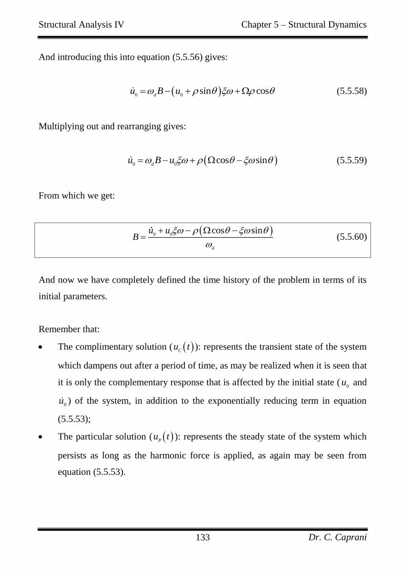
Structural Analysis IV Chapter 5 – Structural Dynamics
Dr. C. Caprani 133
And introducing this into equation (5.5.56) gives:
0 0sin cos
du B u (5.5.58)
Multiplying out and rearranging gives:
0 0cos sin
du B u (5.5.59)
From which we get:
0 0
cos sin
d
u uB
(5.5.60)
And now we have completely defined the time history of the problem in terms of its
initial parameters.
Remember that:
The complimentary solution ( Cu t ): represents the transient state of the system
which dampens out after a period of time, as may be realized when it is seen that
it is only the complementary response that is affected by the initial state (0
u and
0u ) of the system, in addition to the exponentially reducing term in equation
(5.5.53);
The particular solution ( Pu t ): represents the steady state of the system which
persists as long as the harmonic force is applied, as again may be seen from
equation (5.5.53).
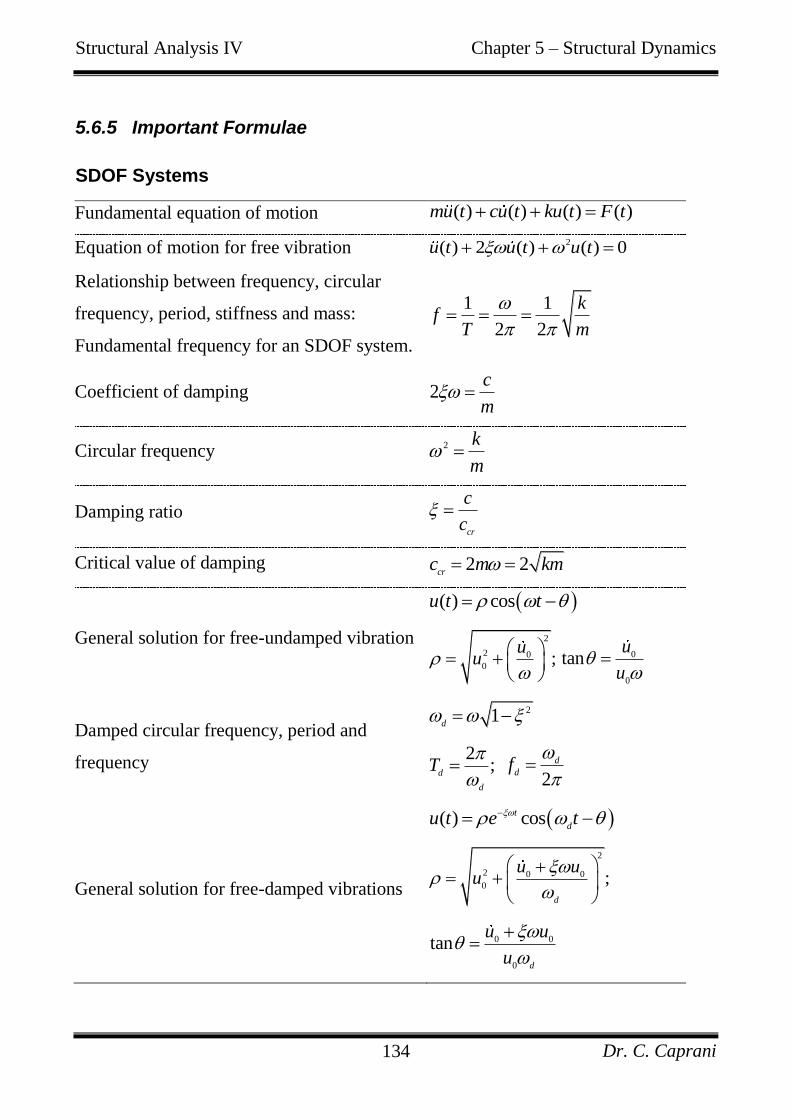
Structural Analysis IV Chapter 5 – Structural Dynamics
Dr. C. Caprani 134
5.6.5 Important Formulae
SDOF Systems
Fundamental equation of motion ( ) ( ) ( ) ( )mu t cu t ku t F t
Equation of motion for free vibration 2( ) 2 ( ) ( ) 0u t u t u t
Relationship between frequency, circular
frequency, period, stiffness and mass:
Fundamental frequency for an SDOF system.
1 1
2 2
kf
T m
Coefficient of damping 2c
m
Circular frequency 2 k
m
Damping ratio cr
c
c
Critical value of damping 2 2cr
c m km
General solution for free-undamped vibration
( ) cosu t t
2
2 0
0;
uu
0
0
tanu
u
Damped circular frequency, period and
frequency
21d
2;
d
d
T
2
d
df
General solution for free-damped vibrations
( ) cost
du t e t
2
2 0 0
0;
d
u uu
0 0
0
tand
u u
u
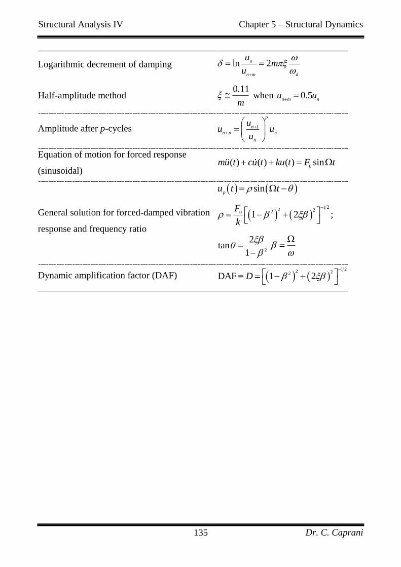
Structural Analysis IV Chapter 5 – Structural Dynamics
Dr. C. Caprani 135
Logarithmic decrement of damping ln 2n
n m d
um
u
Half-amplitude method 0.11
m when 0.5
n m nu u
Amplitude after p-cycles 1
p
n
n p n
n
uu u
u
Equation of motion for forced response
(sinusoidal) 0
( ) ( ) ( ) sinmu t cu t ku t F t
General solution for forced-damped vibration
response and frequency ratio
sinp
u t t
1 2
2 220 1 2 ;F
k
2
2tan
1
Dynamic amplification factor (DAF) 1 2
2 22DAF 1 2D
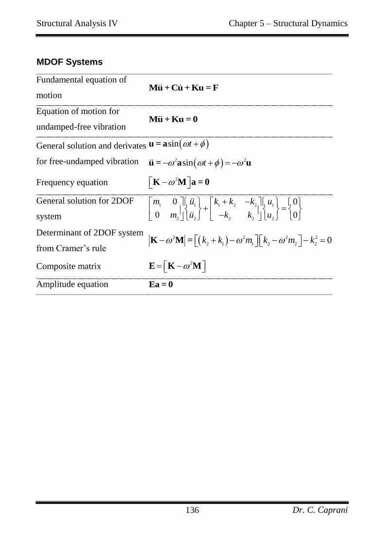
Structural Analysis IV Chapter 5 – Structural Dynamics
Dr. C. Caprani 136
MDOF Systems
Fundamental equation of
motion Mu + Cu + Ku = F
Equation of motion for
undamped-free vibration Mu + Ku = 0
General solution and derivates
for free-undamped vibration
sin t u = a
2 2sin t u = a u
Frequency equation 2 K M a = 0
General solution for 2DOF
system
1 1 1 2 2 1
2 2 2 2 2
0 0
0 0
m u k k k u
m u k k u
Determinant of 2DOF system
from Cramer‟s rule 2 2 2 2
2 1 1 2 2 20k k m k m k K M =
Composite matrix 2 E K M
Amplitude equation Ea = 0
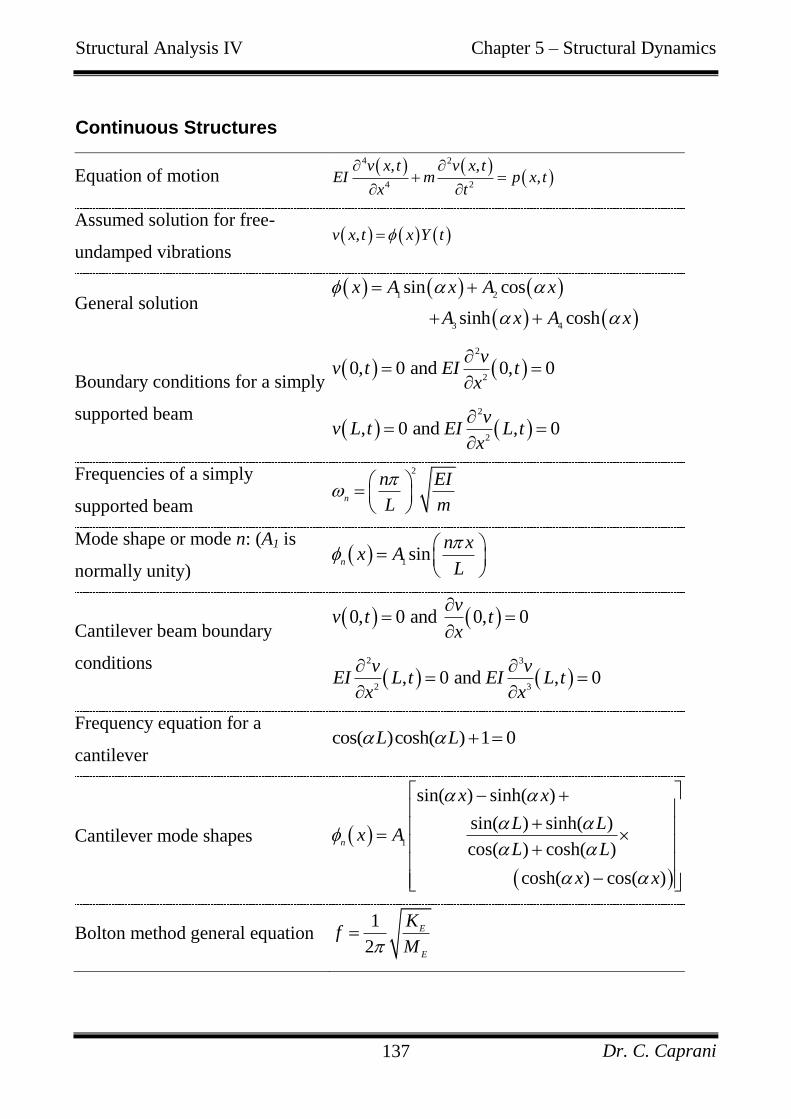
Structural Analysis IV Chapter 5 – Structural Dynamics
Dr. C. Caprani 137
Continuous Structures
Equation of motion
Assumed solution for free-
undamped vibrations
General solution
1 2
3 4
sin cos
sinh cosh
x A x A x
A x A x
Boundary conditions for a simply
supported beam
2
20, 0 and 0, 0
vv t EI t
x
2
2, 0 and , 0
vv L t EI L t
x
Frequencies of a simply
supported beam
2
n
n EI
L m
Mode shape or mode n: (A1 is
normally unity) 1
sinn
n xx A
L
Cantilever beam boundary
conditions
0, 0 and 0, 0v
v t tx
2 3
2 3, 0 and , 0
v vEI L t EI L t
x x
Frequency equation for a
cantilever cos( )cosh( ) 1 0L L
Cantilever mode shapes
1
sin( ) sinh( )
sin( ) sinh( )
cos( ) cosh( )
cosh( ) cos( )
n
x x
L Lx A
L L
x x
Bolton method general equation 1
2
E
E
Kf
M
4 2
4 2
, ,,
v x t v x tEI m p x t
x t
,v x t x Y t
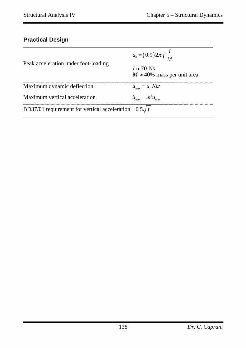
Structural Analysis IV Chapter 5 – Structural Dynamics
Dr. C. Caprani 138
Practical Design
Peak acceleration under foot-loading
00.9 2
Ia f
M
70 NsI 40% mass per unit areaM
Maximum dynamic deflection max stu u K
Maximum vertical acceleration 2
max maxu u
BD37/01 requirement for vertical acceleration 0.5 f

Structural Analysis IV Chapter 5 – Structural Dynamics
Dr. C. Caprani 139
5.6.6 Glossary
Structural dynamics introduces many new terms and concepts so it‟s beneficial to
keep track of them in one place. Fill this out as you progress through the notes.
Symbol Name Units