Embed Size (px)
Citation preview

Structural Analysis IV Chapter 2 – Virtual Work: Compound Structures
Dr. C. Caprani 1
Chapter 2 - Virtual Work: Compound Structures
2.1 Introduction ......................................................................................................... 3
2.1.1 Purpose .......................................................................................................... 3
2.2 Virtual Work Development ................................................................................ 4
2.2.1 The Principle of Virtual Work ....................................................................... 4
2.2.2 Virtual Work for Deflections ......................................................................... 8
2.2.3 Virtual Work for Indeterminate Structures.................................................... 9
2.2.4 Virtual Work for Compound Structures ...................................................... 11
2.3 Basic Examples .................................................................................................. 14
2.3.1 Example 1 .................................................................................................... 14
2.3.2 Example 2 .................................................................................................... 21
2.3.3 Example 3 .................................................................................................... 32
2.3.4 Example 4 .................................................................................................... 40
2.3.5 Problems ...................................................................................................... 48
2.4 Past Exam Questions ......................................................................................... 52
2.4.1 Sample Paper 2007 ...................................................................................... 52
2.4.2 Semester 1 Exam 2007 ................................................................................ 53
2.4.3 Semester 1 Exam 2008 ................................................................................ 54
2.4.4 Semester 1 Exam 2009 ................................................................................ 55
2.4.5 Semester 1 Exam 2010 ................................................................................ 56
2.4.6 Semester 1 Exam 2011 ................................................................................ 57
2.5 Appendix – Trigonometric Integrals ............................................................... 58
2.5.1 Useful Identities ........................................................................................... 58

Structural Analysis IV Chapter 2 – Virtual Work: Compound Structures
Dr. C. Caprani 2
2.5.2 Basic Results ................................................................................................ 59
2.5.3 Common Integrals ....................................................................................... 60
2.6 Appendix – Volume Integrals ........................................................................... 67
Rev. 1

Structural Analysis IV Chapter 2 – Virtual Work: Compound Structures
Dr. C. Caprani 3
2.1 Introduction
2.1.1 Purpose
Previously we only used virtual work to analyse structures whose members primarily
behaved in flexure or in axial forces. Many real structures are comprised of a mixture
of such members. Cable-stay and suspension bridges area good examples: the deck-
level carries load primarily through bending whilst the cable and pylon elements
carry load through axial forces mainly. A simple example is a trussed beam:
Other structures carry load through a mixture of bending, axial force, torsion, etc. Our
knowledge of virtual work to-date is sufficient to analyse such structures.

Structural Analysis IV Chapter 2 – Virtual Work: Compound Structures
Dr. C. Caprani 4
2.2 Virtual Work Development
2.2.1 The Principle of Virtual Work
This states that:
A body is in equilibrium if, and only if, the virtual work of all forces acting on
the body is zero.
In this context, the word ‘virtual’ means ‘having the effect of, but not the actual form
of, what is specified’.
There are two ways to define virtual work, as follows.
1. Virtual Displacement:
Virtual work is the work done by the actual forces acting on the body moving
through a virtual displacement.
2. Virtual Force:
Virtual work is the work done by a virtual force acting on the body moving
through the actual displacements.
Virtual Displacements
A virtual displacement is a displacement that is only imagined to occur:
• virtual displacements must be small enough such that the force directions are
maintained.

Structural Analysis IV Chapter 2 – Virtual Work: Compound Structures
Dr. C. Caprani 5
• virtual displacements within a body must be geometrically compatible with
the original structure. That is, geometrical constraints (i.e. supports) and
member continuity must be maintained.
Virtual Forces
A virtual force is a force imagined to be applied and is then moved through the actual
deformations of the body, thus causing virtual work.
Virtual forces must form an equilibrium set of their own.
Internal and External Virtual Work
When a structures deforms, work is done both by the applied loads moving through a
displacement, as well as by the increase in strain energy in the structure. Thus when
virtual displacements or forces are causing virtual work, we have:
00I E
E I
WW W
W W
δδ δ
δ δ
=− =
=
where
• Virtual work is denoted Wδ and is zero for a body in equilibrium;
• External virtual work is EWδ , and;
• Internal virtual work is IWδ .
And so the external virtual work must equal the internal virtual work. It is in this
form that the Principle of Virtual Work finds most use.

Structural Analysis IV Chapter 2 – Virtual Work: Compound Structures
Dr. C. Caprani 6
Application of Virtual Displacements
For a virtual displacement we have:
0
E I
i i i i
WW W
F y P e
δδ δ
δ δ
==
⋅ = ⋅∑ ∑
In which, for the external virtual work, iF represents an externally applied force (or
moment) and iyδ its virtual displacement. And for the internal virtual work, iP
represents the internal force (or moment) in member i and ieδ its virtual deformation.
The summations reflect the fact that all work done must be accounted for.
Remember in the above, each the displacements must be compatible and the forces
must be in equilibrium, summarized as:
Set of forces in
equilibrium
Set of compatible
displacements

Structural Analysis IV Chapter 2 – Virtual Work: Compound Structures
Dr. C. Caprani 7
Application of Virtual Forces
When virtual forces are applied, we have:
0
E I
i i i i
WW W
y F e P
δδ δ
δ δ
==
⋅ = ⋅∑ ∑
And again note that we have an equilibrium set of forces and a compatible set of
displacements:
In this case the displacements are the real displacements that occur when the structure
is in equilibrium and the virtual forces are any set of arbitrary forces that are in
equilibrium.
Set of compatible
displacements
Set of forces in
equilibrium

Structural Analysis IV Chapter 2 – Virtual Work: Compound Structures
Dr. C. Caprani 8
2.2.2 Virtual Work for Deflections
Deflections in Beams and Frames
For a beam we proceed as:
1. Write the virtual work equation for bending:
0
E I
i i
WW W
y F M
δδ δ
δ θ δ
==
⋅ = ⋅∑
2. Place a unit load, Fδ , at the point at which deflection is required;
3. Find the real bending moment diagram, xM , since the real curvatures are given
by:
xx
x
MEI
θ =
4. Solve for the virtual bending moment diagram (the virtual force equilibrium
set), Mδ , caused by the virtual unit load.
5. Solve the virtual work equation:
0
1L
xx
My M dxEI
δ ⋅ = ⋅ ∫
6. Note that the integration tables can be used for this step.

Structural Analysis IV Chapter 2 – Virtual Work: Compound Structures
Dr. C. Caprani 9
2.2.3 Virtual Work for Indeterminate Structures
General Approach
Using compatibility of displacement, we have:
Final = Primary + Reactant
Next, further break up the reactant structure, using linear superposition:
Reactant = Multiplier × Unit Reactant
We summarize this process as:
0 1M M Mα= +
• M is the force system in the original structure (in this case moments);
• 0M is the primary structure force system;
• 1M is the unit reactant structure force system.
The primary structure can be analysed, as can the unit reactant structure. Thus, the
only unknown is the multiplier, α , for which we use virtual work to calculate.

Structural Analysis IV Chapter 2 – Virtual Work: Compound Structures
Dr. C. Caprani 10
Finding the Multiplier
For beams and frames, we have:
( )210 1
0 0
0L L
ii
i i
MM M dx dxEI EI
δδ α⋅= + ⋅∑ ∑∫ ∫
Thus:
( )
0 1
021
0
Li
i
Li
i
M M dxEI
Mdx
EI
δ
αδ
⋅−=∑∫
∑∫

Structural Analysis IV Chapter 2 – Virtual Work: Compound Structures
Dr. C. Caprani 11
2.2.4 Virtual Work for Compound Structures
Basis
In the general equation for Virtual Work:
i i i iy F e Pδ δ⋅ = ⋅∑ ∑
We note that the summation on the right hand side is over all forms of real
displacement and virtual force combinations. For example, if a member is in
combined bending and axial force, then we must include the work done by both
effects:
( ) ( ) ( )Axial BendingMemberiW e P e P
PL MP M dxEA EI
δ δ δ
δ δ
= ⋅ + ⋅
= ⋅ + ⋅∫
The total Virtual Work done by any member is:
( )Memberiv
PL M T VW P M dx T VEA EI GJ GA
δ δ δ δ δ= ⋅ + ⋅ + ⋅ + ⋅∫
In which Virtual Work done by axial, bending, torsion, and shear, respectively, is
accounted for. However, most members primarily act through only one of these stress
resultants, and so we commonly have only one term per member. A typical example
is when axial deformation of frame (bending) members is neglected; since the area is
large the contribution to virtual work is small.

Structural Analysis IV Chapter 2 – Virtual Work: Compound Structures
Dr. C. Caprani 12
At the level of the structure as a whole, we must account for all such sources of
Virtual Work. For the typical structures we study here, we account for the Virtual
Work done by axial and flexural members separately:
0
E I
i i i i i i
WW W
y F e P M
δδ δ
δ δ θ δ
==
⋅ = ⋅ + ⋅∑ ∑ ∑
In which the first term on the RHS is the internal virtual work done by axial members
and the second term is that done by flexural members.
Again considering only axial and bending members, if a deflection is sought:
0
1
i i i i
Lx
i xi
y F e P M
PL My P M dxEA EI
δ δ θ δ
δ δ
⋅ = ⋅ + ⋅
⋅ = ⋅ + ⋅
∑ ∑
∑ ∑∫
To solve such an indeterminate structure, we have the contributions to Virtual Work:
0 1M M Mα= +
0 1P P Pα= +
for the structure as a whole. Hence we have:

Structural Analysis IV Chapter 2 – Virtual Work: Compound Structures
Dr. C. Caprani 13
( ) ( )
( )
1
0
0 1 0 11
0
210 1 0 11 1
0
0
0 1
0
0
E I
i i i i i i
Lx
i xi
Lx x
i x
i
Lxx x
i ii i
WW W
y F e P M
PL MP M dxEA EI
P P L M MP M dx
EA EI
MP L P L M MP P dxEA EA EI
δδ δ
δ δ θ δ
δ δ
α δ αδ δ
δδ δδ α δ α
==
⋅ = ⋅ + ⋅
⋅ = ⋅ + ⋅
+ ⋅ + = ⋅ + ⋅
⋅= ⋅ + ⋅ ⋅ + + ⋅
∑ ∑ ∑
∑ ∑∫
∑ ∑∫
∑ ∑ ∑∫0
L
dxEI∑∫
Hence the multiplier can be found as:
( ) ( )
0 1 0 1
02 21 1
0
Li i i
i i
Li i i
i i
P P L M M dxEA EI
P L Mdx
EA EI
δ δ
αδ δ
⋅ ⋅ ⋅+= −
+
∑ ∑∫
∑ ∑∫
Note the negative sign!
Though these expressions are cumbersome, the ideas and the algebra are both simple.
Integration of Diagrams
We are often faced with the integration of various diagrams when using virtual work
to calculate the deflections, etc. As such diagrams only have a limited number of
shapes, a table of ‘volume’ integrals is used.

Structural Analysis IV Chapter 2 – Virtual Work: Compound Structures
Dr. C. Caprani 14
2.3 Basic Examples
2.3.1 Example 1
Problem
For the following structure, find:
(a) The force in the cable BC and the bending moment diagram;
(b) The vertical deflection at D.
Take 3 28 10 kNmEI = × and 316 10 kNEA = × .

Structural Analysis IV Chapter 2 – Virtual Work: Compound Structures
Dr. C. Caprani 15
Solution – Part (a)
This is a one degree indeterminate structure and so we must release one redundant.
We could choose many, but the most obvious is the cable, BC. We next analyze the
primary structure for the actual loads, and the unit virtual force placed in lieu of the
redundant:
From the derivation of Virtual Work for indeterminate structures, we have:
( )210 1 0 1
1 1
0 0
0L L
xx xi i
i i
MP L P L M MP P dx dxEA EA EI EI
δδ δδ α δ α ⋅
= ⋅ + ⋅ ⋅ + + ⋅
∑ ∑ ∑ ∑∫ ∫
We evaluate each term separately to simplify the calculations and to minimize
potential calculation error.

Structural Analysis IV Chapter 2 – Virtual Work: Compound Structures
Dr. C. Caprani 16
Term 1:
This term is zero since 0P is zero.
Term 2:
Only member BC contributes to this term and so it is:
1
1 1 2 21ii
P L PEA EA EAδ δ ⋅
⋅ = ⋅ =
∑
Term 3:
Here we must integrate the bending moment diagrams. We use the volume integral
for the portion AD of both diagrams. Thus we multiply a triangle by a trapezoid:
( ) ( )( )( )
0 1
0
1 1 40 2 2 4 26
400 3
Lx xM M dxEI EI
EI
δ⋅ = − + −
= −
∑∫
Term 4:
Here we multiply the virtual BMD by itself so it is a triangle by a triangle:
( ) ( )( )( )
21
0
1 1 64 34 4 43
LxM
dxEI EI EI
δ = − − = ∑∫
With all terms evaluated the Virtual Work equation becomes:
2 400 3 64 30 0EA EI EI
α α= + ⋅ − + ⋅

Structural Analysis IV Chapter 2 – Virtual Work: Compound Structures
Dr. C. Caprani 17
Which gives:
400 3400
2 64 3 6 64EI
EIEA EI EA
α = =+ +
Given that 3 38 10 16 10 0.5EI EA = × × = , we have:
( )
400 5.976 0.5 64
α = =+
Thus there is a tension (positive answer) in the cable of 5.97 kN, giving the BMD as:
Note that this comes from:
( )( )( )( )
0
0
40 5.97 4 16.1 kN
0 5.97 2 11.9 kNA
D
M M M
M M M
α δ
α δ
= + ⋅ = + − =
= + ⋅ = + − = −

Structural Analysis IV Chapter 2 – Virtual Work: Compound Structures
Dr. C. Caprani 18
Solution – Part (b)
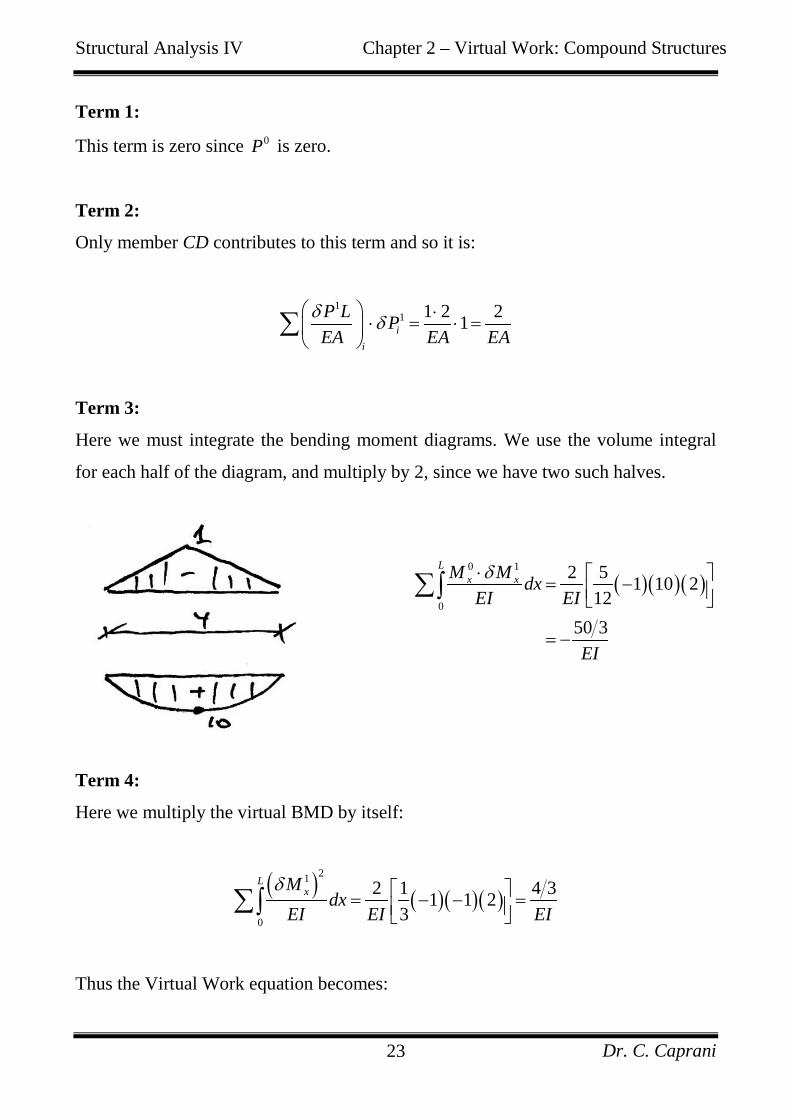
Recalling that the only requirement on applying virtual forces to calculate real
displacements is that an equilibrium system results, we can apply a vertical unit force
at D to the primary structure only:
The Virtual Work equation useful for deflection is:
0
1
i i i i
Lx
Dy i xi
y F e P M
PL MP M dxEA EI
δ δ θ δ
δ δ δ
⋅ = ⋅ + ⋅
⋅ = ⋅ + ⋅
∑ ∑
∑ ∑∫
Since 0Pδ = , we need only calculate the term involving the Virtual Work done by
the beam bending. This involves the volume integral of the two diagrams:

Structural Analysis IV Chapter 2 – Virtual Work: Compound Structures
Dr. C. Caprani 19
Note that only the portion AD will count as there is no virtual moment on DB. Thus
we have:
However, this shape is not easy to work with, given the table to hand. Therefore we
recall that the real BMD came about as the superposition of two BMD shapes that are
easier to work with, and so we have:
A further benefit of this approach is that an equation of deflection in terms of the
multiplier α is got. This could then be used to determine α for a particular design
requirement, and in turn this could inform the choice of EI EA ratio. Thus:
( )( )( ) ( ) ( )( )( )
0
1 1 12 40 2 2 2 2 4 23 6
160 203
Lx
Dy xM M dxEI
EI
EI
δ δ
α
α
= ⋅
= + ⋅ − + − −
=
∑∫

Structural Analysis IV Chapter 2 – Virtual Work: Compound Structures
Dr. C. Caprani 20
Given 5.97α = , we then have:
( ) 33
160 20 5.97 13.9 13.9 10 1.7 mm3 8 10Dy EI EI
δ−
= = = × =×
The positive answer indicates that the deflection is in the direction of the applied
virtual vertical force and so is downwards as expected.
We can also easily work out the deflection at B, since it is the same as the elongation
of the cable:
( )( ) 33
5.97 210 0.75 mm
16 10ByPLEA
δ = = × =×
Draw the deflected shape of the structure.

Structural Analysis IV Chapter 2 – Virtual Work: Compound Structures
Dr. C. Caprani 21
2.3.2 Example 2
Problem
For the following structure, find:
(a) The force in the cable CD and the bending moment diagram;
(b) Determine the optimum EA of the cable for maximum efficiency of the beam.
Take 3 28 10 kNmEI = × and 348 10 kNEA = × .

Structural Analysis IV Chapter 2 – Virtual Work: Compound Structures
Dr. C. Caprani 22
Solution – Part (a)
Choose the cable CD as the redundant to give:
The equation of Virtual Work relevant is:
( )210 1 0 1
1 1
0 0
0L L
xx xi i
i i
MP L P L M MP P dx dxEA EA EI EI
δδ δδ α δ α ⋅
= ⋅ + ⋅ ⋅ + + ⋅
∑ ∑ ∑ ∑∫ ∫
We evaluate each term separately:
Structural Analysis IV Chapter 2 – Virtual Work: Compound Structures
Dr. C. Caprani 23
Term 1:
This term is zero since 0P is zero.
Term 2:
Only member CD contributes to this term and so it is:
1
1 1 2 21ii
P L PEA EA EAδ δ ⋅
⋅ = ⋅ =
∑
Term 3:
Here we must integrate the bending moment diagrams. We use the volume integral
for each half of the diagram, and multiply by 2, since we have two such halves.
( )( )( )
0 1
0
2 5 1 10 212
50 3
Lx xM M dxEI EI
EI
δ⋅ = −
= −
∑∫
Term 4:
Here we multiply the virtual BMD by itself:
( ) ( )( )( )
21
0
2 1 4 31 1 23
LxM
dxEI EI EI
δ = − − = ∑∫
Thus the Virtual Work equation becomes:

Structural Analysis IV Chapter 2 – Virtual Work: Compound Structures
Dr. C. Caprani 24
2 50 3 4 30 0EA EI EI
α α= + ⋅ − + ⋅
Which gives:
50 350
2 4 3 6 4EI
EIEA EI EA
α = =+ +
Given that 3 38 10 48 10 0.167EI EA = × × = , we have:
( )
50 106 0.167 4
α = =+
Thus there is a tension (positive answer) in the cable of 10 kN, giving:

Structural Analysis IV Chapter 2 – Virtual Work: Compound Structures
Dr. C. Caprani 25
As designers, we want to control the flow of forces. In this example we can see that
by changing the ratio EI EA we can control the force in the cable, and the resulting
bending moments. We can plot the cable force and maximum sagging bending
moment against the stiffness ratio to see the behaviour for different relative
stiffnesses:
0
2
4
6
8
10
12
14
0.0001 0.001 0.01 0.1 1 10 100 1000 10000
Ratio EI/EA
Cable Tension (kN)Sagging Moment (kNm)

Structural Analysis IV Chapter 2 – Virtual Work: Compound Structures
Dr. C. Caprani 26
Solution – Part (b)
Efficiency of the beam means that the moments are resisted by the smallest possible
beam. Thus the largest moment anywhere in the beam must be made as small as
possible. Therefore the hogging and sagging moments should be equal:
We know that the largest hogging moment will occur at 2L . However, we do not
know where the largest sagging moment will occur. Lastly, we will consider sagging
moments positive and hogging moments negative. Consider the portion of the net
bending moment diagram, ( )M x , from 0 to 2L :
The equations of these bending moments are:

Structural Analysis IV Chapter 2 – Virtual Work: Compound Structures
Dr. C. Caprani 27
( )2P
PM x x= −
( ) 2
2 2W
w wLM x x x= − +
Thus:
( ) ( ) ( )
2
2 2 2
W PM x M x M xwL w Px x x
= +
= − −
The moment at 2L is:
( )2
2 2
2
22 2 2 2 2 2
4 8 4
8 4
wL L w L P LM L
wL wL PL
wL PL
= − −
= − −
= −
Which is as we expected. The maximum sagging moment between 0 and 2L is
found at:

Structural Analysis IV Chapter 2 – Virtual Work: Compound Structures
Dr. C. Caprani 28
( )
max
max
0
02 2
2 2
dM xdx
wL Pwx
L Pxw
=
− − =
= −
Thus the maximum sagging moment has a value:
( )2
max
2 2 2 2
2 2
2 2 2 2 2 2 2 2 22
4 4 2 4 4 4 4 4
8 4 8
wL L P w L P P L PM xw w w
wL PL w L PL P PL Pw w w
wL PL Pw
= − − − − −
= − − − + − +
= − +
Since we have assigned a sign convention, the sum of the hogging and sagging
moments should be zero, if we are to achieve the optimum BMD. Thus:
( ) ( )max
2 2 2
2 2
22
2 0
08 4 8 8 4
04 2 8
1 08 2 4
M x M L
wL PL P wL PLw
wL PL Pw
L wLP Pw
+ =
− + + − =
− + =
+ − + =
This is a quadratic equation in P and so we solve for P using the usual method:

Structural Analysis IV Chapter 2 – Virtual Work: Compound Structures
Dr. C. Caprani 29
( )
2 2
82 4 82 2 2 8
82 2
L L Lw L LP
wwL
± − = = ±
= ±
Since the load in the cable must be less than the total amount of load in the beam, that
is, P wL< , we have:
( )2 2 0.586P wL wL= − =
With this value for P we can determine the hogging and sagging moments:
( )( )2
2
2
2 22
8 42 2 3
8
0.0214
wL LwLM L
wL
wL
−= −
−=
= −
And:
( )
( )
2 2
max
2
2
2
2
8 4 8
2 22 2 38 8
3 2 28
0.0214
wL PL PM xw
wLwL
w
wL
wL
= − +
− − = + −
=
= +

Structural Analysis IV Chapter 2 – Virtual Work: Compound Structures
Dr. C. Caprani 30
Lastly, the location of the maximum sagging moment is given by:
( )
( )
max 2 22 2
2 2
2 120.207
L Pxw
wLLw
L
L
= −
−= −
= −
=
For our particular problem, 5 kN/mw = , 4 mL = , giving:
( )0.586 5 4 11.72 kNP = × =
( ) ( )2max 0.0214 5 4 1.71 kNmM x = × =
Thus, as we expected, 10 kNP > , the value obtained from Part (a) of the problem.
Now since, we know P we now also know the required value of the multiplier, α .
Hence, we write the virtual work equations again, but this time keeping Term 2 in
terms of L, since that is what we wish to solve for:
50 11.726 4
1 50 4 0.0446 11.72
EIEA
EIEA
α = =+
∴ = − =
Giving 3 38 10 0.044 180.3 10 kNEA = × = × . This is 3.75 times the original cable area
– a lot of extra material just to change the cable force by 17%. However, there is a

Structural Analysis IV Chapter 2 – Virtual Work: Compound Structures
Dr. C. Caprani 31
large saving by reducing the overall moment in the beam from 10 kNm (simply-
supported) or 2.5 kNm (two-span beam) to 1.71 kNm.

Structural Analysis IV Chapter 2 – Virtual Work: Compound Structures
Dr. C. Caprani 32
2.3.3 Example 3
Problem
For the following structure:
1. Determine the tension in the cable AB;
2. Draw the bending moment diagram;
3. Determine the vertical deflection at D with and without the cable AB.
Take 3 2120 10 kNmEI = × and 360 10 kNEA = × .

Structural Analysis IV Chapter 2 – Virtual Work: Compound Structures
Dr. C. Caprani 33
Solution
As is usual, we choose the cable to be the redundant member and split the frame up
as follows:
Primary Structure Redundant Structure
We must examine the BMDs carefully, and identify expressions for the moments
around the arch. However, since we will be using virtual work and integrating one
diagram against another, we immediately see that we are only interested in the
portion of the structure CB. Further, we will use the anti-clockwise angle from
vertical as the basis for our integration.
Primary BMD
Drawing the BMD and identify the relevant distances:

Structural Analysis IV Chapter 2 – Virtual Work: Compound Structures
Dr. C. Caprani 34
Hence the expression for 0M is:
( ) ( )0 20 10 2sin 20 1 sinMθ θ θ= + = +
Reactant BMD
This calculation is slightly easier:

Structural Analysis IV Chapter 2 – Virtual Work: Compound Structures
Dr. C. Caprani 35
( ) ( )1 1 2 2cos 2 1 cosMθ θ θ= ⋅ − = −
Virtual Work Equation
As before, we have the equation:
( )210 1 0 11 1
0 0
0L L
xx xi i
i i
MP L P L M MP P dx dxEA EA EI EI
δδ δδ α δ α ⋅
= ⋅ + ⋅ ⋅ + + ⋅
∑ ∑ ∑ ∑∫ ∫
Term 1 is zero since there are no axial forces in the primary structure. We take each
other term in turn.
Term 2
Since only member AB has axial force:
( )21 2 2Term 2EA EA
= =
Term 3

Structural Analysis IV Chapter 2 – Virtual Work: Compound Structures
Dr. C. Caprani 36
Since we want to integrate around the member – an integrand ds - but only have the
moment expressed according to θ , we must change the integration limits by
substituting:
2ds R d dθ θ= ⋅ =
Hence:
( ) ( )
( )( )
( )
20 1
0 0
2
0
2
0
1 2 1 cos 20 1 sin 2
80 1 cos 1 sin
80 1 sin cos cos sin
Lx xM M dx dEI EI
dEI
dEI
π
π
π
δ θ θ θ
θ θ θ
θ θ θ θ θ
⋅= − − +
= − + +
= − − + +
∑∫ ∫
∫
∫
To integrate this expression we refer to the appendix of integrals to get each of the
terms, which then give:
( )
20 1
00
80 1cos sin cos24
80 1 10 1 1 0 1 02 4 4
80 1 11 12 4 4
80 12
Lx xM M dxEI EI
EI
EI
EI
πδ θ θ θ θ
π
π
π
⋅ = − + + −
= − + + − − − − + + − = − + + − + − =
∑∫
Term 4

Structural Analysis IV Chapter 2 – Virtual Work: Compound Structures
Dr. C. Caprani 37
Proceeding similarly to Term 3, we have:
( ) ( ) ( )
( )
21 2
0 0
22
0
1 2 1 cos 2 1 cos 2
8 1 2cos cos
LxM
dx dEI EI
dEI
π
π
δθ θ θ
θ θ θ
= − −
= − +
∑∫ ∫
∫
Again we refer to the integrals appendix, and so for Term 4 we then have:
( ) ( )
[ ]
21 22
0 0
2
0
8 1 2cos cos
8 12sin sin 22 4
8 12 0 0 0 02 4 4
8 3 74
LxM
dx dEI EI
EI
EI
EI
π
π
δθ θ θ
θθ θ θ
π π
π
= − +
= − + +
= − + + − − + + − =
∑∫ ∫
Solution
Substituting the calculated values into the virtual work equation gives:
2 80 1 8 3 70 02 4EA EI EIπ πα α− − = + ⋅ + + ⋅
And so:

Structural Analysis IV Chapter 2 – Virtual Work: Compound Structures
Dr. C. Caprani 38
80 12
2 8 3 74
EI
EA EI
π
απ
− − =
− +
Simplifying:
20 20
3 7 EIEA
παπ
−=
− +
In this problem, 2EI EA = and so:
20 20 9.68 kN3 5παπ−
= =−
We can examine the effect of different ratios of EI EA on the structure from our
algebraic solution for α . We show this, as well as a point representing the solution
for this particular EI EA ratio on the following graph:
0
2
4
6
8
10
12
14
16
18
20
0.0001 0.001 0.01 0.1 1 10 100 1000 10000
Ratio EI/EA
α F
acto
r

Structural Analysis IV Chapter 2 – Virtual Work: Compound Structures
Dr. C. Caprani 39
As can be seen, by choosing a stiffer frame member (increasing EI) or by reducing
the area of the cable, we can reduce the force in the cable (which is just 1 α⋅ ).
However this will have the effect of increasing the moment at A, for example:
Deflections and shear would also be affected.
Draw the final BMD and determine the deflection at D.
0
5
10
15
20
25
30
35
40
45
0.0001 0.001 0.01 0.1 1 10 100 1000 10000
Ratio EI/EA
Ben
ding
Mom
ent a
t A (k
Nm
)

Structural Analysis IV Chapter 2 – Virtual Work: Compound Structures
Dr. C. Caprani 40
2.3.4 Example 4
Problem
For the following structure:
1. draw the bending moment diagram;
2. Find the vertical deflection at E.
Take 3 2120 10 kNmEI = × and 360 10 kNEA = × .

Structural Analysis IV Chapter 2 – Virtual Work: Compound Structures
Dr. C. Caprani 41
Solution
To begin we choose the cable BF as the obvious redundant, yielding:
Virtual Work Equation
The Virtual Work equation is as before:
( )210 1 0 11 1
0 0
0L L
xx xi i
i i
MP L P L M MP P dx dxEA EA EI EI
δδ δδ α δ α ⋅
= ⋅ + ⋅ ⋅ + + ⋅
∑ ∑ ∑ ∑∫ ∫
Term 1 is zero since there are no axial forces in the primary structure. As we have
done previously, we take each other term in turn.
Term 2

Structural Analysis IV Chapter 2 – Virtual Work: Compound Structures
Dr. C. Caprani 42
Though member AB has axial force, it is primarily a flexural member and so we only
take account of the axial force in the cable BF:
1
1 1 2 2 2 21ii
P L PEA EA EAδ δ
⋅ ⋅ = ⋅ =
∑
Term 3
Since only the portion AB has moment on both diagrams, it is the only section that
requires integration here. Thus:
( )( )( )0 1
0
1 1 220 2200 2 22
Lx xM M dxEI EI EIδ⋅ − = − =
∑∫
Term 3
Similar to Term 3, we have:
( ) ( )( )( )
21
0
1 1 4 32 2 23
LxM
dxEI EI EI
δ = − − = ∑∫
Solution
Substituting the calculated values into the virtual work equation gives:
2 2 220 2 4 30 0EA EI EI
α α= + ⋅ − + ⋅
Thus:

Structural Analysis IV Chapter 2 – Virtual Work: Compound Structures
Dr. C. Caprani 43
220 22 2 4 3
EI
EA EI
α =+
And so:
220 242 23
EIEA
α =+
Since:
3
3
120 10 260 10
EIEA
×= =
×
We have:
( )220 2 40.4642 2 2
3
α = = ++
Thus the force in the cable BF is 40.46 kN tension, as assumed.
The bending moment diagram follows from superposition of the two previous
diagrams:

Structural Analysis IV Chapter 2 – Virtual Work: Compound Structures
Dr. C. Caprani 44
To find the vertical deflection at E, we must apply a unit vertical load at E. We will
apply a downwards load since we think the deflection is downwards. Therefore we
should get a positive result to confirm our expectation.
We need not apply the unit vertical force to the whole structure, as it is sufficient to
apply it to a statically determinate sub-structure. Thus we apply the force as follows:
For the deflection, we have the following equation:
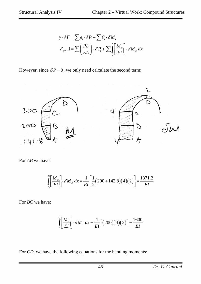
Structural Analysis IV Chapter 2 – Virtual Work: Compound Structures
Dr. C. Caprani 45
0
1
i i i i
Lx
Ey i xi
y F e P M
PL MP M dxEA EI
δ δ θ δ
δ δ δ
⋅ = ⋅ + ⋅
⋅ = ⋅ + ⋅
∑ ∑
∑ ∑∫
However, since 0Pδ = , we only need calculate the second term:
For AB we have:
( )( )( )1 1 1371.2200 142.8 4 22
Bx
xA
M M dxEI EI EI
δ ⋅ = + = ∫
For BC we have:
( )( )( )1 1600200 4 2C
xx
B
M M dxEI EI EI
δ ⋅ = = ∫
For CD, we have the following equations for the bending moments:

Structural Analysis IV Chapter 2 – Virtual Work: Compound Structures
Dr. C. Caprani 46
( ) ( )( )100 2sin200sin
M θ θθ
=
= ( ) ( )( )2 1 2sin
2 2sinMδ θ θ
θ= +
= +
Also note that we want to integrate around the member – an integrand ds - but only
have the moment expressed according to θ , we must change the integration limits by
substituting:
2ds R d dθ θ= ⋅ =
Thus we have:
( )( )
( )
2
0
22
0
2 22
0 0
1 200sin 2 2sin 2
800 sin sin
800 sin sin
Dx
xC
M M dx dEI EI
dEI
d dEI
π
π
π π
δ θ θ θ
θ θ θ
θ θ θ θ
⋅ = + ⋅
= +
= +
∫ ∫
∫
∫ ∫
Taking each term in turn:

Structural Analysis IV Chapter 2 – Virtual Work: Compound Structures
Dr. C. Caprani 47
[ ] ( )2
2
00
sin cos 0 1 1dπ
πθ θ θ= − = − − − = +∫
( ) ( )22
2 22 2
00
1 1 1 1sin sin 1 0 02 4 4 4 4 4
dππ θ π πθ θ θ − = − = − − − = ∫
Thus:
800 1 200 60014
Dx
xC
M M dxEI EI EI
π πδ − + ⋅ = + = ∫
Thus:
1371.2 1600 200 600 4200Ey EI EI EI EI
πδ += + + = +
Thus we get a downwards deflection as expected. Also, since 3 2120 10 kNmEI = × ,
we have:
3
4200 35 mm120 10Eyδ = = ↓
×

Structural Analysis IV Chapter 2 – Virtual Work: Compound Structures
Dr. C. Caprani 48
2.3.5 Problems
Problem 1
For the following structure, find the BMD and the vertical deflection at D. Take 3 28 10 kNmEI = × and 316 10 kNEA = × .
(Ans. 7.8α = for BC, 1.93 mmByδ = ↓ )
Problem 2
For the following structure, find the BMD and the vertical deflection at C. Take 3 28 10 kNmEI = × and 316 10 kNEA = × .
(Ans. 25.7α = for BD, 25 mmCvδ = ↓ )

Structural Analysis IV Chapter 2 – Virtual Work: Compound Structures
Dr. C. Caprani 49
Problem 3
For the following structure, find the BMD and the horizontal deflection at C. Take 3 28 10 kNmEI = × and 316 10 kNEA = × .
(Ans. 47.8α = for BD, 44.8 mmCxδ = → )
Problem 4
For the following structure, find the BMD and the vertical deflection at B. Take P =
20 kN, 3 28 10 kNmEI = × and 316 10 kNEA = × .

Structural Analysis IV Chapter 2 – Virtual Work: Compound Structures
Dr. C. Caprani 50
(Ans. 14.8α = for CD, 14.7 mmByδ = ↓ )
Problem 5
For the following structure, find the BMD and the vertical deflection at C. Take 3 250 10 kNmEI = × and 320 10 kNEA = × .
(Ans. 100.5α = for BC, 55.6 mmCyδ = ↓)
Problem 6
Analyze the following structure and determine the BMD and the vertical deflection at
D. For ABCD, take 210 kN/mmE = , 4 212 10 mmA = × and 8 436 10 mmI = × , and for
AEBFC take 2200 kN/mmE = and 3 22 10 mmA = × .
(Ans. 109.3α = for BF, 54.4 mmCyδ = ↓)

Structural Analysis IV Chapter 2 – Virtual Work: Compound Structures
Dr. C. Caprani 51
Problem 7
Analyze the following structure. For all members, take 210 kN/mmE = , for ABC, 4 26 10 mmA = × and 7 4125 10 mmI = × ; for all other members 21000 mmA = .
(Ans. 72.5α = for DE)

Structural Analysis IV Chapter 2 – Virtual Work: Compound Structures
Dr. C. Caprani 52
2.4 Past Exam Questions
2.4.1 Sample Paper 2007
3. For the rigidly jointed frame shown in Fig. Q3, using Virtual Work:
(i) Determine the bending moment moments due to the loads as shown; (15 marks)
(ii) Draw the bending moment diagram, showing all important values;
(4 marks)
(iii) Determine the reactions at A and E; (3 marks)
(iv) Draw the deflected shape of the frame.
(3 marks) Neglect axial effects in the flexural members. Take the following values: I for the frame = 150×106 mm4; Area of the stay EB = 100 mm2; Take E = 200 kN/mm2 for all members.
FIG. Q3

Structural Analysis IV Chapter 2 – Virtual Work: Compound Structures
Dr. C. Caprani 53
2.4.2 Semester 1 Exam 2007
3. For the rigidly jointed frame shown in Fig. Q3, using Virtual Work:
(i) Determine the bending moment moments due to the loads as shown; (15 marks)
(ii) Draw the bending moment diagram, showing all important values;
(4 marks)
(iii) Determine the reactions at A and E; (3 marks)
(iv) Draw the deflected shape of the frame.
(3 marks) Neglect axial effects in the flexural members. Take the following values: I for the frame = 150×106 mm4; Area of the stay EF = 200 mm2; Take E = 200 kN/mm2 for all members.
Ans. 35.0α = .
FIG. Q3

Structural Analysis IV Chapter 2 – Virtual Work: Compound Structures
Dr. C. Caprani 54
2.4.3 Semester 1 Exam 2008
QUESTION 3
For the frame shown in Fig. Q3, using Virtual Work:
(i) Determine the force in the tie; (ii) Draw the bending moment diagram, showing all important values; (iii) Determine the deflection at C; (iv) Determine an area of the tie such that the bending moments in the beam are minimized; (v) For this new area of tie, determine the deflection at C; (vi) Draw the deflected shape of the structure.
(25 marks)
Note:
Neglect axial effects in the flexural members and take the following values:
• For the frame, 6 4600 10 mmI = × ; • For the tie, 2300 mmA = ; • For all members, 2200 kN/mmE = .
Ans. 21.24α = ; 4.1 mmCyδ = ↓ ; 22160 mmA = ; 2.0 mmCyδ = ↓
FIG. Q3

Structural Analysis IV Chapter 2 – Virtual Work: Compound Structures
Dr. C. Caprani 55
2.4.4 Semester 1 Exam 2009
QUESTION 3
For the frame shown in Fig. Q3, using Virtual Work:
(i) Determine the axial forces in the members; (ii) Draw the bending moment diagram, showing all important values; (iii) Determine the reactions; (iv) Determine the vertical deflection at D; (v) Draw the deflected shape of the structure.
(25 marks)
Note:
Neglect axial effects in the flexural members and take the following values:
• For the beam ABCD, 6 4600 10 mmI = × ; • For members BF and CE, 2300 mmA = ; • For all members, 2200 kN/mmE = .
Ans. 113.7α = (for CE); 55 mmDyδ = ↓
FIG. Q3

Structural Analysis IV Chapter 2 – Virtual Work: Compound Structures
Dr. C. Caprani 56
2.4.5 Semester 1 Exam 2010 QUESTION 3 For the frame shown in Fig. Q3, using Virtual Work:
(i) Draw the bending moment diagram, showing all important values;
(ii) Determine the horizontal displacement at C;
(iii) Determine the vertical deflection at C;
(iv) Draw the deflected shape of the structure.
(25 marks) Note: Neglect axial effects in the flexural members and take the following values:
• For the beam ABC, 3 25 10 kNmEI = × ; • For member BD, 2200 kN/mmE = and 2200 mmA = ; • The following integral results may assist in your solution:
sin cosdθ θ θ= −∫ 1cos sin cos 24
dθ θ θ θ= −∫ 2 1sin sin 22 4
d θθ θ θ= −∫
Ans. 37.1α = (for BD); 104 mmCxδ = ← 83 mmCyδ = ↓
FIG. Q3

Structural Analysis IV Chapter 2 – Virtual Work: Compound Structures
Dr. C. Caprani 57
2.4.6 Semester 1 Exam 2011 QUESTION 3 For the frame shown in Fig. Q3, using Virtual Work: (i) Draw the bending moment diagram, showing all important values; (ii) Draw the axial force diagram; (iii) Determine the vertical deflection at D; (iv) Draw the deflected shape of the structure.
(25 marks) Note: Neglect axial effects in the flexural members and take the following values:
• For the member ABCD, 3 25 10 kNmEI = × ; • For members BF and CE, 2200 kN/mmE = and 2200 mmA = ; • The following integral result may assist in your solution:
2 1sin sin 2
2 4d θθ θ θ= −∫
Ans. 48.63α = (for BF); 108.4 mmDyδ = ↓
FIG. Q3

Structural Analysis IV Chapter 2 – Virtual Work: Compound Structures
Dr. C. Caprani 58
2.5 Appendix – Trigonometric Integrals
2.5.1 Useful Identities
In the following derivations, use is made of the trigonometric identities:
1cos sin sin 22
θ θ θ= (1)
( )2 1cos 1 cos22
θ θ= + (2)
( )2 1sin 1 cos22
θ θ= − (3)
Integration by parts is also used:
u dx ux x du C= − +∫ ∫ (4)

Structural Analysis IV Chapter 2 – Virtual Work: Compound Structures
Dr. C. Caprani 59
2.5.2 Basic Results
Neglecting the constant of integration, some useful results are:
cos sindθ θ θ=∫ (5)
sin cosdθ θ θ= −∫ (6)
1sin cosa d aa
θ θ θ= −∫ (7)
1cos sina d aa
θ θ θ=∫ (8)

Structural Analysis IV Chapter 2 – Virtual Work: Compound Structures
Dr. C. Caprani 60
2.5.3 Common Integrals
The more involved integrals commonly appearing in structural analysis problems are:
cos sin dθ θ θ∫
Using identity (1) gives:
1cos sin sin 22
d dθ θ θ θ θ=∫ ∫
Next using (7), we have:
1 1 1sin 2 cos22 2 2
1 cos24
dθ θ θ
θ
= −
= −
∫
And so:
1cos sin cos24
dθ θ θ θ= −∫ (9)

Structural Analysis IV Chapter 2 – Virtual Work: Compound Structures
Dr. C. Caprani 61
2cos dθ θ∫
Using (2), we have:
( )2 1cos 1 cos2
21 1 cos22
d d
d d
θ θ θ θ
θ θ θ
= +
= +
∫ ∫
∫ ∫
Next using (8):
1 1 11 cos2 sin 22 2 2
1 sin 22 4
d dθ θ θ θ θ
θ θ
+ = +
= +
∫ ∫
And so:
2 1cos sin 22 4
d θθ θ θ= +∫ (10)

Structural Analysis IV Chapter 2 – Virtual Work: Compound Structures
Dr. C. Caprani 62
2sin dθ θ∫
Using (3), we have:
( )2 1sin 1 cos2
21 1 cos22
d d
d d
θ θ θ θ
θ θ θ
= −
= −
∫ ∫
∫ ∫
Next using (8):
1 1 11 cos2 sin 22 2 2
1 sin 22 4
d dθ θ θ θ θ
θ θ
− = −
= −
∫ ∫
And so:
2 1sin sin 22 4
d θθ θ θ= −∫ (11)

Structural Analysis IV Chapter 2 – Virtual Work: Compound Structures
Dr. C. Caprani 63
cos dθ θ θ∫
Using integration by parts write:
cos d u dxθ θ θ =∫ ∫
Where:
cosu dx dθ θ θ= =
To give:
du dθ=
And
cos
sin
dx d
x
θ θ
θ
=
=∫ ∫
Which uses (5). Thus, from (4), we have:
cos sin sin
u dx ux x du
d dθ θ θ θ θ θ θ
= −
= −∫ ∫
∫ ∫
And so, using (6) we have:
cos sin cosdθ θ θ θ θ θ= +∫ (12)

Structural Analysis IV Chapter 2 – Virtual Work: Compound Structures
Dr. C. Caprani 64
sin dθ θ θ∫
Using integration by parts write:
sin d u dxθ θ θ =∫ ∫
Where:
sinu dx dθ θ θ= =
To give:
du dθ=
And
sin
cos
dx d
x
θ θ
θ
=
= −∫ ∫
Which uses (6). Thus, from (4), we have:
( ) ( )sin cos cos
u dx ux x du
d dθ θ θ θ θ θ θ
= −
= − − −∫ ∫
∫ ∫
And so, using (5) we have:
sin cos sindθ θ θ θ θ θ= − +∫ (13)

Structural Analysis IV Chapter 2 – Virtual Work: Compound Structures
Dr. C. Caprani 65
( )cos A dθ θ−∫
Using integration by substitution, we write u A θ= − to give:
1duddu dθ
θ
= −
= −
Thus:
( ) ( )cos cosA d u duθ θ− = −∫ ∫
And since, using (5):
cos sinu du u− = −∫
We have:
( ) ( )cos sinA d Aθ θ θ− = − −∫ (14)

Structural Analysis IV Chapter 2 – Virtual Work: Compound Structures
Dr. C. Caprani 66
( )sin A dθ θ−∫
Using integration by substitution, we write u A θ= − to give:
1duddu dθ
θ
= −
= −
Thus:
( ) ( )sin sinA d u duθ θ− = −∫ ∫
And since, using (6):
( )sin cosu du u− = − −∫
We have:
( ) ( )sin cosA d Aθ θ θ− = −∫ (15)

Structural Analysis IV Chapter 2 – Virtual Work: Compound Structures
Dr. C. Caprani 67
2.6 Appendix – Volume Integrals
13
jkl 16
jkl ( )1 21 26
j j kl+ 12
jkl
16
jkl 13
jkl ( )1 21 26
j j kl+ 12
jkl
( )1 2
1 26
j k k l+ ( )1 21 26
j k k l+ ( )
( )
1 1 2
2 1 2
1 26
2
j k k
j k k l
+ +
+
( )1 212
j k k l+
12
jkl 12
jkl ( )1 212
j j kl+ jkl
( )1
6jk l a+ ( )1
6jk l b+
( )
( )
1
2
16
j l b
j l a k
+ +
+
12
jkl
512
jkl 14
jkl ( )1 21 3 5
12j j kl+ 2
3jkl
14
jkl 512
jkl ( )1 21 5 3
12j j kl+ 2
3jkl
14
jkl 112
jkl ( )1 21 3
12j j kl+ 1
3jkl
112
jkl 14
jkl ( )1 21 3
12j j kl+ 1
3jkl
13
jkl 13
jkl ( )1 213
j j kl+ 23
jkl
1 2
1 2