Embed Size (px)
Citation preview

1
The Islamic University of Gaza
Faculty of Engineering
Civil Engineering Department
Hydraulics - ECIV 3322
Water Distribution Systems
Chapter 4

2
Introduction To deliver water to individual consumers with appropriate
quality, quantity, and pressure in a community setting requires
an extensive system of:
Pipes.
Storage reservoirs.
Pumps.
Other related accessories.
Distribution system: is used to describe collectively the
facilities used to supply water from its source to the point of
usage .
3
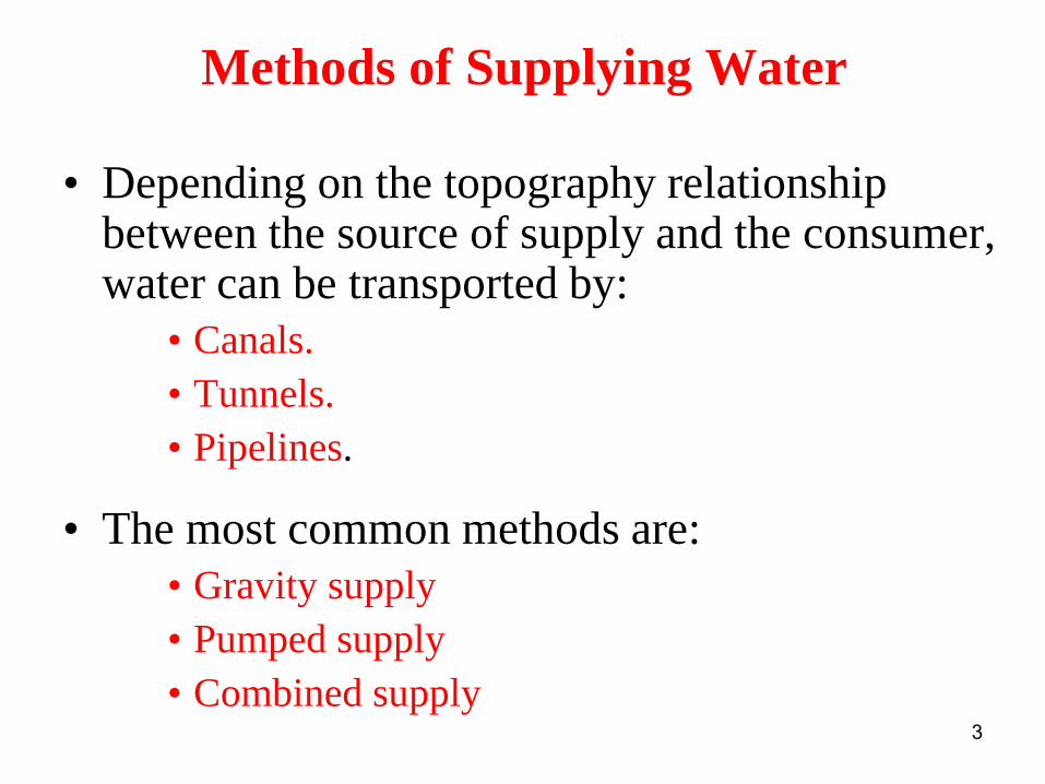
Methods of Supplying Water
• Depending on the topography relationship between the source of supply and the consumer, water can be transported by:
• Canals.
• Tunnels.
• Pipelines.
• The most common methods are:
• Gravity supply
• Pumped supply
• Combined supply

4
Gravity Supply
• The source of supply is at a sufficient elevation
above the distribution area (consumers). so that the desired pressure can be maintained
Source
(Reservoir) (Consumers)
Gravity-Supply System
HGL or EGL

5
Advantages of Gravity supply
• No energy costs.
• Simple operation (fewer mechanical parts,
independence of power supply, ….)
• Low maintenance costs.
• No sudden pressure changes
Source
HGL or EGL

6
Pumped Supply Used whenever:
• The source of water is lower than the area to which we need to
distribute water to (consumers)
• The source cannot maintain minimum pressure required.
pumps are used to develop the necessary head (pressure) to
distribute water to the consumer and storage reservoirs.
Source
(River/Reservoir)
(Consumers)
Pumped-Supply System
HGL or EGL

7
Source
(River/Reservoir)
(Consumers)
HGL or EGL
Disadvantages of pumped supply
Complicated operation and maintenance.
Dependent on reliable power supply.
Precautions have to be taken in order to enable permanent supply:
• Stock with spare parts
• Alternative source of power supply ….

8
Combined Supply
(pumped-storage supply)
• Both pumps and storage reservoirs are used.
• This system is usually used in the following cases:
1) When two sources of water are used to supply water:
Source (1)
Source (2)
City
Gravity
Pumping
HGL
HGL
Pumping station

9
Combined Supply (Continue) 2) In the pumped system sometimes a storage (elevated)
tank is connected to the system.
Elevated
tank
Source
Pipeline
High
consumption
Pumping station
• When the water consumption is low, the residual water is
pumped to the tank.
• When the consumption is high the water flows back to
the consumer area by gravity.
Low consumption
City

10
Combined Supply (Continue) 3) When the source is lower than the consumer area
Reservoir
Source
Pumping
Pumping Station
• A tank is constructed above the highest point in the area,
• Then the water is pumped from the source to the storage
tank (reservoir).
• And the hence the water is distributed from the reservoir
by gravity.
Gravity
City
HGL
HGL
11
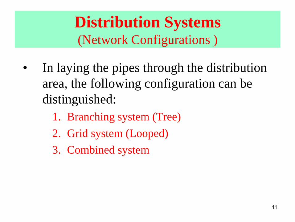
Distribution Systems (Network Configurations )
• In laying the pipes through the distribution
area, the following configuration can be
distinguished:
1. Branching system (Tree)
2. Grid system (Looped)
3. Combined system

12
Branching System (tree system)
Branching System
Source
Submain
Main
pipe
Dead End
Advantages:
• Simple to design and build.
• Less expensive than other systems.

13
• The large number of dead ends which results in sedimentation
and bacterial growths.
• When repairs must be made to an individual line, service
connections beyond the point of repair will be without water
until the repairs are made.
• The pressure at the end of the line may become undesirably
low as additional extensions are made.
Source
Dead End
Disadvantages:
14
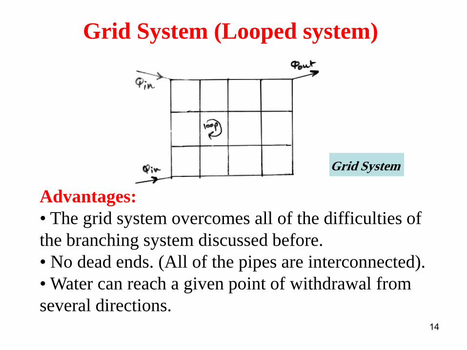
Grid System (Looped system)
Grid System
Advantages:
• The grid system overcomes all of the difficulties of
the branching system discussed before.
• No dead ends. (All of the pipes are interconnected).
• Water can reach a given point of withdrawal from
several directions.

15
Disadvantages:
• Hydraulically far more complicated than branching system (Determination of the pipe sizes is somewhat more complicated) .
• Expensive (consists of a large number of loops).
But, it is the most reliable and used system.

16
Combined System
• It is a combination of both Grid and Branching
systems
• This type is widely used all over the world.
Combined System
17
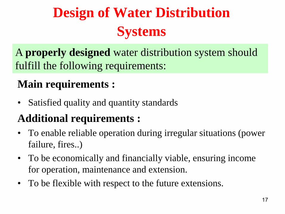
Design of Water Distribution
Systems
Main requirements :
• Satisfied quality and quantity standards
Additional requirements :
• To enable reliable operation during irregular situations (power
failure, fires..)
• To be economically and financially viable, ensuring income
for operation, maintenance and extension.
• To be flexible with respect to the future extensions.
A properly designed water distribution system should
fulfill the following requirements:
18
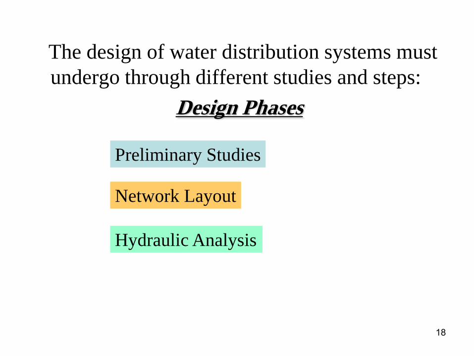
The design of water distribution systems must
undergo through different studies and steps:
Design Phases
Hydraulic Analysis
Preliminary Studies
Network Layout

19
Preliminary Studies:
4.3.A.1 Topographical Studies:
Must be performed before starting the actual design:
1. Contour lines (or controlling elevations).
2. Digital maps showing present (and future) houses,
streets, lots, and so on..
3. Location of water sources so to help locating
distribution reservoirs.
20
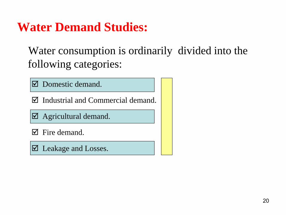
Water Demand Studies:
Water consumption is ordinarily divided into the
following categories:
Domestic demand.
Industrial and Commercial demand.
Agricultural demand.
Fire demand.
Leakage and Losses.
21
Domestic demand
• It is the amount of water used for Drinking, Cocking, Gardening, Car Washing, Bathing, Laundry, Dish Washing, and Toilet Flushing.
• The average water consumption is different from one population to another. In Gaza strip the average consumption is 70 L/capita/day which is very low compared with other countries. For example, it is 250 L/c/day in United States, and it is 180 L/c/day for population live in Cairo (Egypt).
• The average consumption may increase with the increase in standard of living.
• The water consumption varies hourly, daily, and monthly

22
How to predict the increase of population?
The total amount of water for domestic use is a function of:
Population increase
Geometric-increase model Use
P P r n 0 1( ) P0 = recent population
r = rate of population growth
n = design period in years
P = population at the end of the design period.
The total domestic demand can be estimated using:
Qdomestic = Qavg * P
23
Industrial and Commercial demand
• It is the amount of water needed for factories, offices,
and stores….
• Varies from one city to another and from one country
to another
• Hence should be studied for each case separately.
• However, it is sometimes taken as a percentage of the
domestic demand.
24
Agricultural demand
• It depends on the type of crops, soil, climate…
Fire demand
• To resist fire, the network should save a certain
amount of water.
• Many formulas can be used to estimate the amount of
water needed for fire.

25
Fire demand Formulas
)01.01(65 PPQF QF = fire demand l/s P = population in thousands
Q PF 53QF = fire demand l/s P = population in thousands
Q C AF 320*QF = fire demand flow m3/d
A = areas of all stories of the building
under consideration (m2 ) C = constant depending on the type of
construction;
The above formulas can be replaced with local ones
(Amounts of water needed for fire in these formulas are high).
26
Leakage and Losses
• This is “unaccounted for water” (UFW)
• It is attributable to:
Errors in meter readings
Unauthorized connections
Leaks in the distribution system

27
Design Criteria
Are the design limitations required to get the most efficient and economical water-distribution network
Velocity
Pressure
Average Water Consumption

28
Velocity
• Not be lower than 0.6 m/s to prevent
sedimentation
• Not be more than 3 m/s to prevent erosion and
high head losses.
• Commonly used values are 1 - 1.5 m/sec.
29
Pressure
• Pressure in municipal distribution systems ranges from 150-300 kPa in residential districts with structures of four stories or less and 400-500 kPa in commercial districts.
• Also, for fire hydrants the pressure should not be less than 150 kPa (15 m of water).
• In general for any node in the network the pressure should not be less than 25 m of water.
• Moreover, the maximum pressure should be limited to 70 m
of water
30
Pipe sizes • Lines which provide only domestic flow may be as small as 100 mm
(4 in) but should not exceed 400 m in length (if dead-ended) or 600 m if connected to the system at both ends.
• Lines as small as 50-75 mm (2-3 in) are sometimes used in small communities with length not to exceed 100 m (if dead-ended) or 200 m if connected at both ends.
• The size of the small distribution mains is seldom less than 150 mm (6 in) with cross mains located at intervals not more than 180 m.
• In high-value districts the minimum size is 200 mm (8 in) with cross-mains at the same maximum spacing. Major streets are provided with lines not less than 305 mm (12 in) in diameter.

31
Head Losses
• Optimum range is 1-4 m/km.
• Maximum head loss should not exceed 10
m/km.

32
Design Period for Water supply Components
• The economic design period of the components of a
distribution system depends on
• Their life.
• First cost.
• And the ease of expandability.
33
Average Water Consumption
• From the water demand (preliminary) studies,
estimate the average and peak water
consumption for the area.
34
Network Layout
• Next step is to estimate pipe sizes on the basis of water demand and local code requirements.
• The pipes are then drawn on a digital map (using AutoCAD, for example) starting from the water source.
• All the components (pipes, valves, fire hydrants) of the water network should be shown on the lines.

35
Pipe Networks
• A hydraulic model is useful for examining the impact of design and operation decisions.
• Simple systems, such as those discussed in last chapters can be solved using a hand calculator.
• However, more complex systems require more effort even for steady state conditions, but, as in simple systems, the flow and pressure-head distribution through a water distribution system must satisfy the laws of conservation of mass and energy.

36
• The equations to solve Pipe network must
satisfy the following condition:
• The net flow into any junction must be zero
• The net head loss a round any closed loop must
be zero. The HGL at each junction must have one
and only one elevation
• All head losses must satisfy the Moody and
minor-loss friction correlation
Pipe Networks
0Q
37
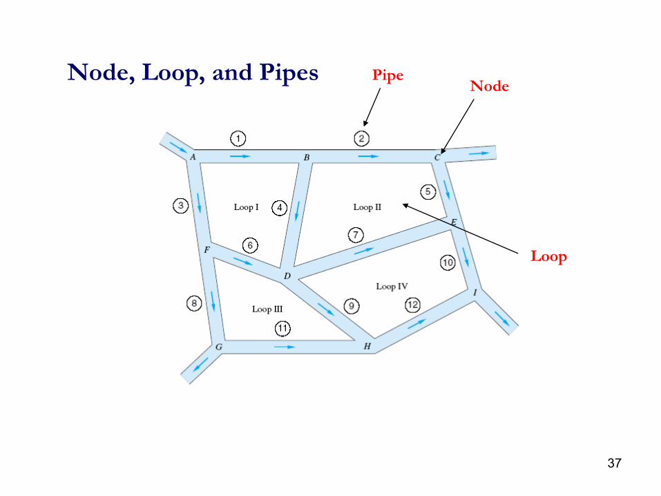
Node, Loop, and Pipes Node
Pipe
Loop
38
After completing all preliminary studies and
layout drawing of the network, one of the
methods of hydraulic analysis is used to
• Size the pipes and
• Assign the pressures and velocities
required.
Hydraulic Analysis

39
Hydraulic Analysis of Water Networks
• The solution to the problem is based on the same
basic hydraulic principles that govern simple and
compound pipes that were discussed previously.
• The following are the most common methods used to
analyze the Grid-system networks:
1. Hardy Cross method.
2. Sections method.
3. Circle method.
4. Computer programs (WaterCAD,Epanet, Loop, Alied...)

40
Hardy Cross Method
• This method is applicable to closed-loop pipe
networks (a complex set of pipes in parallel).
• It depends on the idea of head balance method
• Was originally devised by professor Hardy Cross.
41
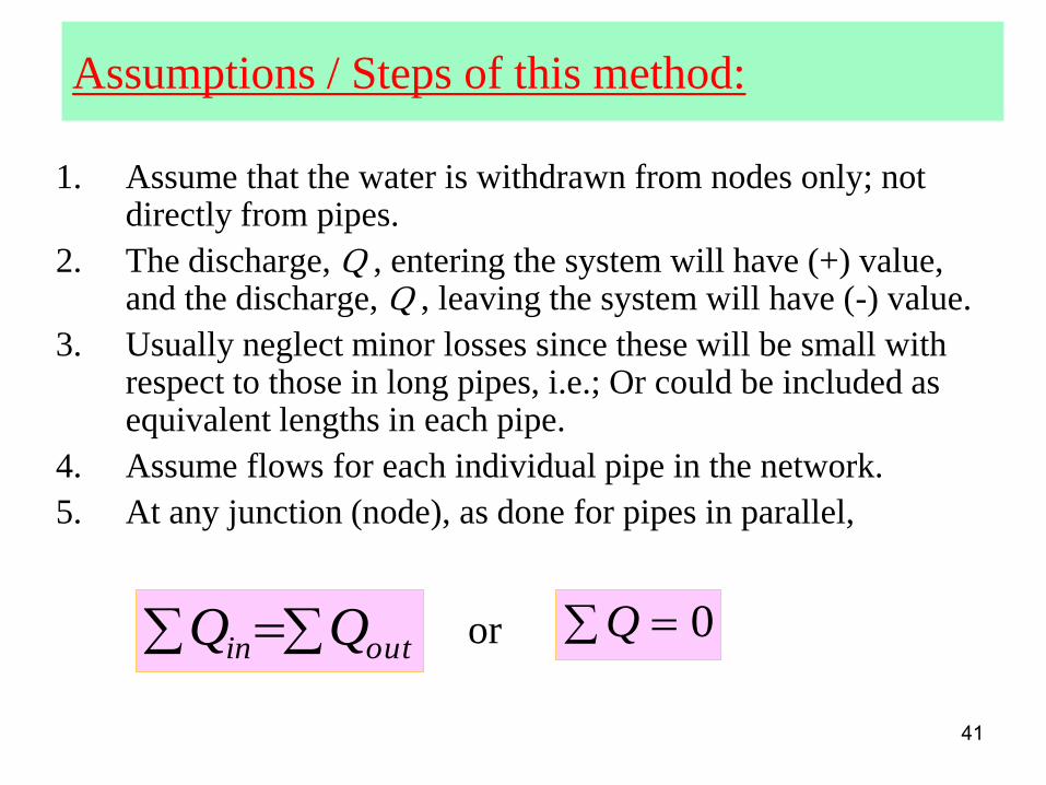
Assumptions / Steps of this method:
1. Assume that the water is withdrawn from nodes only; not directly from pipes.
2. The discharge, Q , entering the system will have (+) value, and the discharge, Q , leaving the system will have (-) value.
3. Usually neglect minor losses since these will be small with respect to those in long pipes, i.e.; Or could be included as equivalent lengths in each pipe.
4. Assume flows for each individual pipe in the network.
5. At any junction (node), as done for pipes in parallel,
outin QQ Q 0or
42
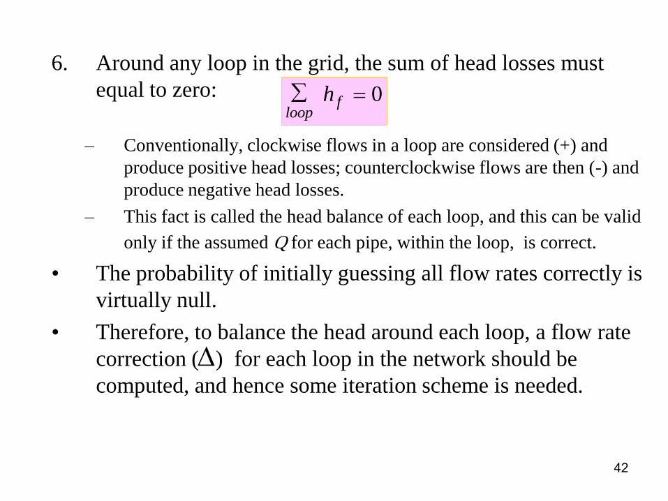
6. Around any loop in the grid, the sum of head losses must
equal to zero:
– Conventionally, clockwise flows in a loop are considered (+) and
produce positive head losses; counterclockwise flows are then (-) and
produce negative head losses.
– This fact is called the head balance of each loop, and this can be valid
only if the assumed Q for each pipe, within the loop, is correct.
• The probability of initially guessing all flow rates correctly is
virtually null.
• Therefore, to balance the head around each loop, a flow rate
correction ( ) for each loop in the network should be
computed, and hence some iteration scheme is needed.
h floop
0

43
7. After finding the discharge correction, (one for each loop) , the assumed discharges Q0 are adjusted and another iteration is carried out until all corrections (values of ) become zero or negligible. At this point the condition of :
is satisfied.
Notes:
• The flows in pipes common to two loops are positive in one loop and negative in the other.
• When calculated corrections are applied, with careful attention to sign, pipes common to two loops receive both corrections.
h floop
0 0.

44
How to find the correction value ( )
WilliamHazenn
ManningDarcyn
kQh n
F
85.1
,2
)1(
)2( oQQ
....
2
1
2& 1
221
f
n
o
n
o
n
o
n
o
n Qnn
nQQkQkkQh
from
1
f n
o
n
o
n nQQkkQh
0
0
1
nn
o
n
loop
n
loop
F
nkQkQkQ
kQh
Neglect terms contains 2
For each loop
45
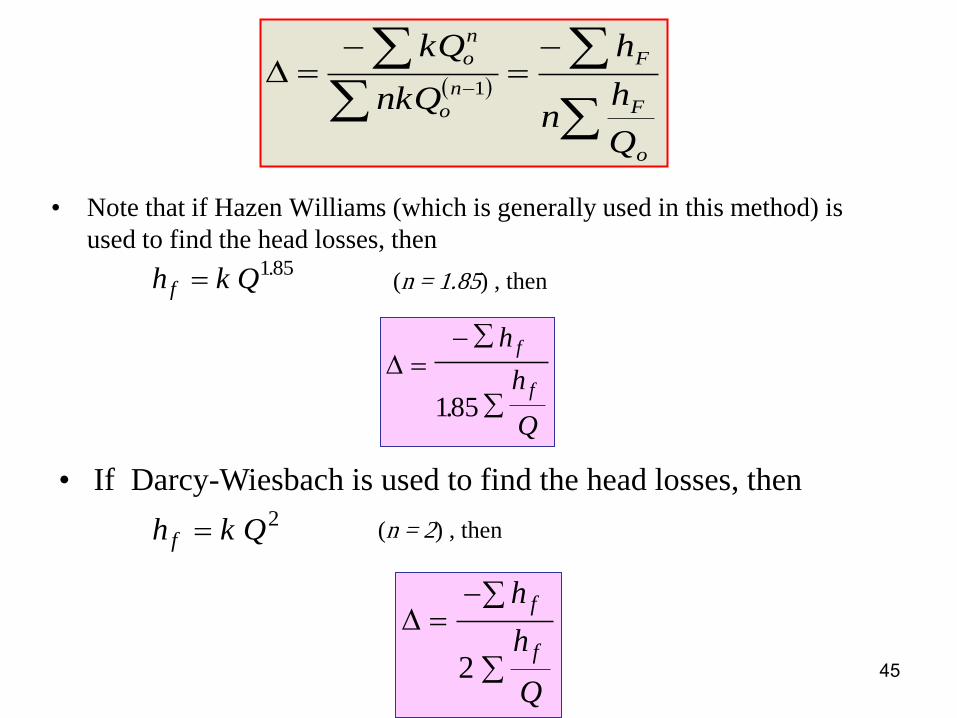
• Note that if Hazen Williams (which is generally used in this method) is
used to find the head losses, then
h k Qf 185.(n = 1.85) , then
h
h
Q
f
f185.
• If Darcy-Wiesbach is used to find the head losses, then
h k Qf 2
h
h
Q
f
f2
(n = 2) , then
o
F
F
n
o
n
o
Q
hn
h
nkQ
kQ
1

46
Example
D L pipe
150mm 305m 1
150mm 305m 2
200mm 610m 3
150mm 457m 4
200mm 153m 5
1
2 3 4
5
37.8 L/s
25.2 L/s
63 L/s
24
11.4
Solve the following pipe network using Hazen William Method CHW =100

47
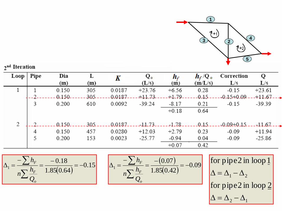
24.0
64.085.1
28.01
o
F
F
Q
hn
h
1002.6
1000
0.71
L/s ,100
0.71
852.1
852.1
87.4
9
852.1
87.4852.1
852.1
87.4852.1
QKh
QD
Lh
Q
DC
Lh
inQCQDC
Lh
f
f
HW
f
HW
HW
f
57.0
43.085.1
45.02
o
F
F
Q
hn
h
1
2 3 4
5
12
21
2 loopin 2 pipefor
1 loopin 2 pipefor
48
15.0
64.085.1
18.01
o
F
F
Q
hn
h
09.042.085.1
07.01
o
F
F
Q
hn
h
1
2 3 4
5
12
21
2 loopin 2 pipefor
1 loopin 2 pipefor
49
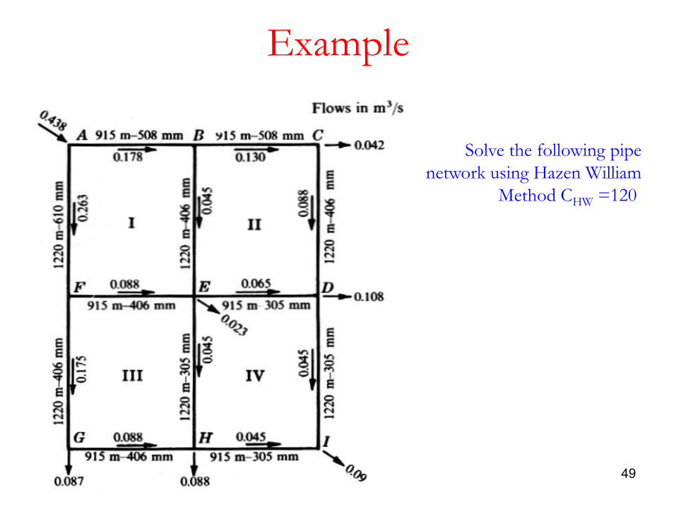
Solve the following pipe
network using Hazen William
Method CHW =120
Example

50
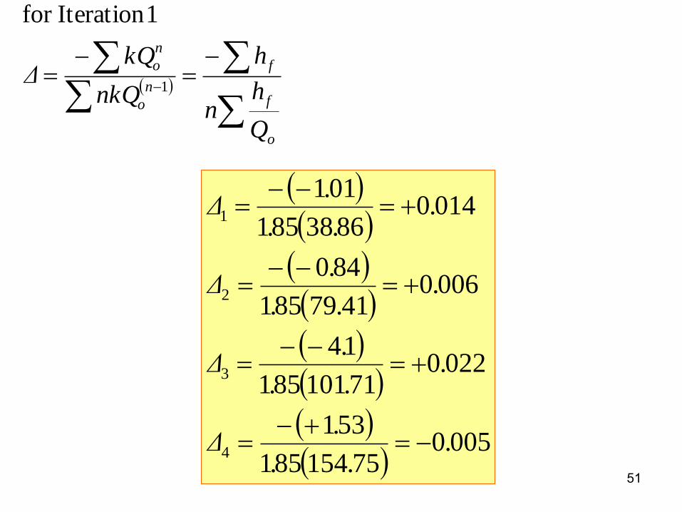
Iteration 1
51
005075154851
531
022071101851
14
00604179851
840
01408638851
011
4
3
2
1
...
.Δ
...
.Δ
...
.Δ
...
.Δ
o
f
f
n
o
n
o
Q
hn
h
nkQ
kQΔ
1
1Iteration for

52
Iteration 2
53
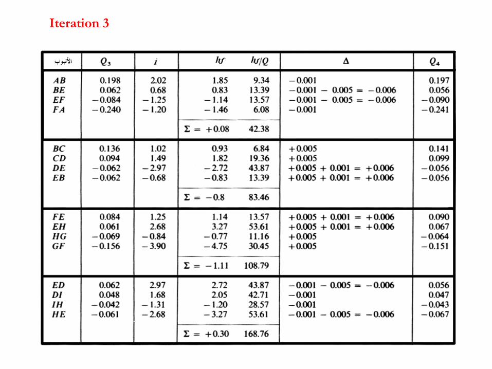
Iteration 3
54
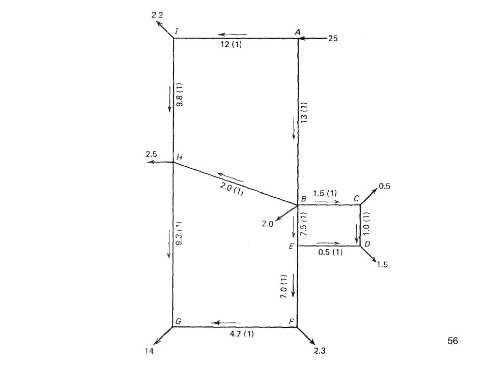
Example
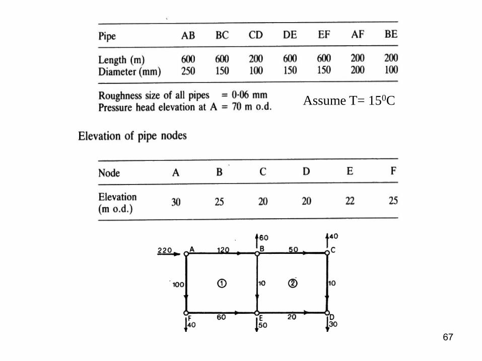
• The figure below represents a simplified pipe network.
• Flows for the area have been disaggregated to the nodes, and a major fire flow has been added at node G.
• The water enters the system at node A.
• Pipe diameters and lengths are shown on the figure.
• Find the flow rate of water in each pipe using the Hazen-Williams equation with CHW = 100.
• Carry out calculations until the corrections are less then 0.2 m3/min.

55
56
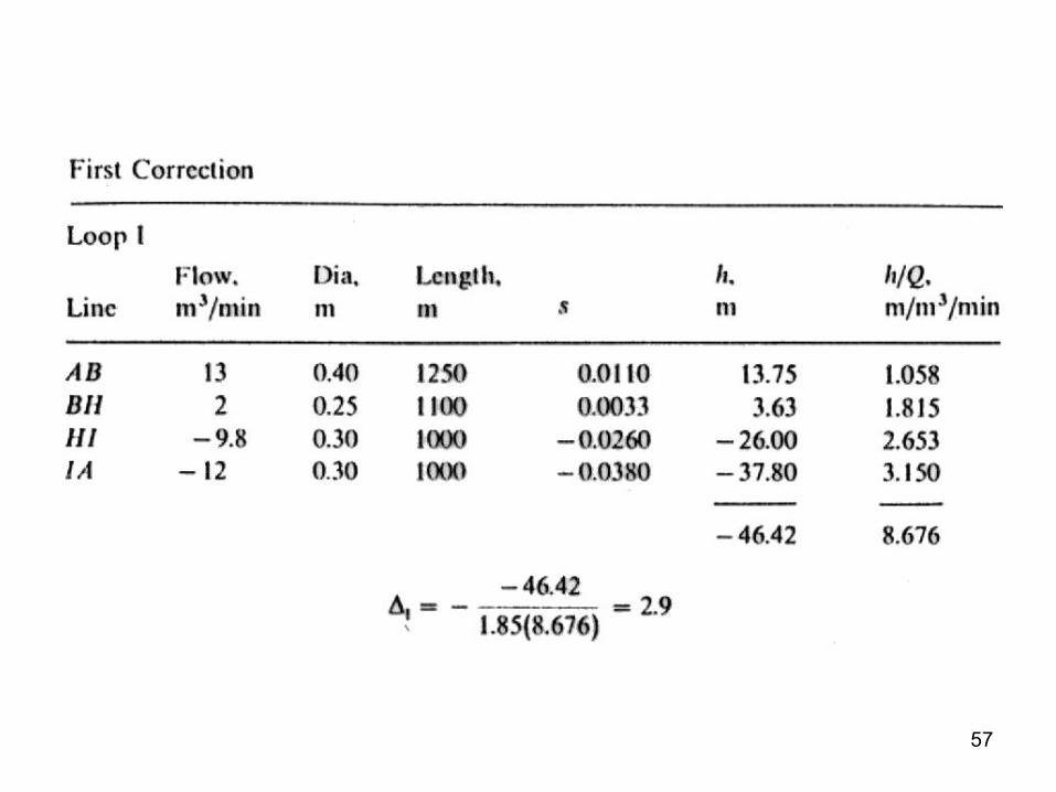
57

58
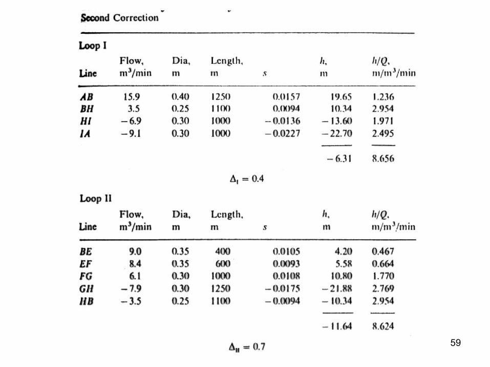
59
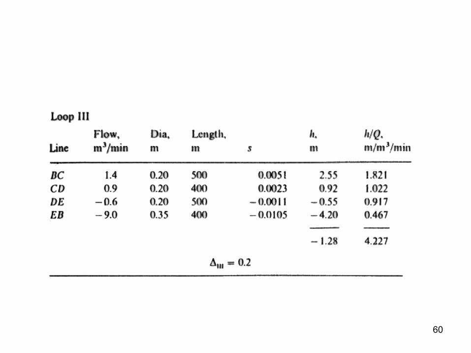
60

61
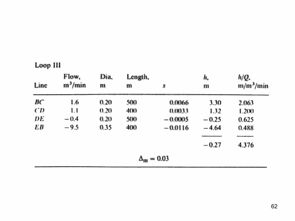
62

63

64
General Notes
• Occasionally the assumed direction of flow will be incorrect. In such cases the method will produce corrections larger than the original flow and in subsequent calculations the direction will be reversed.
• Even when the initial flow assumptions are poor, the convergence will usually be rapid. Only in unusual cases will more than three iterations be necessary.
• The method is applicable to the design of new system or to evaluate the proposed changes in an existing system.
• The pressure calculation in the above example assumes points are at equal elevations. If they are not, the elevation difference must be includes in the calculation.
• The balanced network must then be reviewed to assure that the velocity and pressure criteria are satisfied. If some lines do not meet the suggested criteria, it would be necessary to increase the diameters of these pipes and repeat the calculations.

65
• Assigning clockwise flows and their associated head
losses are positive, the procedure is as follows:
Assume values of Q to satisfy Q = 0.
Calculate HL from Q using hf = K1Q2 .
If hf = 0, then the solution is correct.
If hf 0, then apply a correction factor, Q, to all
Q and repeat from step (2).
For practical purposes, the calculation is usually
terminated when hf < 0.01 m or Q < 1 L/s.
A reasonably efficient value of Q for rapid
convergence is given by;
QH
2
HQ
L
L
Summary
QH
2
HQ
L
L

66
Example
• The following example contains nodes with different
elevations and pressure heads.
• Neglecting minor loses in the pipes, determine:
• The flows in the pipes.
• The pressure heads at the nodes.
67
Assume T= 150C

68
Assume flows magnitude and direction
69
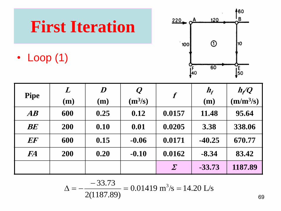
First Iteration
• Loop (1)
Pipe L
(m)
D
(m)
Q
(m3/s) f
hf
(m)
hf/Q
(m/m3/s)
AB 600 0.25 0.12 0.0157 11.48 95.64
BE 200 0.10 0.01 0.0205 3.38 338.06
EF 600 0.15 -0.06 0.0171 -40.25 670.77
FA 200 0.20 -0.10 0.0162 -8.34 83.42
S -33.73 1187.89
L/s20.14/sm01419.0)89.1187(2
73.33 3

70
First Iteration
• Loop (2)
Pipe L
(m)
D
(m)
Q
(m3/s) f
hf
(m)
hf/Q
(m/m3/s)
BC 600 0.15 0.05 0.0173 28.29 565.81
CD 200 0.10 0.01 0.0205 3.38 338.05
DE 600 0.15 -0.02 0.0189 -4.94 246.78
EB 200 0.10 -0.01 0.0205 -3.38 338.05
S 23.35 1488.7
L/s842.7/sm00784.0)7.1488(2
35.23 3

71
Second Iteration
• Loop (1)
Pipe L
(m)
D
(m)
Q
(m3/s) f
hf
(m)
hf/Q
(m/m3/s)
AB 600 0.25 0.1342 0.0156 14.27 106.08
BE 200 0.10 0.03204 0.0186 31.48 982.60
EF 600 0.15 -0.0458 0.0174 -23.89 521.61
FA 200 0.20 -0.0858 0.0163 -6.21 72.33
S 15.65 1682.62
L/s65.4/sm00465.0)62.1682(2
65.15 3
14.20
14.20
14.20 7.84 14.20
72
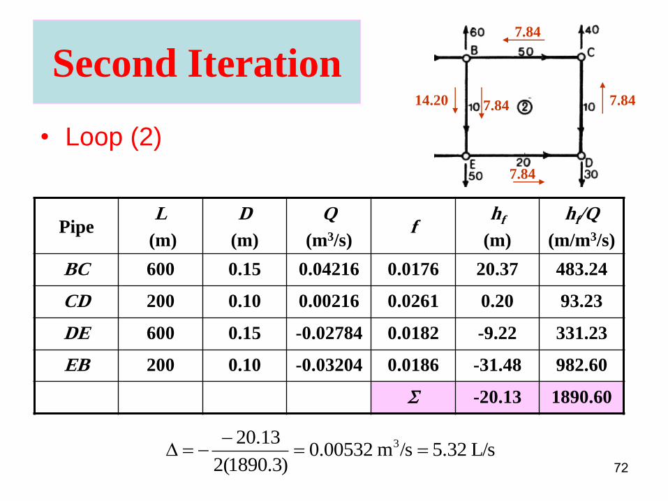
Second Iteration
• Loop (2)
Pipe L
(m)
D
(m)
Q
(m3/s) f
hf
(m)
hf/Q
(m/m3/s)
BC 600 0.15 0.04216 0.0176 20.37 483.24
CD 200 0.10 0.00216 0.0261 0.20 93.23
DE 600 0.15 -0.02784 0.0182 -9.22 331.23
EB 200 0.10 -0.03204 0.0186 -31.48 982.60
S -20.13 1890.60
L/s32.5/sm00532.0)3.1890(2
13.20 3
14.20 7.84
7.84
7.84
7.84

73
Third Iteration
• Loop (1)
Pipe L
(m)
D
(m)
Q
(m3/s) f
hf
(m)
hf/Q
(m/m3/s)
AB 600 0.25 0.1296 0.0156 13.30 102.67
BE 200 0.10 0.02207 0.0190 15.30 693.08
EF 600 0.15 -0.05045 0.0173 -28.78 570.54
FA 200 0.20 -0.09045 0.0163 -6.87 75.97
S -7.05 1442.26
L/s44.2/sm00244.0)26.1442(2
05.7 3

74
Third Iteration
• Loop (2)
Pipe L
(m)
D
(m)
Q
(m3/s) f
hf
(m)
hf/Q
(m/m3/s)
BC 600 0.15 0.04748 0.0174 25.61 539.30
CD 200 0.10 0.00748 0.0212 1.96 262.11
DE 600 0.15 -0.02252 0.0186 -6.17 274.07
EB 200 0.10 -0.02207 0.0190 -15.30 693.08
S 6.1 1768.56
L/s72.1/sm00172.0)56.1768(2
1.6 3
75
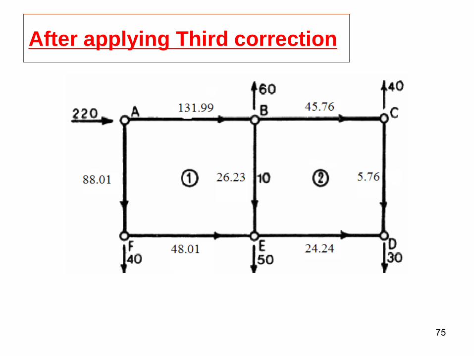
After applying Third correction
76
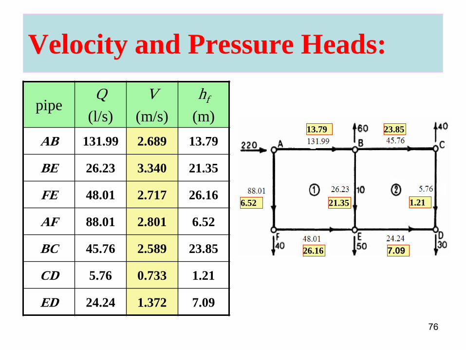
Velocity and Pressure Heads:
pipe Q
(l/s)
V
(m/s)
hf
(m)
AB 131.99 2.689 13.79
BE 26.23 3.340 21.35
FE 48.01 2.717 26.16
AF 88.01 2.801 6.52
BC 45.76 2.589 23.85
CD 5.76 0.733 1.21
ED 24.24 1.372 7.09
1.21 21.35
13.79 23.85
6.52
26.16 7.09
77
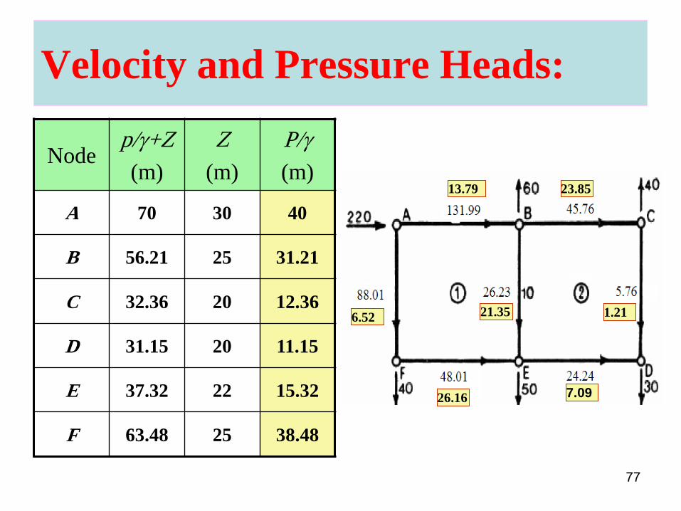
Velocity and Pressure Heads:
Node p/g+Z
(m)
Z
(m)
P/g
(m)
A 70 30 40
B 56.21 25 31.21
C 32.36 20 12.36
D 31.15 20 11.15
E 37.32 22 15.32
F 63.48 25 38.48
1.21 21.35
13.79 23.85
6.52
26.16 7.09
78
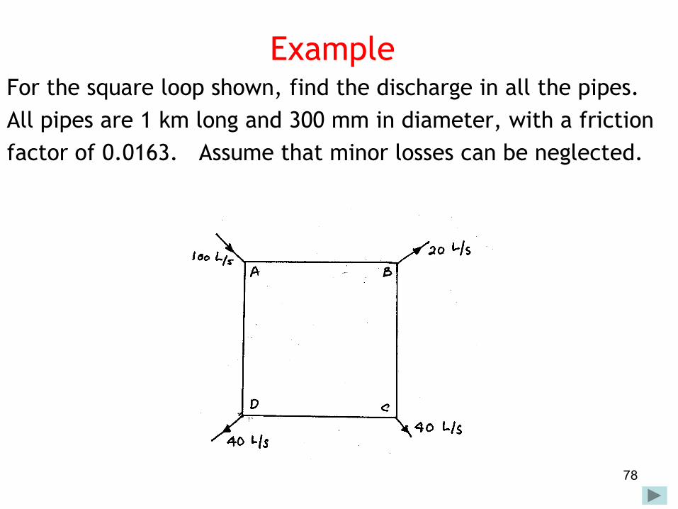
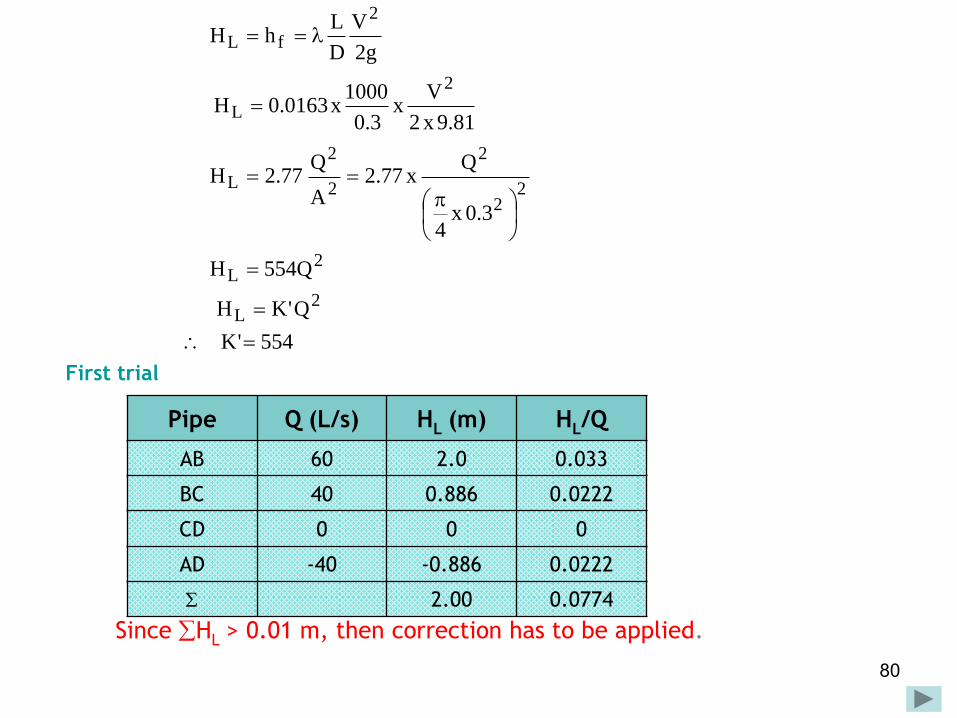
Example For the square loop shown, find the discharge in all the pipes.
All pipes are 1 km long and 300 mm in diameter, with a friction
factor of 0.0163. Assume that minor losses can be neglected.

79
•Solution:
Assume values of Q to satisfy continuity equations all at nodes.
The head loss is calculated using; HL = K1Q2
HL = hf + hLm
But minor losses can be neglected: hLm = 0
Thus HL = hf
Head loss can be calculated using the Darcy-Weisbach equation
g2
V
D
Lh
2
f
80
First trial
Since HL > 0.01 m, then correction has to be applied.
554'K
Q'KH
Q554H
3.0x4
Qx77.2
A
Q77.2H
81.9x2
Vx
3.0
1000x0163.0H
g2
V
D
LhH
2L
2L
22
2
2
2
L
2
L
2
fL
Pipe Q (L/s) HL (m) HL/Q
AB 60 2.0 0.033
BC 40 0.886 0.0222
CD 0 0 0
AD -40 -0.886 0.0222
S 2.00 0.0774

81
Second trial
Since HL ≈ 0.01 m, then it is OK.
Thus, the discharge in each pipe is as follows (to the nearest integer).
s/L92.120774.0x2
2
QH
2
HQ
L
L
Pipe Q (L/s) HL (m) HL/Q
AB 47.08 1.23 0.0261
BC 27.08 0.407 0.015
CD -12.92 -0.092 0.007
AD -52.92 -1.555 0.0294
S -0.0107 0.07775
Pipe Discharge
(L/s)
AB 47
BC 27
CD -13
AD -53

82
:قال اهلل تعالى
كر ذرجال ال تلهيهم تجارة وال بيع عن اهلل

83
حب الدنيا
اعمم أّن جمود العين من قسوة القمب،
وقسوة القمب من كثرة الذنوب، وكثرة الذنوب من نسيان الموت،
ونسيان الموت من طول األمل، وطول األمل من شدة الحرص،
وشدة الحرص من حب الدنيا، .خطيئة وحب الدنيا رأس كل
84
تهادوا تحابوا
ولى قّل سعرها ال تبخل بالهذية
فقيمتها معنىية اكثر من مادية

85
تقوى هللا مفتاح كل نجاح
“ومن يتق هللا يجعل له مخرجاً ويرزقه من حيث ال يحتسب”