Embed Size (px)
Citation preview
Application of the Finite Element Method Using MARC and Mentat 4-1
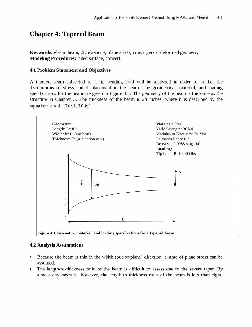
Chapter 4: Tapered Beam Keywords: elastic beam, 2D elasticity, plane stress, convergence, deformed geometry Modeling Procedures: ruled surface, convert 4.1 Problem Statement and Objectives A tapered beam subjected to a tip bending load will be analyzed in order to predict the distributions of stress and displacement in the beam. The geometrical, material, and loading specifications for the beam are given in Figure 4.1. The geometry of the beam is the same as the structure in Chapter 3. The thickness of the beam is 2h inches, where h is described by the equation: h x x= − +4 06 003 2. .
4.2 Analysis Assumptions • Because the beam is thin in the width (out-of-plane) direction, a state of plane stress can be
assumed. • The length-to-thickness ratio of the beam is difficult to assess due to the severe taper. By
almost any measure, however, the length-to-thickness ratio of the beam is less than eight.
Geometry: Material: Steel Length: L=10” Yield Strength: 36 ksi Width: b=1” (uniform) Modulus of Elasticity: 29 Msi Thickness: 2h (a function of x) Poisson’s Ratio: 0.3 Density = 0.0088 slugs/in3 Loading: Tip Load: P=10,000 lbs
Figure 4.1 Geometry, material, and loading specifications for a tapered beam.
P
2h
L
x
Application of the Finite Element Method Using MARC and Mentat 4-2
Hence, it is unclear whether thin beam theory will accurately predict the response of the beam. Therefore, both a 2D plane stress elasticity analysis and a thin elastic beam analysis will be performed.
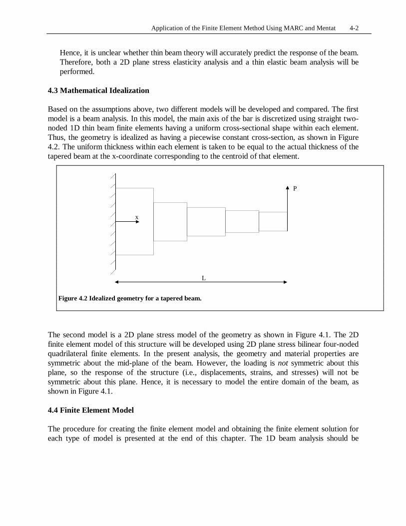
4.3 Mathematical Idealization Based on the assumptions above, two different models will be developed and compared. The first model is a beam analysis. In this model, the main axis of the bar is discretized using straight two-noded 1D thin beam finite elements having a uniform cross-sectional shape within each element. Thus, the geometry is idealized as having a piecewise constant cross-section, as shown in Figure 4.2. The uniform thickness within each element is taken to be equal to the actual thickness of the tapered beam at the x-coordinate corresponding to the centroid of that element.
The second model is a 2D plane stress model of the geometry as shown in Figure 4.1. The 2D finite element model of this structure will be developed using 2D plane stress bilinear four-noded quadrilateral finite elements. In the present analysis, the geometry and material properties are symmetric about the mid-plane of the beam. However, the loading is not symmetric about this plane, so the response of the structure (i.e., displacements, strains, and stresses) will not be symmetric about this plane. Hence, it is necessary to model the entire domain of the beam, as shown in Figure 4.1. 4.4 Finite Element Model The procedure for creating the finite element model and obtaining the finite element solution for each type of model is presented at the end of this chapter. The 1D beam analysis should be
Figure 4.2 Idealized geometry for a tapered beam.
P
L
x
Application of the Finite Element Method Using MARC and Mentat 4-3
performed three times, each with a different mesh. Meshes consisting of 2, 4 and 6 elements should be developed. The 2D analysis should be performed only one time, using the mesh described within the procedure. 4.5 Model Validation Simple hand calculations can be performed to estimate the stresses and deflections in this beam structure. The results of these calculations should be used to assess the validity of the finite element results (i.e., to make sure that the finite element results are reasonable and do not contain any large error due to a simple mistake in the model). The vertical displacement at the end of the bar can be approximated by assuming the bar is of uniform cross-sectional shape. The cross-sectional shape used in this calculation may be, for example, the cross-sectional shape at the mid-point of the bar (at x = 5”). Then the vertical displacement can be estimated using the well-known relation:
EI
PL
3
3
=δ
where δ is the tip displacement of the bar, I is the (uniform) second moment of the cross-sectional area about the bending axis, and the other parameters are defined in Figure 4.1. Note that the above relation depends strongly on the value of I, which varies along the length of the actual beam. Thus, the approximation above cannot be expected to be accurate in the current situation, but it should provide a reasonable first-order estimate. The axial stress at any cross-section in the beam can be estimated by neglecting all other stress components and assuming that the axial stress is linearly distributed over the cross-section according to beam theory. From equilibrium, it is found that the resultant moment M at any cross-section is P(L-x), so the axial stress can be estimated using the relation:
( )I
yxLP
I
My −==σ
where I is the actual second moment of the area at the cross-section under consideration and y is the vertical coordinate with its origin at the centroid of the beam. 3.6 Post Processing A total of four finite element models were developed – three using 1D two-noded thin beam elements, and one using 2D four-noded bilinear plane stress elements. Based on the results of these analyses, perform and submit the following postprocessing steps.

Application of the Finite Element Method Using MARC and Mentat 4-4
(1) Complete the following table:
Model ID Tip Displacement Maximum Stress at x = 5” 1D – two elements 1D – four elements 1D – six elements 2D – plane stress elements Validation hand calculation (2) Create a plot of the distribution of vertical displacement along the x-axis as predicted by the four models. Put all of the results on a single plot so that comparisons among the solutions can be made. (3) Create a plot of the distribution of maximum axial stress along the x-axis as predicted by the four models. Put all of the results on a single plot so that comparisons among the solutions can be made. For the beam element models, use hand calculations to calculate the stress based on the predicted bending moment at each node. (4) Comment on the convergence of displacement and stress in the 1D beam solutions. (5) Comment on the validity of the solutions. Show the hand calculations. (6) Include the following plots in the final report: For each of the three 1D models, include a "numerics" plot for:
(a) y-displacement (b) x-component of stress
For the 2D model, include a stress contour plot for: (a) x-component of stress (b) y-component of stress (c) y-displacement
Application of the Finite Element Method Using MARC and Mentat 4-5
TAPERED BEAM WITH A TIP LOAD -- using two elastic beam elements 1. Add points to define geometry. 1a. Add points.
<ML> MAIN MENU / MESH GENERATION <ML> MAIN MENU / MESH GENERATION / PTS ADD
Enter the coordinates at the command line, one point per line with a space separating each coordinate.
> 0.0 0.0 0.0 > 5.0 0.0 0.0 > 10.0 0.0 0.0
The points may not appear in the Graphics window because Mentat does not yet know the size of the model being built. When the FILL command in the static menu is executed, Mentat calculates a bounding box for the model and fits the model inside the Grapics window.
<ML> STATIC MENU / FILL
The points should now be visible in the Graphics window.
1b. Display point labels.
<ML> STATIC MENU / PLOT <ML> STATIC MENU / PLOT / POINTS SETTINGS <ML> STATIC MENU / PLOT / POINTS SETTINGS / LABELS <ML> STATIC MENU / PLOT / POINTS SETTINGS / LABELS / REDRAW
1c. Return to MESH GENERATION menu.
<MR> or <ML> RETURN
Application of the Finite Element Method Using MARC and Mentat 4-6
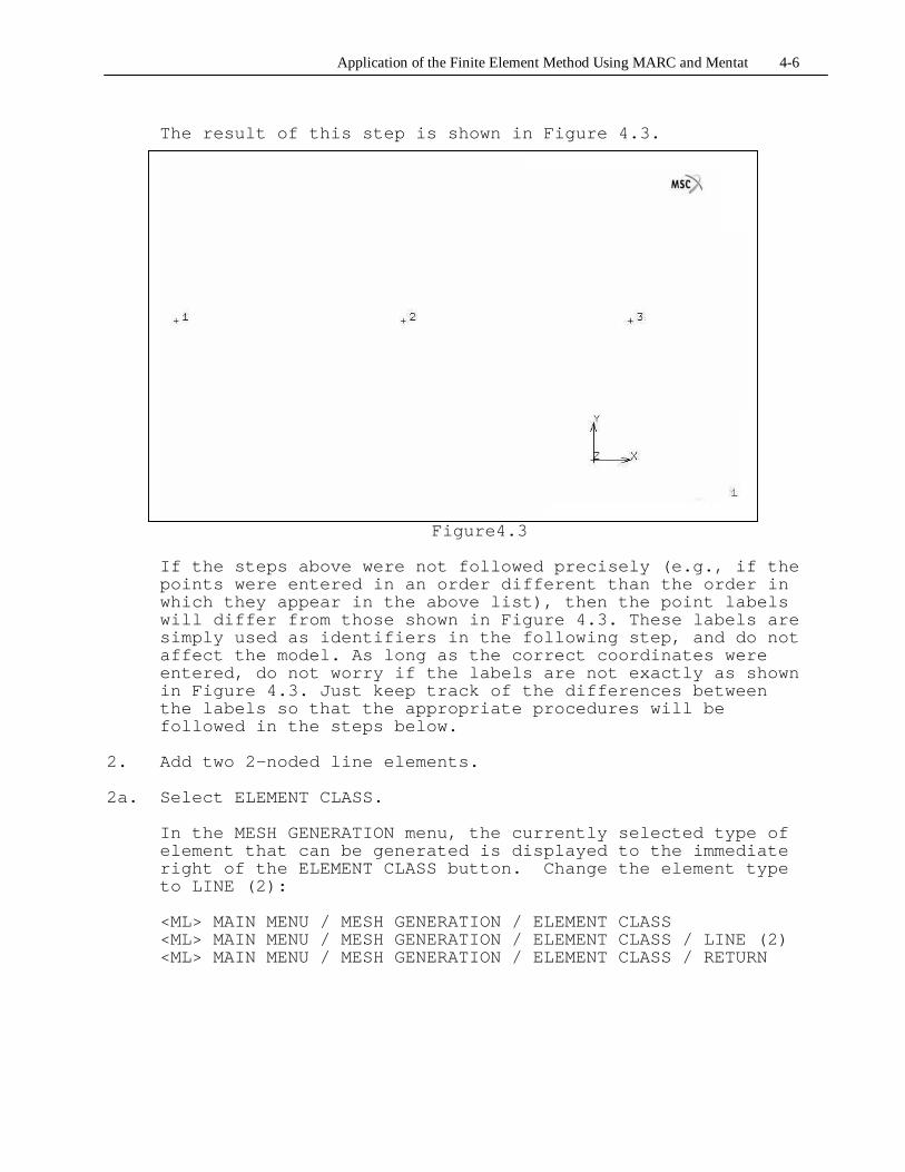
The result of this step is shown in Figure 4.3.
Figure4.3 If the steps above were not followed precisely (e.g., if the points were entered in an order different than the order in which they appear in the above list), then the point labels will differ from those shown in Figure 4.3. These labels are simply used as identifiers in the following step, and do not affect the model. As long as the correct coordinates were entered, do not worry if the labels are not exactly as shown in Figure 4.3. Just keep track of the differences between the labels so that the appropriate procedures will be followed in the steps below.
2. Add two 2-noded line elements. 2a. Select ELEMENT CLASS.
In the MESH GENERATION menu, the currently selected type of element that can be generated is displayed to the immediate right of the ELEMENT CLASS button. Change the element type to LINE (2):
<ML> MAIN MENU / MESH GENERATION / ELEMENT CLASS <ML> MAIN MENU / MESH GENERATION / ELEMENT CLASS / LINE (2) <ML> MAIN MENU / MESH GENERATION / ELEMENT CLASS / RETURN
Application of the Finite Element Method Using MARC and Mentat 4-7
2b. Create a line element from point 1 to point 2 and from point 2 to point 3.
<ML> MAIN MENU / MESH GENERATION / ELEMS ADD
<ML> to select point 1 and then point 2 to create an element
from point 1 to point 2. <ML> to select point 2 and then point 3 to create an element
from point 2 to point 3. 2c. Turn off point labels.
<ML> STATIC MENU / PLOT / POINTS SETTINGS <ML> STATIC MENU / PLOT / POINTS SETTINGS / LABELS <ML> STATIC MENU / PLOT / POINTS SETTINGS / LABELS / REDRAW
2d. Return to MESH GENERATION menu.
<MR> or <ML> RETURN
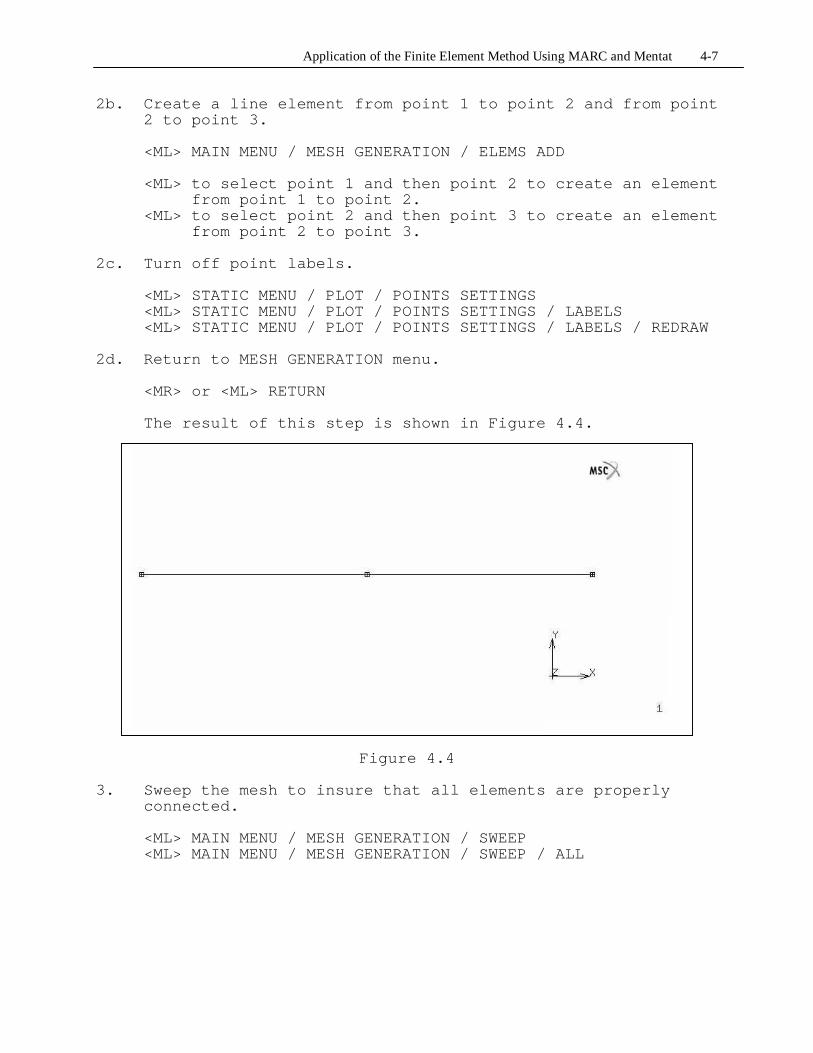
The result of this step is shown in Figure 4.4.
Figure 4.4
3. Sweep the mesh to insure that all elements are properly connected.
<ML> MAIN MENU / MESH GENERATION / SWEEP <ML> MAIN MENU / MESH GENERATION / SWEEP / ALL
Application of the Finite Element Method Using MARC and Mentat 4-8
Note: Duplicate geometrical and mesh entities will be deleted so that proper mesh connectivity is achieved.
Return to MESH GENERATION menu.
<MR> or <ML> RETURN
4. Add boundary conditions. 4a. Specify the constraint condition on the left end of the
model. 4a1. Set up a new boundary condition set.
<ML> MAIN MENU / BOUNDARY CONDITIONS <ML> MAIN MENU / BOUNDARY CONDITIONS / MECHANICAL <ML> MAIN MENU / BOUNDARY CONDITIONS / MECHANICAL / NEW <ML> MAIN MENU / BOUNDARY CONDITIONS / MECHANICAL / NAME
At the command line, enter a name for this boundary condition set.
> FixedPoint
4a2. Define the nature of the boundary condition.
<ML> MAIN MENU / BOUNDARY CONDITIONS / MECHANICAL / FIXED-DISPLACEMENT
Note: Because beam elements have a total of six DOFs (three displacements and three rotations) at each node, it is necessary to constrain the displacements and rotations in all three directions at the left edge of the model so as to restrain all possible rigid body modes.
<ML> MAIN MENU / BOUNDARY CONDITIONS / MECHANICAL /
FIXED-DISPLACEMENT / DISPLACEMENT X <ML> MAIN MENU / BOUNDARY CONDITIONS / MECHANICAL /
FIXED-DISPLACEMENT / DISPLACEMENT Y <ML> MAIN MENU / BOUNDARY CONDITIONS / MECHANICAL /
FIXED-DISPLACEMENT / DISPLACEMENT Z <ML> MAIN MENU / BOUNDARY CONDITIONS / MECHANICAL /
FIXED-DISPLACEMENT / ROTATION X <ML> MAIN MENU / BOUNDARY CONDITIONS / MECHANICAL /
FIXED-DISPLACEMENT / ROTATION Y <ML> MAIN MENU / BOUNDARY CONDITIONS / MECHANICAL /
FIXED-DISPLACEMENT / ROTATION Z
The small box to the immediate left of the DISPLACEMENT X, Y and Z and ROTATION X, Y and Z buttons should now be
Application of the Finite Element Method Using MARC and Mentat 4-9
highlighted. The “0” that appears to the right of these buttons is the imposed value of the displacement or rotation. If a component of displacement or rotation is non-zero, then the actual value of the displacement or rotation should be entered here.
<ML> MAIN MENU / BOUNDARY CONDITIONS / MECHANICAL /
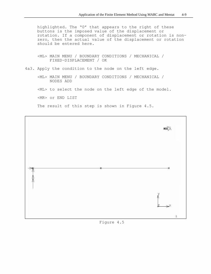
FIXED-DISPLACEMENT / OK 4a3. Apply the condition to the node on the left edge.
<ML> MAIN MENU / BOUNDARY CONDITIONS / MECHANICAL / NODES ADD
<ML> to select the node on the left edge of the model.
<MR> or END LIST
The result of this step is shown in Figure 4.5.
Figure 4.5
Application of the Finite Element Method Using MARC and Mentat 4-10
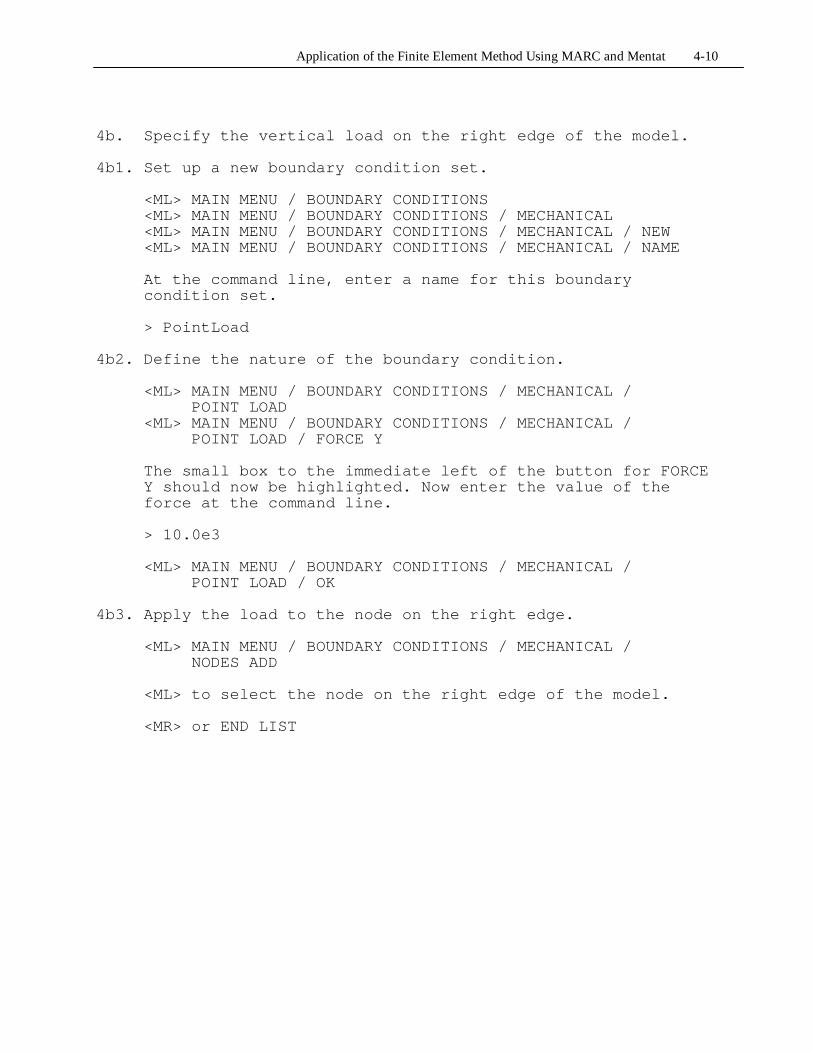
4b. Specify the vertical load on the right edge of the model. 4b1. Set up a new boundary condition set.
<ML> MAIN MENU / BOUNDARY CONDITIONS <ML> MAIN MENU / BOUNDARY CONDITIONS / MECHANICAL <ML> MAIN MENU / BOUNDARY CONDITIONS / MECHANICAL / NEW <ML> MAIN MENU / BOUNDARY CONDITIONS / MECHANICAL / NAME
At the command line, enter a name for this boundary condition set.
> PointLoad
4b2. Define the nature of the boundary condition.
<ML> MAIN MENU / BOUNDARY CONDITIONS / MECHANICAL / POINT LOAD
<ML> MAIN MENU / BOUNDARY CONDITIONS / MECHANICAL / POINT LOAD / FORCE Y
The small box to the immediate left of the button for FORCE Y should now be highlighted. Now enter the value of the force at the command line. > 10.0e3
<ML> MAIN MENU / BOUNDARY CONDITIONS / MECHANICAL /
POINT LOAD / OK 4b3. Apply the load to the node on the right edge.
<ML> MAIN MENU / BOUNDARY CONDITIONS / MECHANICAL / NODES ADD
<ML> to select the node on the right edge of the model.
<MR> or END LIST
Application of the Finite Element Method Using MARC and Mentat 4-11
The result of this step is shown in Figure 4.6.
Figure4.6
4c. Display all boundary conditions for verification.
<ML> MAIN MENU / BOUNDARY CONDITIONS / ID BOUNDARY CONDS
After verifying that boundary conditions have been applied properly, turn off the boundary condition ID's by repeating the last command.
4d. Return to the MAIN menu.
<ML> MAIN MENU / BOUNDARY CONDITIONS / MAIN 5. Specify the material properties of each element. 5a. Set up a new material property set.
<ML> MAIN MENU / MATERIAL PROPERTIES <ML> MAIN MENU / MATERIAL PROPERTIES / NEW <ML> MAIN MENU / MATERIAL PROPERTIES / NAME
At the command line, enter a name for this material property set.
> Steel
Application of the Finite Element Method Using MARC and Mentat 4-12
5b. Define the nature of the material.
<ML> MAIN MENU / MATERIAL PROPERTIES / ISOTROPIC <ML> MAIN MENU / MATERIAL PROPERTIES / ISOTROPIC /
YOUNG'S MODULUS
> 29.0e6
Note: Only Young's modulus needs to be specified for this problem. Beam theory is based on 1D stress-strain relations.
<ML> MAIN MENU / MATERIAL PROPERTIES / ISOTROPIC / OK
5c. Apply the material properties to all elements.
<ML> MAIN MENU / MATERIAL PROPERTIES / ELEMENTS ADD
Since the properties are being applied to all elements in the model, the simplest way to select the elements is to use the ALL EXISTING option.
<ML> ALL: EXIST.
5d. Display all material properties for verification.
<ML> MAIN MENU / MATERIAL PROPERTIES / ID MATERIALS
After verifying that material properties have been applied properly, turn off the material property ID's by repeating the last command.
5e. Return to the MAIN menu.
<ML> MAIN MENU / MATERIAL PROPERTIES / MAIN 6. Specify the geometrical properties of each element. For a
beam element, it is necessary to specify (i) the cross-sectional area, (ii) the second moments of area (Ixx, Iyy) about the two local (principal) axes of the cross-section, and (iii) a vector that defines the direction of the local X-axis.
Note that a local coordinate system must be defined for each beam element. All geometric properties are then defined with respect to this local coordinate system. By default in MARC, the local Z-axis is taken along the length of the element, and the local X- and Y-axes are taken in the plane of the cross-section of the beam element. The first principal axis is called the “LOCAL X-AXIS” and the second principal axis

Application of the Finite Element Method Using MARC and Mentat 4-13
is called the “LOCAL Y-AXIS.” The local X-axis is the axis about which Ixx is calculated. In the present analysis, the local X-axis is taken to be the same as the global Z-axis (positive out of the computer screen). According to the right-hand rule, the local Y-axis will automatically be taken as the negative global Y-axis. So the vector defining the local X-axis is (0,0,1).
6a. Specify geometrical properties for element one. 6a1. Set up a new geometric property set.
<ML> MAIN MENU / GEOMETRIC PROPERTIES <ML> MAIN MENU / GEOMETRIC PROPERTIES / NEW <ML> MAIN MENU / GEOMETRIC PROPERTIES / NAME
At the command line, enter a name for this geometric property set.
> X1
6a2. Define the geometric properties.
<ML> MAIN MENU / GEOMETRIC PROPERTIES / 3D <ML> MAIN MENU / GEOMETRIC PROPERTIES / 3D / ELASTIC BEAM <ML> MAIN MENU / GEOMETRIC PROPERTIES / 3D / ELASTIC BEAM /
AREA
The cross-sectional area of element one is taken as the cross-sectional area of the bar at the geometric centroid of the element (i.e., at x=2.5).
> 5.375 <ML> MAIN MENU / GEOMETRIC PROPERTIES / 3D / ELASTIC BEAM /
Ixx The second moment of the area about the local x-axis (Ixx) is calculated as Ixx = (b)(h^3)/12, where b = 1 and h = 5.375. > 12.94 <ML> MAIN MENU / GEOMETRIC PROPERTIES / 3D / ELASTIC BEAM /
Iyy
The second moment of the area about the local y-axis (Iyy) is calculated as Iyy = (b)(h^3)/12, where b = 5.375 and h = 1.

Application of the Finite Element Method Using MARC and Mentat 4-14
> 0.4479 The local X-axis is defined as being parallel to the global Z-axis. So this vector is (0,0,1). <ML> MAIN MENU / GEOMETRIC PROPERTIES / 3D / ELASTIC BEAM /
X > 0 <ML> MAIN MENU / GEOMETRIC PROPERTIES / 3D / ELASTIC BEAM /
Y > 0 <ML> MAIN MENU / GEOMETRIC PROPERTIES / 3D / ELASTIC BEAM /
Z > 1 <ML> MAIN MENU / GEOMETRIC PROPERTIES / 3D / ELASTIC BEAM /
OK 6a3. Apply the geometric property to element one.
<ML> MAIN MENU / GEOMETRIC PROPERTIES / 3D / ELEMENTS ADD
<ML> on element 1 (on the left side of the model). <MR> or END LIST
6b. Specify cross-sectional area for element two. 6b1. Set up a new geometric property set.
<ML> MAIN MENU / GEOMETRIC PROPERTIES <ML> MAIN MENU / GEOMETRIC PROPERTIES / NEW <ML> MAIN MENU / GEOMETRIC PROPERTIES / NAME
At the command line, enter a name for this geometric property set.
> X2
6b2. Define the geometric properties.
<ML> MAIN MENU / GEOMETRIC PROPERTIES / 3D <ML> MAIN MENU / GEOMETRIC PROPERTIES / 3D / ELASTIC BEAM
Application of the Finite Element Method Using MARC and Mentat 4-15
<ML> MAIN MENU / GEOMETRIC PROPERTIES / 3D / ELASTIC BEAM / AREA
The cross-sectional area of element two is taken as the cross-sectional area of the bar at the geometric centroid of the element (i.e., at x=7.5).
> 2.375 <ML> MAIN MENU / GEOMETRIC PROPERTIES / 3D / ELASTIC BEAM /
Ixx The second moment of the area about the local x-axis (Ixx) is calculated as Ixx = (b)(h^3)/12, where b = 1 and h = 2.375. > 1.116 <ML> MAIN MENU / GEOMETRIC PROPERTIES / 3D / ELASTIC BEAM /
Iyy
The second moment of the area about the local y-axis (Iyy) is calculated as Iyy = (b)(h^3)/12, where b = 2.375 and h = 1. > 0.1979 The local X-axis is defined as being parallel to the global Z-axis. So this vector is (0,0,1). <ML> MAIN MENU / GEOMETRIC PROPERTIES / 3D / ELASTIC BEAM /
X > 0 <ML> MAIN MENU / GEOMETRIC PROPERTIES / 3D / ELASTIC BEAM /
Y > 0 <ML> MAIN MENU / GEOMETRIC PROPERTIES / 3D / ELASTIC BEAM /
Z > 1 <ML> MAIN MENU / GEOMETRIC PROPERTIES / 3D / ELASTIC BEAM /
OK 6b3. Apply the geometric property to element two.
Application of the Finite Element Method Using MARC and Mentat 4-16
<ML> MAIN MENU / GEOMETRIC PROPERTIES / 3D / ELEMENTS ADD
<ML> on element 2 (on the right side of the model). <MR> or END LIST
6c. Display all geometric properties for verification.
<ML> MAIN MENU / GEOMETRIC PROPERTIES / ID GEOMETRIES
After verifying that geometric properties have been applied properly, turn off the geometric property ID's by repeating the last command.
6d. Return to the MAIN menu.
<ML> MAIN MENU / GEOMETRIC PROPERTIES / MAIN 7. Prepare the loadcase.
<ML> MAIN MENU / LOADCASES <ML> MAIN MENU / LOADCASES / MECHANICAL <ML> MAIN MENU / LOADCASES / MECHANICAL / STATIC <ML> MAIN MENU / LOADCASES / MECHANICAL / STATIC / LOADS
Verify that all loads (i.e., boundary constraints and point
load) created in step 4 are selected. The small box to the immediate left of all selected loads will be highlighted. If they are not already selected, then select them using the <ML>.
<ML> MAIN MENU / LOADCASES / MECHANICAL / STATIC /
LOADS / OK <ML> MAIN MENU / LOADCASES / MECHANICAL / STATIC / OK <ML> MAIN MENU / LOADCASES / MECHANICAL / MAIN
8. Prepare the job for execution. 8a. Specify the analysis class and select loadcases.
<ML> MAIN MENU / JOBS <ML> MAIN MENU / JOBS / MECHANICAL <ML> MAIN MENU / JOBS / MECHANICAL / lcase1
8b. Select the analysis dimension.
<ML> MAIN MENU / JOBS / MECHANICAL / 3D
Application of the Finite Element Method Using MARC and Mentat 4-17
8c. Select the desired output variables. In this case, we choose stress as well as the resulting bending moments, shear forces, and torsional moment.
<ML> MAIN MENU / JOBS / MECHANICAL / JOB RESULTS <ML> MAIN MENU / JOBS / MECHANICAL / JOB RESULTS
/stress <ML> MAIN MENU / JOBS / MECHANICAL / JOB RESULTS
/bm_axi_for <ML> MAIN MENU / JOBS / MECHANICAL / JOB RESULTS
/bm_bnd_mom_x <ML> MAIN MENU / JOBS / MECHANICAL / JOB RESULTS
/bm_bnd_mom_y <ML> MAIN MENU / JOBS / MECHANICAL / JOB RESULTS
/bm_shr_for_x <ML> MAIN MENU / JOBS / MECHANICAL / JOB RESULTS
/bm_shr_for_y <ML> MAIN MENU / JOBS / MECHANICAL / JOB RESULTS
/bm_tor_mom <ML> MAIN MENU / JOBS / MECHANICAL / JOB RESULTS / OK <ML> MAIN MENU / JOBS / MECHANICAL / OK
8d. Select the element to use in the analysis.
<ML> MAIN MENU / JOBS / ELEMENT TYPES <ML> MAIN MENU / JOBS / ELEMENT TYPES / MECHANICAL <ML> MAIN MENU / JOBS / ELEMENT TYPES / MECHANICAL / 3D TRUSS/BEAM
Select element number 52, a two-noded line thin elastic beam element.
<ML> MAIN MENU / JOBS / ELEMENT TYPES / MECHANICAL / 3D TRUSS/BEAM / 52 <ML> MAIN MENU / JOBS / ELEMENT TYPES / MECHANICAL / 3D TRUSS/BEAM / OK
8e. Apply the element selection to all elements.
Since the element type is being applied to all elements in the model, the simplest way to select the elements is to use the ALL EXISTING option.
<ML> ALL: EXIST.
8f. Display all element types for verification.
<ML> MAIN MENU / JOBS / ELEMENT TYPES / ID TYPES
Application of the Finite Element Method Using MARC and Mentat 4-18
After verifying that element types have been applied properly, turn off the element type ID's by repeating the last command.
<ML> MAIN MENU / JOBS / ELEMENT TYPES / RETURN
8g. SAVE THE MODEL!
<ML> STATIC MENU / FILES <ML> STATIC MENU / FILES / SAVE AS
In the box to the right side of the SELECTION heading, type in the name of the file that you want to create. The name should be of the form FILENAME.mud, where FILENAME is a name that you choose. Note that you do not have to enter the extension “.mud”.
<ML> STATIC MENU / FILES / SAVE AS / OK <ML> STATIC MENU / FILES / RETURN
8h. Execute the analysis.
<ML> MAIN MENU / JOBS / RUN <ML> MAIN MENU / JOBS / RUN / SUBMIT 1
8i. Monitor the status of the job.
<ML> MAIN MENU / JOBS / RUN / MONITOR
When the job has completed, the STATUS will read: Complete. A successful run will have an EXIT NUMBER of 3004. Any other exit number indicates that an error occurred during the analysis, probably due to an error in the model.
<ML> MAIN MENU / JOBS / RUN / OK <ML> MAIN MENU / JOBS / RETURN
9. Postprocess the results. 9a. Open the results file and display the results.
<ML> MAIN MENU / RESULTS <ML> MAIN MENU / RESULTS / OPEN DEFAULT <ML> MAIN MENU / RESULTS / BEAM CONTOUR
A contour plot of the X-displacement should appear. Note that it is not possible to display values of stress at desired locations within the beam. The stresses actually vary linearly with respect to the local X- and Y-axes, yet

Application of the Finite Element Method Using MARC and Mentat 4-19
only the stress along the centroid of the beam cross-section is displayed. For a case with only transverse loads, the axial stresses displayed will be zero, because the centroid of the beam coincides with the neutral axis of the beam. In order to calculate the maximum and minimum bending stresses in the beam, it is necessary to use the equations of beam theory along with the predicted moments that are provided at each node of the beam model.
9b. Display a different output variable.
<ML> MAIN MENU / RESULTS / SCALAR <ML> MAIN MENU / RESULTS / SCALAR /
Beam Bending Moment Local X <ML> MAIN MENU / RESULTS / SCALAR / OK
A contour plot of the bending moment about the local X-axis should appear.
9c. Display nodal values of the output variable.
<ML> MAIN MENU / RESULTS / NUMERICS
It is sometimes difficult to read the values when the entire model is displayed. To view the nodal values, zoom in on the region of interest using the zoom box on the static menu (Select ZOOM BOX and then draw a box around the region you want to view). To view the entire model again, use the FILL command on the static menu.
9d. Display the deformed shape. <ML> DEF & ORIG The deformed and original shape of the beam should be
visible. To increase or decrease the scaling factor for the deformed shape, select SETTINGS next to the DEFORMED SHAPE heading, then either select AUTOMATIC or increase the FACTOR under the DEFORMATION SCALING heading.
10. REPEAT THE ABOVE PROCEDURE FOR MESHES OF FOUR ELEMENTS AND
SIX ELEMENTS.

Application of the Finite Element Method Using MARC and Mentat 4-20
TAPERED BEAM WITH A TIP LOAD -- using plane stress elements 1. Add points to define geometry. 1a. Add points.
<ML> MAIN MENU / MESH GENERATION <ML> MAIN MENU / MESH GENERATION / PTS ADD
Enter the coordinates at the command line, one point per line with a space separating each coordinate.
> 0.0 4.0 0.0 > 5.0 1.75 0.0 > 10.0 1.0 0.0 > 0.0 -4.0 0.0 > 5.0 -1.75 0.0 > 10.0 -1.0 0.0
The points may not appear in the Graphics window because Mentat does not yet know the size of the model being built. When the FILL command in the static menu is executed, Mentat calculates a bounding box for the model and fits the model inside the Grapics window.
<ML> STATIC MENU / FILL
The points should now be visible in the Graphics window.
1b. Display point labels.
<ML> STATIC MENU / PLOT <ML> STATIC MENU / PLOT / POINTS SETTINGS <ML> STATIC MENU / PLOT / POINTS SETTINGS / LABELS <ML> STATIC MENU / PLOT / POINTS SETTINGS / LABELS / REDRAW
1c. Return to MESH GENERATION menu.
<MR> or <ML> RETURN

Application of the Finite Element Method Using MARC and Mentat 4-21
The result of this step is shown in Figure 4.7.
Figure4.7
If the steps above were not followed precisely (e.g., if the points were entered in an order different than the order in which they appear in the above list), then the point labels will differ from those shown in Figure 4.7. These labels are simply used as identifiers in the following step, and do not affect the model. As long as the correct coordinates were entered, do not worry if the labels are not exactly as shown in Figure 4.7. Just keep track of the differences between the labels so that the appropriate procedures will be followed in the steps below.
2. Add lines that will be used to generate a ruled surface. 2a. Select CURVE TYPE.
Application of the Finite Element Method Using MARC and Mentat 4-22
In the MESH GENERATION menu, the currently selected type of curve that can be generated is displayed to the immediate right of the CURVE TYPE button. Confirm that the curve type is: INTERPOLATE. If true, then proceed to step 2b. If the curve type is not INTERPLOATE (or if you are not sure what is the selected curve type), then change the curve type as follows:
<ML> MAIN MENU / MESH GENERATION / CURVE TYPE <ML> MAIN MENU / MESH GENERATION / CURVE TYPE / INTERPOLATE <ML> MAIN MENU / MESH GENERATION / CURVE TYPE / RETURN
2b. Add an interpolated curve to create the upper boundary of
the bar.
<ML> MAIN MENU / MESH GENERATION / CRVS ADD
<ML> to select point 1. <ML> to select point 2. <ML> to select point 3. <MR> or END LIST
Note: The curve that appears on the screen looks like a polyline, but the curve shape that is stored internally is a mathematically-defined smooth quadratic curve. This will be confirmed later when the mesh is developed.
2c. Add an interpolated curve to create the lower boundary of
the bar.
<ML> MAIN MENU / MESH GENERATION / CRVS ADD
<ML> to select point 4. <ML> to select point 5. <ML> to select point 6. <MR> or END LIST
2d. Turn off point labels.
<ML> STATIC MENU / PLOT <ML> STATIC MENU / PLOT / POINTS SETTINGS <ML> STATIC MENU / PLOT / POINTS SETTINGS / LABELS <ML> STATIC MENU / PLOT / POINTS SETTINGS / LABELS / REDRAW
2e. Turn on curve labels.
<ML> STATIC MENU / PLOT / CURVES SETTINGS <ML> STATIC MENU / PLOT / CURVES SETTINGS / LABELS
Application of the Finite Element Method Using MARC and Mentat 4-23
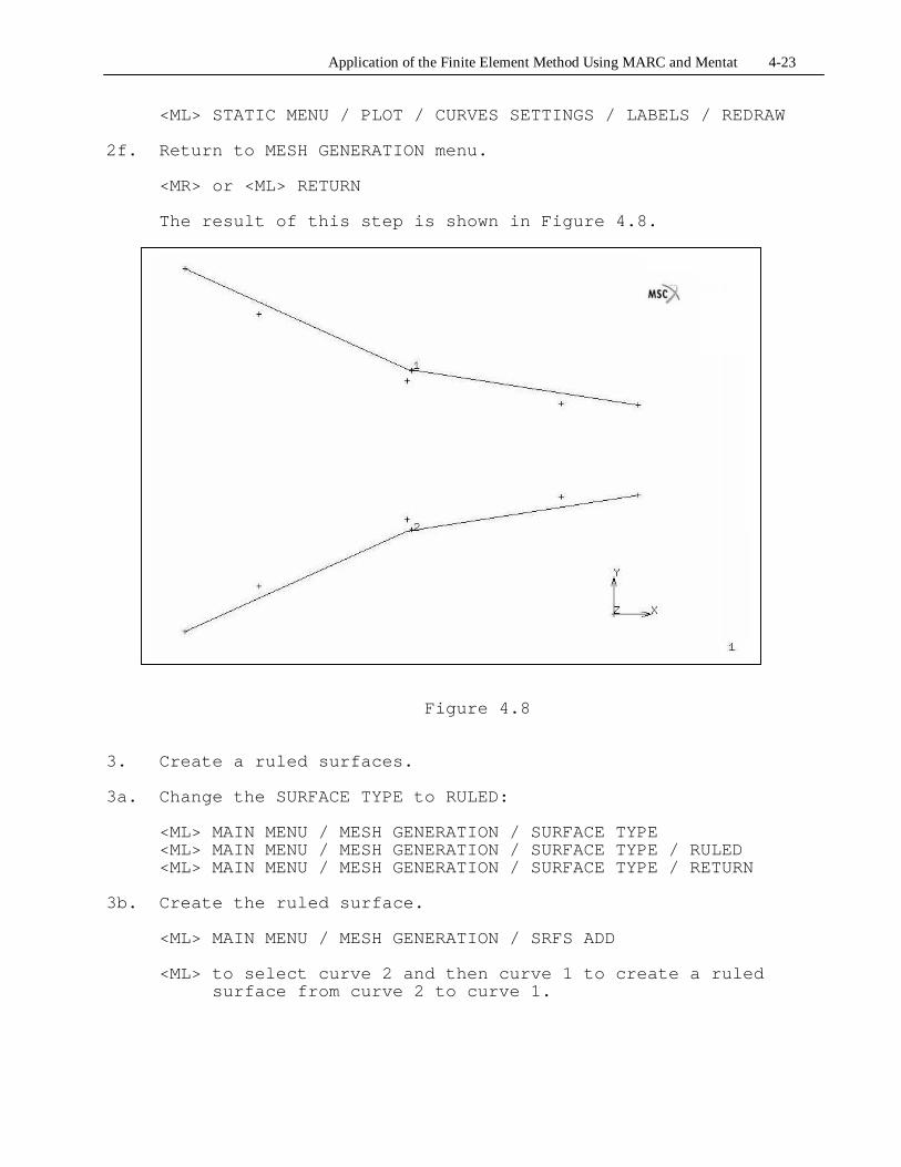
<ML> STATIC MENU / PLOT / CURVES SETTINGS / LABELS / REDRAW 2f. Return to MESH GENERATION menu.
<MR> or <ML> RETURN
The result of this step is shown in Figure 4.8.
Figure 4.8
3. Create a ruled surfaces. 3a. Change the SURFACE TYPE to RULED:
<ML> MAIN MENU / MESH GENERATION / SURFACE TYPE <ML> MAIN MENU / MESH GENERATION / SURFACE TYPE / RULED <ML> MAIN MENU / MESH GENERATION / SURFACE TYPE / RETURN
3b. Create the ruled surface.
<ML> MAIN MENU / MESH GENERATION / SRFS ADD
<ML> to select curve 2 and then curve 1 to create a ruled surface from curve 2 to curve 1.
Application of the Finite Element Method Using MARC and Mentat 4-24
3c. Turn off curve labels.
<ML> STATIC MENU / PLOT <ML> STATIC MENU / PLOT / CURVES SETTINGS <ML> STATIC MENU / PLOT / CURVES SETTINGS / LABELS <ML> STATIC MENU / PLOT / CURVES SETTINGS / LABELS / REDRAW
3d. Return to MESH GENERATION menu.
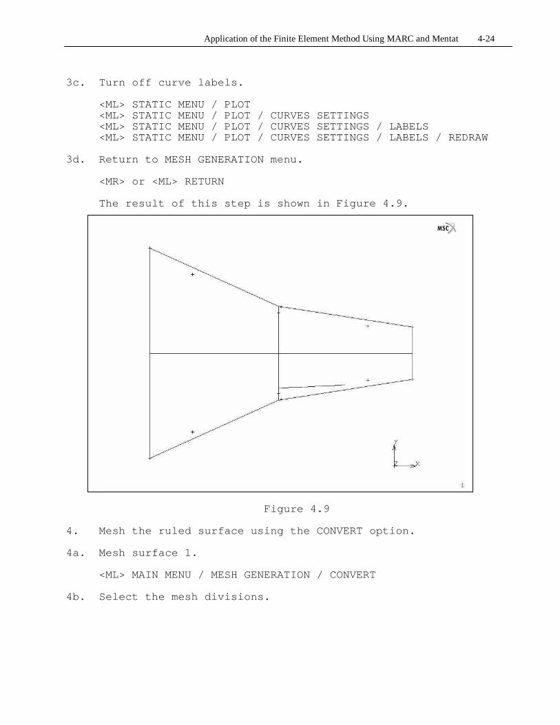
<MR> or <ML> RETURN
The result of this step is shown in Figure 4.9.
Figure 4.9
4. Mesh the ruled surface using the CONVERT option. 4a. Mesh surface 1.
<ML> MAIN MENU / MESH GENERATION / CONVERT 4b. Select the mesh divisions.
Application of the Finite Element Method Using MARC and Mentat 4-25
<ML> MAIN MENU / MESH GENERATION / CONVERT / DIVISIONS
Enter the mesh divisions at the command line, with a space separating each value.
> 30 16
4b. Select the mesh bias factors.
<ML> MAIN MENU / MESH GENERATION / CONVERT / BIAS FACTORS
Enter the mesh bias factors at the command line, with a space separating each value.
> 0.0 0.0
4c. Mesh the surface.
<ML> MAIN MENU / MESH GENERATION / CONVERT / SURFACES TO ELEMENTS
<ML> to select surface 1 (the only surface). <MR> or END LIST
4d. Turn off surface displays.
<ML> STATIC MENU / PLOT <ML> STATIC MENU / PLOT / SURFACES SETTINGS <ML> STATIC MENU / PLOT / SURFACES SETTINGS / SURFACES <ML> STATIC MENU / PLOT / SURFACES SETTINGS / REDRAW
4e. Turn off point displays.
<ML> STATIC MENU / PLOT <ML> STATIC MENU / PLOT / POINTS SETTINGS <ML> STATIC MENU / PLOT / POINTS SETTINGS / POINTS <ML> STATIC MENU / PLOT / POINTS SETTINGS / REDRAW
4f. Turn off curve displays.
<ML> STATIC MENU / PLOT <ML> STATIC MENU / PLOT / CURVES SETTINGS <ML> STATIC MENU / PLOT / CURVES SETTINGS / CURVES <ML> STATIC MENU / PLOT / CURVES SETTINGS / REDRAW
4g. Exit the PLOT menu.
<MR> or <ML> RETURN 4h. Return to MESH GENERATION menu.
Application of the Finite Element Method Using MARC and Mentat 4-26
<MR> or <ML> RETURN
5. Sweep the mesh to insure that all elements are properly
connected.
<ML> MAIN MENU / MESH GENERATION / SWEEP <ML> MAIN MENU / MESH GENERATION / SWEEP / ALL
Note: Duplicate geometrical and mesh entities will be deleted so that proper mesh connectivity is achieved.
Return to MESH GENERATION menu.
<MR> or <ML> RETURN
6. Check for upside down elements.
<ML> MAIN MENU / MESH GENERATION / CHECK <ML> MAIN MENU / MESH GENERATION / CHECK / UPSIDE DOWN
Note: All elements should be numbered locally in a counter-clockwise direction. Those elements numbered locally in a clockwise fashion are defined as upside down, and are highlighted when the above command is issued. These elements should be flipped by executing the FLIP ELEMENTS command.
If the procedure has been followed accurately to this point, the number of upside down elements should be zero. If so, then proceed to step 7. If not, then do the following to flip the elements.
<ML> MAIN MENU / MESH GENERATION / CHECK / FLIP ELEMENTS
Note: The upside down elements are already selected.
<ML> MAIN MENU / MESH GENERATION / CHECK / ALL: SELECT.
Note: Verify that all elements are now oriented correctly.
<ML> MAIN MENU / MESH GENERATION / CHECK / UPSIDE DOWN
Return to the MAIN menu.
<ML> MAIN MENU / MESH GENERATION / CHECK / MAIN
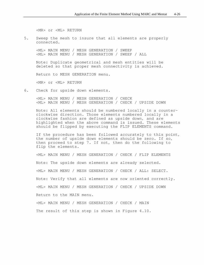
The result of this step is shown in Figure 4.10.
Application of the Finite Element Method Using MARC and Mentat 4-27
Figure 4.10
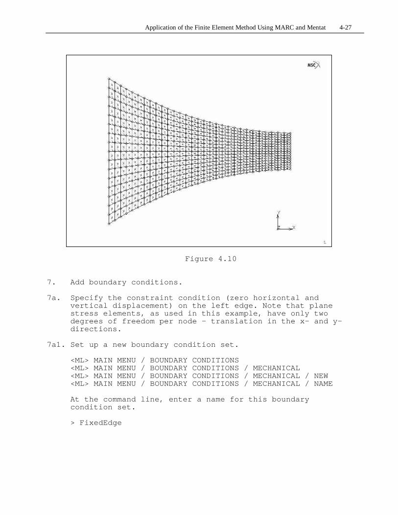
7. Add boundary conditions. 7a. Specify the constraint condition (zero horizontal and
vertical displacement) on the left edge. Note that plane stress elements, as used in this example, have only two degrees of freedom per node – translation in the x- and y-directions.
7a1. Set up a new boundary condition set.
<ML> MAIN MENU / BOUNDARY CONDITIONS <ML> MAIN MENU / BOUNDARY CONDITIONS / MECHANICAL <ML> MAIN MENU / BOUNDARY CONDITIONS / MECHANICAL / NEW <ML> MAIN MENU / BOUNDARY CONDITIONS / MECHANICAL / NAME
At the command line, enter a name for this boundary condition set.
> FixedEdge
Application of the Finite Element Method Using MARC and Mentat 4-28
7a2. Define the nature of the boundary condition.
<ML> MAIN MENU / BOUNDARY CONDITIONS / MECHANICAL / FIXED DISPLACEMENT
<ML> MAIN MENU / BOUNDARY CONDITIONS / MECHANICAL / FIXED DISPLACEMENT / DISPLACEMENT X
<ML> MAIN MENU / BOUNDARY CONDITIONS / MECHANICAL / FIXED DISPLACEMENT / DISPLACEMENT Y
The small box to the immediate left of the button for DISPLACEMENT X and DISPLACEMENT Y should now be highlighted.
<ML> MAIN MENU / BOUNDARY CONDITIONS / MECHANICAL /
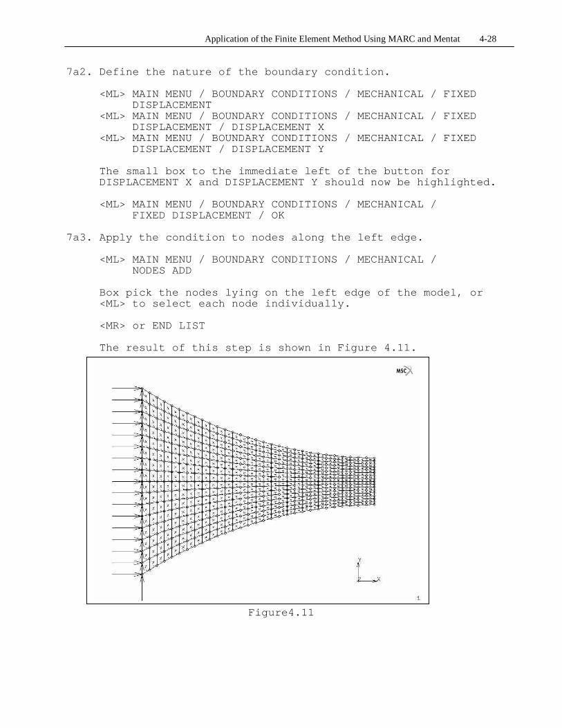
FIXED DISPLACEMENT / OK 7a3. Apply the condition to nodes along the left edge.
<ML> MAIN MENU / BOUNDARY CONDITIONS / MECHANICAL / NODES ADD
Box pick the nodes lying on the left edge of the model, or <ML> to select each node individually. <MR> or END LIST The result of this step is shown in Figure 4.11.
Figure4.11

Application of the Finite Element Method Using MARC and Mentat 4-29
7b. Specify the vertical point load on the right edge of the model.
It will be assumed that the load is applied to a single node
located at the center of the right edge of the model. This type of load is specified as a point load.
7b1. Set up a new boundary condition set.
<ML> MAIN MENU / BOUNDARY CONDITIONS <ML> MAIN MENU / BOUNDARY CONDITIONS / MECHANICAL <ML> MAIN MENU / BOUNDARY CONDITIONS / MECHANICAL / NEW <ML> MAIN MENU / BOUNDARY CONDITIONS / MECHANICAL / NAME
At the command line, enter a name for this boundary condition set.
> VerticalLoad
7b2. Define the nature of the boundary condition.
<ML> MAIN MENU / BOUNDARY CONDITIONS / MECHANICAL / POINT LOAD
<ML> MAIN MENU / BOUNDARY CONDITIONS / MECHANICAL / POINT LOAD / FORCE Y
The small box to the immediate left of the button for FORCE Y should now be highlighted.
7b3. Define the magnitude of the load by entering the value at
the command prompt.
> 1.0e4
<ML> MAIN MENU / BOUNDARY CONDITIONS / MECHANICAL / POINT LOAD / OK
7b4. Apply the condition to the center node on the right edge of
the model.
<ML> MAIN MENU / BOUNDARY CONDITIONS / MECHANICAL / NODES ADD
<ML> pick the center node on the right edge of the model.
<MR> or END LIST
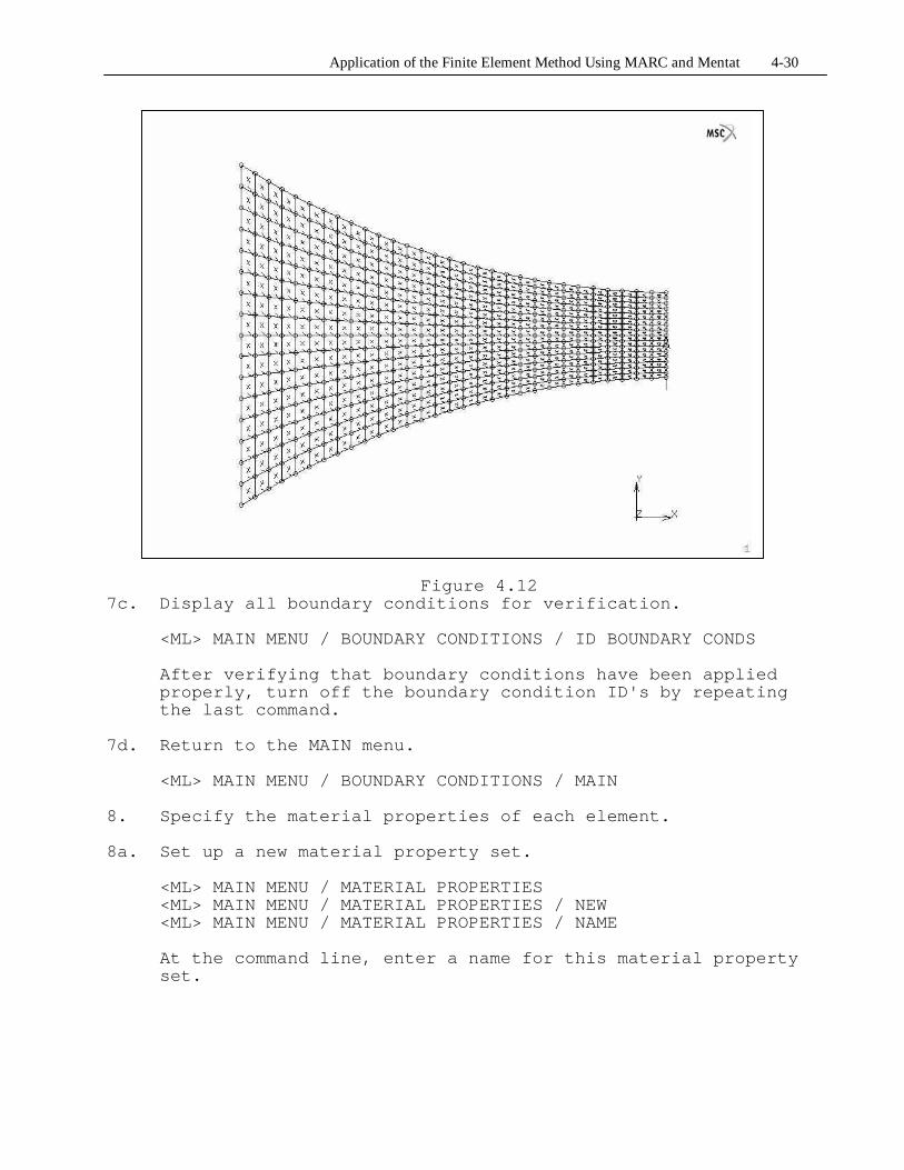
The result of this step is shown in Figure 4.12.
Application of the Finite Element Method Using MARC and Mentat 4-30
Figure 4.12
7c. Display all boundary conditions for verification.
<ML> MAIN MENU / BOUNDARY CONDITIONS / ID BOUNDARY CONDS
After verifying that boundary conditions have been applied properly, turn off the boundary condition ID's by repeating the last command.
7d. Return to the MAIN menu.
<ML> MAIN MENU / BOUNDARY CONDITIONS / MAIN 8. Specify the material properties of each element. 8a. Set up a new material property set.
<ML> MAIN MENU / MATERIAL PROPERTIES <ML> MAIN MENU / MATERIAL PROPERTIES / NEW <ML> MAIN MENU / MATERIAL PROPERTIES / NAME
At the command line, enter a name for this material property set.
Application of the Finite Element Method Using MARC and Mentat 4-31
> Steel 8b. Define the nature of the material.
<ML> MAIN MENU / MATERIAL PROPERTIES / ISOTROPIC <ML> MAIN MENU / MATERIAL PROPERTIES / ISOTROPIC /
YOUNG'S MODULUS
> 29.0e6
<ML> MAIN MENU / MATERIAL PROPERTIES / ISOTROPIC / POISSON'S RATIO
> 0.30
Note: Only Young's modulus and Poisson's ratio need to be specified for this problem.
<ML> MAIN MENU / MATERIAL PROPERTIES / ISOTROPIC / OK
8c. Apply the material properties to all elements.
<ML> MAIN MENU / MATERIAL PROPERTIES / ELEMENTS ADD
Since the properties are being applied to all elements in the model, the simplest way to select the elements is to use the ALL EXISTING option.
<ML> ALL: EXIST.
8d. Display all material properties for verification.
<ML> MAIN MENU / MATERIAL PROPERTIES / ID MATERIALS
After verifying that material properties have been applied properly, turn off the material property ID's by repeating the last command.
8e. Return to the MAIN menu.
<ML> MAIN MENU / MATERIAL PROPERTIES / MAIN 9. Specify the thickness of each element. 9a. Set up a new geometric property set.
<ML> MAIN MENU / GEOMETRIC PROPERTIES <ML> MAIN MENU / GEOMETRIC PROPERTIES / NEW <ML> MAIN MENU / GEOMETRIC PROPERTIES / NAME

Application of the Finite Element Method Using MARC and Mentat 4-32
At the command line, enter a name for this geometric property set.
> Thickness
9b. Define the nature of the geometric property.
<ML> MAIN MENU / GEOMETRIC PROPERTIES / PLANAR <ML> MAIN MENU / GEOMETRIC PROPERTIES / PLANAR /
PLANE STRESS <ML> MAIN MENU / GEOMETRIC PROPERTIES / PLANAR /
PLANE STRESS / THICKNESS
> 1.0
<ML> MAIN MENU / GEOMETRIC PROPERTIES / PLANAR / PLANE STRESS / OK
9c. Apply the geometric property to all elements.
<ML> MAIN MENU / GEOMETRIC PROPERTIES / PLANAR / ELEMENTS ADD
Since the property is being applied to all elements in the model, the simplest way to select the elements is to use the ALL EXISTING option.
<ML> ALL: EXIST.
9d. Display all geometric properties for verification.
<ML> MAIN MENU / GEOMETRIC PROPERTIES / ID GEOMETRIES
After verifying that geometric properties have been applied properly, turn off the geometric property ID's by repeating the last command.
9e. Return to the MAIN menu.
<ML> MAIN MENU / GEOMETRIC PROPERTIES / MAIN 10. Prepare the loadcase.
<ML> MAIN MENU / LOADCASES <ML> MAIN MENU / LOADCASES / MECHANICAL <ML> MAIN MENU / LOADCASES / MECHANICAL / STATIC <ML> MAIN MENU / LOADCASES / MECHANICAL / STATIC / LOADS
Verify that all loads (i.e., boundary constraints and point load) created in step 7 are selected. The small box to the
Application of the Finite Element Method Using MARC and Mentat 4-33
immediate left of all selected loads will be highlighted. If they are not already selected, then select them using the <ML>.
<ML> MAIN MENU / LOADCASES / MECHANICAL / STATIC /
LOADS / OK <ML> MAIN MENU / LOADCASES / MECHANICAL / STATIC / OK <ML> MAIN MENU / LOADCASES / MECHANICAL / MAIN
11. Prepare the job for execution. 11a. Specify the analysis class and select loadcases.
<ML> MAIN MENU / JOBS <ML> MAIN MENU / JOBS / MECHANICAL <ML> MAIN MENU / JOBS / MECHANICAL / lcase1
11b. Select the analysis dimension.
<ML> MAIN MENU / JOBS / MECHANICAL / PLANE STRESS 11c. Select the desired output variables.
<ML> MAIN MENU / JOBS / MECHANICAL / JOB RESULTS <ML> MAIN MENU / JOBS / MECHANICAL / JOB RESULTS / Stress <ML> MAIN MENU / JOBS / MECHANICAL / JOB RESULTS /
Equivalent Von Mises Stress <ML> MAIN MENU / JOBS / MECHANICAL / JOB RESULTS / OK
<ML> MAIN MENU / JOBS / MECHANICAL / OK
11d. Select the element to use in the analysis.
<ML> MAIN MENU / JOBS / ELEMENT TYPES <ML> MAIN MENU / JOBS / ELEMENT TYPES / MECHANICAL <ML> MAIN MENU / JOBS / ELEMENT TYPES / MECHANICAL /
PLANE STRESS
Select element number 3, a fully-integrated, four-noded quadrilateral.
<ML> MAIN MENU / JOBS / ELEMENT TYPES / MECHANICAL /
PLANE STRESS / 3 <ML> MAIN MENU / JOBS / ELEMENT TYPES / MECHANICAL /
PLANE STRESS / OK 11e. Apply the element selection to all elements.

Application of the Finite Element Method Using MARC and Mentat 4-34
Since the element type is being applied to all elements in the model, the simplest way to select the elements is to use the ALL EXISTING option.
<ML> ALL: EXIST.
11f. Display all element types for verification.
<ML> MAIN MENU / JOBS / ELEMENT TYPES / ID TYPES
After verifying that element types have been applied properly, turn off the element type ID's by repeating the last command.
<ML> MAIN MENU / JOBS / ELEMENT TYPES / RETURN
11g. SAVE THE MODEL!
<ML> STATIC MENU / FILES <ML> STATIC MENU / FILES / SAVE AS
In the box to the right side of the SELECTION heading, type in the name of the file that you want to create. The name should be of the form FILENAME.mud, where FILENAME is a name that you choose.
<ML> STATIC MENU / FILES / SAVE AS / OK <ML> STATIC MENU / FILES / RETURN
11h. Execute the analysis.
<ML> MAIN MENU / JOBS / RUN <ML> MAIN MENU / JOBS / RUN / SUBMIT 1
11i. Monitor the status of the job.
<ML> MAIN MENU / JOBS / RUN / MONITOR
When the job has completed, the STATUS will read: Complete. A successful run will have an EXIT NUMBER of 3004. Any other exit number indicates that an error occurred during the analysis, probably due to an error in the model.
<ML> MAIN MENU / JOBS / RUN / OK <ML> MAIN MENU / JOBS / RETURN
12. Postprocess the results. 12a. Open the results file and display the results.

Application of the Finite Element Method Using MARC and Mentat 4-35
<ML> MAIN MENU / RESULTS <ML> MAIN MENU / RESULTS / OPEN DEFAULT <ML> MAIN MENU / RESULTS / CONTOUR BANDS
A contour plot of the X-displacement should appear.
12b. Display a different output variable.
<ML> MAIN MENU / RESULTS / SCALAR <ML> MAIN MENU / RESULTS / SCALAR / Comp 11 of Stress <ML> MAIN MENU / RESULTS / SCALAR / OK
A contour plot of the stress in the X-direction should appear.
12c. Display nodal values of the output variable.
<ML> MAIN MENU / RESULTS / NUMERICS
It is difficult to read the values when the entire model is displayed. To view the nodal values, zoom in on the region of interest using the zoom box on the static menu. To view the entire model again, use the FILL command on the static menu.
12d. Display the deformed shape. <ML> DEF ONLY The deformed shape of the beam should be visible. To
increase or decrease the scaling factor for the deformed shape, select SETTINGS next to the DEFORMED SHAPE heading, then either select AUTOMATIC or increase the FACTOR under the DEFORMATION SCALING heading. Check that the deformed shape seems reasonable (e.g., Does it agree with intuition? Are the boundary conditions satisfied? etc.)