EM 1110-2-1003 1 Jan 02

Chapter 4 Survey Accuracy Estimates for Dredging and Navigation Projects 4-1. General Scope This chapter defines the hydrographic surveying accuracy standards used in Table 3-1. It also provides guidance on statistically evaluating the accuracy of an observed geospatial point (i.e., a depth measurement) or a set of points in a database. Such evaluations are used in assessing the accuracy of a hydrographic survey relative to channel clearance, dredge measurement and payment, and related coastal engineering or hydraulic engineering computations. 4-2. Hydrographic Survey Accuracy Hydrographic surveying is, in its most basic form, a two-legged, open-end traverse. The first leg of the traverse is the positioning of the survey platform. The X-Y location of the survey boat is typically determined by visual or electronic methods described in this manual. The elevation of the boat is usually obtained relative to the elevation of the local water surface. Thus the vessel position and elevation are independent measurements—each with their own accuracies. The underwater depth measurement—the second leg of the open-end traverse--is made relative to the water surface using mechanical or acoustic methods. Depth measurement methods have widely varying accuracies. Unlike conventional terrestrial surveying, there is no method to “close out” the traverse on a measured depth. Therefore, the accuracy assessment of an observed depth can only be estimated using statistical assumptions. In addition, hydrographic surveying has few real-time quality control indicators to verify or check its resultant accuracy. Since the subsurface point is not visible, even gross blunders are difficult to detect. Maintaining prescribed accuracy criteria, therefore, requires precision, care, and quality control in the measurement process. There are few opportunities to correct or adjust the data after the fact. a. Vessel horizontal position accuracy. A survey vessel's horizontal position is determined by an open-ended survey method--trilateration, triangulation, or traverse. Because these positioning methods have no independent check, the accuracy of an offshore position is totally dependent on the precision of the measuring process. The positional accuracy is a function of the measurement method, distance from the reference baseline, atmospheric conditions, sea state, and numerous other factors. Positional accuracies can vary from less than 0.5 meters (carrier phase real-time-kinematic (RTK) DGPS) to over 20 meters when visual location methods are used.

b. Depth measurement accuracy. Depth measurement accuracy likewise has many potential error components. These include measurement method (mechanical or acoustic), sea state, water temperature and salinity, transducer beam width, bottom irregularity, bottom consistency, and vessel heave-pitch-roll motions. In addition, the depth must be referenced to the local water surface which, in turn, must be referenced to a datum plane at some remote point. All these factors make up the error budget of the depth measurement.

c. Combined horizontal and vertical accuracy. The overall accuracy of an observed bottom depth elevation is dependent on many random and systematic errors that are present in the measurement processes used to measure that elevation. This makes any quantitative comparisons of the observed elevations difficult, particularly in areas of irregular terrain. Thus, any efforts to compare different surveys made over the same presumed point must factor in the inaccuracies in all three dimensions and their resultant impact on an existing terrain gradient. An overall assessment of the accuracy of an individual depth or bottom elevation must also fully consider all the error components contained in the observations that were used to determine the point. The resultant accuracy of a single depth point is represented by a 3-D error ellipsoid, as shown in Figure 4-1. The dimensions of this ellipsoid are indicated by the standard errors in all three dimensions—sX, sY, and sZ. The size and orientation of this 3-D ellipsoid is determined from all the various

4-1

EM 1110-2-1003 1 Jan 02 error components (“uncertainties”) that made up the position and depth measurements. In general, the dimensions of the ellipsoid are larger in the X and Y planes, due to positional accuracy being less accurate than the depth measurement (e.g., 2 meter DGPS accuracy and +1 foot depth accuracy).

TransducerTransducer elevationWater surface elevation

Positioning system

Measured depth

Depth error ellipsoidSX

SZ

SY

Positional uncertainty ellipse

Depth measurement uncertainty

Figure 4-1. Three-dimensional uncertainty of a measured depth d. The accuracy of hydrographic survey measurements is therefore highly dependent on the accuracy of each measurement component, including calibrations, parametric correlation (time, distance, or velocity) of the measured components, reductions, and corrections made to the data. It is also highly time-dependent, given the inability to make frequent calibrations, short-term physical changes in the measurement mediums (water and air), and the wide area over which these variations may occur. Hydrographic surveys can exhibit different results when measurements are repeated at different times. This variation becomes obvious when comparing cross sections (and resultant end area volumes) measured by different survey crews and/or systems, or even the same crew and system in many cases. It is extremely difficult to independently verify the accuracy of a dynamic hydrographic measurement. In general, the accuracy of a hydrographic survey can only be estimated based on results obtained during repeated equipment calibrations. Since these calibrations are not always performed in a dynamic (on-line) environment, the ultimate accuracy must be estimated (thus the use of the term “estimated accuracy”) using statistical estimating measures. Other techniques that may be used to evaluate the accuracy of a hydrographic survey include cross-check lines and performance tests in multibeam surveys. These are described in later chapters of this manual. 4-3. Accuracy, Precision, and Root Mean Square Error A clear distinction must be made between the terms accuracy and precision when referring to a hydrographic measurement or series of measurements (i.e., a data set from a particular survey). These concepts are illustrated in the depth observation dispersion curves in Figure 4-2. In this figure, observed depths are dispersed around a "true" value that is unknown. The depth observations contain both random errors and systematic biases. Biases are often referred to as systematic or external errors and may contain observational blunders. A constant error in tide or stage would be an example of a bias. Random errors are those errors present in the measurement system that cannot be easily minimized by further calibration.

4-2

EM 1110-2-1003 1 Jan 02

Examples include echo sounder resolution, water sound velocity variations, tide/staff gage reading resolution, etc. The precision of the observations is a measure of the closeness of a set of measurements--or their internal agreement-- shown as σ RANDOM ERROR in the figure. This is synonymous with “repeatability.” Accuracy relates to the closeness of measurements to their true or actual value. Accuracy, therefore, includes both precision (σ RANDOM ERROR) and any systematic biases (shown as σ BIAS ) that may be present. For example, a depth digitizer may repeatedly display a given depth to precisely + 0.1 ft; however, the accuracy of the depth may be only + 1.5 ft when other error components are included. Repeated observations during a static calibration will not always remove systematic biases that may be present--e.g., a tidal datum error in a depth observation. High precision, or repeatability, does not necessarily indicate high accuracy. Apparently scattered data may be highly accurate, whereas highly repeatable data could have large undetected biases.

a. The upper curve in Figure 4-2 illustrates such a case. The measurements have a high "precision" of say + 0.2 ft but there could be a (-) 1.3 ft bias due to a tidal modeling error at the work site, a bar check calibration blunder, or erroneous squat/settlement correction. A smooth, flat bottom in calm waters would yield a small variance such as the + 0.2 ft value.

b. The lower curve is an example of a low "precision" depth measurement. In this case, the depth

observations vary by say + 0.8 ft (σ RANDOM ERROR) but there is only a small (+) 0.1 ft bias in the observations. The random error component could be due to such causes as uneven bottom topography, bottom vegetation, positioning error, or speed of sound variations in the water column--errors that are difficult or impossible to remove by calibration. The small (+) 0.1 ft bias indicates that most systematic errors have been removed.

c. Both curves shown in Figure 4-2 occur in real hydrographic survey data sets. The preferred distribution is the lower curve in that the systematic bias is minimal. A degree of randomness in the observations is far more tolerable than systematic bias errors. Thus the objective is to minimize the biases in a survey. Biases can be estimated using cross-line checks or multibeam performance tests.

+0.2 ft

Bias (-) 1.3 ft

+0.8 ft

Bias (+) 0.1 ft

P= 68%

P= 68%

RMS = ( 0.2 2 + 1.3 2 ) 1/2 = + 1.3 ft

RMS = ( 0.8 2 + 0.1 2 ) 1/2 = + 0.8 ft

Figure 4-2. Typical dispersion curves for depth observations

4-3

EM 1110-2-1003 1 Jan 02

d. Root Mean Square error measure. Given geospatial depth observations containing both random errors and systematic biases, a consistent accuracy measurement is required. These biases and random errors can be combined to obtain the Mean Square Error (MSE) or Root Mean Square (RMS) error of a depth observation. The equation for computing one-dimensional MSE or RMS error is:

RMS error = sqrt [ σ 2RANDOM ERROR + σ 2BIAS ] (Eq 4-1)

The RMS error estimator is used for comparing relative accuracies of estimates that differ substantially in bias and precision. The random error and bias components in Equation 4-1 can be estimated from actual depth comparisons--either relative to a fixed "true" surface (e.g., lock chamber) or based on duplicate measurements over the same terrain.

(1) The distribution curve shown in Figure 4-2 could represent repeated depth measurements taken over some "true" point--say observations made in a regulated lock chamber where the depth is accurately known and controlled. In practice, such a "true" (or known) elevation in a lock chamber is rarely ever available, and depth accuracies must be estimated using comparative readings taken over the same point on the bottom (i.e., cross-line checks or performance tests). If the depth observations are randomly distributed, the mean of all the observations will fall at the peak of the distribution curve. The mean of a sample series of n depth measurements x is computed by:

Mean depth z M = Σ [ z i ] / ( n ) (Eq 4-2)

where n = number of observed depths in sample z i = individual observed depths (i = 1 to i = n) The difference of the mean z M from the "true" depth (shown as σ BIAS in Figure 4-2) represents a systematic error in the observations that was not removed by calibration or modeling. The precision to which the mean is computed is a function of the number of observation "n." The more observations in the sample, the more precisely the mean can be determined. Some biases are difficult to identify or remove. Examples of this type of bias are temperature change, salinity changes, and tidal modeling. These biases are systematic in nature but will vary randomly in time and position. They may be considered random from survey to survey, and this allows their error contribution to be estimated with statistics.

(2) The shape, or spread, of the bell-shaped error distribution curve is an indicator of the dispersion in the depth observations--i.e., the random errors. The upper curve in Figure 4-2 indicates tightly packed observations and the lower curve indicates high variability in the observations. If the depth errors are assumed to be random, then the dispersion of the depth observations can be estimated by computing the Standard Error ( s Z ) of the sample: Standard error s Z = sqrt [ ( 1 / (n - 1)) Σ [ z i - z M ] 2 ]

(Eq 4-3) The magnitude of the dispersion is shown as σ RANDOM ERROR in Figure 4-2. This distance represents the + one-sigma (1-σ) points on the normal distribution curve, with the cross-hatched area being a probability of 68% that the computed mean of the observed depths falls within this area of the curve. For example, on the lower curve, 68% of observed depths would fall within + 0.8 ft from the mean. This means that a hydrographic survey data set containing hundreds or thousands of geospatial points has a dispersion of + 0.8 ft at the 1-σ (68%) level. 32% of the depths can be expected to fall outside the + 0.8 ft interval. Which individual depths are inside or outside this interval cannot be determined--only that the estimated 1-σ standard deviation of the survey is + 0.8 ft. The overall RMS accuracy may be larger if biases are present in the data.

4-4

EM 1110-2-1003 1 Jan 02

(3) The RMS error is estimated by substituting the standard (random) error (Equation 4-3) and bias (Equation 4-2) into Equation 4-1. This is illustrated in Figure 4-2.

e. RMS error should not exceed the stated tolerance in Table 3-1 for a USACE survey class. Minimization of the many random and systematic errors (and blunders) present in horizontal and vertical measurements is accomplished by repeated instrument calibration, adherence to prescribed procedural criteria, and recognition of limitations in the measurement equipment. Careful field procedures, coupled with adequate survey planning, equipment selection, and equipment maintenance, are also essential. f. Subsequent chapters in this manual discuss some of the more common error sources in hydrographic surveys. These factors apply to manual hydrographic survey methods or those using electronic positioning and to echo sounding depth measurement systems. All these factors are capable of producing errors that behave systematically, resulting in biases in a given survey. One objective of the criteria presented in this manual is to reduce the magnitudes of these errors to tolerable levels and then presume that they will offset one another randomly (noise like), with the resultant horizontal and vertical standard errors falling within the prescribed levels for each survey class. 4-4. One-Dimensional Depth Accuracy Estimates--95% Confidence Estimation Level RMS depth errors are computed and reported at the 95% confidence level in accordance with FGDC Geospatial Positioning Accuracy Standards (Parts 1 and 3)--see Appendix A. USACE depth accuracy tolerances in Table 3-1 are expressed at this 95% confidence level. This simply means that on average 19 of every 20 observed depths will fall within the specified accuracy tolerance. Since the 1-sigma (68%) standard is computed when depth accuracy is assessed, it can be converted to a 95% RMS confidence level statistic by the following: RMS (95%) depth accuracy = 1.96 · RMS (68%)

(Eq 4-4)

a. The above formula assumes the data are random and contain no large biases. It represents the area under the +1.96-σ points on the distribution curves in Figure 4-2. This area covers 95% probable error of all points in a data set. For example, when a data set for a pre-dredge survey of a 45-ft project is reported accurate to + 2.0 ft, this means that 95% of the points in the data set will have an error with respect to true ground position that is equal to or smaller than the reported accuracy value. 5% of the depths in the data set will have errors exceeding + 2.0 ft. Again, it is impossible to determine which particular depth in the data base lies within or outside the stated accuracy tolerance. If the pre-dredge survey was performed using multibeam equipment, and 100,000 points are in a binned grid, some 5, 000 of these points could be outside the 95% tolerance level. For this reason, a single depth observation above a required grade cannot be assumed to be representative of the area—multiple observations above grade are needed to statistically defend any assessment. Unlike land-based topographic and photogrammetric surveys, it is extremely difficult to independently determine the resultant accuracy of any hydrographic survey. Photogrammetric or topographic survey elevation accuracies are assessed by comparing observed elevations with those determined by a “significantly” more accurate method—e.g., a photo-derived elevation point is tested against that obtained by a spirit level or total station. Typically 20 or more points are tested and if 19 of 20 fall within the required tolerance, then the survey is deemed to be within the required accuracy. Hydrographic surveys do not have “significantly” more accurate independent method of testing observed data. Most depth measurement methods contain inherent errors of such magnitude that it is difficult to statistically certify one method as more accurate than the other. One exception might be testing observed depths inside a lock chamber. b. Confidence of accuracy estimates. Confidence intervals are used to provide an indication of how good an accuracy estimate is and how much it can be relied on (Mikhail, 1976). Confidence intervals are

4-5

EM 1110-2-1003 1 Jan 02 also termed degree of confidence. The confidence interval describes a boundary within which there is a probability that the computed mean (or standard error) of depths in a data set fall relative to the true or actual mean value (which is not known). The larger the observed data set, the better is the confidence of a computed mean or standard error. Confidence intervals of means or standard deviations are also expressed at the 95% level. The confidence interval of the mean has also been termed the standard error of the mean.

(1) For example, assume 50 depth comparisons are made between cross-line intersections from two overlapping surveys conducted on different days. Average water depth was 45 ft. The bias between the two surveys was (-) 0.02 ft--i.e., negligible. The computed standard deviation for the 50 points was + 0.85 ft. The 95% confidence interval of the computed mean (+ 0.24 feet) is computed by standard t-distribution statistical methods.

+ (t 0.025) (s) / ( n ) 1/2 = +2.01 · 0.85 / (50) 1/2 = +0.24 ft

where t = t-test critical value from Student-t probability table with (50-1) degrees of freedom and

0.025 probability s = computed standard deviation of the sample n = number of data values in sample The 95% confidence interval of the computed mean is then shown as: Probability { (-) 0.26 < computed mean (- 0.02 ft) < (+) 0.22 } = 0.95 (95%) This means that the computed mean (-0.02 ft) is uncertain up to + 0.24 ft at the 95% confidence level. It also means that a sufficient number of comparisons must be made in order to assess the accuracy of a survey. If it is required to achieve a + 0.2 ft confidence in the mean to preclude against the existence of systematic biases, then more comparison points than 50 are needed. Had 100 cross-line comparisons been conducted, then the confidence interval of the computed mean would be + 0.17 ft, and the confidence range shown as: Probability { (-) 0.19 < computed mean (-0.02) < (+) 0.15 } = 0.95 (95%) With 100 comparisons, the + 0.17 estimated confidence of the mean is below the desired +0.20. To achieve a more reliable (or confident) estimate of the mean requires considerably more data set comparisons. Better accuracies are also achieved with smaller standard deviations in the data.

(2) Minimizing biases by assessing the standard error of the mean is critical for hydrographic surveys involving payment. Any constant bias present in a survey must be evaluated and reduced. Corps QA Performance Tests allow a difference (or tolerance) of up to 0.2 feet when two surveys of the same area are compared--see Performance Test standards in Tables 3-1, 9-1, 10-1, and 11-2. However, a much smaller mean difference is desired in practice. To ensure that the standard error of the mean does not exceed, say a + 0.05 ft level, then the number of comparisons can be computed given the assumed survey's 1-σ RMS error (function of project depth). If a survey is performed in 50-ft of water (i.e., required RMS accuracy = + 2.0 ft), and a +0.05 ft confidence in the mean is desired, then, at minimum, some 1,500 cross-line or multibeam comparison points are needed. This number of comparisons would only be practical for multiple transducer or multibeam surveys. (3) The 95% confidence of the computed standard deviation can also be estimated using statistical methods--see Mikhail, 1976.

4-6

EM 1110-2-1003 1 Jan 02

4-5. Depth Measurement Error Components Major error components of electronic echo sounding depth measurement methods are described in the following paragraphs. From these error sources, relative accuracy estimates for varying project conditions can be derived. The criteria standards for depths in Table 3-1 were established from these estimates. a. Depth measurement system. The precision of any depth measurement will, in general, degrade as a function of water depth. The accuracy of an echo-sounding measurement degrades with depth due to a number of electronic and physical factors inherent in the sound travel-time measurement process, i.e., changes in water temperature, salinity, etc. Multibeam depth measurement accuracy typically degrades over the outer beams on the array, depending on the type of depth resolution method employed and the bottom characteristics or reflectivity. Beam refraction (ray bending) can also be a problem if not corrected. Older analog recording devices have mechanical movements that contribute to inaccuracies in the recorded depth. These errors are minimized by frequent calibration of the echo sounding equipment. b. System calibration and alignment. Calibration of electronic echo sounding instruments is, in itself, an imprecise process, particularly in deep-draft projects. Because bar check calibrations are performed while the vessel is stationary, actual dynamic survey conditions are not truly simulated. The bar check procedure is not error-free due to line slope in currents, signal strength variations between the bar plate and the typical bottom condition, loading changes during calibration, and other factors. The accuracy of a bar check calibration ranges from +0.1 to +0.2 ft, depending on the depth of the bar and sea conditions. On small boats, personnel movement during bar checks may vary the transducer draft from that under normal running conditions, causing a constant index error to occur. Velocity probes are in themselves dependent on the accuracy and stability of their initial reference calibrations. Calibration of multibeam swath systems is especially critical. Repeatability of some patch tests is difficult to achieve, due to inadequate vessel position and terrain factors. c. Resolution of measured elevations. An accuracy of less than 0.1 ft is not possible on mechanical recording echo sounders with relatively small-scale vertical divisions. Electronic depth digitizing devices typically record and log depth data to a precision (not accuracy) of +0.1 ft. d. Echo sounding system draft/index errors. Echo sounding measurements made from a hull- or side-mounted transducer must be corrected for the distance between the transducer and the reference water surface. This distance is normally referred to as the “draft” correction. Due to mechanical and electrical indexing errors present in an echo sounding device, this “draft” correction is not always equal to the physical (as-measured) distance between the water surface and transducer plate. Thus, the so-called “draft” setting on an echo sounder should not be arbitrarily adjusted based only on short-term physical measurements of the vessel's draft. Only a bar check calibration will effectively confirm this distance or confirm that it is stable over the long term. Subsequent loading changes during the survey (added personnel, fuel, etc.) may be adjusted for based on differential changes to a vessel's draft. The adequacy of such adjustments should have been confirmed by a bar check calibration. Errors due to inadequate compensation for the varied index, loading, and draft variations are systematic and can be significant, especially on small boats with side-mounted transducers. These errors can exceed 0.5 ft in some instances. e. Vertical reference datum. Hydrographic depth measurements are reduced and referenced to the local water surface at the time the measurement is made. This water surface is normally referenced to an on-shore reference benchmark or gage. The accuracy of the entire process is highly variable, and systematic errors in the survey can result if adequate precautions are not taken. The most significant error component involves the assumed stability of the water surface between the on-shore gage and the survey vessel. This stability is usually valid in most non-tidal lakes, impoundment reservoirs, and rivers where extensive stage surface modeling has been performed, and staff gages can be set at every 0.2- to 0.4-ft change in river slope. In these areas, interpolated vertical reference accuracies within +0.1 ft are attainable. However, on coastal navigation projects subject to tidal influences, any surface gradients between the gage and underway vessel

4-7

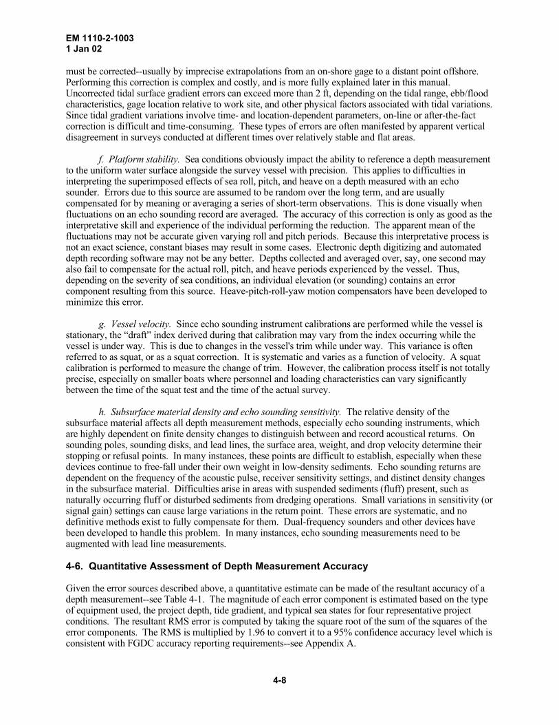
EM 1110-2-1003 1 Jan 02 must be corrected--usually by imprecise extrapolations from an on-shore gage to a distant point offshore. Performing this correction is complex and costly, and is more fully explained later in this manual. Uncorrected tidal surface gradient errors can exceed more than 2 ft, depending on the tidal range, ebb/flood characteristics, gage location relative to work site, and other physical factors associated with tidal variations. Since tidal gradient variations involve time- and location-dependent parameters, on-line or after-the-fact correction is difficult and time-consuming. These types of errors are often manifested by apparent vertical disagreement in surveys conducted at different times over relatively stable and flat areas. f. Platform stability. Sea conditions obviously impact the ability to reference a depth measurement to the uniform water surface alongside the survey vessel with precision. This applies to difficulties in interpreting the superimposed effects of sea roll, pitch, and heave on a depth measured with an echo sounder. Errors due to this source are assumed to be random over the long term, and are usually compensated for by meaning or averaging a series of short-term observations. This is done visually when fluctuations on an echo sounding record are averaged. The accuracy of this correction is only as good as the interpretative skill and experience of the individual performing the reduction. The apparent mean of the fluctuations may not be accurate given varying roll and pitch periods. Because this interpretative process is not an exact science, constant biases may result in some cases. Electronic depth digitizing and automated depth recording software may not be any better. Depths collected and averaged over, say, one second may also fail to compensate for the actual roll, pitch, and heave periods experienced by the vessel. Thus, depending on the severity of sea conditions, an individual elevation (or sounding) contains an error component resulting from this source. Heave-pitch-roll-yaw motion compensators have been developed to minimize this error. g. Vessel velocity. Since echo sounding instrument calibrations are performed while the vessel is stationary, the “draft” index derived during that calibration may vary from the index occurring while the vessel is under way. This is due to changes in the vessel's trim while under way. This variance is often referred to as squat, or as a squat correction. It is systematic and varies as a function of velocity. A squat calibration is performed to measure the change of trim. However, the calibration process itself is not totally precise, especially on smaller boats where personnel and loading characteristics can vary significantly between the time of the squat test and the time of the actual survey.

h. Subsurface material density and echo sounding sensitivity. The relative density of the subsurface material affects all depth measurement methods, especially echo sounding instruments, which are highly dependent on finite density changes to distinguish between and record acoustical returns. On sounding poles, sounding disks, and lead lines, the surface area, weight, and drop velocity determine their stopping or refusal points. In many instances, these points are difficult to establish, especially when these devices continue to free-fall under their own weight in low-density sediments. Echo sounding returns are dependent on the frequency of the acoustic pulse, receiver sensitivity settings, and distinct density changes in the subsurface material. Difficulties arise in areas with suspended sediments (fluff) present, such as naturally occurring fluff or disturbed sediments from dredging operations. Small variations in sensitivity (or signal gain) settings can cause large variations in the return point. These errors are systematic, and no definitive methods exist to fully compensate for them. Dual-frequency sounders and other devices have been developed to handle this problem. In many instances, echo sounding measurements need to be augmented with lead line measurements.

4-6. Quantitative Assessment of Depth Measurement Accuracy Given the error sources described above, a quantitative estimate can be made of the resultant accuracy of a depth measurement--see Table 4-1. The magnitude of each error component is estimated based on the type of equipment used, the project depth, tide gradient, and typical sea states for four representative project conditions. The resultant RMS error is computed by taking the square root of the sum of the squares of the error components. The RMS is multiplied by 1.96 to convert it to a 95% confidence accuracy level which is consistent with FGDC accuracy reporting requirements--see Appendix A.

4-8

EM 1110-2-1003 1 Jan 02

Table 4-1. Quantitative estimate of acoustic depth measurement accuracy in different project conditions Single-beam 200 kHz echo sounder in soft, flat bottom USCG DGPS vessel positioning accurate to + 2 m RMS All values in + feet Inland Navigation Turning basin Coastal entrance Coastal offshore Min river slope 2 ft tide range 4-ft tide range 8-ft tide range Staff gage < 0.5 mile Gage < 1 mile Gage < 2 mile Gage > 5 mile 12-ft project 26-ft project 43-ft project 43-ft project <26-ft boat <26-ft boat <26-ft boat 65-ft boat Error Budget Source No H-P-R No H-P-R No H-P-R H-P-R corrn Measurement system accuracy 0.05 0.05 0.1 0.2 Velocity calibration accuracy 0.05 0.1 0.1 0.15 Sounder resolution 0.1 0.1 0.1 0.1 Draft/index accuracy 0.05 0.1 0.1 0.1 Tide/stage correction accuracy 0.1 0.15 0.25 0.5 Platform stability error 0.05 0.2 0.3 0.25 Vessel velocity error 0.05 0.1 0.1 0.15 Bottom reflectivity/sensitivity 0.05 0.1 0.1 0.2 RMS (95%) + 0.37 ft + 0.66 ft + 0.90 ft + 1.32 ft Allowed per Table 3-1 + 0.5 ft +1.0 ft + 1.0 ft + 2.0 ft From the above table, the following conclusions may be made: a. The major error components in the depth error budget are tide/stage corrections and sea state corrections. Tide correction accuracy can be improved by use of RTK DGPS techniques. This would be required had the offshore coastal project involved a rock-cut channel--the + 1.33-ft RMS would have exceeded the + 1.0-ft RMS allowed for such a project. Sea state inaccuracies can be minimized by use of heave-pitch-roll sensors. b. Obtaining acoustic depths to an accuracy much better than +0.3 ft will require conventional differential leveling techniques. In shallow waters, lead lines or sounding poles may be used. Such methods are feasible on some nearshore construction projects (revetments, groins, jetties, etc.). Total stations may also be employed. Foresight distances must be limited based on the accuracy of the level employed, equality with backsight distance, and rod/target visibility, with 500 ft being about the maximum practical limit to maintain +0.1 ft accuracy. c. Under average river and harbor project conditions, the estimated accuracy of an individual (i.e., shot point) echo sounding depth falls approximately between +0.4 and +1.0 ft, with larger errors between +1.0 and + 2.0 ft occurring as physical and acoustic conditions degrade--i.e., deep-draft projects located in

4-9

EM 1110-2-1003 1 Jan 02 open waters off shore. Depth measurement equipment and accuracy criteria contained in this manual account for these estimated resultant accuracies. It is possible to reduce some of the error component magnitudes shown in Table 4-1. This could result in significantly better accuracy estimates for a specific project area. This may be accomplished by obtaining higher-resolution (higher frequency) echo sounders, RTK DGPS centimeter-level horizontal and vertical positioning, accurate heave-pitch-roll sensors, intensive velocity calibration programs, etc. In effect, taking steps to minimize as many error components in Table 4-1 as possible. d. On offshore entrances and in distant submergent disposal areas subject to uncertain or unverified tidal influences, or in any survey area subject to less than ideal survey conditions due to higher sea states and/or uncertain tidal/stage levels, elevation inaccuracies of +1 ft or greater may be expected. Data depic-tion and evaluation should properly account for this uncertainty by an appropriate note. e. The error estimates in Table 4-1 assume a flat, smooth bottom; thus no error component is included for bottom undulations, acoustic beam width footprint, fluff, or vegetation. Such conditions would further degrade the depth accuracy assessment. f. Corps engineering standards require that depth elevations on navigation projects be displayed/plotted to the nearest 0.1 foot. Such a resolution is not statistically consistent with the accuracy of typical acoustic depth observations. It could be argued that depths should be rounded to a level that is representative of their accuracy--e.g., nearest quarter, half, or even foot. g. The resultant depth accuracy of a survey can be highly variable, regardless of the particular accuracy tolerance specified for the project. Thus, the estimated resultant accuracy must be evaluated on a project-by-project basis, and adequate control procedures should be taken to meet the criteria for each survey. If this is not feasible, a realistic assessment of the survey accuracy should be clearly identified on all drawings and contract specifications, including equitable consideration and adjustment to contract accep-tance and/or payment. 4-7. Approximate Field Assessments of Depth Measurement Accuracy The depth accuracy estimates in Table 4-1 are based on an assumed error budget for the measurement process given the typical project conditions indicated. It is far more desirable to determine the resultant accuracy of measurements based on actual observations. This can be approximately achieved by comparing different data sets taken over the same area--e.g., Cross-Line checks in single-beam surveys and Performance Tests in multiple transducer or multibeam surveys. These methods are described in the chapters covering these systems. These assessment methods can only be considered an approximate estimate of depth accuracy since the two data sets are usually obtained from the same instrument platform. In addition, both data sets may have similar inaccuracies. These tests are, however, good quality assurance indicators and should be performed on all critical projects. They also tend to indicate the existence of systematic biases in the data. Results of Cross-line and Performance Tests conducted to date correlate fairly closely to the assumed accuracies derived in Table 4-1. The following example is taken from actual field data collected on a coastal entrance project . The project is subject to a tidal range of nearly 7 feet with significant tidal phase and range differences between the entrance and offshore points. The cross-lines were run as cross-sections over 50-ft spaced longitudinal lines, at different tide phases, and in depths ranging between 48 and 53 feet of water. Tides in this channel reach some 5 to 10 miles offshore were obtained using RTK DGPS techniques with the reference station based at the entrance. Differences shown in the table below were determined using Coastal Oceanographics HYPACK software.

4-10

EM 1110-2-1003 1 Jan 02

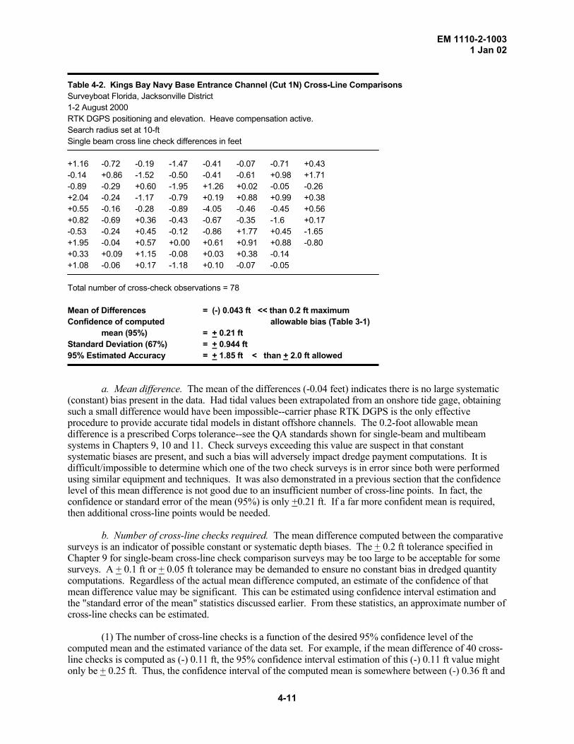
Table 4-2. Kings Bay Navy Base Entrance Channel (Cut 1N) Cross-Line Comparisons Surveyboat Florida, Jacksonville District 1-2 August 2000 RTK DGPS positioning and elevation. Heave compensation active. Search radius set at 10-ft Single beam cross line check differences in feet +1.16 -0.72 -0.19 -1.47 -0.41 -0.07 -0.71 +0.43 -0.14 +0.86 -1.52 -0.50 -0.41 -0.61 +0.98 +1.71 -0.89 -0.29 +0.60 -1.95 +1.26 +0.02 -0.05 -0.26 +2.04 -0.24 -1.17 -0.79 +0.19 +0.88 +0.99 +0.38 +0.55 -0.16 -0.28 -0.89 -4.05 -0.46 -0.45 +0.56 +0.82 -0.69 +0.36 -0.43 -0.67 -0.35 -1.6 +0.17 -0.53 -0.24 +0.45 -0.12 -0.86 +1.77 +0.45 -1.65 +1.95 -0.04 +0.57 +0.00 +0.61 +0.91 +0.88 -0.80 +0.33 +0.09 +1.15 -0.08 +0.03 +0.38 -0.14 +1.08 -0.06 +0.17 -1.18 +0.10 -0.07 -0.05 Total number of cross-check observations = 78 Mean of Differences = (-) 0.043 ft << than 0.2 ft maximum Confidence of computed allowable bias (Table 3-1) mean (95%) = + 0.21 ft Standard Deviation (67%) = + 0.944 ft 95% Estimated Accuracy = + 1.85 ft < than + 2.0 ft allowed a. Mean difference. The mean of the differences (-0.04 feet) indicates there is no large systematic (constant) bias present in the data. Had tidal values been extrapolated from an onshore tide gage, obtaining such a small difference would have been impossible--carrier phase RTK DGPS is the only effective procedure to provide accurate tidal models in distant offshore channels. The 0.2-foot allowable mean difference is a prescribed Corps tolerance--see the QA standards shown for single-beam and multibeam systems in Chapters 9, 10 and 11. Check surveys exceeding this value are suspect in that constant systematic biases are present, and such a bias will adversely impact dredge payment computations. It is difficult/impossible to determine which one of the two check surveys is in error since both were performed using similar equipment and techniques. It was also demonstrated in a previous section that the confidence level of this mean difference is not good due to an insufficient number of cross-line points. In fact, the confidence or standard error of the mean (95%) is only +0.21 ft. If a far more confident mean is required, then additional cross-line points would be needed. b. Number of cross-line checks required. The mean difference computed between the comparative surveys is an indicator of possible constant or systematic depth biases. The + 0.2 ft tolerance specified in Chapter 9 for single-beam cross-line check comparison surveys may be too large to be acceptable for some surveys. A + 0.1 ft or + 0.05 ft tolerance may be demanded to ensure no constant bias in dredged quantity computations. Regardless of the actual mean difference computed, an estimate of the confidence of that mean difference value may be significant. This can be estimated using confidence interval estimation and the "standard error of the mean" statistics discussed earlier. From these statistics, an approximate number of cross-line checks can be estimated. (1) The number of cross-line checks is a function of the desired 95% confidence level of the computed mean and the estimated variance of the data set. For example, if the mean difference of 40 cross-line checks is computed as (-) 0.11 ft, the 95% confidence interval estimation of this (-) 0.11 ft value might only be + 0.25 ft. Thus, the confidence interval of the computed mean is somewhere between (-) 0.36 ft and

4-11

EM 1110-2-1003 1 Jan 02 (+) 0.14 ft. This may or may not be an acceptable range, nor is there much confidence in the accuracy of the (-) 0.11 mean difference. What this indicates is that in insufficient number of cross-lines were obtained. The + 0.25 ft "standard error of the mean" is large--more data comparisons are required to reduce this range down to an "acceptable" level. The estimated variance of the data also affects the confidence of the computed mean. Fewer checks would be required for tightly grouped data--e.g., < 15-ft shallow draft work with an estimated 95% accuracy of + 0.25 ft (Table 3-1). (2) The following is a tabulation of the theoretical number of cross-lines required for a given survey accuracy (Table 3-1). Numbers of comparisons are computed for different confidence levels of the computed mean. These are computed by solving for n in the standard formula:

Standard error of the mean (95%) = + 1.96 ( σ / n ½ ) (Eq 4-5)

where σ = population standard error (i.e., estimated 1-σ accuracy at various project depths) n = number of observations Table 4-3. Cross-line Comparisons Required for Different Confidence Intervals Estimated Depth Accuracy Confidence Interval of Computed Mean (95%) 95% * + 0.2 ft +0.1 ft + 0.05 ft + 0.25 ft 2 6 24 + 0.5 ft 6 24 96 + 1.0 ft 24 96 384 + 2.0 ft 96 384 1536 * These 95% values relate to estimated depth accuracies in Table 3-1. The 1-σ deviation is used in the computation From the above tabulation, it is clear that the computed mean for lead line surveys in shallow water can be determined with relatively few cross-line checks. This is because the expected depth accuracy is good in shallow depths. The number of cross-line checks increases as the desired confidence level in the mean difference increases. For less accurate acoustic surveys in deeper water depths, more comparison points are required. In a deep-draft 50-ft project, at least 100 check points should be obtained to ensure a + 0.2 ft confidence in the mean. Higher confidence levels would require an impractical number of comparisons for most single-beam cross-section surveys--only overlapping multibeam or multiple transducer surveys could (economically) obtain these higher numbers. (3) Although cross-check line checks are required as a QA process in single-beam survey (Chapter 9), the resultant value of the mean difference must account for the statistical uncertainty in the computation--plus the fact that the surveys may not be independent. With few cross-line check points, the apparent mean difference between the surveys is, at best, only a rough indicator of the true difference. It is, however, better than having no QA comparison, and will indicate any large blunders that may exist. c. Standard deviation. The standard deviation computed at the one-sigma level is adjusted to the 95% confidence level. This 95% deviation (+ 1.85 ft) in Table 4-2 is typical of results in deep-draft navigation channels of uneven topography. It is, however, less than the + 2.0 ft allowable accuracy defined in Table 3-1 for project depths greater than 40 feet. Without RTK vertical elevations and heave compensation, the deviation would have been much larger--probably exceeding the allowable tolerance.

4-12

EM 1110-2-1003 1 Jan 02

Some of the variation could be attributable to the uneven bottom topography coupled with the 10-ft HYPACK search radius. The footprint size of the acoustic beam covers a larger area in these 50-foot depths, causing a generalization in the recorded depths. In general, however, standard deviations at this level would be expected based on the estimated results back in Table 4-1 and the fact that this distant project area represents a "worst case" condition than that assumed in Table 4-1. (Note that the computed standard deviation is not the same as the RMS in that the (-) 0.04 ft is not included. The difference is negligible given the small mean bias--the RMS (95%) could be computed from Equation 4-1, e.g., RMS (95%) = 1.96 (0.944 2 + 0.043 2 ) 1/2 = + 1.85 ft). Like the computed mean above, the confidence level of the computed deviation could also have been computed--Mikhail, 1976. Such a computation would have shown that the + 0.94 standard deviation actually lies somewhere between + 0.8 and + 1.2 (95% confidence level). Additional cross-line comparisons would have reduced this spread. d. Multiple transducer or multibeam comparison. Had the above project been surveyed using swath survey systems, then two digital elevation models could have been generated with which to perform a comparison. Thousands of comparison points would have resulted rather than the 78 in the single beam example. Regardless of the number of comparative points, the computed mean and deviation should not be significantly different--at least within the range of the confidence interval estimations described above. The standard deviation of multibeam data might be slightly higher since the accuracy of the outer rays is not as good as near-vertical depths. However, the confidence level of the mean would have a very small value since a larger number of points are included. e. Unaccounted biases. It is again emphasized that such comparisons are only indicators of data quality. There could be biases in the data that would not be detected. Examples might include: (1) a constant error in the tidal datum reference plane or MLLW elevation reference, (2) an error in the DGPS vertical geoid model, or (3) a constant vessel draft error. Data outliers can also be present in the data, such as the 4.05 foot difference in Table 4-2. These outliers represent values well outside the 95% confidence level. They may or may not be correct. Typically, outliers falling more than 3 times the estimated standard error (i.e., 3 · 0.944 ft) are rejected. f. Final analysis of results. The nearly + 2 foot depth deviation in this example clearly exhibits the case that individual depth observations contain significant random errors. It also illustrates that a single depth observation cannot be evaluated based on the "apparent accuracy" of its plotted value (i.e., nearest 0.1 foot). Moreover, this case shows that the accuracy of a survey must be evaluated based on the statistical agreement of the entire data set--or portions of that data set. Minimizing constant bias errors is far more important than reducing deviations. More refined acoustic measurement techniques will have to be developed if more accurate depth observations are required. 4-8. Evaluation of Depth Accuracy on Dredging Projects Evaluating channel clearance on dredging projects involves a review of the soundings obtained on the final after dredge survey and/or final channel clearance sweep survey. Numerous shoals or strikes above the required grade may be present on these surveys. The project manager or contracting officer's representative (COR) must determine whether these shoals/strikes above grade warrant additional work effort to assure project clearance, or they are isolated, stray soundings within the "noise" (i.e., accuracy) level of depth measurement. Therefore, this assessment of above-grade soundings must consider (1) the error budget of individual depth measurements, (2) their relative magnitude, (3) survey accuracy standards specified for the project--Table 3-1, and (4) the detection repeatability of the acoustic system. a. The object detection standard in Table 3-1 specifies that a minimum of three acoustic "hits" be obtained on a potential shoal or strike. These hits should ideally be obtained on repeated passes over an object. A single pass is adequate if numerous hits above grade are obtained, and the depths are consistently above the required grade.

4-13

EM 1110-2-1003 1 Jan 02 b. A single hit 0.1-ft to 0.5-ft above grade presents problems. This hit could be the edge of a shoal or rock of larger size and shoaler elevation. If the estimated accuracy of the depth measurement process used is + 1.0 ft, then this could be an observation lying within that 95% accuracy tolerance--e.g., taken when a vessel without heave compensation was surging down in the trough of a wave. Such a potential variation between depths and surveys is clearly exhibited in Table 4-2. Thus, additional observations are needed to confirm the existence (or non-existence) of material lying above the project grade. Additional passes should be run over the area. If acoustic hits above grade are repeatedly obtained on these additional passes, then a high probability exists that a shoal or rock strike is present in the channel. The confidence levels of shoal detection can be estimated given (1) height of hits above grade (dZ), (2) standard error of depth measurements (s), and (3) number of hits (n). Using approximate t-density functions, it can be shown that all three of the above factors (variables) will determine the overall confidence of detection, which can be roughly computed by the following: t α/2, n-1 ≈ sqrt ( n ) ( dZ ) / s For example, given 3 hits averaging 1-ft above grade and a + 1.0 ft standard error, the detection confidence is roughly 75%. If only 2 hits were recorded, the confidence of a shoal drops to 60%. If 10 hits are recorded, the confidence of detection is 98%. Thus, obtaining a 95% detection confidence may require more than 3 hits, depending on the magnitude of the three variables described above. c. Obtaining multiple hits with a single, narrow beam echo sounder is difficult. Stealth-like objects may not always be detected with vertical beams. Close line spacing must be run over a suspected strike--e.g., 10 ft to 20 ft intervals. A multiple transducer or multibeam system is far more efficient in detecting strikes and confirming them with multiple passes. Multibeam sweeps should be conducted such that the beam aspect is varied from near-vertical to an outside beam. Multibeam side scan imagery on the outer beams will also be of value in detecting strikes above grade. On critical projects, towed side scan may be necessary to locate strikes. d. The relative height of an object or shoal above grade will determine the need for clearance. This may depend on the location of the shoal within the channel, type of bottom material, size of shoal, potential navigation hazard, etc. The project COR makes the final determination on whether to mobilize or remobilize a dredge to remove the object/shoal. 4-9. Evaluation of Dredge Quantity Estimates Based on Depth Accuracy and Density Three primary factors impact the accuracy of dredge volume computations, in this order:

• Terrain irregularity and data density

• Bias errors in depth measurements

• Deviation of depth observations It has been shown that data density has the most important effect on the overall accuracy of a quantity computation. Required data density is a function of the irregularities in the terrain, as is clearly illustrated in Figure 4-3. Systematic biases in the depth database will obviously cause constant dredge volume errors. The deviation or estimated accuracy of the depths can cause volume errors if the standard error is large and an insufficient number of points are observed. A volume derived from a densely gridded/binned multibeam survey will yield a more accurate quantity than that obtained from 100-ft spaced cross-sections, even if the depth accuracy (i.e., standard deviation) of the multibeam survey is not a good as the cross-section depths. These concepts are discussed below.

4-14

EM 1110-2-1003 1 Jan 02

Figure 4-3. Single beam versus multibeam coverage--Port of Los Angeles. Drawings compare low density single beam coverage (bottom view) with detailed multibeam coverage (top view). Dredged sections are

generalized in the single beam coverage. (Coastal Oceanographics, Inc. and Los Angeles District) a. Terrain irregularity impacts on volume accuracy. The effects of terrain irregularities on dredge volume computations depend on the density of data coverage. When end areas are computed for single-beam cross-sections, large variations in the end areas would indicate terrain irregularity exists between the sections. Even if the cross-section data points were absolutely error-free (no bias or standard deviation) large volume errors due to terrain irregularity would still exist due to lack of measurements between the 100-ft sections. These effects can be illustrated by the following single-beam survey example. Given: Typical 400-ft wide box-cut channel (no side slope quantities computed) Predredge shoaling fairly uniform at around 10 feet above pay grade 100-ft cross-sections run over 3,000 ft Acceptance Section Standard average-end-area volume computation Station Cross-sectional End Area 60+00 3850 sq ft 61+00 4125 62+00 3975 63+00 4225 64+00 4150 . . . 89+00 4125 90+00 3950 (1) In looking at the variations in end areas for the 31 cross-sections, it is determined that their average deviation is approximately + 100 sq ft. If depth measurement biases and deviations are assumed to be zero, then this end-area variance between cross-sections in a uniform shoal area is due to irregularities in

4-15

EM 1110-2-1003 1 Jan 02 the terrain. Had cross-sections been observed at 1-ft intervals (e.g., multibeam) then the end-area variations would be expected to be significantly less. The volume error over due to this +100 sq ft can be computed by comparing the quantities over the section for a 4,000 sq ft and 4,100 sq ft end area. The percentage quantity error is simply: % error in volume = (100 sq ft / 4000 sq ft ) · 100% = 2.5 % This 2.5 % error equates to 370 cy per 100-ft section or about 11,000 cy over the entire acceptance section (which has a total yardage of nearly 450,000 cy). (2) Had the bottom terrain been more uniform, then the computed end-area variations would be smaller. A variation of + 20 sq ft would have represented only a 0.5 % error on this project. If the end-areas were linearly increasing or decreasing (sloping shoal), then this slope would be considered in looking at variations in end areas. On the other hand, had there only been an average of 4 feet of shoaling above grade, then the relative volume error would be larger--i.e., (100 sq ft/1,600 sq ft) · 100% = 6.25%. (3) Minimizing end-area volume errors due to terrain irregularities between single-beam cross sections is often impractical. Since the only way to minimize the error is to decrease line spacing, practical limitations prevent this. Decreasing line spacing to, say 20 ft, adds field survey time and cost. In addition, a 20-ft line spacing is near the tolerance of the ability to control the survey vessel on line. Since most average-end-area computations assume cross-sections are equally spaced--i.e., no off line steering deviations--projecting these lines over 20-ft distances is no longer valid. However, given the sparse cross-sections data sets, a TIN model may be generated for all the observed data points and volumes computed using the vertical TIN prismoidal elements rather than average-end-area projections. This would represent a more accurate volume computation than average-end-area methods. See additional discussion in Chapter 15 (Dredge Measurement and Payment Volume Computations). b. Impact of depth measurement bias errors on volume computations. The causes of depth bias in a data set were discussed in the preceding paragraphs. A constant depth bias in the data set is estimated from cross-line checks or multibeam performance test data. The effect of a constant depth bias on a dredged quantity computation is fairly obvious--the error projects over the entire dredging section (e.g., Acceptance Section). Thus, minimizing any depth biases is critical. Using the 3,000 ft acceptance section in the above example, the quantity error due to a 0.1 ft depth bias can be approximately computed by projecting the bias over the entire section: volume error = 0.1 ft · 400 ft · 3,000 ft / (27 cy/ft) = 4,450 cy percent error = 4,450 cy / 450,000 cy = 1 % In the above example, it is seen that the bias error (1%) is smaller than the error due to terrain variations (2.5%). This corresponds to theory and is roughly what occurs in practice. Bias error can become more significant in offshore tidal areas where modeling becomes difficult. c. Impact of deviations in depth observations on volume computations. From the sample computation from the Kings bay project cross-line data in Table 4-2, the standard deviation of the depth measurements was estimated to be + 0.9 ft, or + 1.8 ft at the 95% level. If there are no biases in the data, volumes computed over a given area from an infinite number of observed data points would have no error due to inaccuracies in individual depths. However, an infinite number of points are never observed. When single-beam cross-sections are taken, "full-coverage" is observed along the section if depths are recorded at intervals of 10-15 per sec. Normally, however, for both single-beam and multibeam surveys, data sets are generalized or "thinned"--i.e., binned or gridded. For example, single-beam cross-section data collected at 1-ft intervals may be generalized to points every 5- or 25-ft along the line, or dense multibeam data may be generalized into one data point in a 5 x 5 ft (25 sq ft) cell. This generalization is usually performed to reduce the size of the database. Either an average of all the points in a range or area is used or a single point

4-16

EM 1110-2-1003 1 Jan 02

nearest the cell center is used. The following over-simplified example illustrates how the data point accuracy and number of points can affect the dredge quantity computation. Given: 100-ft single beam cross-section run over 26.0 ft lock chamber

OFFSET DEPTH Depth Used 0 26.1 26.1 5 26

10 26 15 26 20 26.2 25 26 26 30 25.9 35 25.9 40 26 45 26.2 50 25.9 25.9 55 26 60 26 65 25.8 70 25.9 75 26.3 26.3 80 26 85 25.7 90 26.1 95 26

100 26.2 26.2

(1) The mean of the 21 depths observed at 5-ft intervals is 26.0 ft and their 1-σ standard deviation is + 0.14 ft. This indicates no bias in the data was observed in this dataset. The 95% confidence of the mean is + 0.06 ft. Thus, if all the points were used to compute an end-area of this cross-section, the accuracy of the end area would be good.

(2) If depths were thinned to the even 25-ft intervals as shown in the above table, and only these

depths used to compute the end-area of the cross-section, the end area accuracy would degrade significantly due to the few data points used. In this example, the mean of the five points is 26.1 ft, which, in effect adds a false 0.1 ft bias to the data. This 0.1 ft bias would be projected over the project area. The 95% confidence of this mean is also only (roughly) + 0.14 ft., indicating little confidence in the measurements and ultimately the volume.

(3) The above illustrates that higher data density improves volume accuracy, either for average-end-

area cross-sections or full DEM/DTM binned models. Larger numbers of data points negates out random errors in the individual data points. Improperly thinning datasets will cause errors in the volumes. The values from Table 4-3 may be used to roughly estimate the number of points needed along a cross-section to ensure some level of confidence in the end-area. For example, to maintain a confidence level of + 0.05 ft on a 30-ft project (estimated 95% depth accuracy is + 1.0 ft), at least 400 points should be collected. For a shallow-draft project, then only 100 data points would be needed to ensure + 0.05 ft confidence.

d. Conclusions. (1) Terrain irregularity has the major impact on the accuracy of volume computations. These

effects are minimized by increasing data density and using spatial volume computation methods. Average-

4-17

EM 1110-2-1003 1 Jan 02 end-area volume computation methods should only be used on projects with relatively uniform bottom terrain and where linearized end-area variations between successive sections are less than 0.5%. If end-area variations are large due to irregular bottom topography, then closer spaced cross-sections should be run or full-coverage multibeam surveys obtained.

(2) When sparse data sets (i.e., cross-sections) are observed, TIN or dense grid volume computation

methods using prismoidal projection elements are more accurate than average-end-area methods. If full multibeam datasets are observed, volumes should not be computed by passing sparse cross-sections through the dataset and using average-end-area methods.

(3) Collected survey data used for volume computations should not be thinned in order to minimize

volume errors due to data density and data point variance. If thinning is needed due to data processing limitations, it should be kept to a minimum. The degree of bottom irregularity will determine the amount of allowable thinning--i.e., maximum cell size. All observed depths on single beam surveys should be used in computing end-areas. For multibeam surveys, cell sizes should generally not exceed 5x5 ft bins. The smallest bin size that can be efficiently computed should always be used.

(4) Other factors may impact dredge volumes. These may include errors due to fluff, vegetation,

short-term draft or velocity variations, or sensitivity drift. These errors are difficult or impossible to quantify.

4-10. Horizontal Positioning Accuracy Estimates The horizontal position accuracy standard specified in Table 3-1 is a two-dimensional circular (radial) accuracy measure. A circular accuracy is an approximate estimate in that it approximates a 2-D error ellipse, as shown in Figure 4-4. The Federal (FGDC) and Corps positional accuracy standard is specified relative to this 95% confidence level. This means that on average 19 of 20 observed positions will fall within the required standard. The standard could be evaluated by comparing the observed position with a higher accuracy position. In a static mode, this can be done by recording DGPS positions with the receiving antenna set up over a known geodetic control point. Differences in X and Y coordinates between the known position and observed position are recorded, RMS errors are computed for each coordinate, and the two-dimensional positional error is estimated at the 95% level. It is far more difficult to evaluate the positional accuracy on a moving vessel since a more accurate position is not easily obtained with which to compare the observed position.

4-18

EM 1110-2-1003 1 Jan 02

1-Sigma (39%) error ellipse with axis dimensions “a” and “b”s X and s Y are distances to tangents

95 % Errorr 95% = 1.73 * r 63% Circular standard error (39%)

SC ≈ 0.5 (sX+sY) “CSE”

63% (1DRMS) ≈ 1.414 SC

95% ≈ 2.447 SC

98% (2DRMS) ≈ 2.828 SC

sx

sy

95% confidence is standardstatistical measure used for assessing a map feature accuracy

a b

1DRMS (63 %)r 63% = (s x

2 + s y 2 )1/2

CSE (39 %)s c = 0.5 (s x + s y )

2DRMS (98 %)

Figure 4-4. Two-dimensional radial positional accuracy estimates a. Two-dimensional elliptical positional accuracy. Computed horizontal positions from surveying measurements produce coordinate pairs on a flat map of two dimensions. The ellipse in Figure 4-4 represents a joint probability distribution of the errors in the X and Y directions. This elliptical distribution assumes no biases are present in the data. It represents a 39% probability. The dimensions of the ellipse are defined by its two axes—a and b—and its orientation relative to the X-Y grid. The standard error in each X-Y dimension is defined by the lengths of the tangents to the ellipse--sx and sy --as shown in Figure 4-4. This ellipse will have standard deviations sx, sy, and correlation (sxy) unless the axes of the ellipse are oriented parallel with the coordinate system axes. These standard deviations are computed directly from the ellipse’s dimensions and orientation. The probability of locating a randomly selected computed position within a standard error ellipse is 39.4%. Any error in the x or y direction will distort the ellipse in a perpendicular sense to show the magnitude of the error. The two-dimensional ellipse in Figure 4-4 indicates the x coordinate component has the greatest error. Often, however, constant positional biases may be present. These biases may exceed the apparent dispersion levels of the data. The biases must be included in any estimate of the 95% positional confidence. b. Two dimensional error measures. The error ellipse refers to probability as a measure of survey precision quality. If the circle (special case of an ellipse) could represent the error, then one number could define the precision of survey measurements. A radial error measure is used to approximate the ellipse. The radius r of the Circular Standard Error (CSE) circle is computed from the standard deviations--sx and sy –in the error ellipse, as shown in the figure. This CSE circle represents a 39% probability. A more common circular approximation is the 63% circle, or 1DRMS. It is computed by taking the square root of the sum of the variances in x and y. It may also be approximated by multiplying 1.1414 times the average of the standard deviations—a valid assumption if the ellipse is nearly circular. The 63% 1DRMS circle is also known as a 1-deviation RMS--i.e., 1DRMS. A 2DRMS is defined as two deviations of circular error with probabilities of approximately 98%. The 95% error circle shown in Figure 4-4 is 1.73 times the radius of the 1DRMS circle. GPS manufacturers typically use a 2DRMS (i.e., approximately 98%) measure of positional accuracy, not the 95% radial accuracy measure used by FGDC and this manual. Another circular error approximation is the Circular Probable Error (CPE)—a 50% probability. Errors computed by the

4-19

EM 1110-2-1003 1 Jan 02 statistical methods are linked to the probabilities that the actual error at a given point will not exceed the computed error value. The actual error at the given point may be far less. Probabilities predict computed errors based on the theory of repeated trials. In mapping, repeated measurements are rare and the actual error is unknown except for upper and lower limits. See Bowditch, 1984 for additional information. c. Horizontal positioning error components. The estimated accuracy A of a vessel's offshore position can be generalized by the following expression (in matrix form):

Two-dimensional Accuracy A = σ0 2 · Q (Eq 4-6)

where σ0 is the estimated standard error of each component of the particular positioning system used (tag line, microwave range, GPS satellite range, etc.). Each measurement component may have different estimated standard errors. Variable Q (cofactor matrix) is a two-dimensional geometric factor associated with intersection angles of ranges or angles used to coordinate the offshore point (circular range-range intersection, circular range-transit azimuth intersection, or multiple range intersections). (1) The resultant estimated accuracy A is a two-dimensional term containing the variances and covariances of the particular observation. A reduced form is usually best represented by an ellipse (see Figure 4-4) since the geometrical component Q influences the accuracy in varying magnitude and direction. (2) Standard error of individual observations. The standard error (σ0) term is a function of the estimated accuracy of the measurement system, including survey methods and techniques used to calibrate the system. Each EDM or GPS satellite range will have a standard error associated with it. This standard error is not the internal precision of the range measurement. It must additionally include an estimate of the systematic (or constant) biases present. As explained earlier, determining the standard error (or standard deviation) of a dynamic hydrographic distance measurement is extremely difficult and can only be roughly estimated from a limited number of static calibration checks. For example, estimates of a total station EDM range measurement will normally be based on the unbiased standard deviation of the calibration comparisons over a fixed baseline, namely: σ = sqrt [ Σ (X i - X m ) 2 ] / [n – 1]

(Eq 4-7) where X i = Observed distance observation n = number of observations (i = 1 through n)

X m = mean of all observations (3) Average deviation. For many practical survey purposes, it is often simpler to compute the “average deviation” rather than the standard deviation: Average deviation = [ Σ |X m - X i | ] / n

(Eq 4-8) where Σ|Xm - Xi| is the sum of the absolute values of the deviations (signs disregarded).

(4) Geometrical factors. This can be the major error component in the resultant accuracy of an offshore position. All offshore positioning methods commonly used on engineering surveys reduce to determining the coordinate intersection of two or more lines that have been generated by constant distances

4-20

EM 1110-2-1003 1 Jan 02

or angles from the reference points ashore or from satellites. These lines are often termed “lines of position.” The relative strength of a position is a direct function of the angle of intersection between these lines. The strongest position “fix” is usually obtained when two position lines intersect at 90 deg. As the angle of intersection deviates from 90 deg, the relative strength of position weakens. In positioning systems in which the standard error increases with distance offshore (e.g., total station range azimuth), the strength of position will also vary with the distance from the observing unit. Systems that observe more than two lines of position are termed “redundant” or “multi-ranging.” GPS satellite position involves four or more lines of position. The angle by which these three or more lines intersect is also factored into this geometrical component, although in a more complex manner. When the standard error components are plotted (at a large scale) for each line of position, the intersections can be generalized to a trapezoidal figure (in the case of two observations only) which roughly depicts the 2-D positional error. From this plot and/or data, a standard error ellipse of constant probability can be derived. The size and shape of this error ellipse vary directly with the angle of intersection between the lines of position and the range error. The one-sigma standard error ellipse is a figure that represents a 0.39 probability; or there is a 39-percent chance that the position falls somewhere within this ellipse. Conversely, there is a 61-percent probability that the position falls outside the ellipse—see Figure 4-3. Due to changing geometry, the size and direction of the error ellipse will vary as a survey vessel traverses from point to point in a project area. Particular note should be made that the uncertainty of a position can be several magnitudes larger along one (semi-major) axis. This may be significant on some projects where detail is critical in one dimension. The error ellipse is only a graphical representation (or approximation) of a position's estimated accuracy. For a number of reasons, because of the non-random (or non-normal) distribution of errors in surveys, this representation must be considered approximate. Since error ellipses are difficult to conceptualize, an elliptical positional accuracy estimate is usually approximated by a circle whose radius represents some function of the ellipse's axes--e.g., CSE, 2DRMS. d. Geometrical Dilution of Precision (GDOP). Another statistic commonly used in static and kinematic GPS surveying is the Geometric Dilution of Precision (GDOP). This term is directly related to the Q term in Equation 4-6, and is used as an indicator of a position's degradation due to changing intersection geometry. For the simple case of a 2-D horizontal position, the term Horizontal Dilution of Precision (HDOP) is used. HDOP is computed as follows:

HDOP = Tr |Q | / σ 0 = [ σX2 + σY

2 ] / σ 0 (Eq 4-9)

where Tr |Q | is the trace of the Q matrix and σ 0 is the assumed accuracy of a satellite or EDM range measurement. For a positioning system of given accuracy and a desired horizontal accuracy limit, a maximum HDOP limit may be established. Data points outside this HDOP would be rejected. Since HDOP varies with location on non-GPS surveys, it is applicable only to a static point. In the case of a hydrographic survey being positioned using differential GPS, the moving reference satellites will vary the GDOP/HDOP with time rather than position in a given project area. This is opposite to the case of a vessel moving relative to the fixed EDM (or angular) reference stations.

4-21

EM 1110-2-1003 1 Jan 02 4-11. FGDC Accuracy Reporting Criteria The FGDC Geospatial Positioning Accuracy Standards, Part 3: National Standard for Spatial Data Accuracy uses root-mean-square error (RMSE) to estimate positional accuracy. The FGDC defines RMSE as the square root of the average of the set of squared differences between dataset coordinate values, and coordinate values from an independent source of higher accuracy for identical points. RMS errors are computed for both the X and Y coordinates, then are combined to obtain a 95% positional accuracy estimate--see FGDC reference at end of chapter. Accuracy is reported in ground distances at the 95% confidence level. Accuracy reported at the 95% confidence level means that 95% of the positions in the dataset will have an error with respect to true ground position that is equal to or smaller than the reported accuracy value. The reported accuracy value reflects all uncertainties, including those introduced by geodetic control coordinates, compilation, and final computation of ground coordinate values in the product.

a. Horizontal. The reporting standard in the horizontal component is the radius of a circle of uncertainty, such that the true or theoretical location of the point falls within that circle 95% of the time.

b. Vertical. The reporting standard in the vertical component is a linear uncertainty value, such that the true or theoretical location of the point falls within + of that linear uncertainty value 95-percent of the time. The reporting accuracy standard should be defined in metric (International System of Units, SI) units. However, accuracy will be reported in English (inch-pound) units where the point coordinates or elevations are reported in English units. Corps position and elevation (depth) accuracy statistics, accuracy assessment techniques, and reporting methods, as defined in this manual, are designed to conform to the above FGDC standards. 4-12. References Bowditch 1984 Bowditch, Nathaniel, The American Practical Navigator: An Epitome of Navigation, Appendix Q: Navigational Accuracy, Defense Mapping Agency Hydrographic/Topographic Center, 1984 Mikhail 1976 Mikhail, Edward M., Observations and Least Squares, 1976 4-13. Mandatory Requirements There are no mandatory requirements in this chapter.

4-22