Chapter 4: sem in R and in LISREL - Personality Project · code for many problems in LISREL and EQS syntax, Raykov and Marcoulides (2006) give examples in EQS, LISREL and Mplus. In

Chapter 4: sem in R and in LISREL

William RevelleNorthwestern University

Prepared as part of course on latent variable analysis (Psychology 454)and as a supplement to the Short Guide to R for psychologists

February 14, 2007

4.1 Example data set 1: 9 cognitive variables (from Rakov and Marcoulides) . . . . 14.2 Using R to analyze the data set . . . . . . . . . . . . . . . . . . . . . . . . . . . 3

4.2.1 An initial formulation is empirically underidentified . . . . . . . . . . . 34.2.2 Adjusting to model to converge . . . . . . . . . . . . . . . . . . . . . . . 44.2.3 Modifying the model to improve the fit . . . . . . . . . . . . . . . . . . 74.2.4 Changing from a regression model to a correlation model . . . . . . . . 9

4.3 Using LISREL to analyze the data set . . . . . . . . . . . . . . . . . . . . . . . 114.3.1 Instructions for using the SSCC . . . . . . . . . . . . . . . . . . . . . . . 114.3.2 Modify the model to allow for correlated errors . . . . . . . . . . . . . . 20

4.4 Comparing the R and LISREL output . . . . . . . . . . . . . . . . . . . . . . . 284.5 Testing for factorial invariance . . . . . . . . . . . . . . . . . . . . . . . . . . . 28

4.5.1 Testing for factorial equivalence in multiple groups . . . . . . . . . . . . 304.6 References . . . . . . . . . . . . . . . . . . . . . . . . . . . . . . . . . . . . . . . 31

There are many programs that allow one to analyze latent variable models. Almost allstatistical packages will include the ability to do exploratory factor analysis and many allow forconfirmatory analysis. Commerically available sem programs include AMOS, EQS, LISREL,MPlus, and SAS. Open source programs include R and Mx. The Loehlin text gives samplecode for many problems in LISREL and EQS syntax, Raykov and Marcoulides (2006) giveexamples in EQS, LISREL and Mplus. In this chapter we compare the set up and output ofthe sem package in R with the unix version of LISREL for several problems.

4.1 Example data set 1: 9 cognitive variables (from Rakovand Marcoulides)

Tenko Raykov and George Marcoulides, in their textbook on SEM (Rakov and Marcoulides,2006), present a data set based upon 220 high school students on 9 cognitive measures.They report three measures of Induction taken in the junior year, three measures of FiguralRelations in the junior year, and three measures of figural relations in the senior year.

1

http://personality-project.org/revelle.html

http://personality-project.org/revelle/syllabi/454/454.syllabus.pdf

http://personality-project.org/

Induction Figural Fig2

Induction1 Induction2 Induction3 Figural1 Figural2 Figural3 Fig2_1 Fig2_2 Fig2_3

Figure 4.1: 9 cognitive variables (adapted from Raykov and Marcoulides, 2006)

They present the data set as a lower triangular covariance matrix which we can read thisinto R using the scan function embedded in a function to convert the data to a rectangularmatrix:

> lower.triangle <- function(nrow = 2, data = NULL) {

+ if (is.null(data))

+ data <- scan(pipe("pbpaste"))

+ mat <- diag(0, nrow)

+ k <- 1

+ for (i in 1:nrow) {

+ for (j in 1:i) {

+ mat[i, j] <- data[k]

+ k <- k + 1

+ }

+ }

+ mat <- mat + t(mat)

+ diag(mat) <- diag(mat)/2

+ return(mat)

+ }

p5.in <- scan("")56.2131.55 75.5523.27 28.30 44.4524.48 32.24 22.56 84.6422.51 29.54 20.61 57.61 78.9322.65 27.56 15.33 53.57 49.27 73.7633.24 46.49 31.44 67.81 54.76 54.58 141.7732.56 40.37 25.58 55.82 52.33 47.74 98.62 117.3330.32 40.44 27.69 54.78 53.44 59.52 96.95 84.87 106.35

prob5 <- lower.triangle(9,p5.in)

> colnames(prob5) <- rownames(prob5) <- c("Induct1", "Induct2", "Induct3", "Figural1", "Figural2",

+ "Figural3", "Fig2.1", "Fig2.2", "Fig2.3")

> prob5

Induct1 Induct2 Induct3 Figural1 Figural2 Figural3 Fig2.1 Fig2.2 Fig2.3Induct1 56.21 31.55 23.27 24.48 22.51 22.65 33.24 32.56 30.32Induct2 31.55 75.55 28.30 32.24 29.54 27.56 46.49 40.37 40.44

2

Induct3 23.27 28.30 44.45 22.56 20.61 15.33 31.44 25.58 27.69Figural1 24.48 32.24 22.56 84.64 57.61 53.57 67.81 55.82 54.78Figural2 22.51 29.54 20.61 57.61 78.93 49.27 54.76 52.33 53.44Figural3 22.65 27.56 15.33 53.57 49.27 73.76 54.58 47.74 59.52Fig2.1 33.24 46.49 31.44 67.81 54.76 54.58 141.77 98.62 96.95Fig2.2 32.56 40.37 25.58 55.82 52.33 47.74 98.62 117.33 84.87Fig2.3 30.32 40.44 27.69 54.78 53.44 59.52 96.95 84.87 106.35

4.2 Using R to analyze the data set

The model proposed for this is that Induction in year1 predicts Figural Ability in Year 1 andYear 2 and that Figural Ability in Year 1 predicts Figural Ability in Year 2.

4.2.1 An initial formulation is empirically underidentified

The R code for doing the basic analysis is straightforward:

path label initial estimate[1,] "Induction -> Induct1" NA "1"[2,] "Induction -> Induct2" "2" NA[3,] "Induction -> Induct3" "3" NA[4,] "Figural -> Figural1" NA "1"[5,] "Figural -> Figural2" "5" NA[6,] "Figural -> Figural3" "6" NA[7,] "Figural.time2 -> Fig2.1" NA "1"[8,] "Figural.time2 -> Fig2.2" "8" NA[9,] "Figural.time2 -> Fig2.3" "9" NA[10,] "Induction -> Figural" "i" NA[11,] "Induction -> Figural.time2" "j" NA[12,] "Figural -> Figural.time2" "k" NA[13,] "Induct1 <-> Induct1" "u" NA[14,] "Induct2 <-> Induct2" "v" NA[15,] "Induct3 <-> Induct3" "w" NA[16,] "Figural1 <-> Figural1" "x" NA[17,] "Figural2 <-> Figural2" "y" NA[18,] "Figural3 <-> Figural3" "z" NA[19,] "Fig2.1 <-> Fig2.1" "q" NA[20,] "Fig2.2 <-> Fig2.2" "r" NA[21,] "Fig2.3 <-> Fig2.3" "s" NA[22,] "Induction <-> Induction" "A" "1"[23,] "Figural <-> Figural" "B" "1"[24,] "Figural.time2 <-> Figural.time2" "C" "1"

Model Chisquare = 124 Df = 24 Pr(>Chisq) = 2.1e-15Chisquare (null model) = 1177 Df = 36Goodness-of-fit index = 0.88

3

Adjusted goodness-of-fit index = 0.78RMSEA index = 0.14 90% CI: (0.11, 0.16)Bentler-Bonnett NFI = 0.9Tucker-Lewis NNFI = 0.87Bentler CFI = 0.91BIC = -5.7

Normalized ResidualsMin. 1st Qu. Median Mean 3rd Qu. Max.

-1.55000 -0.47200 0.00098 0.14300 0.55700 3.20000

Parameter EstimatesEstimate Std Error z value Pr(>|z|)

2 1.3e+00 0.118 10.6 0.0e+00 Induct2 <--- Induction3 8.5e-01 0.100 8.5 0.0e+00 Induct3 <--- Induction5 9.3e-01 0.026 35.3 0.0e+00 Figural2 <--- Figural6 8.8e-01 0.021 42.0 0.0e+00 Figural3 <--- Figural8 8.8e-01 0.039 22.4 0.0e+00 Fig2.2 <--- Figural.time29 8.8e-01 0.028 31.8 0.0e+00 Fig2.3 <--- Figural.time2i 2.0e+00 NaN NaN NaN Figural <--- Inductionj -2.0e+03 NaN NaN NaN Figural.time2 <--- Inductionk 1.0e+03 NaN NaN NaN Figural.time2 <--- Figuralu 4.2e+01 4.210 10.0 0.0e+00 Induct1 <--> Induct1v 5.3e+01 5.350 9.9 0.0e+00 Induct2 <--> Induct2w 3.4e+01 3.391 10.0 0.0e+00 Induct3 <--> Induct3x 2.6e+01 3.040 8.5 0.0e+00 Figural1 <--> Figural1y 2.9e+01 3.535 8.2 2.2e-16 Figural2 <--> Figural2z 2.8e+01 3.382 8.3 0.0e+00 Figural3 <--> Figural3q 3.2e+01 4.232 7.5 8.5e-14 Fig2.1 <--> Fig2.1r 3.2e+01 4.058 8.0 1.8e-15 Fig2.2 <--> Fig2.2s 2.0e+01 3.050 6.6 3.6e-11 Fig2.3 <--> Fig2.3A 1.4e+01 NaN NaN NaN Induction <--> InductionB -7.0e-04 NaN NaN NaN Figural <--> FiguralC 7.4e+02 NaN NaN NaN Figural.time2 <--> Figural.time2

Iterations = 500

Aliased parameters: i j k A B C

4.2.2 Adjusting to model to converge

Unfortunately, the estimation in 4.2.1 does not converge and failed after 500 iterations. Thisis not an unusual problem in estimation. By specifying start values for the Induction ->Figural.time2 path, we can get a satsifactory solution:

4

path label initial estimate[1,] "Induction -> Induct1" NA "1"[2,] "Induction -> Induct2" "2" NA[3,] "Induction -> Induct3" "3" NA[4,] "Figural -> Figural1" NA "1"[5,] "Figural -> Figural2" "5" NA[6,] "Figural -> Figural3" "6" NA[7,] "Figural.time2 -> Fig2.1" NA "1"[8,] "Figural.time2 -> Fig2.2" "8" NA[9,] "Figural.time2 -> Fig2.3" "9" NA[10,] "Induction -> Figural" "i" NA[11,] "Induction -> Figural.time2" "j" NA[12,] "Figural -> Figural.time2" "k" "0.75"[13,] "Induct1 <-> Induct1" "u" NA[14,] "Induct2 <-> Induct2" "v" NA[15,] "Induct3 <-> Induct3" "w" NA[16,] "Figural1 <-> Figural1" "x" NA[17,] "Figural2 <-> Figural2" "y" NA[18,] "Figural3 <-> Figural3" "z" NA[19,] "Fig2.1 <-> Fig2.1" "q" NA[20,] "Fig2.2 <-> Fig2.2" "r" NA[21,] "Fig2.3 <-> Fig2.3" "s" NA[22,] "Induction <-> Induction" "A" "1"[23,] "Figural <-> Figural" "B" "1"[24,] "Figural.time2 <-> Figural.time2" "C" "1"

Model Chisquare = 52 Df = 24 Pr(>Chisq) = 0.00076Chisquare (null model) = 1177 Df = 36Goodness-of-fit index = 0.95Adjusted goodness-of-fit index = 0.91RMSEA index = 0.073 90% CI: (0.046, 0.1)Bentler-Bonnett NFI = 0.96Tucker-Lewis NNFI = 0.96Bentler CFI = 0.98BIC = -77


-9.5e-01 -8.9e-02 -7.3e-05 -1.2e-02 1.4e-01 1.3e+00


2 1.27 0.159 8.0 1.3e-15 Induct2 <--- Induction3 0.89 0.114 7.8 7.1e-15 Induct3 <--- Induction5 0.92 0.066 13.9 0.0e+00 Figural2 <--- Figural6 0.88 0.066 13.4 0.0e+00 Figural3 <--- Figural8 0.88 0.052 16.9 0.0e+00 Fig2.2 <--- Figural.time2

5

9 0.88 0.048 18.2 0.0e+00 Fig2.3 <--- Figural.time2i 0.98 0.147 6.6 3.6e-11 Figural <--- Inductionj 0.60 0.178 3.4 7.2e-04 Figural.time2 <--- Inductionk 0.81 0.110 7.4 1.5e-13 Figural.time2 <--- Figuralu 30.90 3.891 7.9 2.0e-15 Induct1 <--> Induct1v 34.83 5.067 6.9 6.2e-12 Induct2 <--> Induct2w 24.49 3.075 8.0 1.8e-15 Induct3 <--> Induct3x 22.83 3.450 6.6 3.7e-11 Figural1 <--> Figural1y 26.87 3.459 7.8 8.0e-15 Figural2 <--> Figural2z 26.33 3.353 7.9 4.0e-15 Figural3 <--> Figural3q 31.31 4.451 7.0 2.0e-12 Fig2.1 <--> Fig2.1r 32.17 4.043 8.0 1.8e-15 Fig2.2 <--> Fig2.2s 20.44 3.213 6.4 2.0e-10 Fig2.3 <--> Fig2.3A 25.31 5.156 4.9 9.1e-07 Induction <--> InductionB 37.70 6.085 6.2 5.8e-10 Figural <--> FiguralC 36.00 6.017 6.0 2.2e-09 Figural.time2 <--> Figural.time2

Iterations = 168

Std. Estimate1 0.67105 Induct1 <--- Induction2 2 0.73412 Induct2 <--- Induction3 3 0.67018 Induct3 <--- Induction4 0.85457 Figural1 <--- Figural5 5 0.81215 Figural2 <--- Figural6 6 0.80191 Figural3 <--- Figural7 0.88269 Fig2.1 <--- Figural.time28 8 0.85197 Fig2.2 <--- Figural.time29 9 0.89877 Fig2.3 <--- Figural.time210 i 0.62464 Figural <--- Induction11 j 0.28886 Figural.time2 <--- Induction12 k 0.60902 Figural.time2 <--- Figural

Induct1 Induct2 Induct3 Figural1 Figural2 Figural3 Fig2.1 Fig2.2 Fig2.3Induct1 0.00 -0.55 0.79 -0.23 -0.17 1.01 -2.15 1.49 -0.89Induct2 -0.55 0.00 -0.21 0.90 0.78 0.11 1.61 0.96 0.86Induct3 0.79 -0.21 0.00 0.62 0.47 -3.89 0.01 -2.02 -0.03Figural1 -0.23 0.90 0.62 0.00 0.88 -0.58 2.58 -1.46 -2.75Figural2 -0.17 0.78 0.47 0.88 0.00 -0.42 -5.11 -0.24 0.64Figural3 1.01 0.11 -3.89 -0.58 -0.42 0.00 -2.56 -2.43 9.13Fig2.1 -2.15 1.61 0.01 2.58 -5.11 -2.56 0.00 1.63 -0.46Fig2.2 1.49 0.96 -2.02 -1.46 -0.24 -2.43 1.63 0.00 -0.67Fig2.3 -0.89 0.86 -0.03 -2.75 0.64 9.13 -0.46 -0.67 0.00

6

4.2.3 Modifying the model to improve the fit

We see from the residuals (and Rakov and Marcoulides) that the fit is not very good and thatwe should allow for correlated errors for Figural3 in the junior year with Fig2.3 in the senioryear. We adjust the model (and thus are no longer strictly doing a confirmatory analysis) toallow for these correlated errors.

path label initial estimate[1,] "Induction -> Induct1" NA "1"[2,] "Induction -> Induct2" "2" NA[3,] "Induction -> Induct3" "3" NA[4,] "Figural -> Figural1" NA "1"[5,] "Figural -> Figural2" "5" NA[6,] "Figural -> Figural3" "6" NA[7,] "Figural.time2 -> Fig2.1" NA "1"[8,] "Figural.time2 -> Fig2.2" "8" NA[9,] "Figural.time2 -> Fig2.3" "9" NA[10,] "Induction -> Figural" "i" NA[11,] "Induction -> Figural.time2" "j" NA[12,] "Figural -> Figural.time2" "k" NA[13,] "Figural3 <-> Fig2.3" "10" NA[14,] "Induct1 <-> Induct1" "u" NA[15,] "Induct2 <-> Induct2" "v" NA[16,] "Induct3 <-> Induct3" "w" NA[17,] "Figural1 <-> Figural1" "x" NA[18,] "Figural2 <-> Figural2" "y" NA[19,] "Figural3 <-> Figural3" "z" NA[20,] "Fig2.1 <-> Fig2.1" "q" NA[21,] "Fig2.2 <-> Fig2.2" "r" NA[22,] "Fig2.3 <-> Fig2.3" "s" NA[23,] "Induction <-> Induction" "A" "1"[24,] "Figural <-> Figural" "B" "1"[25,] "Figural.time2 <-> Figural.time2" "C" "1"

Model Chisquare = 21 Df = 23 Pr(>Chisq) = 0.61Chisquare (null model) = 1177 Df = 36Goodness-of-fit index = 0.98Adjusted goodness-of-fit index = 0.96RMSEA index = 0 90% CI: (NA, 0.049)Bentler-Bonnett NFI = 0.98Tucker-Lewis NNFI = 1Bentler CFI = 1BIC = -104


-8.3e-01 -8.4e-02 1.6e-04 -9.5e-05 1.5e-01 4.5e-01

7


2 1.27 0.159 8.0 1.1e-15 Induct2 <--- Induction3 0.89 0.115 7.8 6.9e-15 Induct3 <--- Induction5 0.89 0.064 13.8 0.0e+00 Figural2 <--- Figural6 0.83 0.062 13.4 0.0e+00 Figural3 <--- Figural8 0.87 0.051 17.2 0.0e+00 Fig2.2 <--- Figural.time29 0.86 0.047 18.3 0.0e+00 Fig2.3 <--- Figural.time2i 1.00 0.150 6.7 2.6e-11 Figural <--- Inductionj 0.67 0.181 3.7 2.1e-04 Figural.time2 <--- Inductionk 0.75 0.106 7.1 1.5e-12 Figural.time2 <--- Figural10 12.27 2.488 4.9 8.2e-07 Fig2.3 <--> Figural3u 31.04 3.891 8.0 1.6e-15 Induct1 <--> Induct1v 34.91 5.060 6.9 5.2e-12 Induct2 <--> Induct2w 24.32 3.068 7.9 2.2e-15 Induct3 <--> Induct3x 19.67 3.398 5.8 7.1e-09 Figural1 <--> Figural1y 27.71 3.554 7.8 6.4e-15 Figural2 <--> Figural2z 28.54 3.484 8.2 2.2e-16 Figural3 <--> Figural3q 29.40 4.300 6.8 8.1e-12 Fig2.1 <--> Fig2.1r 31.34 3.954 7.9 2.2e-15 Fig2.2 <--> Fig2.2s 22.50 3.296 6.8 8.6e-12 Fig2.3 <--> Fig2.3A 25.17 5.140 4.9 9.8e-07 Induction <--> InductionB 39.88 6.286 6.3 2.2e-10 Figural <--> FiguralC 39.37 6.072 6.5 9.0e-11 Figural.time2 <--> Figural.time2

Iterations = 154


Induct1 Induct2 Induct3 Figural1 Figural2 Figural3 Fig2.1 Fig2.2 Fig2.3Induct1 0.00 -0.43 0.76 -0.65 0.20 1.71 -2.46 1.33 -0.52Induct2 -0.43 0.00 -0.30 0.31 1.19 0.95 1.13 0.69 1.26Induct3 0.76 -0.30 0.00 0.09 0.66 -3.40 -0.49 -2.35 0.11Figural1 -0.65 0.31 0.09 0.00 -0.08 -0.57 2.30 -1.49 -1.81Figural2 0.20 1.19 0.66 -0.08 0.00 1.20 -3.41 1.45 3.20

8

Figural3 1.71 0.95 -3.40 -0.57 1.20 0.10 -0.01 -0.01 0.10Fig2.1 -2.46 1.13 -0.49 2.30 -3.41 -0.01 0.00 0.32 -0.11Fig2.2 1.33 0.69 -2.35 -1.49 1.45 -0.01 0.32 0.00 -0.04Fig2.3 -0.52 1.26 0.11 -1.81 3.20 0.10 -0.11 -0.04 0.01

4.2.4 Changing from a regression model to a correlation model

For theoretical reasons, the meaning of a regression model (X predicts Y or in the case oflatent variables, latent X predicts latent Y) is very different than a simple correlation model.Both models fit the data equally well, but the path coefficients are very different. Comparedthe results from 4.2.3 with the results from a model that assumes just correlated latentvariables:

path label initial estimate[1,] "Induction -> Induct1" NA "1"[2,] "Induction -> Induct2" "2" NA[3,] "Induction -> Induct3" "3" NA[4,] "Figural -> Figural1" NA "1"[5,] "Figural -> Figural2" "5" NA[6,] "Figural -> Figural3" "6" NA[7,] "Figural.time2 -> Fig2.1" NA "1"[8,] "Figural.time2 -> Fig2.2" "8" NA[9,] "Figural.time2 -> Fig2.3" "9" NA[10,] "Induction <-> Figural" "i" NA[11,] "Induction <-> Figural.time2" "j" NA[12,] "Figural <-> Figural.time2" "k" NA[13,] "Figural3 <-> Fig2.3" "10" NA[14,] "Induct1 <-> Induct1" "u" NA[15,] "Induct2 <-> Induct2" "v" NA[16,] "Induct3 <-> Induct3" "w" NA[17,] "Figural1 <-> Figural1" "x" NA[18,] "Figural2 <-> Figural2" "y" NA[19,] "Figural3 <-> Figural3" "z" NA[20,] "Fig2.1 <-> Fig2.1" "q" NA[21,] "Fig2.2 <-> Fig2.2" "r" NA[22,] "Fig2.3 <-> Fig2.3" "s" NA[23,] "Induction <-> Induction" "A" "1"[24,] "Figural <-> Figural" "B" "1"[25,] "Figural.time2 <-> Figural.time2" "C" "1"

Model Chisquare = 21 Df = 23 Pr(>Chisq) = 0.61Chisquare (null model) = 1177 Df = 36Goodness-of-fit index = 0.98Adjusted goodness-of-fit index = 0.96RMSEA index = 0 90% CI: (NA, 0.049)Bentler-Bonnett NFI = 0.98Tucker-Lewis NNFI = 1

9

Bentler CFI = 1BIC = -104


-8.3e-01 -8.4e-02 2.3e-04 -3.9e-05 1.6e-01 4.5e-01


2 1.27 0.159 8.0 1.3e-15 Induct2 <--- Induction3 0.89 0.115 7.8 6.9e-15 Induct3 <--- Induction5 0.89 0.064 13.8 0.0e+00 Figural2 <--- Figural6 0.83 0.062 13.4 0.0e+00 Figural3 <--- Figural8 0.87 0.051 17.2 0.0e+00 Fig2.2 <--- Figural.time29 0.86 0.047 18.3 0.0e+00 Fig2.3 <--- Figural.time2i 25.13 4.361 5.8 8.3e-09 Figural <--> Inductionj 35.70 5.801 6.2 7.6e-10 Figural.time2 <--> Inductionk 65.51 8.340 7.9 4.0e-15 Figural.time2 <--> Figural10 12.26 2.488 4.9 8.2e-07 Fig2.3 <--> Figural3u 31.04 3.891 8.0 1.6e-15 Induct1 <--> Induct1v 34.91 5.060 6.9 5.2e-12 Induct2 <--> Induct2w 24.32 3.068 7.9 2.2e-15 Induct3 <--> Induct3x 19.67 3.398 5.8 7.1e-09 Figural1 <--> Figural1y 27.71 3.555 7.8 6.4e-15 Figural2 <--> Figural2z 28.54 3.483 8.2 2.2e-16 Figural3 <--> Figural3q 29.40 4.300 6.8 8.1e-12 Fig2.1 <--> Fig2.1r 31.34 3.954 7.9 2.2e-15 Fig2.2 <--> Fig2.2s 22.50 3.295 6.8 8.6e-12 Fig2.3 <--> Fig2.3A 25.16 5.143 4.9 9.9e-07 Induction <--> InductionB 64.97 8.369 7.8 8.2e-15 Figural <--> FiguralC 112.37 13.662 8.2 2.2e-16 Figural.time2 <--> Figural.time2

Iterations = 215

Std. Estimate1 0.66911 Induct1 <--- Induction2 2 0.73340 Induct2 <--- Induction3 3 0.67292 Induct3 <--- Induction4 0.87615 Figural1 <--- Figural5 5 0.80555 Figural2 <--- Figural6 6 0.78266 Figural3 <--- Figural7 0.89029 Fig2.1 <--- Figural.time28 8 0.85608 Fig2.2 <--- Figural.time29 9 0.88793 Fig2.3 <--- Figural.time2

Induct1 Induct2 Induct3 Figural1 Figural2 Figural3 Fig2.1 Fig2.2 Fig2.3Induct1 0.00 -0.43 0.76 -0.65 0.20 1.71 -2.46 1.33 -0.52Induct2 -0.43 0.00 -0.30 0.31 1.19 0.95 1.13 0.69 1.26

10

Induct3 0.76 -0.30 0.00 0.09 0.66 -3.40 -0.49 -2.35 0.11Figural1 -0.65 0.31 0.09 0.00 -0.08 -0.57 2.30 -1.49 -1.81Figural2 0.20 1.19 0.66 -0.08 0.00 1.20 -3.40 1.45 3.20Figural3 1.71 0.95 -3.40 -0.57 1.20 0.10 -0.01 -0.02 0.10Fig2.1 -2.46 1.13 -0.49 2.30 -3.40 -0.01 0.00 0.32 -0.11Fig2.2 1.33 0.69 -2.35 -1.49 1.45 -0.02 0.32 0.00 -0.04Fig2.3 -0.52 1.26 0.11 -1.81 3.20 0.10 -0.11 -0.04 0.01

Note that the coefficients i,j, and k are now covariances rather than beta weights.

4.3 Using LISREL to analyze the data set

The commerical computer package LISREL, developed by Karl Joreskog, was the first com-merical program to do Linear Structural RELations. Although seemingly complicated thanother packages, LISREL uses a matrix formulation that clearly shows the difference betweenobserved and latent variables, the errors associated with each, and distinguishes between thepredictor set of variables and the criterion set of variables.

The matrices are:

1. X variables (the observed variables)

2. Lambda X (LX:the factor loadings for the X variables on the eta factors)

3. Beta (BE:the beta weights linking the eta to the psi latent variables

4. Lambda Y (LY: the factor loadings for the Y variables on the psi factors)

5. Psi (PS: the dependent latent factor variances and covariances)

6. Theta and Epsilon (TE: the error variances and covariances for the X and Y variables).

LISRELis available for PCs as an add on to SPSS, but is also available as a stand alonepackage at the Northwestern Social Science Computing Cluster. To use LISREL at the SSCCit is necessary to have an account and then to log in as a remote user.

4.3.1 Instructions for using the SSCC

1. Log on to the system using SSH (see the “how to” for doing this)

2. upload the appropriate batch command file using a sftp connection.

The file we will submit is taken from Raykov and Marcoulides (2006):

STRUCTURAL REGRESSION MODELDA NI=9 NO=220CM56.2131.55 75.5523.27 28.30 44.4524.48 32.24 22.56 84.64

11

http://sscc.northwestern.edu/docs/howtos.cfm/

http://sscc.northwestern.edu/docs/setup_ssh.cfm

http://sscc.northwestern.edu/docs/transfer_files.cfm

eta1

Y1

Y2

Y3

eta2

Y4

Y5

Y6

Xi1

X1

X2

X3

Xi2

X4

X5

X6

Xi3

X7

X8

X9

eps1

eps2

eps3

eps4

eps5

eps6

eps7

eps8

eps9

theta1

theta2

theta3

theta4

theta5

theta6

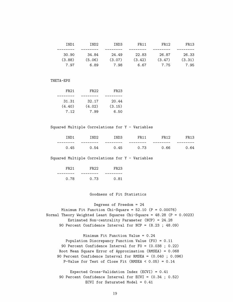
Error X Observed X Latent X Latent Y Observed Y Error Y

Figure 4.2: The Linear Structural Relations (LISREL) model integrates two measurementmodels with one regression model. How well are the X’s represented by the latent variables(factors) Xi, and how well are the Y variables represented by the factors etas.

12

22.51 29.54 20.61 57.61 78.9322.65 27.56 15.33 53.57 49.27 73.7633.24 46.49 31.44 67.81 54.76 54.58 141.7732.56 40.37 25.58 55.82 52.33 47.74 98.62 117.3330.32 40.44 27.69 54.78 53.44 59.52 96.95 84.87 106.35LAIND1 IND2 IND3 FR11 FR12 FR13 FR21 FR22 FR23MO NY=9 NE=3 PS=SY,FI TE=DI,FR LY=FU,FI BE=FU,FILEINDUCTN FIGREL1 FIGREL2FR LY(2, 1) LY(3, 1)FR LY(5, 2) LY(6, 2)FR LY(8, 3) LY(9, 3)VA 1 LY(1, 1) LY(4, 2) LY(7, 3)FR BE(2, 1) BE(3, 1) BE(3, 2)FR PS(1, 1) PS(2, 2) PS(3, 3)OU

This file is created (or in this case copied) and saved on the Mac/PC with a meaningfulname, rm5.txt, and then uploaded to the SSCC using a sftp operation. (From my MacI use Interarchy as my sftp client.)

3. submit the lisrel job by invoking lisrel8:

[revelle@hardin ~]$ lisrel8 rm5.txt rm5.out

+----------------------------------+| || L I S R E L 8.72 || || by || || Karl G. Joreskog and Dag Sorbom ||Available Workspace 16941056 bytes|+----------------------------------+This program is published exclusively byScientific Software International, Inc.7383 N.Lincoln Avenue - Suite 100Lincolnwood, IL 60712-1704, U.S.A.Phone: (800)247-6113, (847)675-0720, Fax: (847)675-2140Copyright by Scientific Software International, Inc., 1981-2005Use of this program is subject to the terms specified in theUniversal Copyright Convention.Website: www.ssicentral.comRevision LISREL872_03/28/2005Input file [INPUT] :Input file [INPUT] :rm5.txt

13

Output file [OUTPUT]:Output file [OUTPUT]:rm5.outReading input from file rm5.txt

STRUCTURAL REGRESSION MODELComputing Initial EstimatesComputing Information MatrixInverting Information MatrixIteration 1 for LISREL EstimatesIteration 2 for LISREL EstimatesIteration 3 for LISREL EstimatesIteration 4 for LISREL EstimatesIteration 5 for LISREL EstimatesIteration 6 for LISREL EstimatesComputing Information MatrixInverting Information MatrixComputing Goodness of Fit Statistics

[revelle@hardin ~]$

4. Transfer the output file (in this case “rm5.out”) back to your host machine (using sftp).

5. Examine the output

DATE: 2/12/2007TIME: 11:14

L I S R E L 8.72

BY

Karl G. J~Aoreskog & Dag S~Aorbom

This program is published exclusively byScientific Software International, Inc.

7383 N. Lincoln Avenue, Suite 100Lincolnwood, IL 60712, U.S.A.

Phone: (800)247-6113, (847)675-0720, Fax: (847)675-2140Copyright by Scientific Software International, Inc., 1981-2005Use of this program is subject to the terms specified in the

Universal Copyright Convention.Website: www.ssicentral.com

The following lines were read from file rm5.txt:

14

STRUCTURAL REGRESSION MODELDA NI=9 NO=220CM56.2131.55 75.5523.27 28.30 44.4524.48 32.24 22.56 84.6422.51 29.54 20.61 57.61 78.9322.65 27.56 15.33 53.57 49.27 73.7633.24 46.49 31.44 67.81 54.76 54.58 141.7732.56 40.37 25.58 55.82 52.33 47.74 98.62 117.3330.32 40.44 27.69 54.78 53.44 59.52 96.95 84.87 106.35LAIND1 IND2 IND3 FR11 FR12 FR13 FR21 FR22 FR23MO NY=9 NE=3 PS=SY,FI TE=DI,FR LY=FU,FI BE=FU,FILEINDUCTN FIGREL1 FIGREL2FR LY(2, 1) LY(3, 1)FR LY(5, 2) LY(6, 2)FR LY(8, 3) LY(9, 3)VA 1 LY(1, 1) LY(4, 2) LY(7, 3)FR BE(2, 1) BE(3, 1) BE(3, 2)FR PS(1, 1) PS(2, 2) PS(3, 3)OU

STRUCTURAL REGRESSION MODEL

Number of Input Variables 9Number of Y - Variables 9Number of X - Variables 0Number of ETA - Variables 3Number of KSI - Variables 0Number of Observations 220


Covariance Matrix

IND1 IND2 IND3 FR11 FR12 FR13-------- -------- -------- -------- -------- --------

IND1 56.21IND2 31.55 75.55IND3 23.27 28.30 44.45FR11 24.48 32.24 22.56 84.64FR12 22.51 29.54 20.61 57.61 78.93FR13 22.65 27.56 15.33 53.57 49.27 73.76

15

FR21 33.24 46.49 31.44 67.81 54.76 54.58FR22 32.56 40.37 25.58 55.82 52.33 47.74FR23 30.32 40.44 27.69 54.78 53.44 59.52

Covariance Matrix

FR21 FR22 FR23-------- -------- --------

FR21 141.77FR22 98.62 117.33FR23 96.95 84.87 106.35


Parameter Specifications

LAMBDA-Y

INDUCTN FIGREL1 FIGREL2-------- -------- --------

IND1 0 0 0IND2 1 0 0IND3 2 0 0FR11 0 0 0FR12 0 3 0FR13 0 4 0FR21 0 0 0FR22 0 0 5FR23 0 0 6

BETA


INDUCTN 0 0 0FIGREL1 7 0 0FIGREL2 8 9 0

PSI


10 11 12

THETA-EPS

16


13 14 15 16 17 18

THETA-EPS

FR21 FR22 FR23-------- -------- --------

19 20 21


Number of Iterations = 5

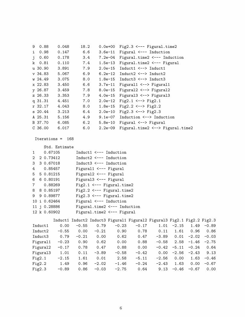
LISREL Estimates (Maximum Likelihood)

LAMBDA-Y


IND1 1.00 - - - -

IND2 1.27 - - - -(0.16)8.08

IND3 0.89 - - - -(0.12)7.70

FR11 - - 1.00 - -

FR12 - - 0.92 - -(0.07)13.76

FR13 - - 0.88 - -(0.06)13.54

FR21 - - - - 1.00

FR22 - - - - 0.88(0.05)16.79

17

FR23 - - - - 0.88(0.05)18.39

BETA


INDUCTN - - - - - -

FIGREL1 0.98 - - - -(0.15)6.64

FIGREL2 0.60 0.81 - -(0.18) (0.11)3.41 7.40

Covariance Matrix of ETA


INDUCTN 25.31FIGREL1 24.71 61.81FIGREL2 35.39 65.23 110.46

PSINote: This matrix is diagonal.


25.31 37.69 36.00(5.14) (6.10) (5.92)4.92 6.18 6.08

Squared Multiple Correlations for Structural Equations


- - 0.39 0.67

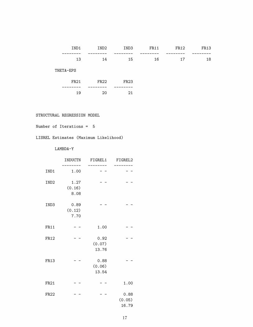
THETA-EPS

18


30.90 34.84 24.49 22.83 26.87 26.33(3.88) (5.06) (3.07) (3.42) (3.47) (3.31)7.97 6.89 7.98 6.67 7.75 7.95

THETA-EPS

FR21 FR22 FR23-------- -------- --------

31.31 32.17 20.44(4.40) (4.02) (3.15)7.12 7.99 6.50

Squared Multiple Correlations for Y - Variables


0.45 0.54 0.45 0.73 0.66 0.64


FR21 FR22 FR23-------- -------- --------

0.78 0.73 0.81

Goodness of Fit Statistics

Degrees of Freedom = 24Minimum Fit Function Chi-Square = 52.10 (P = 0.00076)

Normal Theory Weighted Least Squares Chi-Square = 48.28 (P = 0.0023)Estimated Non-centrality Parameter (NCP) = 24.28

90 Percent Confidence Interval for NCP = (8.23 ; 48.09)

Minimum Fit Function Value = 0.24Population Discrepancy Function Value (F0) = 0.11

90 Percent Confidence Interval for F0 = (0.038 ; 0.22)Root Mean Square Error of Approximation (RMSEA) = 0.06890 Percent Confidence Interval for RMSEA = (0.040 ; 0.096)

P-Value for Test of Close Fit (RMSEA < 0.05) = 0.14

Expected Cross-Validation Index (ECVI) = 0.4190 Percent Confidence Interval for ECVI = (0.34 ; 0.52)

ECVI for Saturated Model = 0.41

19

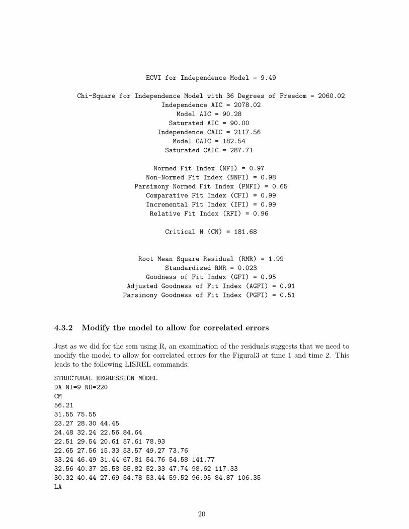
ECVI for Independence Model = 9.49

Chi-Square for Independence Model with 36 Degrees of Freedom = 2060.02Independence AIC = 2078.02

Model AIC = 90.28Saturated AIC = 90.00

Independence CAIC = 2117.56Model CAIC = 182.54

Saturated CAIC = 287.71

Normed Fit Index (NFI) = 0.97Non-Normed Fit Index (NNFI) = 0.98

Parsimony Normed Fit Index (PNFI) = 0.65Comparative Fit Index (CFI) = 0.99Incremental Fit Index (IFI) = 0.99Relative Fit Index (RFI) = 0.96

Critical N (CN) = 181.68

Root Mean Square Residual (RMR) = 1.99Standardized RMR = 0.023

Goodness of Fit Index (GFI) = 0.95Adjusted Goodness of Fit Index (AGFI) = 0.91Parsimony Goodness of Fit Index (PGFI) = 0.51

4.3.2 Modify the model to allow for correlated errors

Just as we did for the sem using R, an examination of the residuals suggests that we need tomodify the model to allow for correlated errors for the Figural3 at time 1 and time 2. Thisleads to the following LISREL commands:

STRUCTURAL REGRESSION MODELDA NI=9 NO=220CM56.2131.55 75.5523.27 28.30 44.4524.48 32.24 22.56 84.6422.51 29.54 20.61 57.61 78.9322.65 27.56 15.33 53.57 49.27 73.7633.24 46.49 31.44 67.81 54.76 54.58 141.7732.56 40.37 25.58 55.82 52.33 47.74 98.62 117.3330.32 40.44 27.69 54.78 53.44 59.52 96.95 84.87 106.35LA

20

IND1 IND2 IND3 FR11 FR12 FR13 FR21 FR22 FR23MO NY=9 NE=3 PS=SY,FI TE=SY,FI LY=FU,FI BE=FU,FILEINDUCTN FIGREL1 FIGREL2FR LY(2, 1) LY(3, 1)FR LY(5, 2) LY(6, 2)FR LY(8, 3) LY(9, 3)VA 1 LY(1, 1) LY(4, 2) LY(7, 3)FR BE(2, 1) BE(3, 1) BE(3, 2)FR PS(1, 1) PS(2, 2) PS(3, 3)FR TE(1,1) TE (2,2) TE(3,3) TE(4,4) TE(5,5) TE(6,6) TE(7,7) TE(8,8) TE(9,9) TE(9,6)OU

Compare this set of commands to the previous set. What we have done is added a line tospecify the errors in the “theta” matrix and specified that the 6th error correlates with the9th error.

Uploading this revised command file to the SSCC and running it leads to the followingoutput:

DATE: 2/12/2007TIME: 11:37

L I S R E L 8.72

BY

Karl G. J~Aoreskog & Dag S~Aorbom

This program is published exclusively byScientific Software International, Inc.

7383 N. Lincoln Avenue, Suite 100Lincolnwood, IL 60712, U.S.A.

Phone: (800)247-6113, (847)675-0720, Fax: (847)675-2140Copyright by Scientific Software International, Inc., 1981-2005Use of this program is subject to the terms specified in the

Universal Copyright Convention.Website: www.ssicentral.com

The following lines were read from file rm5a.txt:

STRUCTURAL REGRESSION MODELDA NI=9 NO=220CM

21

56.2131.55 75.5523.27 28.30 44.4524.48 32.24 22.56 84.6422.51 29.54 20.61 57.61 78.9322.65 27.56 15.33 53.57 49.27 73.7633.24 46.49 31.44 67.81 54.76 54.58 141.7732.56 40.37 25.58 55.82 52.33 47.74 98.62 117.3330.32 40.44 27.69 54.78 53.44 59.52 96.95 84.87 106.35LAIND1 IND2 IND3 FR11 FR12 FR13 FR21 FR22 FR23MO NY=9 NE=3 PS=SY,FI TE=SY,FI LY=FU,FI BE=FU,FILEINDUCTN FIGREL1 FIGREL2FR LY(2, 1) LY(3, 1)FR LY(5, 2) LY(6, 2)FR LY(8, 3) LY(9, 3)VA 1 LY(1, 1) LY(4, 2) LY(7, 3)FR BE(2, 1) BE(3, 1) BE(3, 2)FR PS(1, 1) PS(2, 2) PS(3, 3)FR TE(1,1) TE (2,2) TE(3,3) TE(4,4) TE(5,5) TE(6,6) TE(7,7) TE(8,8) TE(9,9) TE(9,6)OU


Number of Input Variables 9Number of Y - Variables 9Number of X - Variables 0Number of ETA - Variables 3Number of KSI - Variables 0Number of Observations 220


Covariance Matrix


IND1 56.21IND2 31.55 75.55IND3 23.27 28.30 44.45FR11 24.48 32.24 22.56 84.64FR12 22.51 29.54 20.61 57.61 78.93FR13 22.65 27.56 15.33 53.57 49.27 73.76FR21 33.24 46.49 31.44 67.81 54.76 54.58FR22 32.56 40.37 25.58 55.82 52.33 47.74FR23 30.32 40.44 27.69 54.78 53.44 59.52

22

Covariance Matrix

FR21 FR22 FR23-------- -------- --------

FR21 141.77FR22 98.62 117.33FR23 96.95 84.87 106.35


Parameter Specifications

LAMBDA-Y


IND1 0 0 0IND2 1 0 0IND3 2 0 0FR11 0 0 0FR12 0 3 0FR13 0 4 0FR21 0 0 0FR22 0 0 5FR23 0 0 6

BETA


INDUCTN 0 0 0FIGREL1 7 0 0FIGREL2 8 9 0

PSI


10 11 12

THETA-EPS


IND1 13

23

IND2 0 14IND3 0 0 15FR11 0 0 0 16FR12 0 0 0 0 17FR13 0 0 0 0 0 18FR21 0 0 0 0 0 0FR22 0 0 0 0 0 0FR23 0 0 0 0 0 21

THETA-EPS

FR21 FR22 FR23-------- -------- --------

FR21 19FR22 0 20FR23 0 0 22


Number of Iterations = 5

LISREL Estimates (Maximum Likelihood)

LAMBDA-Y


IND1 1.00 - - - -

IND2 1.27 - - - -(0.16)8.07

IND3 0.89 - - - -(0.12)7.71

FR11 - - 1.00 - -

FR12 - - 0.89 - -(0.06)13.89

FR13 - - 0.83 - -(0.06)

24

13.46

FR21 - - - - 1.00

FR22 - - - - 0.87(0.05)17.20

FR23 - - - - 0.86(0.05)18.39

BETA


INDUCTN - - - - - -

FIGREL1 1.00 - - - -(0.15)6.68

FIGREL2 0.67 0.75 - -(0.18) (0.11)3.74 7.10

Covariance Matrix of ETA


INDUCTN 25.17FIGREL1 25.13 64.97FIGREL2 35.70 65.51 112.37

PSINote: This matrix is diagonal.


25.17 39.88 39.37(5.13) (6.26) (6.05)4.91 6.37 6.51

Squared Multiple Correlations for Structural Equations

25


- - 0.39 0.65

THETA-EPS


IND1 31.04(3.88)8.00

IND2 - - 34.91(5.05)6.91

IND3 - - - - 24.32(3.06)7.95

FR11 - - - - - - 19.67(3.35)5.87

FR12 - - - - - - - - 27.71(3.53)7.84

FR13 - - - - - - - - - - 28.54(3.46)8.24

FR21 - - - - - - - - - - - -

FR22 - - - - - - - - - - - -

FR23 - - - - - - - - - - 12.26(2.46)4.99

THETA-EPS

FR21 FR22 FR23-------- -------- --------

FR21 29.40

26

(4.28)6.87

FR22 - - 31.34(3.95)7.93

FR23 - - - - 22.50(3.28)6.86



0.45 0.54 0.45 0.77 0.65 0.61


FR21 FR22 FR23-------- -------- --------

0.79 0.73 0.79

Goodness of Fit Statistics

Degrees of Freedom = 23Minimum Fit Function Chi-Square = 20.55 (P = 0.61)

Normal Theory Weighted Least Squares Chi-Square = 20.01 (P = 0.64)Estimated Non-centrality Parameter (NCP) = 0.0

90 Percent Confidence Interval for NCP = (0.0 ; 11.11)

Minimum Fit Function Value = 0.094Population Discrepancy Function Value (F0) = 0.0

90 Percent Confidence Interval for F0 = (0.0 ; 0.051)Root Mean Square Error of Approximation (RMSEA) = 0.090 Percent Confidence Interval for RMSEA = (0.0 ; 0.047)P-Value for Test of Close Fit (RMSEA < 0.05) = 0.96

Expected Cross-Validation Index (ECVI) = 0.3190 Percent Confidence Interval for ECVI = (0.31 ; 0.36)

ECVI for Saturated Model = 0.41ECVI for Independence Model = 9.49

Chi-Square for Independence Model with 36 Degrees of Freedom = 2060.02Independence AIC = 2078.02

27

Model AIC = 64.01Saturated AIC = 90.00

Independence CAIC = 2117.56Model CAIC = 160.67

Saturated CAIC = 287.71

Normed Fit Index (NFI) = 0.99Non-Normed Fit Index (NNFI) = 1.00

Parsimony Normed Fit Index (PNFI) = 0.63Comparative Fit Index (CFI) = 1.00Incremental Fit Index (IFI) = 1.00Relative Fit Index (RFI) = 0.98

Critical N (CN) = 444.69

Root Mean Square Residual (RMR) = 1.27Standardized RMR = 0.016

Goodness of Fit Index (GFI) = 0.98Adjusted Goodness of Fit Index (AGFI) = 0.96Parsimony Goodness of Fit Index (PGFI) = 0.50

4.4 Comparing the R and LISREL output

Each sem author has his or her own preferences about how to organize the output. Comparethe LISREL output 4.3.2 with the R output for the prediction model 4.2.3 and the correlationmodel 4.2.4.

As one would hope, the chi square values and df are equal between the two programs. LISRELgives far more goodness of fit statistics and also has a more detailed output than sem.

4.5 Testing for factorial invariance

The models tested above measured Figural Relations in the Junior and Senior year. Werethese tests measuring the same concept? If they were, then we would expect the factor loadingsto be the same in both years. We can test this by constraining the equivalent loadings to beidentical and comparing the differences in χ2 for the two models. (The first model is discussedin section4.2.3

path label initial estimate[1,] "Induction -> Induct1" NA "1"[2,] "Induction -> Induct2" "2" NA[3,] "Induction -> Induct3" "3" NA[4,] "Figural -> Figural1" NA "1"

28

[5,] "Figural -> Figural2" "5" NA[6,] "Figural -> Figural3" "6" NA[7,] "Figural.time2 -> Fig2.1" NA "1"[8,] "Figural.time2 -> Fig2.2" "5" NA[9,] "Figural.time2 -> Fig2.3" "6" NA[10,] "Induction -> Figural" "i" NA[11,] "Induction -> Figural.time2" "j" NA[12,] "Figural -> Figural.time2" "k" NA[13,] "Figural3 <-> Fig2.3" "10" NA[14,] "Induct1 <-> Induct1" "u" NA[15,] "Induct2 <-> Induct2" "v" NA[16,] "Induct3 <-> Induct3" "w" NA[17,] "Figural1 <-> Figural1" "x" NA[18,] "Figural2 <-> Figural2" "y" NA[19,] "Figural3 <-> Figural3" "z" NA[20,] "Fig2.1 <-> Fig2.1" "q" NA[21,] "Fig2.2 <-> Fig2.2" "r" NA[22,] "Fig2.3 <-> Fig2.3" "s" NA[23,] "Induction <-> Induction" "A" "1"[24,] "Figural <-> Figural" "B" "1"[25,] "Figural.time2 <-> Figural.time2" "C" "1"

Model Chisquare = 21 Df = 25 Pr(>Chisq) = 0.7Chisquare (null model) = 1177 Df = 36Goodness-of-fit index = 0.98Adjusted goodness-of-fit index = 0.96RMSEA index = 0 90% CI: (NA, 0.043)Bentler-Bonnett NFI = 0.98Tucker-Lewis NNFI = 1Bentler CFI = 1BIC = -114


-9.1e-01 -1.1e-01 4.9e-05 -1.1e-02 1.7e-01 6.0e-01


2 1.27 0.159 8.0 1.1e-15 Induct2 <--- Induction3 0.89 0.115 7.8 6.9e-15 Induct3 <--- Induction5 0.88 0.040 21.8 0.0e+00 Figural2 <--- Figural6 0.86 0.042 20.5 0.0e+00 Figural3 <--- Figurali 0.99 0.147 6.8 1.3e-11 Figural <--- Inductionj 0.67 0.181 3.7 2.0e-04 Figural.time2 <--- Inductionk 0.76 0.100 7.6 2.7e-14 Figural.time2 <--- Figural10 12.23 2.481 4.9 8.3e-07 Fig2.3 <--> Figural3u 31.03 3.891 8.0 1.6e-15 Induct1 <--> Induct1

29

v 34.90 5.060 6.9 5.3e-12 Induct2 <--> Induct2w 24.34 3.069 7.9 2.2e-15 Induct3 <--> Induct3x 19.85 3.234 6.1 8.3e-10 Figural1 <--> Figural1y 28.00 3.461 8.1 6.7e-16 Figural2 <--> Figural2z 28.19 3.417 8.2 2.2e-16 Figural3 <--> Figural3q 29.21 4.243 6.9 5.9e-12 Fig2.1 <--> Fig2.1r 31.14 3.917 8.0 1.8e-15 Fig2.2 <--> Fig2.2s 22.74 3.275 6.9 3.8e-12 Fig2.3 <--> Fig2.3A 25.18 5.141 4.9 9.7e-07 Induction <--> InductionB 39.43 5.833 6.8 1.4e-11 Figural <--> FiguralC 39.62 5.962 6.6 3.0e-11 Figural.time2 <--> Figural.time2

Iterations = 162


Induct1 Induct2 Induct3 Figural1 Figural2 Figural3 Fig2.1 Fig2.2 Fig2.3Induct1 0.00 -0.44 0.77 -0.48 0.56 1.29 -2.65 1.01 -0.38Induct2 -0.44 0.00 -0.29 0.52 1.66 0.42 0.89 0.28 1.43Induct3 0.77 -0.29 0.00 0.25 1.00 -3.76 -0.64 -2.62 0.25Figural1 -0.48 0.52 0.25 0.61 1.19 -1.33 2.33 -1.74 -1.24Figural2 0.56 1.66 1.00 1.19 1.33 1.01 -2.80 1.73 4.20Figural3 1.29 0.42 -3.76 -1.33 1.01 -1.40 -1.44 -1.50 -0.62Fig2.1 -2.65 0.89 -0.64 2.33 -2.80 -1.44 -0.89 -1.11 -0.10Fig2.2 1.01 0.28 -2.62 -1.74 1.73 -1.50 -1.11 -1.49 -0.45Fig2.3 -0.38 1.43 0.25 -1.24 4.20 -0.62 -0.10 -0.45 0.58

The difference in χ2 is trivial and we have gained two degrees of freedom. This suggests thatthe two measures are factorially equivalent.

4.5.1 Testing for factorial equivalence in multiple groups

Not shown in this chapter is how to test for equivalence of measurement across differentgroups. This involves best fitting the model for multiple groups simultaneously and will bediscussed in the next section (as yet unwritten).

30

4.6 References

Barratt, P. (2007) Structural equation modeling: Adjudging model fit. Personality and Indi-vidual Differences, 815-824. (Available for NU accounts athttp://www.sciencedirect.com/science/journal/01918869

Fox (2006), ”Structural Equation Modeling With the sem Package in R.” Structural EquationModeling, 13:465-486.

Rakov, T. & Marcoulides, G.A. (2006), A first course in structural equation modeling, 2ndEdition; Mawwah,N.J; Erlebaum

31

http://www.sciencedirect.com/science/journal/01918869

http://socserv.mcmaster.ca/jfox/Misc/sem/SEM-paper.pdf

Documents

Chapter 4: sem in R and in LISREL - Personality Project · code for many problems in LISREL and EQS syntax, Raykov and Marcoulides (2006) give examples in EQS, LISREL and Mplus. In