Chapter 4 Dynamics - frc.ri.cmu.edu · Chapter 4 Dynamics Part 2 ... 22 Mobile Robotics - Prof Alonzo Kelly, CMU RI ... • Using elimination, the solution is:

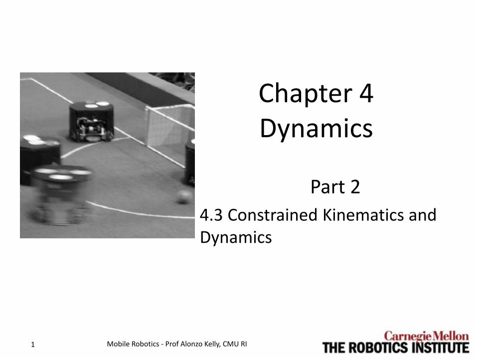
Chapter 4 Dynamics

Part 2 4.3 Constrained Kinematics and Dynamics

Mobile Robotics - Prof Alonzo Kelly, CMU RI 1

Outline • 4.3 Constrained Kinematics and Dynamics

– 4.3.1 Constraints of Disallowed Direction – 4.3.2 Constraints of Rolling without Slipping – 4.3.3 Lagrangian Dynamics – 4.3.4 Terrain Contact – 4.3.5 Trajectory Estimation and Prediction – Summary

2 Mobile Robotics - Prof Alonzo Kelly, CMU RI

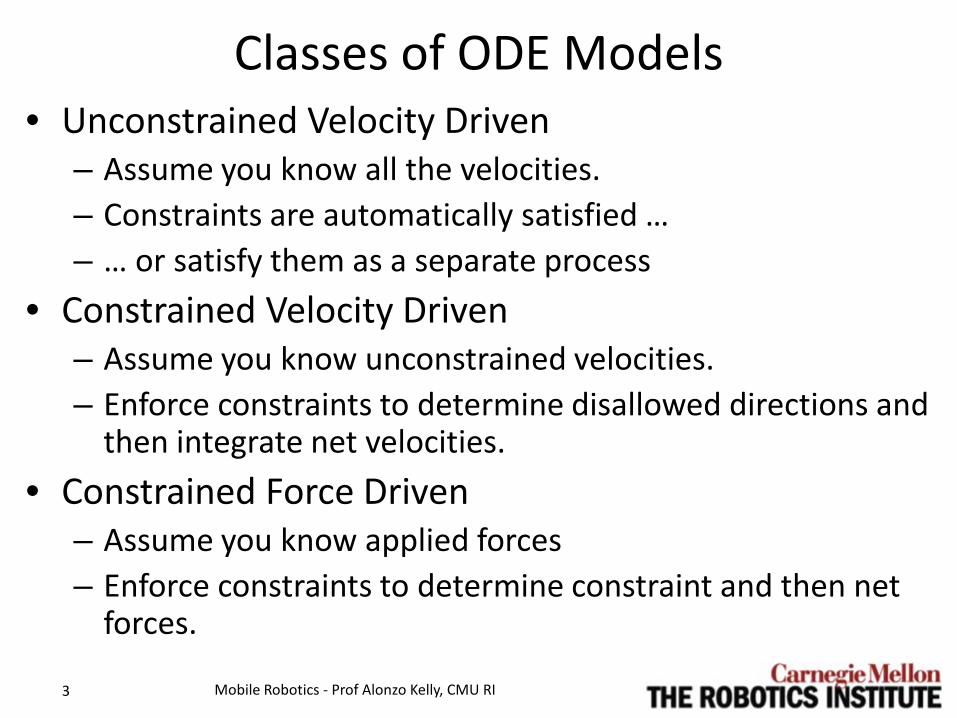
Classes of ODE Models • Unconstrained Velocity Driven

– Assume you know all the velocities. – Constraints are automatically satisfied … – … or satisfy them as a separate process

• Constrained Velocity Driven – Assume you know unconstrained velocities. – Enforce constraints to determine disallowed directions and

then integrate net velocities. • Constrained Force Driven

– Assume you know applied forces – Enforce constraints to determine constraint and then net

forces. Mobile Robotics - Prof Alonzo Kelly, CMU RI 3

What’s the Big Deal with Dynamics? • “Its all just F = ma integrated twice” Right? • Well, what is f1, f2, r1,and r2?

• What about T = I α ? What are all the torques caused by the wheels?


𝑚𝑚𝑚𝑚 𝑟𝑟1 𝑟𝑟2 𝑓𝑓2 𝑓𝑓1

Dynamics of WMR • Two constraints:

– Rolling without sliding – Terrain contact

• Two Formulations – Second Kind: Lagrangian formulation of dynamics

computes the constraint forces automatically. • Few (generalized) coordinates. Complex nonlinear equations.

– First Kind: Augmented formulation leaves them explicit. • All coordinates. Simple linear equations. • Lets you determine if the terrain can provide the forces. • We will do this kind.


4.3 Constrained WMR Models • The “constraints” were not explicit in the last

section. – Actually, they were, wheel equations are constraints

too.

• Constrained models occur in both control and estimation contexts.

• Non slip constraints are nonholonomic, of abstract form:

• Terrain contact constraints are holonomic, of abstract form: Mobile Robotics - Prof Alonzo Kelly, CMU RI 6




Differentiating Holonomic Constraints • If we differentiate a holonomic constraint:

• We get a form that resembles Pfaffian form:

• Where the constraint gradient 𝑐𝑐𝑥𝑥 functions just

like a disallowed direction of motion. • This is convenient but this differentiated

constraint can still be integrated so the constraint is still holonomic.


Expressing Wheel Constraints • It is trivial to write an expression that says a wheel

cannot move sideways. • The implementation issue is how does a set of

such statements constrain the motion of the body frame of the vehicle.

• We solve this problem by substituting the kinematics into the constraint: – Replace wheel velocity with body velocity.


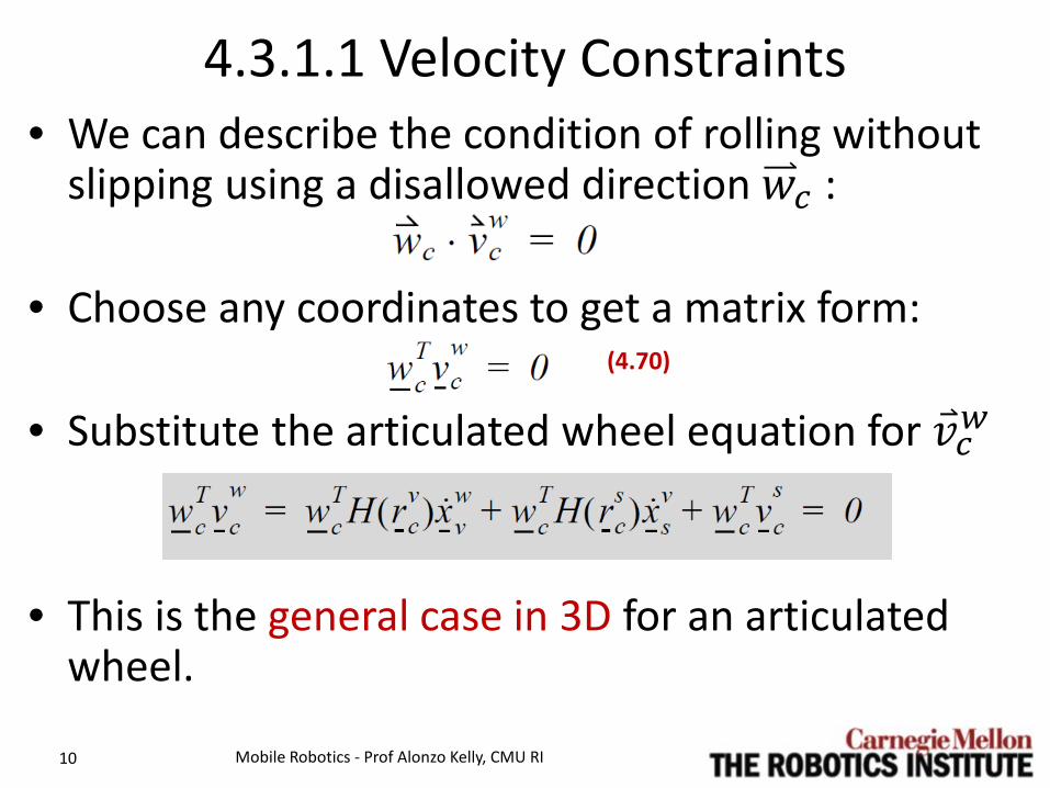
4.3.1.1 Velocity Constraints • We can describe the condition of rolling without

slipping using a disallowed direction 𝑤𝑤𝑐𝑐 :

• Choose any coordinates to get a matrix form:

• Substitute the articulated wheel equation for 𝑣𝑣𝑐𝑐𝑤𝑤

• This is the general case in 3D for an articulated wheel.


(4.70)

4.3.1.1 Velocity Constraints (c fixed) • In the special case where the contact point is fixed, the

velocity reduces to the (nonoffset) wheel equation:

• Substituting this into the wheel constraint gives:

• Define a “Pfaffian radius” then:

• It says translational and rotational components must cancel in the disallowed direction.


(4.40) Wheel Equation

Wheel Constraint for c Fixed

(4.75)

4.3.1.2 Differentiated Velocity Constraints • Differentiate Eqn 4.70 wrt time: • Substitute the articulated wheel equation for 𝑣𝑣𝑐𝑐𝑤𝑤

and �⃑�𝑎𝑐𝑐𝑤𝑤.

• This is the general case in 3D for an articulated wheel.


(4.70)

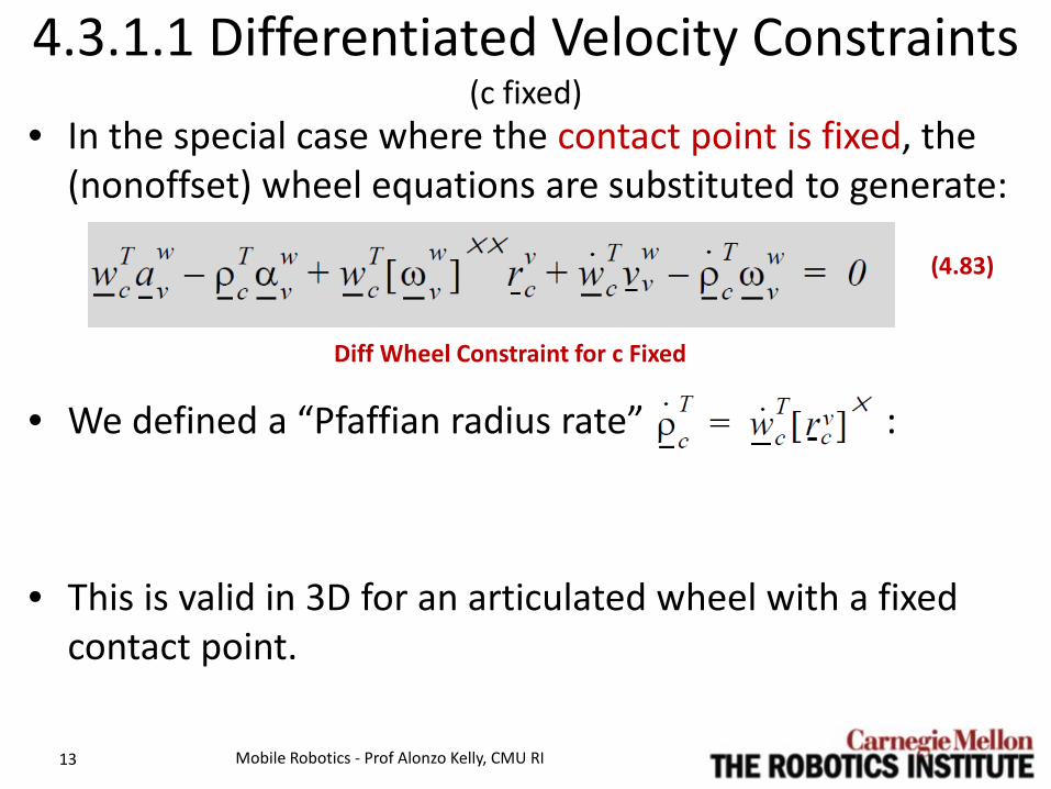
4.3.1.1 Differentiated Velocity Constraints (c fixed)

• In the special case where the contact point is fixed, the (nonoffset) wheel equations are substituted to generate:

• We defined a “Pfaffian radius rate” :

• This is valid in 3D for an articulated wheel with a fixed contact point.


Diff Wheel Constraint for c Fixed

(4.83)

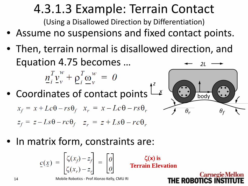
4.3.1.3 Example: Terrain Contact (Using a Disallowed Direction by Differentiation)

• Assume no suspensions and fixed contact points. • Then, terrain normal is disallowed direction, and

Equation 4.75 becomes …

• Coordinates of contact points

• In matrix form, constraints are:


ζ(x) is Terrain Elevation

2L

𝜃𝜃𝑟𝑟 𝜃𝜃𝑓𝑓

x z

body

4.3.1.3 Example: Terrain Contact • Constraint Jacobian:

• Suppose L=1; θ=0 ; slopes as shown:

• This can be verified by a more conventional technique.


cx0.1 1– 10.2– 1– 1–

=

x· I cxT cxcx

T( )1–cx–[ ]f x u,( ) 0.9268 0.0463– 0.1390–

T= =

2L

𝜃𝜃𝑟𝑟 𝜃𝜃𝑓𝑓

x z

body

Terrain Gradient




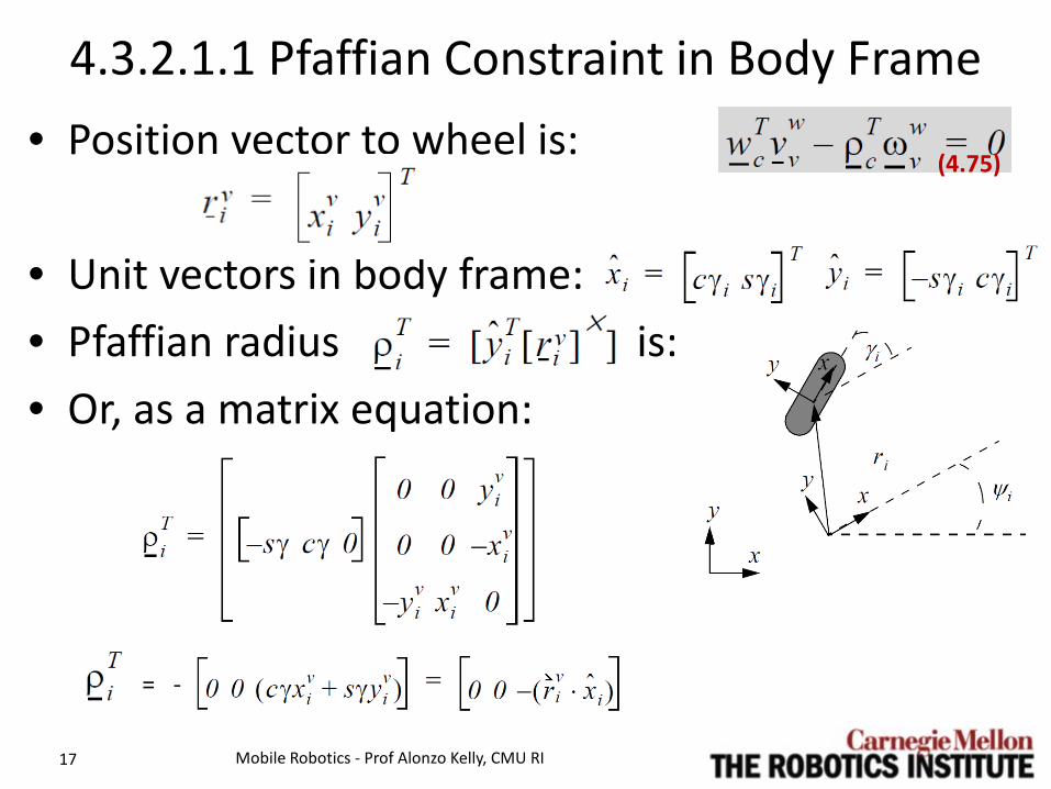
4.3.2.1.1 Pfaffian Constraint in Body Frame • Position vector to wheel is:

• Unit vectors in body frame: • Pfaffian radius is: • Or, as a matrix equation:


(4.75)

= -

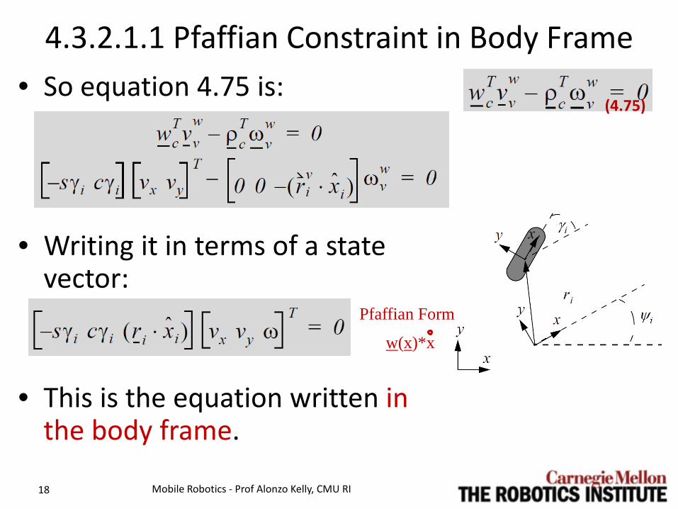
4.3.2.1.1 Pfaffian Constraint in Body Frame • So equation 4.75 is:

• Writing it in terms of a state

vector:

• This is the equation written in the body frame.


(4.75)

Pfaffian Form

w(x)*x

4.3.2.1.2 Pfaffian Constraint in Inertial Frame • Now the unit vectors are: • Writing it in terms of a state

vector:

• This is the equation written in the inertial frame.


(4.75)

(4.87)

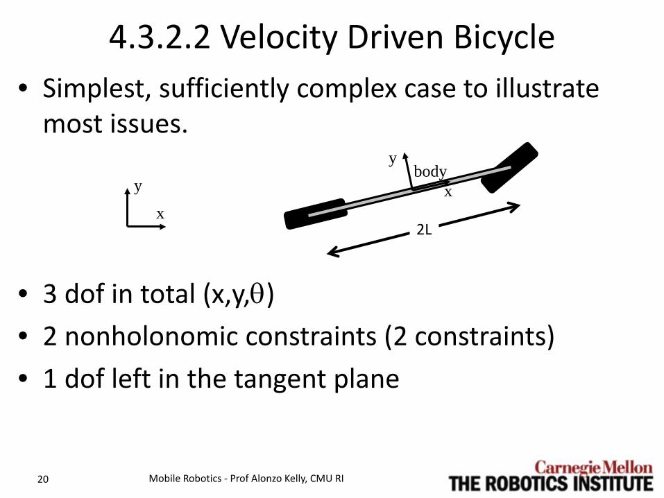
4.3.2.2 Velocity Driven Bicycle • Simplest, sufficiently complex case to illustrate

most issues.

• 3 dof in total (x,y,θ) • 2 nonholonomic constraints (2 constraints) • 1 dof left in the tangent plane


x

y body

y

x

2L

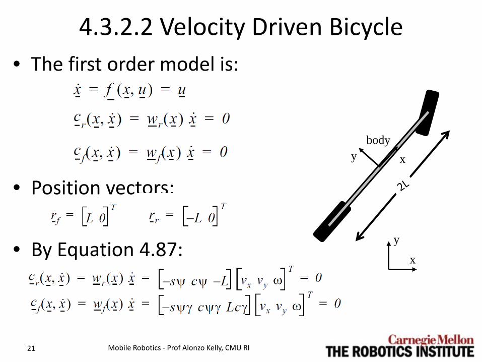
4.3.2.2 Velocity Driven Bicycle • The first order model is:

• Position vectors:

• By Equation 4.87:


x

y

body y x

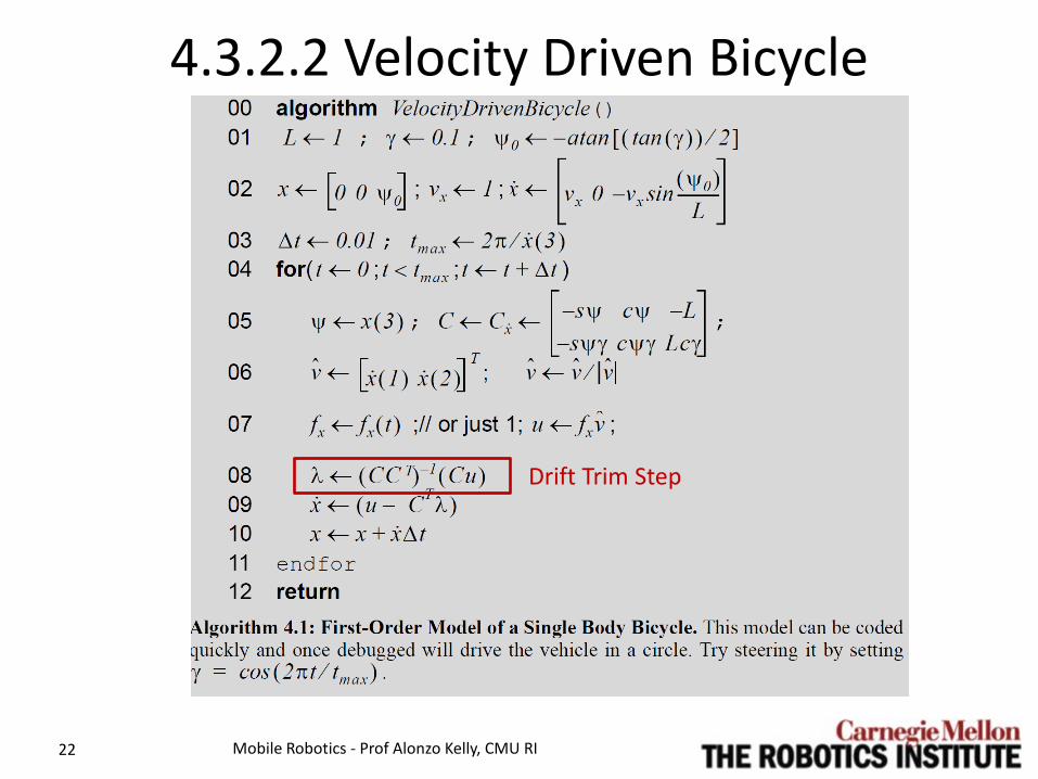
4.3.2.2 Velocity Driven Bicycle


Drift Trim Step

Demos : Unibody Bike





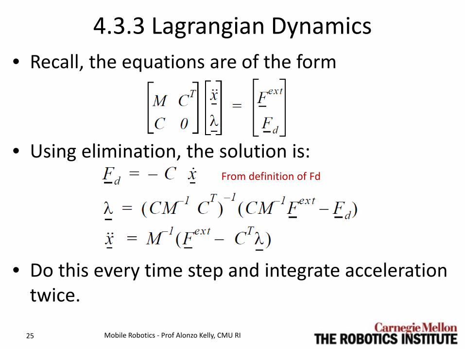
4.3.3 Lagrangian Dynamics • Recall, the equations are of the form

• Using elimination, the solution is:

• Do this every time step and integrate acceleration twice.


From definition of Fd

4.3.31 Differentiated Pfaffian Constraints (For a Wheel)

• Two key components of equation 4.83 are:

• After much manipulation:

• This is, by necessity, written in an inertial frame.


(4.83)

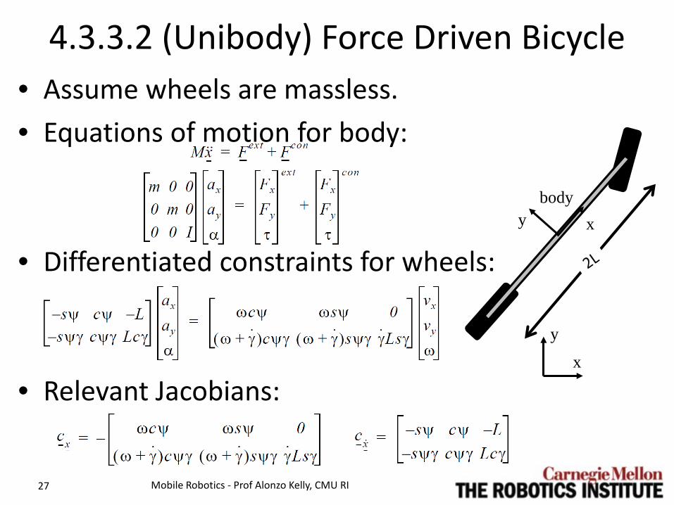
• Assume wheels are massless. • Equations of motion for body:

• Differentiated constraints for wheels:

• Relevant Jacobians:

4.3.3.2 (Unibody) Force Driven Bicycle


x

y

body y x

4.3.3.3 Force Driven Bicycle


Drift Trim Step

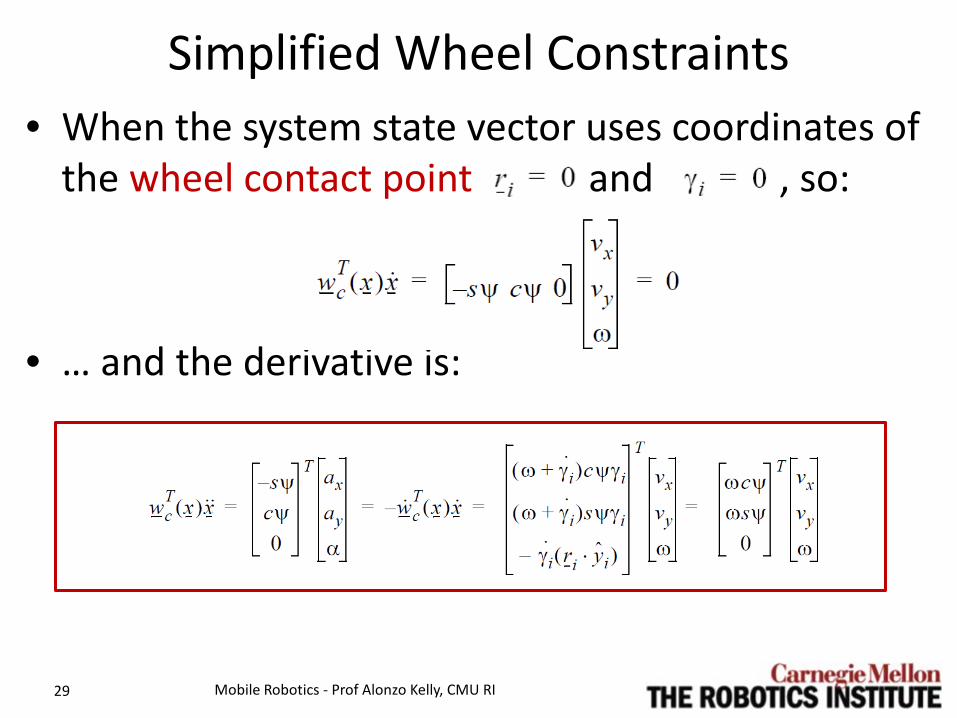
Simplified Wheel Constraints • When the system state vector uses coordinates of

the wheel contact point and , so:

• … and the derivative is:


(Multibody) Bicycle • Now have three bodies with mass.

• 9 dof in total: 3 X (x,y,q) • 1 rigidity constraint (3 constraints) • 1 rotary (steer) joint (2 constraints) • 2 nonholonomic constraints (2 constraints) • 2 dof left in tangent plane (steer, V)


x

y body

y

x

2L

Demos : 3 Body Bike


Other Issues • Allowing wheel slip according to a specific model. • Computing explicit constraint forces. • Inconsistent constraints. • Redundant constraints.





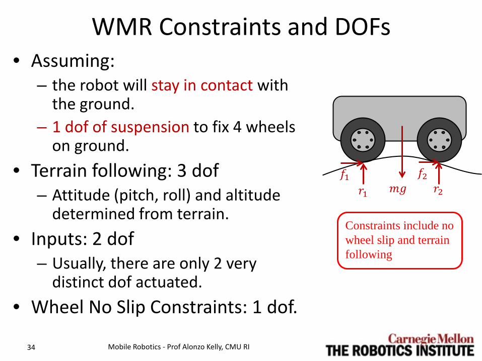
WMR Constraints and DOFs • Assuming:

– the robot will stay in contact with the ground.

– 1 dof of suspension to fix 4 wheels on ground.

• Terrain following: 3 dof – Attitude (pitch, roll) and altitude

determined from terrain. • Inputs: 2 dof

– Usually, there are only 2 very distinct dof actuated.

• Wheel No Slip Constraints: 1 dof.


Constraints include no wheel slip and terrain following

𝑚𝑚𝑚𝑚 𝑟𝑟1 𝑟𝑟2 𝑓𝑓2 𝑓𝑓1

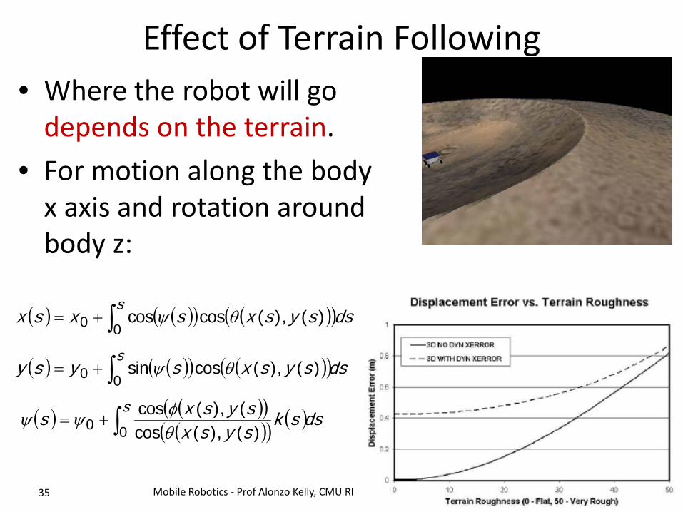
Effect of Terrain Following • Where the robot will go

depends on the terrain. • For motion along the body

x axis and rotation around body z:


( ) ( )( ) ( )( )dssysxsxsxs

)(),(coscos00 θψ∫+=

( ) ( )( ) ( )( )dssysxsysys

∫+=00 )(),(cossin θψ

( ) ( )( )( )( ) ( )dssk

sysxsysxs

s∫+=00 )(),(cos

(),(cosθφψψ

Basic Terrain Following • Start with known (x,y,z) from DE:

• Simple but not so accurate.


1 2

3 4

W

L

θlef t z1 z3–( ) L⁄=zi terrain xi yi,( ) i∀=

θright z2 z4–( ) L⁄=

φf ront z1 z2–( ) W⁄=φback z3 z4–( ) W⁄=

θ θr ight θlef t+( ) 2⁄=

φ φf ront φback+( ) 2⁄=

wheels

4.3.4.1 Least Residual Terrain Following • Assumes no suspension. • Minimize total residual of wheel heights and

terrain elevations.

• Unconstrained optimization: Solve using nonlinear least squares.


Wheel position

𝜌𝜌

z4

z2

Terrain

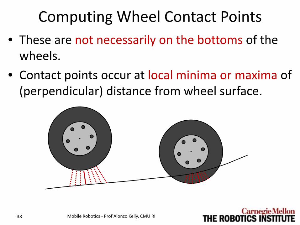
Computing Wheel Contact Points • These are not necessarily on the bottoms of the

wheels. • Contact points occur at local minima or maxima of

(perpendicular) distance from wheel surface.


• Let 𝑥𝑥 = 𝑥𝑥1 𝑥𝑥2 𝑥𝑥3 𝑥𝑥4 𝑇𝑇 … – represent spring deflections

• Spring forces are …

• Problem formulation

• Require suspension to be in minimum energy configuration.

Least Energy Terrain Following


kx1

kx2

mg

4 wheel contact constraints

Springs carry weight

Some Terrain Following Robots


CMU Rover prototype called Scarab used an averaging suspension that kept the bogy at the average pitch of the left and right halves.

EPFL rover SHRIMP uses four-bar mechanisms to achieve extended climbing capabilities.

The MER Rovers Spirit and Opportunity used a rocker-bogie design that was intended to keep the forces on all wheels roughly constant.




4.3.5 Trajectory Estimation and Prediction • Up to now, we have concentrated on how you

form the differential equation. • Next issue is how do you integrate it. • There are two purposes:

– For state estimation, especially odometry (inputs are measurements)

– For state prediction in predictive control (inputs are controls)

• Convenience of using body coordinates is now over. Must convert velocities to earth fixed frame to integrate.


4.3.5.1 Heading, Yaw and Curvature • Heading z is the angle of the path tangent. • Yaw y is the direction of the forward

looking axis • These may be related or unrelated on a

given vehicle. • Curvature is a property of the path. • Radius of curvature is its reciprocal. • By the chain rule:


ζ

ψ

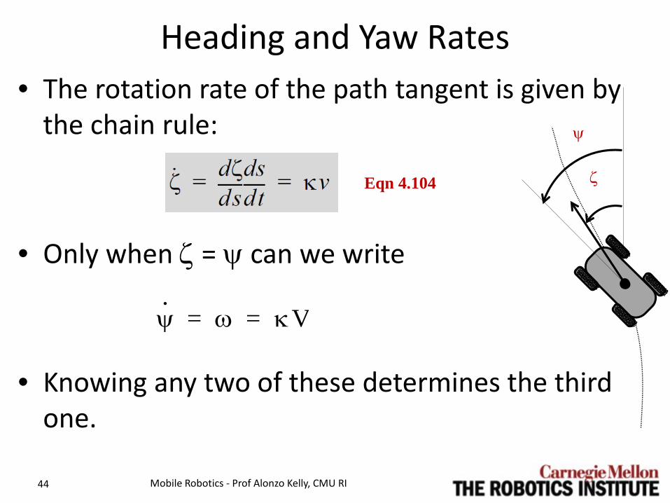
Heading and Yaw Rates • The rotation rate of the path tangent is given by

the chain rule:

• Only when ζ = ψ can we write

• Knowing any two of these determines the third one.


ψ· ω κV= =

ζ

ψ

Eqn 4.104

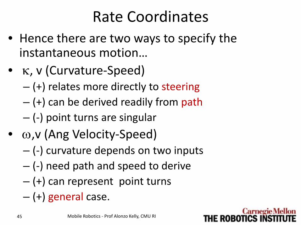
Rate Coordinates • Hence there are two ways to specify the

instantaneous motion… • κ, v (Curvature-Speed)

– (+) relates more directly to steering – (+) can be derived readily from path – (-) point turns are singular

• ω,v (Ang Velocity-Speed) – (-) curvature depends on two inputs – (-) need path and speed to derive – (+) can represent point turns – (+) general case.


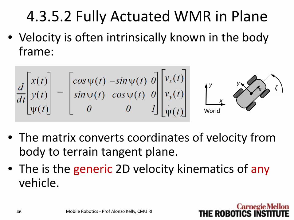
4.3.5.2 Fully Actuated WMR in Plane • Velocity is often intrinsically known in the body

frame:

• The matrix converts coordinates of velocity from

body to terrain tangent plane. • The is the generic 2D velocity kinematics of any

vehicle.


World

x

y y 𝜁𝜁 x

4.3.5.2 Fully Actuated WMR in Plane • If heading and yaw are the same (ζ = ψ ), lateral

velocity vanishes by definition:

• By assumption, the velocity vector is expressed in a frame aligned with the velocity vector.


4.3.5.3 UnderActuated WMR in Plane • If the vehicle frame is at center of rear wheels of a

car then ζ = ψ. Substitute Eqn 1.104 into last result:

• Its integral is simply:


World

x

y y 𝜁𝜁 x

4.3.5.4 Fully Actuated WMR in 3D


Steering Dynamics

Delay

)(tuvκ

Throttle Dynamics

Delay

× Coordinate Transform ∫ dt

Coordinate Transform ∫ dt

Terrain Contact

)( τκ −tuv κ

vv

κ

βv

V

ωw

ψ

vw

[ ]Tz φθ

[ ]Tyx

[ ]Tw zyxp =

κ

ψvv

)( τ−tuvv

)(tuvv

Since any vehicle has a curvature and speed, this is quite general

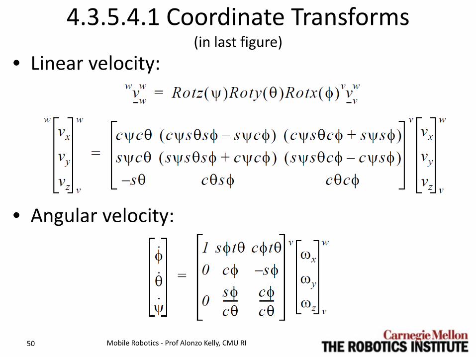
4.3.5.4.1 Coordinate Transforms (in last figure)

• Linear velocity:

• Angular velocity:


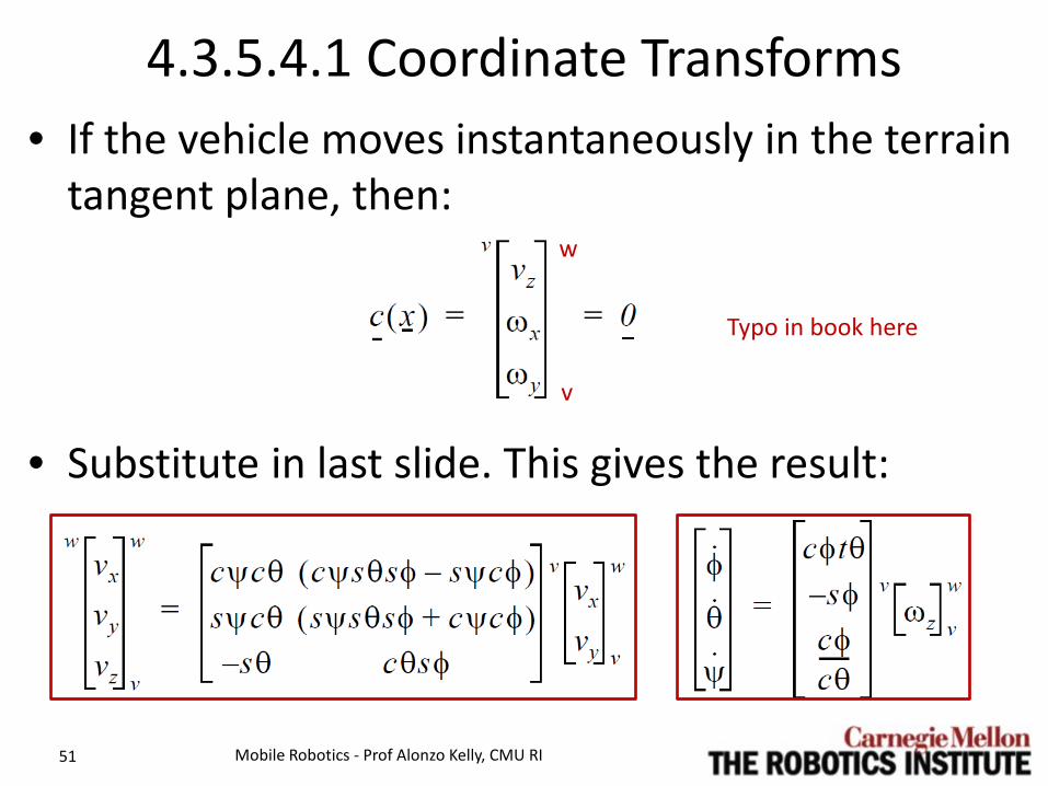
4.3.5.4.1 Coordinate Transforms • If the vehicle moves instantaneously in the terrain

tangent plane, then:

• Substitute in last slide. This gives the result:


v

w

Typo in book here




Summary • Disallowed Directions of Motion:

– Terrain following is a holonomic constraint but it can be written in a form that uses a disallowed direction.

– Wheel slip constraints are nonholonomic and use a disallowed direction

– The difference is that the first direction is fixed in the world frame and the second in the vehicle frame.

• WMR Kinematics and WMR (Lagrangian) Dynamics can both be formulated as constrained differential equations.

• Terrain contract can also be formulated as an energy minimization problem.

• Trajectory estimation and prediction require a conversion of body velocities to world coordinates and integration wrt time. Mobile Robotics - Prof Alonzo Kelly, CMU RI 53

Documents

Chapter 4 Dynamics - frc.ri.cmu.edu · Chapter 4 Dynamics Part 2 ... 22 Mobile Robotics - Prof Alonzo Kelly, CMU RI ... • Using elimination, the solution is: