39

Chapter 4

Convex Optimization

At the conclusion of chapter 3, we suggested that a natural question to ask is whether

Tikhonov regularization is really the best choice for the purpose of the inverse pho-

tonic problem. We learned that regularization is a way to impose additional con-

straints on an under-determined (rank-deficient) system so that an ill-posed problem

becomes well-posed. Therefore, given an actual physical problem, one ought to be

able to customize a more appropriate set of constraints based on the relevant physics.

Suppose the desired solution has a fairly sizeable norm. Under Tikhonov, is there

a possibility that we might ‘regularize out’ valid solutions because the norm con-

straint is not sophisticated enough? For an even worse effect, given our application,

a solution with negative values would still have a small norm, but in the case of pho-

tonic materials, the solution (representing the dielectric function) would not even be

feasible. More succinctly, requiring a small norm does not correlate with valid and

desirable photonic device designs. A more suitable approach places upper and lower

bounds on the value of the dielectric function that correspond to air and semiconduc-

tor. We will derive in chapter 6 the inverse photonic problem, but for now, consider

the regularized problem given these constraints of the form:

minη|Aη − b|2

subject to ηmin ¹ F−1η ¹ ηmax

(4.1)

40

where F−1 is the inverse fourier transform operator. Equation (4.1) is a quadratic

minimization problem with linear inequality constraints, and falls under the general

category of convex optimization problems. Casting this problem in the form of a

convex optimization (CO) is powerful because rigorous bounds have been derived on

the optimality of their solutions [1] using interior point methods. Therefore, with the

only constraint being that the dielectric function take on physically realizable values,

we can prove rigorously whether any dielectric function exists that would support a

given target mode, as indicated by the magnitude of the residual norm. This chapter

is devoted to developing our implementation of the convex optimization algorithm.

4.1 Introduction

We have all encountered optimization problems, and our first exposure to them is

likely to have been in a calculus course. Given some function f(x) defined over some

interval x ∈ [a, b], find where the maximum (or minimum) value of f occurs along

that interval. In the language we will use below, we call x the ‘optimization variable,’

and f the ‘objective function.’ Restricting x on the interval [a, b] can be viewed as

an ‘inequality constraint’ on the optimization variable. We can locate local extrema

since they satisfy the following condition:

df

dx

∣∣∣∣xe

= 0 (4.2)

The sign of the second derivative evaluated at those points {xe} classifies the kind

of extremum (maximum, minimum, or inflection point) at those points. To find the

global optimum, we evaluate f at all the local extrema, plus the end points, and then

choose from among these the optimal value (x∗), and we call x∗ the solution to the

optimization problem1. For arbitrary functions, the problem becomes more difficult

as eqn. (4.2) may not have analytical solutions. Numerical optimization in 1D is

1Here we follow Boyd’s notation, and x∗ does not denote the complex conjugate of x. Boyd onlydeals with real-valued variables and functions, so the notation is fine. Later in this chapter whenwe deal with complex variables, we will use η to denote the complex conjugate of η.

41

relatively straightforward, as we can just plot the function and visually determine the

extremum points. However, the problem scales unfavorably as the dimensionality of

x increases.

minimize fo(x)

subject to fi(x) ≤ 0, i = 1, ..., m

gj(x) = 0, j = 1, ..., p

, (4.3)

where f0 : Rn → R is the objective function, x ∈ Rn is now an n-dimensional

optimization variable, and {fi : Rn → R} and {gi : Rn →R} define the m inequality

constraints and p equality constraints respectively that x must satisfy in order to be

a valid solution. We refer to any x that does not satisfy all the constraints as an

‘infeasible point.’ The problem of maximizing an objective function is achieved by

simply reversing its sign.

An optimization problem is called a ‘convex optimization’ problem if it satisfies

the extra requirement that f0 and {fi} are convex functions (which we will define

in the next section), and {gi} are affine functions. Furthermore, the set of feasible

points must also form a convex set. The special property for this class of problem is

that any local minimum is by definition also the global minimum, and thus solves the

optimization problem.

4.1.1 Organization

As with the simple one-dimensional variable optimization, we will find the first and

second derivatives play critical roles in these optimization algorithms, so we begin

with the definition of multidimensional derivatives in section 4.2. For our applica-

tion, we will need to extend the treatment to include the use of complex variables,

which have some minor complications we will address. We will formally define convex

functions in section 4.3 and discuss some of their properties, highlighting those that

help with understanding the optimization problem. With the mathematical tools suf-

ficiently developed, we can then explain how to implement the convex optimization

42

method in section 4.4. We explain how to select descent directions and the line search

routine for an unconstrained optimization first, and then show how constraints can

be incorporated. Again, our primary concern in the presentation here is not to be

mathematically rigorous, but rather make it accessible for engineers and physicists

looking for a softer entry point. With the exception of the modification required for

functions with complex variables, the material in this chapter is adapted from the

textbook by Boyd and Vandenberghe [1], where they provide a much more thorough

and rigorous treatment of convex optimization methods.

4.2 Derivatives

For a real-valued function f : Rn →R, the definition of the gradient is

∇f(x)i ≡ ∂f(x)

∂xi

, i = 1, . . . , n, (4.4)

provided that the partial derivatives evaluated at x exist, and where ∇f(x) is written

as a column vector. The first-order Taylor approximation of the function f near x is

f(y) ≈ f(x) +∇f(x)T (y − x) (4.5)

which is an affine function of y.

The second derivative of a real-valued function f : Rn → R is called a Hessian

matrix, denoted ∇2f(x), with the matrix elements given by:

∇2f(x)ij ≡ ∂2f(x)

∂xi∂xj

, i = 1, . . . , n, i = 1, . . . , n, (4.6)

provided that f is twice differentiable at x and the partial derivatives are evaluated

at x. The second-order Taylor approximation of the function f near x is

f(y) ≈ f(x) +∇f(x)T (y − x) +1

2(y − x)T∇2f(x)(y − x) (4.7)

43

We now derive some shorthand notation for taking derivatives of matrix equations

representing functions f : Rn →R.

For functions that are linear in x:

f(x) = aT x = xT a (4.8)

=∑

i

aixi (4.9)

∇f(x)i ≡ ∂f

∂xi

(4.10)

= ai (4.11)

∴ ∇f(x) = a. (4.12)

The Hessian is obviously 0 in this case.

For functions that are quadratic in x:

f(x) = xT Bx =∑i,j

xibijxj (4.13)

∇f(x)i ≡ ∂f

∂xi

(4.14)

= xT ∂Bx

∂xi

+∂xT

∂xi

Bx (4.15)

= xT [B]coli + eT

i

∑

k

bikxk (4.16)

=∑

k

(bki + bik)xk (4.17)

∇f(x) =(B + BT

)x, (4.18)

where [B]coli denotes the ith column of the matrix B and ei is ith basis-vector. For the

44

Hessian, we obtain

∇f(x)ij ≡ ∂2f

∂xi∂xj

(4.19)

=∂

∂xi

∇f(x)j (4.20)

=∂

∂xi

[(B + BT )x

]j

(4.21)

=∂

∂xi

∑i

(bji + bij)x (4.22)

= bji + bij (4.23)

∇2f(x) = B + BT . (4.24)

For composite functions of the form h(x) = g(f(x)) such that h : Rn → R, with

f : Rn →R, and g : R→ R, the chain rule for gradients is:

∇h(x) = g′(f(x))∇f(x). (4.25)

The chain rule for the Hessian is evaluated to:

∇2h(x) = g′(f(x))∇2f(x) + g′′(f(x))∇f(x)∇f(x)T . (4.26)

The chain rules will be very useful for incorporating the barrier functions to impose

inequality constraints.

4.2.1 Complex variables

For the photonic problem, the optimization variable η will in general be complex.

Therefore, our matrices and vectors will be complex as well. Our objective function

f(η) : Cn → R is actually the 2-norm of a complex residual |Aη− b|2. We have found

few resources that deal explicitly with complex derivatives. Petersen and Pedersen’s

reference [25] shows that we can treat η and η as independent variables, and then

the generalized complex gradient is found by taking the derivatives with respect to

45

η. This expression for the gradient is suitable for use with gradient descent methods.

∇f(η) ≡ 2∂f(η, η)

∂η(4.27)

For linear functions, we have

f(η) = 2|a†η| = a†η + η†a (4.28)

= a†η + ηT a (4.29)

∇f ≡ 2∂ηT a

∂η(4.30)

= 2a. (4.31)

For quadratic functions, we have

f(η) = η†A†Aη (4.32)

= ηT A†Aη (4.33)

∇f = 2A†Aη. (4.34)

The Hessian for the quadratic function is

∇2f(η) = 2A†A. (4.35)

Unfortunately, it turns out that we cannot define a chain rule for differentiating

complex variables. Part of the reason is that a real-valued function of a complex

variable is strictly not differentiable because it does not satisfy the Cauchy-Riemann

equations, which state for f(η) = f(x + iy) = u(x, y) + iv(x, y), where u, v are real

valued functions of the real variables x = <(η), y = =(η)

∂u(x, y)

∂x=

∂v(x, y)

∂y

∂u(x, y)

∂y= −∂v(x, y)

∂x

. (4.36)

46

A real valued function implies v = 0, so in order to satisfy Cauchy-Riemann u cannot

depend on x or y. The linear and quadratic functions happen to be special cases for

which these can be defined, but in general, we cannot evaluate complex gradients and

Hessians directly. However, we can treat <(η) and =(η) as independent real variables

so now we have a function f(x, y) : R2n → R. All of the previous and subsequent

results can now be applied, provided we define our functions in this form. We return

to our linear and quadratic matrix functions and see what the equivalent structure

looks like.

We define a Cn →R2n transformation for a complex column vector:

[η] → x

y

≡ [ξ]. (4.37)

The adjoint operation of the vector η → η† becomes ξ → ξT . This definition preserves

the norm of the vector.

η†η = ξT ξ (4.38)

(xT − iyT )(x + iy) = [xT yT ]

x

y

(4.39)

xT x + yT y = xT x + yT y (4.40)

∵ xT y = yT x (4.41)

For the function to be real-valued, vector-vector products must come in adjoint pairs,

i.e.,

η†1η2 + η†2η1 → [xT1 yT

1 ]

x2

y2

+ [xT

2 yT2 ]

x1

y1

(4.42)

i(η†1η2 − η†2η1) → [yT1 − xT

1 ]

x2

y2

− [yT

2 − xT2 ]

x1

y1

(4.43)

where we have used iη† = i(xT − iyT ) = yT − i(−xT ) in the second relation. We must

47

of course be cautious that if the function is not real-valued, this transformation breaks

down (e.g., a general dot product of 2 complex valued vectors will give a complex

number), so it is not accommodated here.

For matrix multiplications, we define the transformation A ∈ Cn×n → A ∈ R2n×2n

as follows:

[A] → Ar −Ai

Ai Ar

, (4.44)

where Ar = <(A), and Ai = =(A). As before, the Hermitian adjoint becomes the

simple transpose operation. Matrix-vector multiplications are preserved:

Aη = Aξ (4.45)

(Ar + iAi)(x + iy) =

Ar −Ai

Ai Ar

x

y

(4.46)

(Arx− Aiy) + i (Aix + Ary) =

Arx− Aiy

Aix + Ary

. (4.47)

In appendix B, we will show that using the chain rule for the log barrier function

with the generalized complex gradient definition is incompatible with our definition

here for a simple linear constraint function. For the remainder of the thesis, we will

not explicitly write out the conformal mapping from Cn to R2n.

4.3 Convex Sets and Functions

A set SC is convex if the line segment between any two members of the set x1 and

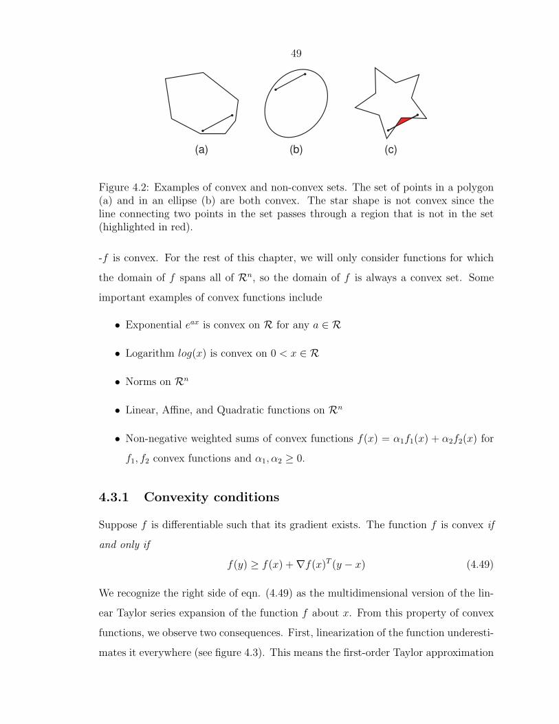
x2 also lies in SC . The geometric representation is shown in figure 4.2. Important

examples of convex sets are hyperplanes which have the form {x|aT x = b} and half-

spaces {x|aT x < b}, where a ∈ Rn, a 6= 0, and b ∈ R. Other common convex

sets include spheres, cones, and polyhedra. The set defined by the intersection of

two convex sets is also convex, so intersection preserves convexity. This is important

in our definition of a convex optimization problem, since as long as our constraint

48

-5 0 5-5

-4

-3

-2

-1

0

1

2

3

4

5

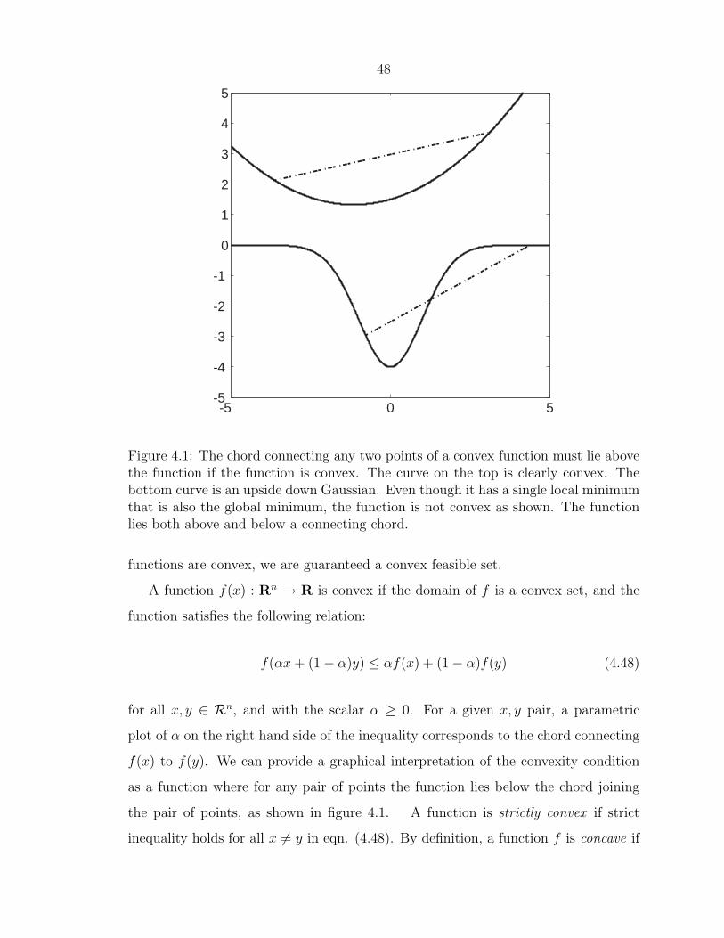
Figure 4.1: The chord connecting any two points of a convex function must lie abovethe function if the function is convex. The curve on the top is clearly convex. Thebottom curve is an upside down Gaussian. Even though it has a single local minimumthat is also the global minimum, the function is not convex as shown. The functionlies both above and below a connecting chord.

functions are convex, we are guaranteed a convex feasible set.

A function f(x) : Rn → R is convex if the domain of f is a convex set, and the

function satisfies the following relation:

f(αx + (1− α)y) ≤ αf(x) + (1− α)f(y) (4.48)

for all x, y ∈ Rn, and with the scalar α ≥ 0. For a given x, y pair, a parametric

plot of α on the right hand side of the inequality corresponds to the chord connecting

f(x) to f(y). We can provide a graphical interpretation of the convexity condition

as a function where for any pair of points the function lies below the chord joining

the pair of points, as shown in figure 4.1. A function is strictly convex if strict

inequality holds for all x 6= y in eqn. (4.48). By definition, a function f is concave if

49

(a) (b) (c)

Figure 4.2: Examples of convex and non-convex sets. The set of points in a polygon(a) and in an ellipse (b) are both convex. The star shape is not convex since theline connecting two points in the set passes through a region that is not in the set(highlighted in red).

-f is convex. For the rest of this chapter, we will only consider functions for which

the domain of f spans all of Rn, so the domain of f is always a convex set. Some

important examples of convex functions include

• Exponential eax is convex on R for any a ∈ R

• Logarithm log(x) is convex on 0 < x ∈ R

• Norms on Rn

• Linear, Affine, and Quadratic functions on Rn

• Non-negative weighted sums of convex functions f(x) = α1f1(x) + α2f2(x) for

f1, f2 convex functions and α1, α2 ≥ 0.

4.3.1 Convexity conditions

Suppose f is differentiable such that its gradient exists. The function f is convex if

and only if

f(y) ≥ f(x) +∇f(x)T (y − x) (4.49)

We recognize the right side of eqn. (4.49) as the multidimensional version of the lin-

ear Taylor series expansion of the function f about x. From this property of convex

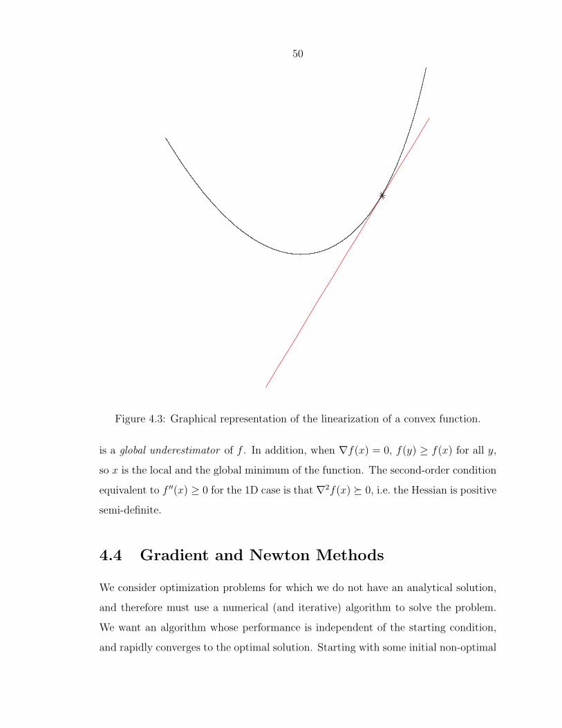
functions, we observe two consequences. First, linearization of the function underesti-

mates it everywhere (see figure 4.3). This means the first-order Taylor approximation

50

Figure 4.3: Graphical representation of the linearization of a convex function.

is a global underestimator of f . In addition, when ∇f(x) = 0, f(y) ≥ f(x) for all y,

so x is the local and the global minimum of the function. The second-order condition

equivalent to f ′′(x) ≥ 0 for the 1D case is that ∇2f(x) º 0, i.e. the Hessian is positive

semi-definite.

4.4 Gradient and Newton Methods

We consider optimization problems for which we do not have an analytical solution,

and therefore must use a numerical (and iterative) algorithm to solve the problem.

We want an algorithm whose performance is independent of the starting condition,

and rapidly converges to the optimal solution. Starting with some initial non-optimal

51

point x(0), each iterate (k) of the algorithm gives us an x(k) such that f0(x(k)) → f0(x

∗)

as k → ∞, where x∗ is the ‘true’ solution that optimizes our objective function. In

practice, the iterations terminate once some specified tolerance level is reached, i.e.

f(x(k)) − f(x∗) < ε. In general, this would be difficult to estimate, but because of

convexity it allows us to evaluate bounds on how far from optimal the final solution

is. At each iteration, the intermediate solution is updated via the following general

relation:

x(k+1) = x(k) + t(k)∆x(k) (4.50)

where ∆x(k) is an unnormalized vector in Rn known as a ‘step direction’ and t(k) > 0

is a scalar called the ‘step size’ for the kth iteration. Different algorithms will have

different methods for determining the step directions and step sizes. We consider only

descent methods here for which f(x(k+1)) ≤ f(x(k)), with equality only if f(x(k)) is

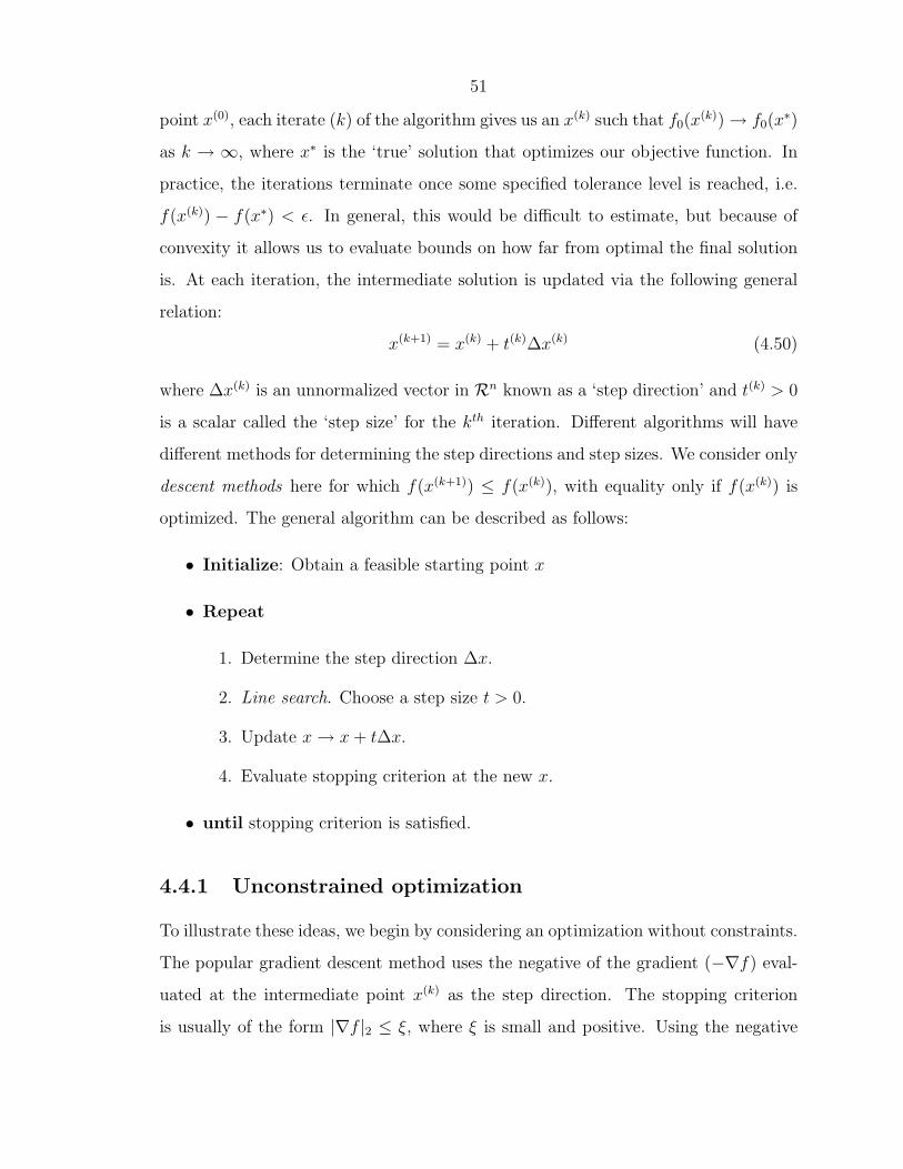
optimized. The general algorithm can be described as follows:

• Initialize: Obtain a feasible starting point x

• Repeat

1. Determine the step direction ∆x.

2. Line search. Choose a step size t > 0.

3. Update x → x + t∆x.

4. Evaluate stopping criterion at the new x.

• until stopping criterion is satisfied.

4.4.1 Unconstrained optimization

To illustrate these ideas, we begin by considering an optimization without constraints.

The popular gradient descent method uses the negative of the gradient (−∇f) eval-

uated at the intermediate point x(k) as the step direction. The stopping criterion

is usually of the form |∇f |2 ≤ ξ, where ξ is small and positive. Using the negative

52

gradient guarantees that our step direction is a descent direction, and for simple prob-

lems it is easy to implement in practice. Unfortunately, for ill-conditioned problems,

this method does not converge in practice. However, since the gradient is easy to

visualize, we include it here to help illustrate the second step of the algorithm, the

line search.

Backtracking Line Search

The line search is used to choose how far to step in the descent direction (once that

is determined). In principle, one can do an exact line search of the following form:

mint>0

f(x(k) + t∆x) (4.51)

which is a 1D minimization problem. However, in practice, inexact methods are

used because they are easier to implement without suffering a loss in performance.

Inexact methods aim to simply reduce the function by some sufficient amount, and

the backtracking line search is the one we will use. The algorithm depends on two

parameters α, β, with 0 < α < 0.5 and 0 < β < 1. It is called backtracking because

it first assumes a full step size of t = 1, and if the step does not lead to some

sufficient decrease in the objective function, then the step size is decreased by a

factor β so that t → βt (see figure 4.4). The sufficient decrease condition can be

written mathematically as:

f(x + t∆x) < f(x) + αt∇f(x)T ∆x. (4.52)

For small enough t, this condition must be true because we only consider descent

directions. The parameter α sets the amount of decrease in the objective function we

will accept as a percentage of the linear prediction (which, due to convexity, provides

a lower bound). Practical backtracking algorithms tend to have α between 0.01 and

0.3, and β between 0.1 and 0.8, with a small value of β corresponding to a coarser

grained search of the minimum.

53

1.5 1 0.5 0 0.5 1

4

3

2

1

0

1

Number of Backtracking Steps:5

t=0t=t0

t=1

t=β

t=β2 t=β3 t=β4

t=1

4

{α∆f

∆f

New x

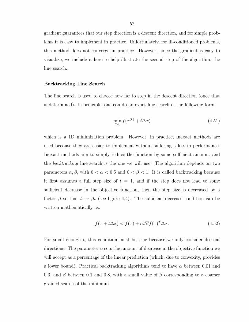
Figure 4.4: The linear approximation (red) to the objective function (black) expandedaround x = 0.64. The blue line shows the backtracking condition as accepting afraction α of the predicted decrease by linear extrapolation. After four backtrackingsteps, t = β4, and the value of the objective function has decreased enough.

As a simple example we choose the following 1D objective function:

f(x) = eγx + e−γx − 2, (4.53)

where γ is a parameter we will adjust to show the various behaviors of the gradient

descent method. The optimal value of x∗ is 0, and f(x∗) ≡ p∗ = 0. To illustrate the

idea of backtracking, we first show in figure 4.4 the objective function for γ = 1.25,

and choose as an initial point x0 = 0.64. The function is linearized at x0 in red, and

the blue line shows the backtracking condition for α = 0.2. A full step in the step

direction (t = 1) takes us to x = −1.5803, shown as a red star in the figure. As

illustrated, the region where the backtracking condition (eqn. (4.52)) is satisfied is

for t ∈ [0, t0]. Increasing α will decrease the size of the valid t region. The task for

the line search algorithm is to find a valid t. It backtracks from a starting value of

54

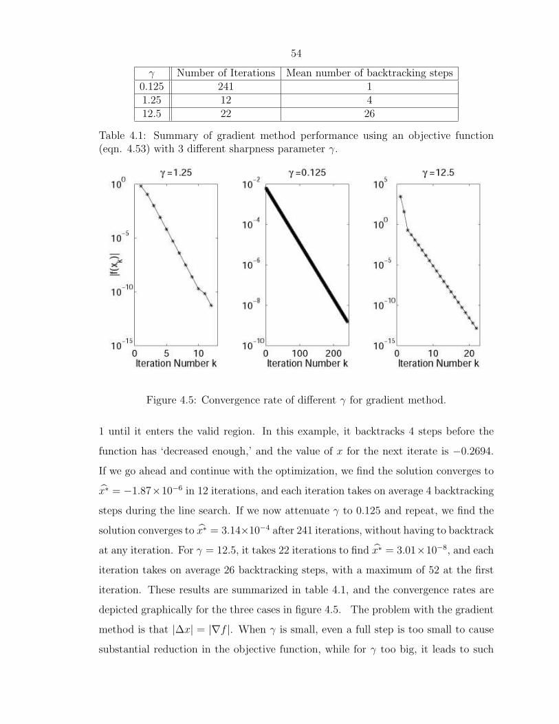
γ Number of Iterations Mean number of backtracking steps0.125 241 11.25 12 412.5 22 26

Table 4.1: Summary of gradient method performance using an objective function(eqn. 4.53) with 3 different sharpness parameter γ.

Figure 4.5: Convergence rate of different γ for gradient method.

1 until it enters the valid region. In this example, it backtracks 4 steps before the

function has ‘decreased enough,’ and the value of x for the next iterate is −0.2694.

If we go ahead and continue with the optimization, we find the solution converges to

x̂∗ = −1.87×10−6 in 12 iterations, and each iteration takes on average 4 backtracking

steps during the line search. If we now attenuate γ to 0.125 and repeat, we find the

solution converges to x̂∗ = 3.14×10−4 after 241 iterations, without having to backtrack

at any iteration. For γ = 12.5, it takes 22 iterations to find x̂∗ = 3.01×10−8, and each

iteration takes on average 26 backtracking steps, with a maximum of 52 at the first

iteration. These results are summarized in table 4.1, and the convergence rates are

depicted graphically for the three cases in figure 4.5. The problem with the gradient

method is that |∆x| = |∇f |. When γ is small, even a full step is too small to cause

substantial reduction in the objective function, while for γ too big, it leads to such

55

0 0.2 0.4 0.6 0.8

0

2

4

6

x 103

(b)

γ = 0.125

1 0 1

1

0

1

2

x 104 γ = 12.5

(a)

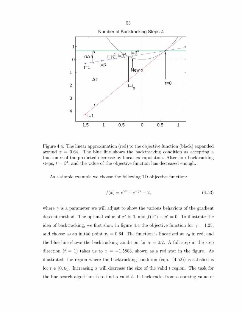
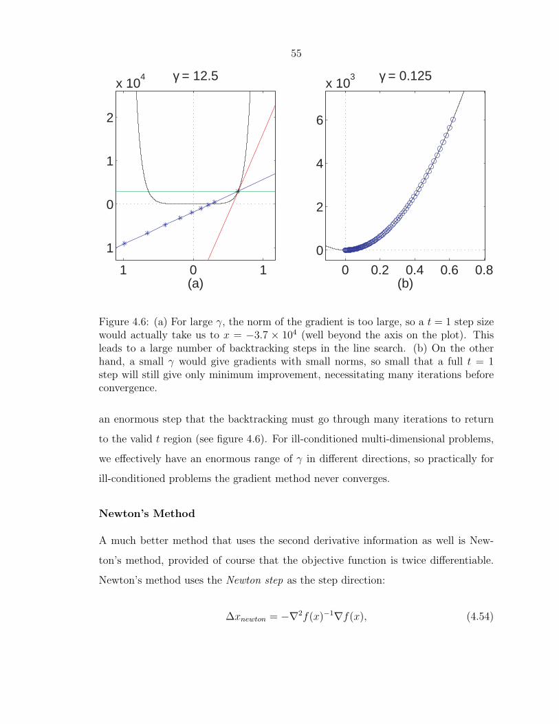
Figure 4.6: (a) For large γ, the norm of the gradient is too large, so a t = 1 step sizewould actually take us to x = −3.7 × 104 (well beyond the axis on the plot). Thisleads to a large number of backtracking steps in the line search. (b) On the otherhand, a small γ would give gradients with small norms, so small that a full t = 1step will still give only minimum improvement, necessitating many iterations beforeconvergence.

an enormous step that the backtracking must go through many iterations to return

to the valid t region (see figure 4.6). For ill-conditioned multi-dimensional problems,

we effectively have an enormous range of γ in different directions, so practically for

ill-conditioned problems the gradient method never converges.

Newton’s Method

A much better method that uses the second derivative information as well is New-

ton’s method, provided of course that the objective function is twice differentiable.

Newton’s method uses the Newton step as the step direction:

∆xnewton = −∇2f(x)−1∇f(x), (4.54)

56

0.5 0.6 0.7

1500

2000

2500

3000

3500

4000

4500

(a)

γ = 12.5

-0.5 0 0.5 1

0

0.5

1

1.5

(b)

γ = 1.25

-0.20

0.20.4

0.60.8

0

2

4

6

8

x 10

-3

(c)

γ = 0.125

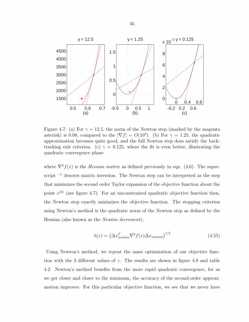
Figure 4.7: (a) For γ = 12.5, the norm of the Newton step (marked by the magentaasterisk) is 0.08, compared to the |∇f | = O(104). (b) For γ = 1.25, the quadraticapproximation becomes quite good, and the full Newton step does satisfy the back-tracking exit criterion. (c) γ = 0.125, where the fit is even better, illustrating thequadratic convergence phase.

where ∇2f(x) is the Hessian matrix as defined previously in eqn. (4.6). The super-

script −1 denotes matrix inversion. The Newton step can be interpreted as the step

that minimizes the second order Taylor expansion of the objective function about the

point x(k) (see figure 4.7). For an unconstrained quadratic objective function then,

the Newton step exactly minimizes the objective function. The stopping criterion

using Newton’s method is the quadratic norm of the Newton step as defined by the

Hessian (also known as the Newton decrement),

λ(x) =(∆xT

newton∇2f(x)∆xnewton

)1/2(4.55)

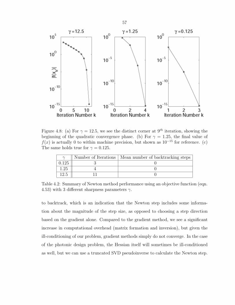
Using Newton’s method, we repeat the same optimization of our objective func-

tion with the 3 different values of γ. The results are shown in figure 4.8 and table

4.2. Newton’s method benefits from the more rapid quadratic convergence, for as

we get closer and closer to the minimum, the accuracy of the second-order approxi-

mation improves. For this particular objective function, we see that we never have

57

Figure 4.8: (a) For γ = 12.5, we see the distinct corner at 9th iteration, showing thebeginning of the quadratic convergence phase. (b) For γ = 1.25, the final value off(x) is actually 0 to within machine precision, but shown as 10−15 for reference. (c)The same holds true for γ = 0.125.

γ Number of Iterations Mean number of backtracking steps0.125 3 01.25 4 012.5 11 0

Table 4.2: Summary of Newton method performance using an objective function (eqn.4.53) with 3 different sharpness parameters γ.

to backtrack, which is an indication that the Newton step includes some informa-

tion about the magnitude of the step size, as opposed to choosing a step direction

based on the gradient alone. Compared to the gradient method, we see a significant

increase in computational overhead (matrix formation and inversion), but given the

ill-conditioning of our problem, gradient methods simply do not converge. In the case

of the photonic design problem, the Hessian itself will sometimes be ill-conditioned

as well, but we can use a truncated SVD pseudoinverse to calculate the Newton step.

58

4.4.2 Incorporating constraints: barrier method

Consider the following constrained optimization problem in 1D:

minimize f(x) = eγx + e−γx − 2 (4.56)

subject to x0 − x < 0 , x0 = 0.75. (4.57)

We have constructed the problem so that the solution to the constrained problem

lies at the boundary at x = 0.75. In order to incorporate inequality constraints, the

objective function is modified to include barrier functions that impose a prohibitively

costly penalty for violating the constraints. The barrier function that we will use is

the logarithmic barrier function, and we make use of the fact that the log diverges

near 0, meaning:

limx→0+

log x → −∞. (4.58)

Recall the set of inequality constraints from our optimization problem (eqn. (4.3))

require fi(x) ≤ 0 for all i. The logarithmic barrier function is defined to be

φ(x) ≡ −m∑

i=1

log(−fi(x)) (4.59)

Using the chain rule (eqn. (4.25) and (4.26)), we can write down the expression for

the gradient and Hessian for the log barrier function.

∇φ(x) =m∑

i=1

1

−fi(x)∇fi(x), (4.60)

∇2φ(x) =m∑

i=1

1

fi(x)2∇fi(x)∇fi(x)T +

m∑i=1

1

−fi(x)∇2fi(x) (4.61)

If we modify our objective function such that we instead minimize

f0(x) +

(1

δ

) m∑i=1

− log(−fi(x)) (4.62)

59

-0.8 -0.6 -0.4 -0.2 0 0.2-5

0

5

10

15

20

25

δ = 0.2δ = 1δ = 5Ideal

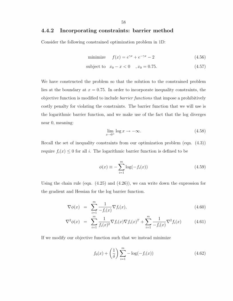
Figure 4.9: The log barrier function for various δ’s. The black dotted line is the idealstep barrier. Notice the largest of these (δ = 5) gives the closest approximation tothe ideal function.

we see that a violation of the inequality constraints will not minimize the objective

function. Therefore, the minimum of this new problem will automatically satisfy the

inequality constraints. The parameter δ controls how steep the barrier is. We plot

the barrier function for various δ’s in figure 4.9. As δ → ∞ , the barrier function

has no effect on the objective function for x in the feasible set, so this modified

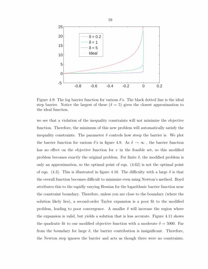
problem becomes exactly the original problem. For finite δ, the modified problem is

only an approximation, so the optimal point of eqn. (4.62) is not the optimal point

of eqn. (4.3). This is illustrated in figure 4.10. The difficulty with a large δ is that

the overall function becomes difficult to minimize even using Newton’s method. Boyd

attributes this to the rapidly varying Hessian for the logarithmic barrier function near

the constraint boundary. Therefore, unless you are close to the boundary (where the

solution likely lies), a second-order Taylor expansion is a poor fit to the modified

problem, leading to poor convergence. A smaller δ will increase the region where

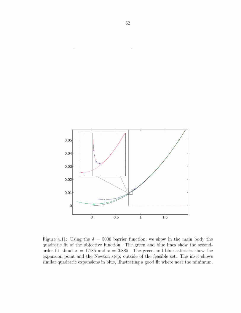
the expansion is valid, but yields a solution that is less accurate. Figure 4.11 shows

the quadratic fit to our modified objective function with a moderate δ = 5000. Far

from the boundary for large δ, the barrier contribution is insignificant. Therefore,

the Newton step ignores the barrier and acts as though there were no constraints.

60

1 2 30

0.05

0.1

0.15

0.2

(a)

δ = 10

1 2 30

0.05

0.1

0.15

0.2

(b)

δ = 100

1 2 30

0.05

0.1

0.15

0.2

δ = 5000

(c)

Figure 4.10: The modified objective function (red) for various δ’s. The constraint isthat x ≥ 0.75, and the optimal point is at the boundary (shown as a solid verticalblack line near the left edge of the box). The original objective function (black) hasγ = 0.125. The barrier function is the dotted red line. (a) δ = 10 The modifiedproblem is a poor approximation of the original. The optimal x∗ is around 2. (b)δ = 100 Slight improvement of the approximation, with x∗ ≈ 1. (c) δ = 5000 gives amuch better approximation.

However, this would take us out of the feasible set (main figure in figure 4.11). We have

the same problem here as we did with the gradient method then, as we potentially

may backtrack many iterations to return to the feasible set. Closer to the boundary,

the quadratic fit becomes quite good, as the barrier has an appreciable effect on the

modified function. The inset of figure 4.11 shows in blue the second-order fit and

Newton steps in that region. Of course, for large δ that means we are already very

close to the boundary, i.e. the solution of the optimization problem. A priori, we

would have no way of knowing where that fast converging region is.

The problem is overcome by a process called centering, where a succession of these

modified problems are solved with δ increasing with each centering step (δi+1 = µδi).

We solve the modified optimization problem using some small initial δ0 by Newton’s

method. The solution of a centering step is used as the starting point of the next

centering step. This ensures we are close to the region where Newton’s method

converges rapidly, as long as we don’t increase δ too quickly. This is reflected in the

61

parameter µ. If µ is too large, then we will have less centering steps, but each step

will require more iterations before it converges. If µ is too small, then we will require

many centering steps. Typical implementations take µ between 10 and 20.

For our implementation of the convex optimizer, we use for our line search routine

α = 0.125, and β = 0.9. Our stopping criterion is ε = 10−20, and µ = 20. Our

optimization problems uses 15 centering steps and within each centering step, the

solution will usually converge after less than 10 Newton steps.

4.5 Conclusion

In this chapter, we summarized some of the important tools needed for numerical op-

timization of multidimensional problems. Using a simple 1D example, we visualized

how the gradient descent algorithm and Newton’s method minimize a given objective

function. The caveat is that our intuition may or may not extend into N dimensions.

We can certainly imagine fitting the objective function with a hyper-paraboloid sur-

face, and minimizing that as the Newton step. In higher dimensions, it just shows

that the gradient has more directions to be incorrect about, so in practical problems

it is of little use.

We have now outlined all the tools we need to solve our photonic regularization

problem. We do not have equality constraints in our example, but those can be

satisfied by solving a set of KKT equations, as described in detail in Boyd. A final

note is that with these interior point methods, it is important to first find a feasible

point (i.e. satisfies all m inequality constraints and n equality constraints) as the

first iterate. Our constraints are simple enough that we can always construct one by

inspection (take a uniform slab of dielectric with an average index of refraction). In

general, there are algorithms loosely based on these techniques that serve as feasible

point finders.

62

0 0.5 1 1.5

0

0.01

0.02

0.03

0.04

0.05

Figure 4.11: Using the δ = 5000 barrier function, we show in the main body thequadratic fit of the objective function. The green and blue lines show the second-order fit about x = 1.785 and x = 0.885. The green and blue asterisks show theexpansion point and the Newton step, outside of the feasible set. The inset showssimilar quadratic expansions in blue, illustrating a good fit where near the minimum.