Embed Size (px)
Citation preview

Chapter 4: Coastal Wetlands
2013 Supplement to the 2006 IPCC Guidelines for National Greenhouse Gas Inventories: Wetlands 4.1
C H A PT ER 4
COASTAL WETLANDS

Chapter 4: Coastal Wetlands
4.2 2013 Supplement to the 2006 IPCC Guidelines for National Greenhouse Gas Inventories: Wetlands
Coordinating Lead Authors
Hilary Kennedy (UK), Daniel M. Alongi (Australia) and Ansarul Karim (Bangladesh)
Lead Authors
Guangcheng Chen (China), Gail L. Chmura (Canada), Stephen Crooks (USA), James G. Kairo (Kenya), Baowen
Liao (China) and Guanghui Lin (China)
Contributing Author
Tiffany G. Troxler (IPCC TFI TSU)
Review Editors
Nuria Marba Bordalba (Spain) and Georgi Karl Hiebaum (Bulgaria)

Chapter 4: Coastal Wetlands
2013 Supplement to the 2006 IPCC Guidelines for National Greenhouse Gas Inventories: Wetlands 4.3
Contents
4 Coastal Wetlands ....................................................................................................................................... 6
4.1 Introduction ...................................................................................................................................... 6
4.2 CO2 emissions and removals ........................................................................................................... 11
4.2.1 Forest management practices in mangroves .................................................................................. 11
4.2.1.1 Biomass ................................................................................................................................. 12
4.2.1.2 Dead organic matter ............................................................................................................... 16
4.2.1.3 Soil carbon ............................................................................................................................. 18
4.2.2 Extraction.................................................................................................................................... 18
4.2.2.1 Biomass ................................................................................................................................. 19
4.2.2.2 Dead organic matter ............................................................................................................... 23
4.2.2.3 Soil carbon ............................................................................................................................. 24
4.2.3 Rewetting, revegetation and creation of mangroves, tidal marshes and seagrass meadows ............. 26
4.2.3.1 Biomass ................................................................................................................................. 26
4.2.3.2 Dead organic matter ............................................................................................................... 27
4.2.3.3 Soil carbon ............................................................................................................................. 27
4.2.4 Drainage in mangroves and tidal marshes ................................................................................. 29
4.2.4.1 Biomass ................................................................................................................................. 30
4.2.4.2 Dead organic matter ............................................................................................................... 30
4.2.4.3 Soil carbon ............................................................................................................................. 30
4.3 Non-CO2 emissions ......................................................................................................................... 32
4.3.1 CH4 emissions from rewetted soils and created mangroves and tidal marshes................................ 32
4.3.1.1 Choice of method ................................................................................................................... 33
4.3.1.2 Choice of emission factors...................................................................................................... 33
4.3.1.3 Choice of activity data ............................................................................................................ 34
4.3.1.4 Uncertainty assessment .......................................................................................................... 34
4.3.2 N2O emissions during aquaculture use in mangroves, tidal marshes and seagrass meadows ........... 34
4.3.2.1 Choice of method ................................................................................................................... 35
4.3.2.2 Choice of emission factors...................................................................................................... 35
4.3.2.3 Choice of activity data ............................................................................................................ 36
4.3.2.4 Uncertainty assessment .......................................................................................................... 36
4.4 Completeness, time series consistency, and Quality Assurance and Quality Control (QA/QC) .......... 36
4.4.1 Completeness .............................................................................................................................. 36
4.4.2 Time series consistency ............................................................................................................... 36
4.4.3 Quality Assurance/Quality Control (QA/QC) ............................................................................... 36
Annex 4A.1 Salinity-based definitions ............................................................................................................ 37
Annex 4A.2 Estimation of above-ground mangrove biomass: higher tier methodology ..................................... 38
Annex 4A.3 Wood density of mangrove species .............................................................................................. 39

Chapter 4: Coastal Wetlands
4.4 2013 Supplement to the 2006 IPCC Guidelines for National Greenhouse Gas Inventories: Wetlands
Annex 4A.4 Percent refractory carbon ............................................................................................................. 40
Annex 4A.5 Derivation of N2O emission factor for aquaculture ....................................................................... 41
Appendix 4a.1 Future methodological development for estimating carbon export ............................................. 42
References ............................................................................................................................................... 43
Equations
Equation 4.1 Estimation of BCEF using BEF and wood densities ...................................................... 12
Equation 4.2 Tier 1 estimation of initial change in carbon stocks with extraction (all C pools) ........... 18
Equation 4.3 Initial change in carbon stocks with excavation (all C pools) ......................................... 18
Equation 4.4 Tier 1 estimation of initial change in biomass carbon stocks due to extraction activities . 20
Equation 4.5 Tier 1 estimation of initial change in dead organic matter carbon stocks due to extraction
activities ....................................................................................................................... 23
Equation 4.6 Tier 1 estimation of initial change in soil carbon stocks due to extraction activities ....... 24
Equation 4.7 CO2 emissions from rewetting, revegetation and creation of coastal wetlands ................ 28
Equation 4.8 CO2 emissions on drained organic and mineral soils ...................................................... 30
Equation 4.9 CH4 emissions from rewetted soils and created tidal marshes and mangroves................. 33
Equation 4.10 Direct N2O emissions from Aquaculture use ................................................................. 35
Figures
Figure 4.1 Decision tree to indicate relevant section for Tier 1 estimation of GHG emissions and
removals due to specific management activities in coastal wetlands. ................................ 9
Tables
Table 4.1 Specific management activities in coastal wetlands ......................................................... 6
Table 4.2 Carbon fraction of above-ground biomass (tonnes C (tonnes d.m.)-1) in mangroves ........ 13
Table 4.3 Above-ground biomass in mangroves (tonnes d.m. ha-1) ................................................ 14
Table 4.4 Above-ground biomass growth in mangroves (tonnes d.m. ha-1 yr-1) .............................. 14
Table 4.5 Ratio of below-ground biomass to above-ground biomass (R) in mangroves .................. 14
Table 4.6 Average density (D; tonnes m-3) of mangrove wood ...................................................... 15
Table 4.7 Tier 1 default values for litter and dead wood carbon stocks in mangroves ..................... 17
Table 4.8 Summary of Tier 1 estimation of initial changes in carbon pools for extraction activities ....................................................................................................................... 19
Table 4.9 Ratio of below-ground biomass to above-ground biomass (R) for tidal marshes ............. 21
Table 4.10 Ratio of below-ground biomass to above-ground biomass (R) for seagrass meadows ..... 21

Chapter 4: Coastal Wetlands
2013 Supplement to the 2006 IPCC Guidelines for National Greenhouse Gas Inventories: Wetlands 4.5
Table 4.11 Soil carbon stocks for mangroves, tidal marshes and seagrass meadows for extraction
activities ....................................................................................................................... 26
Table 4.12 Annual emission factors associated with rewetting (EFRE) on aggregated organic and mineral soils (tonnes C ha-1 yr-1) at initiation of vegetation reestablishment.................... 29
Table 4.13 Annual emission factors associated with drainage (EFDR) on aggregated organic and
mineral soils (tonnes C ha-1 yr-1) ................................................................................... 31
Table 4.14 Emission factors for CH4 (EFREWET) for Tier 1 estimation of rewetted land previously
vegetated by tidal marshes and mangroves .................................................................... 34
Table 4.15 Emission factor (EFF) for N2O emission from aquaculture use in mangroves, tidal marshes
and seagrass meadows .................................................................................................. 35
Boxes
Box 4.1 The following examples illustrate different management practices which may result in a
change of a land-use category depending on how countries define mangroves and other
coastal wetlands ............................................................................................................. 8

Chapter 4: Coastal Wetlands
4.6 2013 Supplement to the 2006 IPCC Guidelines for National Greenhouse Gas Inventories: Wetlands
4 COASTAL WETLANDS
4.1 INTRODUCTION
This chapter provides guidance on estimating and reporting anthropogenic greenhouse gas (GHG) emissions and
removals from managed coastal wetlands. Coastal wetlands hold large reservoirs of carbon (C) in biomass and especially soil [global stocks: mangroves, ~8 Pg C (Donato et al., 2011); tidal marshes, ~0.8 Pg C (midrange;
Pendleton et al., 2012); and seagrass meadows, 4.2 – 8.4 Pg C (Fourqurean et al., 2012)]. Soil carbon originates
largely in situ, from root biomass and litter, and can result in a significant pool in coastal wetlands, especially
when compared with terrestrial forests (Pidgeon, 2009).
Coastal wetlands generally consist of organic and mineral soils that are covered or saturated, for all or part of the
year, by tidal freshwater, brackish or saline water (Annex 4A.1) and are vegetated by vascular plants. The
boundary of coastal wetlands may extend to the landward extent of tidal inundation and may extend seaward to
the maximum depth of vascular plant vegetation. Countries need to develop a nationally appropriate definition of
coastal wetland taking into account national circumstances and capabilities. This chapter refers specifically to
tidal freshwater1 and salt marshes, seagrass meadows, and mangroves. For non-tidal inland mineral wetland soils,
refer to Chapter 5, this supplement.
1At the present time, insufficient data are available to provide generic default data for C pools in tidal freshwater swamps.
TABLE 4.1
SPECIFIC MANAGEMENT ACTIVITIES IN COASTAL WETLANDS
Activity Subactivity Vegetation types
affected
Activities relevant to CO2 emissions and removals
Forest
management
practices in mangroves
Planting, thinning, harvest, wood removal, fuelwood removal, charcoal production1
Mangrove2
Extraction
Excavation to enable port, harbour and marina construction and filling or dredging to facilitate raising the elevation of land
Mangrove, Tidal
marsh, Seagrass meadow4
Aquaculture (construction) Mangrove, Tidal
marsh
Salt production (construction) Mangrove, Tidal
marsh
Drainage Agriculture, forestry, mosquito control Mangrove, Tidal
marsh
Rewetting,
revegetation
and creation3
Conversion from drained to saturated soils by restoring hydrology and reestablishment of vegetation
Mangrove, Tidal marsh
Reestablishment of vegetation on undrained soils Seagrass meadow4
Activities relevant to non-CO2 emissions
Aquaculture
(use) N2O emissions from aquaculture use
Mangrove, Tidal
marsh, Seagrass meadow
Rewetted soils CH4 emissions from change to natural vegetation following modifications
to restore hydrology Mangrove, Tidal
marsh
1Including conversion to Forest Land or conversion from Forest Land to other land uses.
2 It is good practice to report mangroves in the appropriate national land-use category according to the national forest definition and to
consider when forest management practices may occur on mangroves classified under land-use categories other than Forest Land
(similar types of examples in inventory reporting include wood harvest from orchards or other perennial Cropland or harvest of trees from Wetlands). 3The term revegetation is used to refer to practices within the framework of UNFCCC reporting.
4Countries need to report on emissions from extraction and revegetation only if necessary data are available.

Chapter 4: Coastal Wetlands
2013 Supplement to the 2006 IPCC Guidelines for National Greenhouse Gas Inventories: Wetlands 4.7
It is good practice that inventory compilers determine a country-specific definition of coastal wetlands,
recognizing national circumstances. Having applied the country-specific definition, the specific management
activities (Table 4.1) need to be identified and emissions and removals reported using the methodologies provided in this chapter. When identifying the nature and location of these activities, inventory compilers need
only report GHG emissions or removals for activities where the anthropogenic contribution dominates over
natural emissions and removals. Management activities resulting in extraction of soils, such as construction of
aquaculture ponds, can result in large carbon dioxide (CO2) emissions in mangroves and tidal marshes. Nitrous
oxide (N2O) emissions can be significant from aquaculture activities. Rewetting increases methane (CH4)
emissions from drained freshwater tidal systems and increases carbon accumulation in mangrove biomass, dead
wood and soils.
Coastal wetlands can potentially occur in any land-use category defined in Chapter 3, Volume 4 of the 2006
IPCC Guidelines and the management activity may or may not result in a land-use change (see Box 4.1).
Regardless of whether a land-use change occurs, it is good practice to quantify and report significant emissions
and removals (Table 4.1) resulting from management activities on coastal wetlands in line with the country-specific definition. To cover all potential reporting options, new Wetland subcategories Other Wetlands
Remaining Other Wetlands and Land Converted to Other Wetlands are included. Coastal wetlands can also occur
on areas that are not part of the total land area of the country. Emissions and removals from these areas should be
reported separately under the relevant land-use category, however the associated land areas should be excluded
from the total area of the land-use category (refer to Chapter 7, this supplement). In this way, countries need not
be concerned with areas of coastal wetland, with small impacts on carbon stock changes and emissions of non-
CO2 gases, which are not included in the total land area.
Readers are referred to Volume 4 of the 2006 IPCC Guidelines for many of the basic equations to estimate GHG
emissions, and new guidance is provided in this chapter, as necessary. The decision tree (Figure 4.1) guides the
inventory compiler to the appropriate estimation methodology for each of the specific management activities
covered in this chapter.
COVERAGE OF THIS CHAPTER
This Chapter updates guidance contained in the 2006 IPCC Guidelines to:
provide default data for estimation of carbon stock changes in mangrove living biomass and dead wood
pools for coastal wetlands at Tier 1.
This Chapter gives new:
guidance for CO2 emissions and removals from organic and mineral soils for the management activities
of extraction (including construction of aquaculture and salt production ponds), drainage and rewetting,
revegetation and creation;
default data for estimation of anthropogenic CO2 emissions and removals for soils in mangrove, tidal marsh and seagrass meadows;
guidance for N2O emissions during aquaculture use;
guidance for CH4 emissions for rewetting, revegetation and creation of mangroves, tidal marshes and
seagrass meadows.
The Appendix to this Chapter provides the basis for future methodological development to address:
Anthropogenic emissions and removals associated with dissolved or particulate organic carbon (DOC,
POC) loss during drainage as affected by tidal exchange.
For constructed wetlands that occur in coastal zones that are modified to receive and treat wastewater, refer to
Chapter 6 (this supplement). Chapter 6 also covers semi-natural treatment wetlands, which are natural wetlands
where wastewater has been directed for treatment but the wetland is otherwise unmodified.
While countries will follow their own national definitions of coastal wetlands, some general features that may
help in consistent identification can be found throughout this guidance. It is good practice to maintain consistent
identification of lands for the purpose of reporting.

Chapter 4: Coastal Wetlands
4.8 2013 Supplement to the 2006 IPCC Guidelines for National Greenhouse Gas Inventories: Wetlands
BOX 4.1
THE FOLLOWING EXAMPLES ILLUSTRATE DIFFERENT MANAGEMENT PRACTICES WHICH MAY RESULT IN A
CHANGE OF A LAND-USE CATEGORY DEPENDING ON HOW COUNTRIES DEFINE MANGROVES AND OTHER
COASTAL WETLANDS
For Land remaining in a Land-use category (i.e. no change in land-use category), when:
Seagrass meadows or tidal marshes classified as Wetlands remain reported as Wetlands following
introduction of aquaculture activity.
Mangroves classified as Forest Land according to the national forest definition undergo selective
harvesting or biomass clearing remain reported as Forest Land unless they undergo a land-use
change.
Mangroves, which do not meet all thresholds of a country’s definition of forest, but are coastal
wetlands with trees are classified as Wetlands, and when subject to selective harvesting or biomass
clearing remain reported as Wetlands.
Conversely, management activities may result in a change in reporting category, for example,
when:
Seagrass meadows are initially classified as Wetlands, but are considered a Settlement following
introduction of aquaculture activity.
Tidal marshes are classified as Wetlands and are drained for agriculture and subsequently
classified as a Cropland or Grassland.
Mangroves are classified as Forest Land and undergo clearing, or drainage and converted to
another land-use category.
MANAGEMENT ACTIVITIES IN COASTAL WETLANDS
Coastal wetlands that have been modified by anthropogenic activities are often reduced in area. Globally about
35% of the area of mangroves has disappeared since 1980, with a current global areal rate of loss of between 0.7
and 3% yr-1 (Pendelton et al., 2012). The management activities that have led to the majority of mangrove loss
include forestry activities (26%) and aquaculture, comprising the construction (and extraction of soil) for shrimp
ponds (38%) and fish farms (14%) (Vaiela et al., 2009). Other management activities may lead to the removal of
mangrove biomass without necessarily resulting in mangrove clearance i.e. harvesting for fuelwood, charcoal
and construction. The current global areal rate of loss of tidal marsh is estimated to be between 1 and 2% yr-1
(Pendelton et al., 2012). Draining for agriculture, diking to isolate marsh from tides, filling (after extraction)
with sediment, and the extraction of soil during the construction of ponds for salt production are common management activities affecting tidal marshes. Seagrass meadows are experiencing a global areal rate of loss
currently of between 0.4 and 2.5% yr-1 (Pendelton et al., 2012). Globally, the main reasons for seagrass loss are
management activities such as dredging, leading to the excavation of soil to raise the elevation of land in low
lying areas and contribute to new land areas for settlement and aquaculture.
Revegetation efforts with mangroves, tidal marsh plants and seagrass, have been made worldwide to compensate
or mitigate for coastal wetland loss resulting from management activities (e.g. Bosire et al., 2008; Orth et al.,
2011). Recovery of vegetation that characterised the coastal zone generally requires reestablishment of the pre-
existing environmental setting, such as rewetting (restored hydrology), to maintain saturated soils and facilitate
plant growth. Management activities do not always affect all vegetation types (i.e. mangroves, tidal marsh plants
and seagrasses) or occur in all countries and not all coastal wetlands will be managed. To identify areas affected
refer to respective sections on Activity Data and throughout this supplement.

Chapter 4: Coastal Wetlands
2013 Supplement to the 2006 IPCC Guidelines for National Greenhouse Gas Inventories: Wetlands 4.9
Figure 4.1 Decision tree to indicate relevant section for Tier 1 estimation of GHG
emissions and removals due to specific management activities in coastal
wetlands2.
2 For extraction activities, CO2 emissions and removals are estimated for the initial change in carbon stocks that occur during
the year the extraction activities take place. Once the activity/activities is/are completed, these lands are continually tracked but CO2 emissions and removals are reported as zero at Tier 1. Forest management practices in mangroves, drainage and
rewetting are reported based on the area of land where it occurs, lands are tracked and CO2 emissions and removals subsequently are reported in the annual inventory.
Is biomass, DOM and soil
being extracted from this coastal
wetland?
No
Extraction (including
excavation, construction of
aquaculture and salt
production ponds)
Go to section 4.2.2 for CO2
Yes
Is the management activity
aquaculture and is it in use?
No
Is this an area being
managed to create or reestablish
seagrass meadows?
Aquaculture use
Go to section 4.3.2 for N2O
No
Yes
Does this coastal wetland
retain saturated soils and are mangrove forests
managed for wood harvesting or other
practices?
Forest management
practices in mangroves
Go to section 4.2.1. for CO2
Yes
Was this
a drained coastal wetland
and is now being rewetted or managed
to create or reestablish its
natural vegetation?
No
No
Has this coastal wetland
been drained?
Rewetting, revegetation &
creation
Go to section 4.2.3 for CO2
OR
Rewetted soils
Go to section 4.3.1 for CH4
Rewetting, revegetation &
creation
Go to section 4.2.3 for CO2
Drainage
Go to section 4.2.4 for CO2
Yes
Yes
Start
No guidance in this chapter
Yes
No

Chapter 4: Coastal Wetlands
4.10 2013 Supplement to the 2006 IPCC Guidelines for National Greenhouse Gas Inventories: Wetlands
The following sections provide some general information on the specified management activities in coastal
wetlands that result in large anthropogenic emissions and removals.
Forest management practices in mangroves
Removal of wood occurs throughout the tropics where mangrove forests are harvested for fuelwood, charcoal,
and construction (Ellison and Farnsworth, 1996; Walters et al., 2008). The wood removal can range from extensive forest clearing to more moderate, selective harvesting of individual trees, or to minimally invasive
activities such as bark removal. Natural disturbances are another form of biomass carbon stock loss. There may
also be conversion to forest land where mangrove replanting can take place on rewetted, or already saturated,
soils.
Extraction
Extraction collectively refers to:
(A) Excavation of saturated soils leading to unsaturated (drained) soils and removal of biomass and dead organic
matter. Activities that lead to the excavation of soil often lead to loss of coastal wetlands. The excavated or
dredged soil is also commonly used to help develop coastal infrastructure where there is a need to raise the elevation of land in low lying areas and/or contribute to new land areas for settlement.
(B) Excavation during the “construction” phase of aquaculture and salt production ponds in mangroves and tidal
marshes followed by the “use” of these facilities.
Aquaculture and salt production are common activities in the coastal zone and similarly require excavation of
soil and removal of biomass and dead organic matter for construction. There is a range of aquaculture practices,
but the most important are fish farming and production from shrimp ponds (World Bank, 2006). Salt production,
from the evaporation of seawater, is also a widespread activity with sites along tropical and subtropical coasts
worldwide, some of which have been producing salt for centuries (Oren, 2009; Thiery and Puente, 2002). In both
activities, ponds are constructed in mangroves and tidal marshes by clearing vegetation, levelling the soil and
subsequently excavating the surface soils to build berms where water is held. Depending on the type of
aquaculture (intensive, extensive etc.) and the species stocked in the ponds (shrimp, fish) the soils can be
excavated to make ponds of 0.5 m to 2.5 m depth (Cruz, 1997; Kungvankij et al., 1986; Wang, 1990; Robertson and Phillips, 1995). In a similar manner the depth of salt production ponds can vary between depths of about 0.5
to 2.5 m (e.g. Ortiz-Milan, 2006; Madkour and Gaballah, 2012).
Construction is only the first phase in aquaculture and salt production. The second phase, termed “use” is when
fish ponds, cages or pens are stocked and fish production occurs. In seagrass meadows, aquaculture is
maintained by housing fish in floating cages or pens that are anchored to the sediment (Alongi et al., 2009) and
these settings are considered during the use phase. N2O is emitted from aquaculture systems primarily as a by-
product of the conversion of ammonia (contained in fish urea) to nitrate through nitrification and nitrate to N2
gas through denitrification. The N2O emissions are related to the fish production (Hu et al., 2012). When use of
the aquaculture systems has been stopped, often due to disease or declining water clarity (Stevenson et al., 1999),
the systems transition to a final phase i.e. “discontinued”. All three phases (construction, use and discontinued)
of aquaculture and salt production are considered together with the other extraction activities, because the activity data are linked. However, only construction is addressed at Tier 1 for CO2, with higher tiers addressing
use and discontinued phases. For non-CO2, only the use phase is considered at Tier 1.
Rewett ing, revegetat ion and creation
Rewetting is a pre-requisite for vegetation reestablishment and/or creation of conditions conducive to purposeful
planting of vegetation that is characteristic of coastal wetlands. This activity is also used to describe the
management activities designed to reestablish vegetation on undrained soils in seagrass meadows. Once the
natural vegetation is established, soil carbon accumulation is initiated at rates commensurate to those found in
natural settings (Craft et al., 2002, 2003; Osland et al., 2012).
Rewetting in mangroves and tidal marshes occurs where hydrologic modifications reverse drainage or remove
impoundments or other obstructions to hydrologic flow (e.g. levee breach). Also included in this activity are
mangroves and tidal marshes that have been created, typically by raising soil elevation or removing the upper
layer of upland soil or dredge spoil, and grading the site until the appropriate tidal elevation is reached to
facilitate reestablishment of the original vegetation. Revegetation can occur by natural recolonisation, direct
seeding and purposeful planting. Alternatively, created wetlands with mangroves can be found where high
riverine sediment loads lead to rapid sediment accumulation, so that previously sub-aqueous soils can be elevated above tidal influence. This naturally created land can be reseeded or purposefully vegetated.

Chapter 4: Coastal Wetlands
2013 Supplement to the 2006 IPCC Guidelines for National Greenhouse Gas Inventories: Wetlands 4.11
The rewetting of tidal marshes and mangroves through reconnection of hydrology may lead to CH4 emissions
(Harris, 2010), particularly at low salinities, with an inverse relationship between CH4 emissions and salinity
(Purvaja and Ramesh, 2001; Poffenbarger et al., 2011).
In coastal wetlands where seagrass loss has occurred due to anthropogenic activities, soils remain saturated.
Initiatives to allow revegeation can include natural or purposeful dispersal of seed or planting of seagrass
modules (Orth et al., 2011). These same techniques can also be used to create (rather than re-establish) seagrass
meadows (Jones et al., 2012).
Drainage
Mangroves and tidal marshes have been diked and drained to create pastures, croplands and settlements since
before the 11th century (Gedan et al., 2009). The practice continues today on many coastlines. On some diked
coasts, groundwater of reclaimed former wetlands is pumped out to maintain the water table at the required level
below a dry soil surface, while on other coasts drainage is achieved through a system of ditches and tidal gates.
Due to the substantial carbon reservoirs of coastal wetlands, drainage can lead to large CO2 emissions.
4.2 CO2 EMISSIONS AND REMOVALS
This section provides the methodology to estimate CO2 emissions and removals from human activities in coastal
wetlands comprising forest management practices in mangroves, extraction, drainage and rewetting. The
methodological guidance provided here is consistent with methods for biomass and dead organic matter in
Volume 4 of the 2006 IPCC Guidelines and are in large part based on that methodological guidance: (1) for
forest management practices in mangroves, methods for biomass and dead organic matter are in large part based
on Chapter 4 of Volume 4; (2) for extraction activities, the methodological guidance is generally consistent with guidance for peat extraction Chapter 7 of Volume 4; and (3) for rewetting and drainage activities, updated
methodological guidance found in other chapters of this supplement is consistent with the methodologies
presented here. Activities covered by this chapter are described in Table 4.1. Separate guidance is provided on
estimation of changes in carbon stock from the five carbon pools.
Depending on circumstances, practices and definitions, specific coastal wetland management activities may or
may not involve a change in land-use category. The guidance in this chapter needs to be applied regardless of the
reporting categories. In particular, no recommendation is provided in relation to transition periods between land-
use categories; countries can apply the existing transition period of appropriate land-use categories.
Consistent with the 2006 IPCC Guidelines, the Tier 1 default approach assumes that the change in biomass and
dead organic matter carbon stocks are zero on all lands except on Forest Land or on Cropland, Grassland and
Wetlands with perennial woody biomass. On Forest Land and on Cropland, Grassland, or Wetlands with woody
biomass, the woody biomass and woody dead organic matter pools are potentially significant and need to be estimated in a manner consistent with the guidance provided in Chapters 2 (generic methods), 4 (Forest Land), 5
(Cropland), 6 (Grassland) and 7 (Wetlands) in Volume 4 of the 2006 IPCC Guidelines. Guidance provided here
refers to Equations 2.7, 2.8 and the subsequent equations in Chapter 2 of the 2006 IPCC Guidelines which split
the carbon stock changes in the biomass pool or ΔCB into the various possible gains and losses.
If specific management activities in coastal wetlands (Table 4.1) are accompanied by a change in land use that
involves Forest Land or Cropland, Grassland or Wetlands with perennial woody biomass, changes in carbon
stocks in biomass, dead wood and litter pools are equal to the difference in carbon stocks in the old and current
land-use categories (see Section 2.3.1.2, Chapter 2, Volume 4 of the 2006 IPCC Guidelines). These changes in
carbon stock occur only in the year of the conversion (extraction activities), or are uniformly distributed over the
length of the transition period (e.g. planting, harvesting). In soils the change in carbon stocks for extraction
activities occurs in the year of conversion, while for drainage, emissions persist as long as the soil remains drained or as long as organic matter remains, following the methodological guidance in this chapter.
4.2.1 Forest management practices in mangroves
This section deals with CO2 emissions and removals associated with forest management practices in mangroves.
It is good practice to follow a country’s national definition of forest, but also to apply the appropriate guidance
when mangrove wetlands have trees, but that do not necessarily satisfy all thresholds of the national definition of
forest. Depending on how the land is classified, forest management practices in mangroves may or may not lead
to a change in land-use category (examples provided in Box 4.1). For estimation methodologies refer to the
generic guidance provided in Chapter 2 of Volume 4 and more specific guidance in the relevant chapters of the
2006 IPCC Guidelines for reporting CO2 emissions and removals for above-ground biomass, below-ground biomass and dead organic matter (litter and dead wood).

Chapter 4: Coastal Wetlands
4.12 2013 Supplement to the 2006 IPCC Guidelines for National Greenhouse Gas Inventories: Wetlands
4.2.1.1 BIOMASS
Biomass can be stored in mangroves that contain perennial woody vegetation. The default methodology for
estimating carbon stock changes in woody biomass is provided in Section 2.2.1, Chapter 2, Volume 4 of the
2006 IPCC Guidelines. The change in biomass is only estimated for perennial woody vegetation of mangroves.
Changes in mangrove biomass may be estimated from either: 1) annual rates of biomass gain and loss (Equation 2.7, Chapter 2) or 2) changes in carbon stocks at two points in time (Equation 2.8, Chapter 2). The first approach
(Gain-Loss method) can be used for Tier 1 estimation (with refinements at higher tiers) whereas the second
approach can be used for Tier 2 or 3 estimations. It is good practice for countries to strive to improve inventory
and reporting approaches by advancing to the highest possible tier given national circumstances. For coastal
wetlands with non-woody vegetation (i.e. seagrass meadows and many tidal marshes), increase in biomass stocks
in a single year is assumed equal to biomass losses from mortality in that same year leading to no net change.
CHOICE OF METHOD
Tier 1
If the land (1) satisfies a country’s definition of forest or (2) is a mangrove wetland with trees, that nonetheless
do not meet the national definition of forest, and is managed for forest activities where no land-use change has
occurred, guidance is provided in “Section 2.3.1.1 Land Remaining in a Land-Use Category” and in the specific
guidance in Volume 4, of the IPCC 2006 Guidelines. Guidance is applied using the default data provided in this chapter (Table 4.2 – 4.6) and specific guidance below. Examples may include Forest Land to Forest Land,
Wetlands to Wetlands or Other Wetlands to Other Wetlands.
If the land (1) satisfies a country’s definition of forest or (2) is a mangrove wetland with trees, and is managed
for forest activities where land-use change has occurred or trees have been cleared, guidance is provided in
“Section 2.3.1.2 Land Converted to a Another Land-Use Category” and in the specific guidance in the relevant
chapters of Volume 4 of the 2006 IPCC Guidelines. Guidance is applied using the default data provided in this
chapter (Table 4.2 – 4.6) and specific guidance below.
When either the biomass stock or its change in a category (or sub-category) is significant or a key category, it is
good practice to select a higher tier for estimation. The choice of Tier 2 or 3 methods depends on the types and
accuracy of data and models available, level of spatial disaggregation of activity data and national circumstances.
If using activity data collected via Approach 1 (see Chapter 3 of Volume 4 in the 2006 IPCC Guidelines), and it
is not possible to use supplementary data to identify land converted from and to the respective land category, the inventory compiler needs to estimate carbon stocks in biomass following Section 2.3.1.1 and specific relevant
guidance as indicated above.
Because a biomass conversion and expansion factor (BCEF) is not available for mangroves, when above-ground
biomass is estimated from merchantable growing stock, for conversion of net annual increment, or for
conversion of woody and fuelwood removal volume to above-ground biomass removal, BCEF is derived from
wood density (Table 4.6) and a default value of BEF (Table 3A.1.10- Annex 3A.10 of the Good Practice
Guidance for Land Use, Land-use Change, and Forestry). This formulation follows Equation 4.1 and is
described in Box 4.2 of Chapter 4, Volume 4 of the 2006 IPCC Guidelines.
EQUATION 4.1
ESTIMATION OF BCEF USING BEF AND WOOD DENSITIES
BCEF = BEF • D
(Section 2.3.1.1, Chapter 2 of the 2006 IPCC Guidelines)
Where:
BCEF = biomass conversion and expansion factor for conversion of growing stock, net annual increment or
wood removals into above-ground biomass, above-ground biomass growth or biomass removals; tonnes
d.m. m-3
BEF = biomass expansion factor to expand the dry weight of the merchantable volume of growing stock,
net annual increment or wood removals to account for non-merchantable components; dimensionless
D = wood density; tonnes d.m. m-3
Tier 2
As in Tier 1, the Gain-Loss method can be applied using country-specific data. In addition, the Stock-Difference
method can also be applied using country-specific emission factors. If using the Stock-Difference method,
country-specific BEF or BCEF data or species specific wood density values (provided in Annex 4A.3) could be
applied. For Tier 2, countries may also modify the assumption that immediately following conversion to another

Chapter 4: Coastal Wetlands
2013 Supplement to the 2006 IPCC Guidelines for National Greenhouse Gas Inventories: Wetlands 4.13
land-use category, or after mangrove trees are cleared, biomass is zero. Refer to the relevant sections in Volume
4 of the 2006 IPCC Guidelines for further guidance on Tier 2 methodologies for forest management practices in
mangroves.
Tier 3
Tier 3 approach for biomass carbon stock change estimation allows for a variety of methods including process-
based models that simulate the dynamics of biomass carbon stock changes. Country-defined methodology can be based on estimates of above-ground biomass through use of allometric equations (Annex 4A.2) or include
detailed inventories based on permanent sample plots. Tier 3 could also involve substantial national data on
disaggregation by vegetation type, ecological zone and salinity. Tier 3 approaches can use growth curves
stratified by species, ecological zones, site productivity and management intensity. If developing alternative
methods, these need to be clearly documented. Refer to the relevant sections in Chapter 4, Volume 4 of the 2006
IPCC Guidelines for further guidance on Tier 3 methodologies for forest management practices in mangroves.
Spaceborne optical and radar data can be used for mapping changes in the extent of mangroves and transitions to
and from other land covers. Such techniques currently cannot routinely provide estimates of a sufficient level of
accuracy, although this may become more feasible in the future (refer to this section, “Choice of Activity Data”).
CHOICE OF EMISSION/REMOVAL FACTORS
Tier 1
For countries using the Gain-Loss method as a Tier 1 approach, the estimation of the annual carbon gains in
living biomass requires the following: carbon fraction of above-ground biomass, average above-ground biomass, mean annual above-ground biomass growth, ratio of below-ground biomass to above-ground biomass and
average wood density. The default values for these parameters are provided in Tables 4.2-4.6, respectively. It is
good practice to apply annual growth rates that lead neither to over- nor underestimates. Losses due to wood
removals, fuelwood removals and disturbances are also needed (refer to Choice of Activity Data for Tier 1 and
uncertainty analysis in this section).
Tier 2
National data could include country specific values of any parameter used in the Tier 1 method or values that
permit biomass carbon stock changes using the Stock-Difference method. Refer also to the relevant sections of
Volume 4 of the 2006 IPCC Guidelines for further guidance.
Tier 3
Tier 3 methods may employ the use of data that are of higher order spatial disaggregation and that depend on
variation in salinity or further disaggregation of regional differences within a country. Forest growth rates of
specific age ranges could be applied. Refer also to the relevant sections of Volume 4 of the 2006 IPCC
Guidelines for further guidance.
TABLE 4.2 CARBON FRACTION OF ABOVE-GROUND BIOMASS (TONNES C (TONNES D.M.)
-1) IN MANGROVES
1
Component %C 95% CI3 Range
Leaves + wood2 45.1 (n = 47) 42.9, 47.1 42.2-50.2
1This Table provides supplementary values to those presented in Table 4.3, Chapter 4, Volume 4 of the 2006 IPCC Guidelines.
2Sources: Spain and Holt, 1980; Gong and Ong, 1990; Twilley et al., 1992; Bouillon et al., 2007; Saenger, 2002; Alongi et al., 2003, 2004;
Kristensen et al., 2008 395% CI of the geometric mean
Chapter 4: Coastal Wetlands
4.14 2013 Supplement to the 2006 IPCC Guidelines for National Greenhouse Gas Inventories: Wetlands
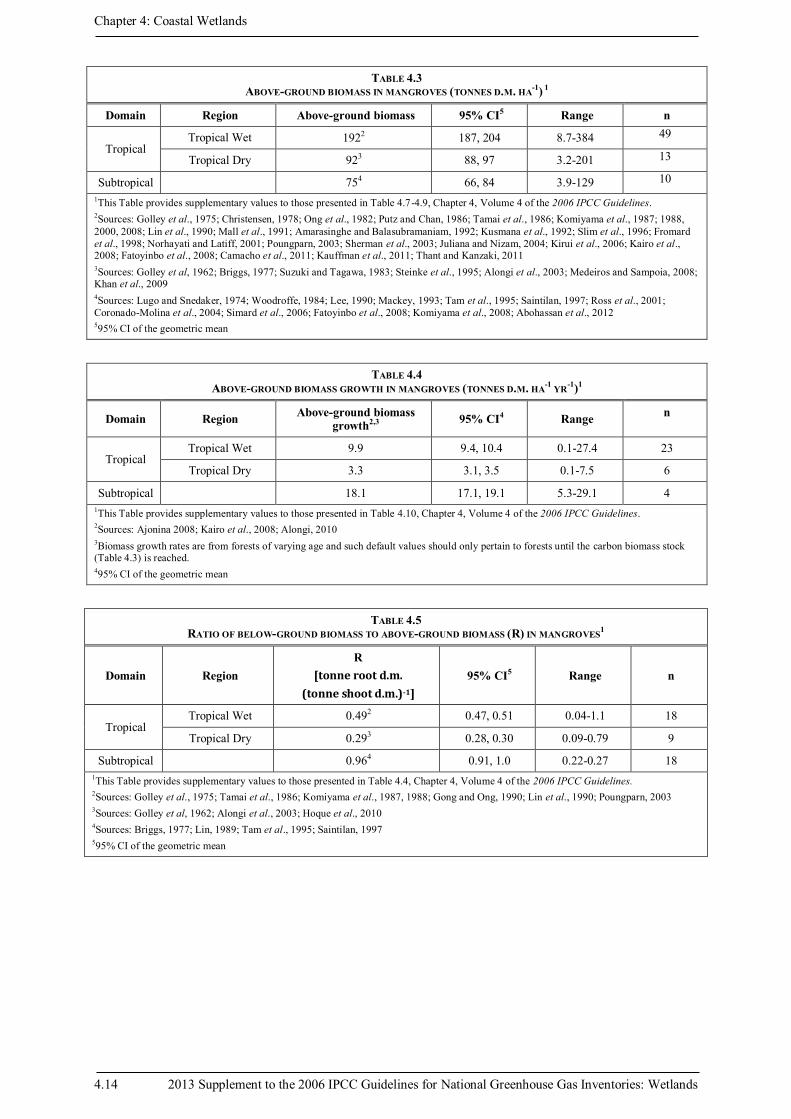
TABLE 4.3 ABOVE-GROUND BIOMASS IN MANGROVES (TONNES D.M. HA
-1)
1
Domain Region Above-ground biomass 95% CI5 Range n
Tropical Tropical Wet 1922 187, 204 8.7-384 49
Tropical Dry 923 88, 97 3.2-201 13
Subtropical 754 66, 84 3.9-129 10
1This Table provides supplementary values to those presented in Table 4.7-4.9, Chapter 4, Volume 4 of the 2006 IPCC Guidelines.
2Sources: Golley et al., 1975; Christensen, 1978; Ong et al., 1982; Putz and Chan, 1986; Tamai et al., 1986; Komiyama et al., 1987; 1988,
2000, 2008; Lin et al., 1990; Mall et al., 1991; Amarasinghe and Balasubramaniam, 1992; Kusmana et al., 1992; Slim et al., 1996; Fromard
et al., 1998; Norhayati and Latiff, 2001; Poungparn, 2003; Sherman et al., 2003; Juliana and Nizam, 2004; Kirui et al., 2006; Kairo et al., 2008; Fatoyinbo et al., 2008; Camacho et al., 2011; Kauffman et al., 2011; Thant and Kanzaki, 2011
3Sources: Golley et al, 1962; Briggs, 1977; Suzuki and Tagawa, 1983; Steinke et al., 1995; Alongi et al., 2003; Medeiros and Sampoia, 2008;
Khan et al., 2009 4Sources: Lugo and Snedaker, 1974; Woodroffe, 1984; Lee, 1990; Mackey, 1993; Tam et al., 1995; Saintilan, 1997; Ross et al., 2001;
Coronado-Molina et al., 2004; Simard et al., 2006; Fatoyinbo et al., 2008; Komiyama et al., 2008; Abohassan et al., 2012 595% CI of the geometric mean
TABLE 4.4
ABOVE-GROUND BIOMASS GROWTH IN MANGROVES (TONNES D.M. HA-1
YR-1
)1
Domain Region Above-ground biomass
growth2,3
95% CI
4 Range
n
Tropical Tropical Wet 9.9 9.4, 10.4 0.1-27.4 23
Tropical Dry 3.3 3.1, 3.5 0.1-7.5 6
Subtropical 18.1 17.1, 19.1 5.3-29.1 4
1This Table provides supplementary values to those presented in Table 4.10, Chapter 4, Volume 4 of the 2006 IPCC Guidelines.
2Sources: Ajonina 2008; Kairo et al., 2008; Alongi, 2010
3Biomass growth rates are from forests of varying age and such default values should only pertain to forests until the carbon biomass stock
(Table 4.3) is reached. 495% CI of the geometric mean
TABLE 4.5 RATIO OF BELOW-GROUND BIOMASS TO ABOVE-GROUND BIOMASS (R) IN MANGROVES
1
Domain Region
R
[tonne root d.m.
(tonne shoot d.m.)-1]
95% CI5 Range n
Tropical Tropical Wet 0.492 0.47, 0.51 0.04-1.1 18
Tropical Dry 0.293 0.28, 0.30 0.09-0.79 9
Subtropical 0.964 0.91, 1.0 0.22-0.27 18
1This Table provides supplementary values to those presented in Table 4.4, Chapter 4, Volume 4 of the 2006 IPCC Guidelines.
2Sources: Golley et al., 1975; Tamai et al., 1986; Komiyama et al., 1987, 1988; Gong and Ong, 1990; Lin et al., 1990; Poungparn, 2003
3Sources: Golley et al, 1962; Alongi et al., 2003; Hoque et al., 2010
4Sources: Briggs, 1977; Lin, 1989; Tam et al., 1995; Saintilan, 1997
595% CI of the geometric mean

Chapter 4: Coastal Wetlands
2013 Supplement to the 2006 IPCC Guidelines for National Greenhouse Gas Inventories: Wetlands 4.15
TABLE 4.6 AVERAGE DENSITY (D; TONNES M
-3) OF MANGROVE WOOD
1
D 95% CI
2 Range n
Wood 0.71 0.64, 0.74 0.41-0.87 85
1Sources: Global Wood Density Database http://datadryad.org/resource/doi:10.5061/dryad.234/1?show=full; Saenger, 2002; Komiyama et
al., 2005; Donato et al., 2012 295% CI of the geometric mean
CHOICE OF ACTIVITY DATA
All tiers require information on areas of forest management practices in mangroves. Information on mangrove
forest types as well as soil types can be obtained from national wetland and soil type maps (if available) or the
International Soil Reference and Information Centre (www.isric.org). Mangrove distributions for most countries can be obtained from the RAMSAR web site (www.ramsar.org). When information is gathered from multiple
sources, it is good practice to conduct crosschecks to ensure complete and consistent representation and avoid
omissions and double-counting.
Tier 1
For Tier 1, these data can be obtained from one of the following sources3:
FAOSTAT http://faostat.fao.org/
Global Mangrove Database & Information System: http://www.glomis.com/
The UNESCO Mangrove Programme: http://www.unesco.org/csi/intro/mangrove.htm
Mangrove and the Ramsar Convention: http://www.ramsar.org/types_mangroves.htm
USGS Global Mangrove Project http://lca.usgs.gov/lca/globalmangrove/index.php
Mangrove.org: http://mangrove.org/
Mangrove Action Project: http://www.mangroveactionproject.org/
FAO Mangrove Management: http://www.fao.org/forestry/mangrove/en/
USGS National Wetlands Research Center: http://www.nwrc.usgs.gov/index.html
World Atlas of Mangrove: http://data.unep-wcmc.org/datasets/22
World Distribution of Coral Reefs and Mangroves: http://www.unep-wcmc.org
For Tier 1 estimation, FAO data sources can be used to estimate wood removal and fuelwood removal. Further
sources of activity data can be found in the relevant sections of Volume 4 of the 2006 IPCC Guidelines.
Additional resources can be found in IPCC (2010).
Global mangrove cover has been mapped by the United States Geological Service (USGS) for three epochs
“1975” (1973-1983), “1990” (1989 – 1993), and “2000” (1997 -2000) and is available for download at
http://edcintl.cr.usgs.gov/ip/mangrove/download.php. Global distribution of Mangroves (V3.0, 1997) has been
compiled by UNEP World Conservation Monitoring Centre (UNEP-WCMC) in collaboration with the
International Society for Mangrove Ecosystems (ISME).
The Kyoto & Carbon Initiative of the Japan Aerospace Exploration Agency (JAXA) Global Mangrove Watch
project has used Synthetic Aperture Radar mosaics to create maps of global mangrove extent for the years 1995 and 2007-2010 (JAXA 2010a) and maps of annual changes in mangrove areas between the years 1995-2007,
2007-2008, 2008-2009 and 2009-2010. (http://www.eorc.jaxa.jp/ALOS/en/kyoto/mangrovewatch.htm).
Resources providing recent trends in coastal wetland area can help countries understand circumstances of those
trends and what management activities contribute to them (FAO, 2007; Green and Short, 2003;
http://archive.org/stream/worldatlasofseag03gree#page/n5/mode/2up; JAXA, 2010b; Sifleet et al., 2011;
http://nicholasinstitute.duke.edu/publications?topics=34; Fatoyinbo and Simard, 2013).
Sources providing international data can be verified, validated and updated data with national sources.
3If these links do not work, either paste into your browser or do a web search for the resources or institution.
Chapter 4: Coastal Wetlands
4.16 2013 Supplement to the 2006 IPCC Guidelines for National Greenhouse Gas Inventories: Wetlands
Tiers 2 and 3
At Tiers 2 and 3, country-specific activity data is applied, and at Tier 3, at the resolution required for Tier 3
methods. At higher tiers, these data may be obtained from local, state or regional government department
websites as many countries and regional government authorities report this information. Countries also have
their own remote sensing systems which can be used for land change mapping (Nasciemto et al., 2013) Wood
density values (Annex 4A.3) of specific species need to be applied at Tiers 2 and 3. Areas of extensive harvesting of mangroves may be assessed with aerial imagery. When the ALOS-2 satellite is operational,
generation of annual radar mosaics and mangrove extent and change maps is planned
(http://www.eorc.jaxa.jp/ALOS/en/kyoto/mangrovewatch.htm).
UNCERTAINTY ASSESSMENT
The major sources of uncertainty for all wetland types, especially mangroves, are dominant species-specific
differences in carbon content and differences due to forest age, species composition, intertidal location, soil
fertility and community structure. The confidence intervals presented in Tables 4.2 - 4.6, range from about 24%
to 200%. To reduce uncertainty, countries are encouraged to develop country- or region-specific BEFs and
BCEF values. In case country- or region-specific values are unavailable, it is good practice to check the sources of default parameters and their correspondence with species present, as well as with the conditions in country.
The causes of variation of annual increment of mangrove growth include climate, site growth conditions, and
soil fertility. Artificially regenerated and managed stands are less variable than natural forests. One of the ways
to improve accuracy of estimates of these wetlands includes the application of country-specific or regional
estimates of growth stratified by the dominant species present. If the default values of growth increments are
used, the uncertainty of the estimates need to be clearly indicated and documented.
For mangroves, data on commercial fellings are relatively accurate, although they may be incomplete or biased
due to illegal fellings and under-reported due to tax regulations. Traditional wood that is gathered and used
directly, without being sold, is not likely to be included in any statistics. Countries must carefully consider these
issues. The amount of wood removed from forests after storms and pest outbreaks varies both in time and
volume. No default data can be provided on these types of losses. The uncertainties associated with these losses
can be estimated from the amount of damaged wood directly withdrawn from the forest or using data on damaged wood subsequently used for commercial and other purposes. If fuelwood gathering is treated separately
from fellings, the relevant uncertainties might be high, due to the level of uncertainty associated with traditional
gathering.
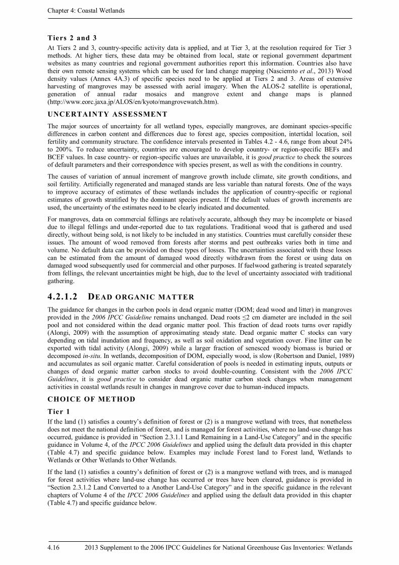
4.2.1.2 DEAD ORGANIC MATTER
The guidance for changes in the carbon pools in dead organic matter (DOM; dead wood and litter) in mangroves
provided in the 2006 IPCC Guideline remains unchanged. Dead roots ≤2 cm diameter are included in the soil
pool and not considered within the dead organic matter pool. This fraction of dead roots turns over rapidly (Alongi, 2009) with the assumption of approximating steady state. Dead organic matter C stocks can vary
depending on tidal inundation and frequency, as well as soil oxidation and vegetation cover. Fine litter can be
exported with tidal activity (Alongi, 2009) while a larger fraction of senesced woody biomass is buried or
decomposed in-situ. In wetlands, decomposition of DOM, especially wood, is slow (Robertson and Daniel, 1989)
and accumulates as soil organic matter. Careful consideration of pools is needed in estimating inputs, outputs or
changes of dead organic matter carbon stocks to avoid double-counting. Consistent with the 2006 IPCC
Guidelines, it is good practice to consider dead organic matter carbon stock changes when management
activities in coastal wetlands result in changes in mangrove cover due to human-induced impacts.
CHOICE OF METHOD
Tier 1
If the land (1) satisfies a country’s definition of forest or (2) is a mangrove wetland with trees, that nonetheless
does not meet the national definition of forest, and is managed for forest activities, where no land-use change has
occurred, guidance is provided in “Section 2.3.1.1 Land Remaining in a Land-Use Category” and in the specific guidance in Volume 4, of the IPCC 2006 Guidelines and applied using the default data provided in this chapter
(Table 4.7) and specific guidance below. Examples may include Forest land to Forest land, Wetlands to
Wetlands or Other Wetlands to Other Wetlands.
If the land (1) satisfies a country’s definition of forest or (2) is a mangrove wetland with trees, and is managed
for forest activities where land-use change has occurred or trees have been cleared, guidance is provided in
“Section 2.3.1.2 Land Converted to a Another Land-Use Category” and in the specific guidance in the relevant
chapters of Volume 4 of the IPCC 2006 Guidelines and applied using the default data provided in this chapter
(Table 4.7) and specific guidance below.

Chapter 4: Coastal Wetlands
2013 Supplement to the 2006 IPCC Guidelines for National Greenhouse Gas Inventories: Wetlands 4.17
Tier 2
Estimation methodologies for Tier 2 can follow Tier 1 methods, but apply country-specific data. The Stock-
Difference method (Chapter 4, Volume 4 of the 2006 IPCC Guidelines) could also be applied if countries have
sample plot data from forest inventories for two points in time. Literature data or carbon databases may provide
more feasible and cost-effective data to apply this method.
Tier 3
Loss estimates of dead wood and litter due to tidal movement (export) can also be considered (Appendix 4a.1).
Tier 3 methods may further employ stratification by ecological zone or disturbance regime to reduce
uncertainties. It is good practice to sum changes in both dead wood and litter to report changes in total dead
organic matter. Additional Tier 3 guidance is provided in Chapter 4, Volume 4 of the 2006 IPCC Guidelines.
CHOICE OF EMISSION/REMOVAL FACTORS
Tier 1
Default values are provided in Table 4.7 of this supplement for use in Tier 1 assessment of emissions and
removals.
Tier 2
Tier 2 methods using country-specific data can be used if such country-specific data can be acquired at
reasonable cost.
Tier 3
Tier 3 emission factors include model output and validation and disaggregated data sources. Field measurements
can be developed and used to inform and validate model output at Tier 3. For mangroves, Tier 3 methodologies
can employ empirical relationships to provide estimates of canopy litter fall and census of downed wood lying
on the forest floor.
TABLE 4.7
TIER 1 DEFAULT VALUES FOR LITTER AND DEAD WOOD CARBON STOCKS IN MANGROVES
Domain Ecosystem
type Litter C stocks of mature stands
(tonnes C ha-1
) with 95% CI1
Dead wood C stocks of mature stands (tonnes C ha
-1) with 95% CI
1
Tropical/Subtropical mangroves 0.7 (0-1.3) 10.7 (6.5-14.8)
Litter: Utrera-Lopez and Moreno-Casasola, 2008; Liao et al., 1990; Chen et al., 2008; Richards et al., 2011; Ramose-Silva et al., 2007;
Twilley et al., 1986
Dead Wood: Kauffman et al., 2011; Donato et al., 2012; Allen et al., 2000; Steinke et al., 1995; Robertson et al., 1989; Tam et al., 1995; Krauss et al., 2005 195% CI of the geometric mean
CHOICE OF ACTIVITY DATA
Tier 1
Carbon stock changes in dead organic matter are generally not reported at Tier 1 when management activities in
coastal wetlands do not result in changes in mangrove cover due to human-induced impacts (following guidance
in Section 4.2.2.3 of Chapter 4, Volume 4 of the 2006 IPCC Guidelines), and thus no activity data are required.
If a land-use change has occurred resulting from an increase in woody biomass stock, it is good practice to
report the change in dead organic matter carbon stock. For a Tier 1 method, the annual rate of conversion to
Forest Land or other land-use categories with woody mangrove biomass is required, following Section 4.3.2.3 of
Chapter 4, Volume 4 of the 2006 IPCC Guidelines. Activity data should be consistent with those used for
estimating changes in carbon stock.
Tier 2 and Tier 3
Inventories using higher tiers will require more comprehensive information on the establishment of new forests,
using climate, for example, as a disaggregating factor and at higher spatial and temporal resolution. Additional
resources can be found in IPCC (2010).
UNCERTAINTY ASSESSMENT
The uncertainty assessment given in section 4.2.2.5 in Chapter 4, Volume 4 of the 2006 IPCC Guidelines
identifies sources of uncertainty in estimates of carbon stock changes in the dead organic matter pool of

Chapter 4: Coastal Wetlands
4.18 2013 Supplement to the 2006 IPCC Guidelines for National Greenhouse Gas Inventories: Wetlands
mangroves. Other sources of uncertainty include output of dead organic matter due to decomposition or tidal
export.
4.2.1.3 SOIL CARBON
The Tier 1 default assumption is that soil CO2 emissions and removals are zero (EF=0) for forest management
practices in mangroves. This assumption can be modified at higher tiers. At higher tiers, it is recommended to
consider CO2 emissions from soils due to forest clearing in carbon stock estimations (Alongi et al., 1998). It
should also be considered that at Tier 1, rewetting (section 4.2.3) and drainage activities (section 4.2.4) can occur
as a result of forest management practices. In this case, follow the guidance for estimating CO2 emissions and
removals from soil carbon stock changes (Sections 4.2.3.3 and 4.2.4.3, respectively).
4.2.2 Extraction
Extraction refers collectively to the following activities: (A) excavation (associated with dredging used to
provide soil for raising the elevation of land, or excavation to enable port, harbour and marina construction and
filling), (B) construction of aquaculture ponds and (C) construction of salt production ponds (where soil is
excavated to build berms where water is held in ponds). Each of these extraction activities is associated with the
removal of biomass, dead organic matter and soil, which results in significant emissions when their removal is
from saturated (water-logged) to unsaturated (aerobic) conditions (World Bank, 2006). The Tier 1 methodology
assumes that the biomass, dead organic matter and soil are all removed and disposed of under aerobic conditions
where all carbon in these pools is emitted as CO2 during the year of the extraction with no subsequent changes.
Tier 1 guidance is given here for reporting the intial changes in carbon (Table 4.1). Regardless of whether the extraction activities result in a change in land-use category, CO2 emissions and removals associated with
extraction are the same, following Equation 4.2 below. This approach follows the methodology applied for peat
extraction in Chapter 7, Volume 4 of the 2006 IPCC Guidelines.
EQUATION 4.2
TIER 1 ESTIMATION OF INITIAL CHANGE IN CARBON STOCKS WITH EXTRACTION
(ALL C POOLS)
ΔCEXT = ΔCexcav + ΔCaq-constr + ΔCsp-constr
Where:
ΔCEXT = Changes in carbon stocks from all extraction activities; tonnes C
ΔCexcav = Initial change in biomass, dead organic matter and soil carbon stocks from extraction due to
excavation; tonnes C
ΔCaq-constr = Initial change in biomass, dead organic matter and soil carbon stocks from extraction during
construction of aquaculture ponds; tonnes C
ΔCsp-constr = Initial change in biomass, dead organic matter and soil carbon stocks from extraction during construction of salt production ponds; tonnes C
Equation 4.2 is applied to the total area of coastal wetland where extraction activities take place. The terms
ΔCexcav, ΔCaq-constr, and ΔCsp-constr are estimated as ΔCCONVERSION (Equations 4.4 - 4.6) for intial change in carbon
stocks of each of the C pools for each of the respective activities comprising extraction. Equation 4.3 is applied
for each of the extraction activities (and A-C as described above) to estimate the intial change in stocks of each
of the C pools.
EQUATION 4.3
INITIAL CHANGE IN CARBON STOCKS WITH EXCAVATION (ALL C POOLS)
ΔCexcav = ΔCexcav-AB + ΔCexcav-BB + ΔCexcav-DOM + ΔCexcav-SO
Where:
ΔCexcav = Initial change in biomass, dead organic matter and soil carbon stocks with excavation; tonnes C
ΔCexcav-AB = Initial change in above-ground biomass carbon stock changes with excavation; tonnes C
ΔCexcav-BB = Initial change in below-ground biomass carbon stock changes with excavation; tonnes C
ΔCexcav-DOM = Initial change in dead organic matter carbon stock changes with excavation; tonnes C

Chapter 4: Coastal Wetlands
2013 Supplement to the 2006 IPCC Guidelines for National Greenhouse Gas Inventories: Wetlands 4.19
ΔCexcav-SO = Initial change in soil carbon stock changes with excavation as annual CO2 emissions and
removals; tonnes C
At Tier 1,
ΔCexcav-AB + ΔCexcav-BB= ΔCB-CONVERSION (Equation 4.4, Section 4.2.2.1)
ΔCexcav-DOM = ΔCDOM-CONVERSION (Equation 4.5, Section 4.2.2.2)
ΔCexcav-SO = ΔCSO-CONVERSION (Equation 4.6, Section 4.2.2.3)
Equation 4.3 provides the formulation to estimate the initial change in carbon stock in each C pool for the
specific extraction activity, excavation. To estimate the initial changes in intial carbon stock change for these
pools for construction of aquaculture and salt production ponds, replace ΔCexcav with ΔCaq-constr and ΔCsp-constr in
Equation 4.3, respectively.
The Tier 1 methodology assumes that the biomass, dead organic matter and soil are all removed and disposed of
under aerobic conditions where all carbon in these pools is emitted as CO2 during the year of extraction
(consistent with the assumption applied for peat extraction in Section 7.2.1.1, Chapter 7, Volume 4 of the 2006
IPCC Guidelines) and that no subsequent changes occur.
Table 4.8 summarises the Tier level guidance provided for extraction activities, which deals with excavation in
general and excavation during the construction phase of aquaculture and salt production, in particular. Estimates
are not made at Tier 1 for CO2 emissions and removals while (1) fish ponds are stocked and salt production is
occuring (use phase of aquaculture and salt production) or (2) when the activity has ceased (discontinued phase),
although they are considered together with other extraction activities because the activity data are linked.
TABLE 4.8 SUMMARY OF TIER 1 ESTIMATION OF INITIAL CHANGES IN CARBON POOLS FOR EXTRACTION ACTIVITIES
C pools
Mangrove
biomass,
dead wood and litter
1
Soils
Mangrove and Tidal Marsh Seagrass Meadow
Organic Mineral Mineral2
Extr
act
ion
act
ivit
ies Excavation Tier 1 Tier 1 Tier 1 Tier 1
Aquaculture
and Salt
Production
Construction Tier 1 Tier 1 Tier 1 NA3
Use No guidance4 Discontinued No guidance4
1Removal of biomass resulting from extraction activities is estimated at Tier 1 level in mangroves only.
2Tier 1 assumption is that all seagrass soils are mineral.
3Extraction activity of aquaculture pond construction, is not applicable for seagrass meadows.
4No suitable Tier 1 methodologies are available for C pools during these phases/activities.
4.2.2.1 BIOMASS
This section addresses estimation of changes in living (above and below-ground) biomass pools associated with
extraction activities comprising excavation, and construction of aquaculture and salt production ponds in coastal
wetlands. For extraction in coastal wetlands with tidal marshes and seagrass meadows, changes in biomass
carbon stocks are reported at only Tier 2 or higher estimations. It is good practice to report the conversion of above-ground and below-ground biomass that occurs with extraction of mangroves.
CHOICE OF METHOD
Following Box 4.1 extraction may or may not result in a change in land-use category, however the same
methodologies apply for mangrove wetlands with forest regardless of how the land is classified.
Tier 1
Changes in carbon stock of living biomass during extraction are associated with clearing and removal of
vegetation. The area applied is that of a certain year in which the conversion occurs. Regardless of the land-use
category, the loss in biomass associated with extraction activities is estimated as ∆Cconversion following the

Chapter 4: Coastal Wetlands
4.20 2013 Supplement to the 2006 IPCC Guidelines for National Greenhouse Gas Inventories: Wetlands
methodology for peat extraction (Chapter 7, Volume 4 of the 2006 IPCC Guidelines), modified here as Equation
4.4.
EQUATION 4.4
TIER 1 ESTIMATION OF INITIAL CHANGE IN BIOMASS CARBON STOCKS DUE TO EXTRACTION
ACTIVITIES
ΔCB-CONVERSION = ∑v,c{BAFTER • (1+R) − BBEFORE * (1+R)} • CF • ACONVERTEDv,c
Where:
ΔCB-CONVERSION = Changes in biomass carbon stock from conversion due to extraction activities; tonnes C
BAFTER = Carbon stock in above-ground biomass per unit of area immediately after the conversion by
vegetation type (v) and climate (c); tonnes d.m. ha-1; default value = 0
BBEFORE = Carbon stock in above-ground biomass per unit of area immediately before the conversion;
tonnes d.m. ha-1
R = ratio of below-ground biomass to above-ground biomass by vegetation type (v) and climate (c); tonnes
d.m. below-ground biomass (tonnes d.m. above ground biomass)-1
CF = carbon fraction of dry matter; tonnes C (tonnes d.m.)-1
ACONVERTED = Area of conversion by vegetation type (v) and climate (c); ha
The Tier 1 methodology assumes that the biomass is removed and disposed of under aerobic conditions where all
carbon is emitted as CO2 during the year of the extraction and that no subsequent changes occur. At Tier 1,
initial change in carbon stocks of biomass {BAFTER • (1+R) − BBEFORE • (1+R)} is assumed to be zero for coastal
wetlands without perennial biomass or trees. For mangrove wetlands with perennial biomass or trees, the stock
after the conversion (BAFTER) at Tier 1 is taken to be zero.
Tier 2
At Tier 2, changes of carbon stock in living above-ground biomass of tidal marsh and seagrass meadow
vegetation can be estimated and reported for the specified activities employing the equation for ΔCB-CONVERSION,
using country-specific emission factors and default values for R given in Tables 4.9 and 4.10, in conjunction
with country-specific data on above-ground biomass. At Tier 2, the Gain-Loss or Stock-Difference methods can
be applied to estimate biomass carbon stock changes of mangrove in lands where extraction activities (aquaculture and salt production) are discontinued (i.e. regrowth). Tier 2 approaches could also include
evaluation of the assumption of instantaneous oxidation of the converted biomass pool.
Tier 3
In Tier 3, estimation could include methods to incorporate data on the fraction of biomass carbon stock that is retained under saturated conditions to improve estimation of proportion of carbon that is oxidized.
CHOICE OF EMISSION/REMOVAL FACTORS
Tier 1
Default data for Tier 1 method is provided for mangroves in Tables 4.2-4.6, Section 4.2.1, including above-
ground biomass carbon stock, carbon fraction and below-ground to above-ground ratio, for the different climate
domains and regions, where applicable.
Tier 2
Under Tier 2, countries apply country-specific data to estimate changes in carbon stock in above-ground biomass.
The conversion of above-ground and below-ground biomass that occurs with extraction activities in tidal marsh
and seagrass meadows may be estimated using Tables 4.9 and 4.10 for tidal marshes and seagrass meadows respectively. These data are to be used in conjunction with the carbon fraction of dry matter alongside country-
specific data on above-ground biomass carbon stock.
Tier 3
Field measurements can be developed and used to inform and validate model output at Tier 3. It is expected that
data improvements for excavation activities such as ground-truth estimates of overall area impacted, the depth at
which removal of biomass has occurred, or the fraction of biomass removal, could be used to develop and verify
models.

Chapter 4: Coastal Wetlands
2013 Supplement to the 2006 IPCC Guidelines for National Greenhouse Gas Inventories: Wetlands 4.21
TABLE 4.9 RATIO OF BELOW-GROUND BIOMASS TO ABOVE-GROUND BIOMASS (R) FOR TIDAL MARSHES
Domain
R
[tonne root d.m. (tonne shoot d.m.)
-1]
95% CI5 Range n
Mediterranean 3.631 3.56, 3.70 1.09-7.15 5
Subtropical 3.652 3.56, 3.74 2.23-9.41 5
Temperate
freshwater tidal 1.153 1.12, 1.18 0.36-3.85 7
Temperate 2.114 2.07, 2.15 0.33-10.15 17
1Sources: Scarton et al., 2002; Neves et al., 2007; Boyer et al., 2000
2Sources: Lichacz et al., 1984; da Cunha Lana et al., 1991
3Sources: Birch and Cooley, 1982; Whigham et al., 1978
4Sources: Kistritz et al., 1983; Hussey and Long, 1982; Smith et al., 1979; Dunn, 1981; Connor and Chmura, 2000; Gross et al.,
1991; Whigham et al., 1978; Elsey-Quirk et al., 2011; Adams et al., 2012 595% CI of the geometric mean
CHOICE OF ACTIVITY DATA
Extraction: Submissions of licenses for prospecting and exploitation and associated environmental impact
assessments (EIAs) can be used to obtain areas under extraction activities. Relevant regulation for extraction can
be found at international and national levels. International regulation is covered by the UN Convention on the
Law of the Sea (UNCLOS) 1982 (www.un/org/Depts/los/index.htm). Contracting Parties are under the
obligation to publish/communicate reports on monitoring and assessment of potential harmful effects of
extraction. The OSPAR Convention 1992 (www.ospar.org) provides guidance for programmes and measures for the control of the human activities in the North-East Atlantic region. The “Agreement on Sand and Gravel
Extraction” provides that authorisation for extraction of marine soils from any ecologically sensitive site should
be granted after consideration of an EIA. The Helsinki Convention 1992 (www.helcom.fi) covers the Baltic Sea
Area and requires EIAs to be carried out as part of the extraction process and that “monitoring data” and “results
of EIA’s………be made available for scientific evaluation”. The Barcelona Convention 1995
TABLE 4.10
RATIO OF BELOW-GROUND BIOMASS TO ABOVE-GROUND BIOMASS (R) FOR SEAGRASS MEADOWS
Domain
R
[tonne root d.m.
(tonne shoot d.m.)-1
]
95% CI4 Range n
Tropical 1.71 1.5, 1.9 0.05-25.62 396
Subtropical 2.42 2.3, 2.6 0.07-16.8 391
Temperate 1.33 1.1, 1.5 0.14-13.8 91
1Sources: Aioi and Pollard, 1993; Brouns, 1985; Brouns, 1987; Coles et al., 1993; Daby, 2003; Devereux et al., 2011; Fourqurean
et al., 2012; Halun et al., 2002; Holmer et al., 2001; Ismail, 1993; Lee, 1997; Lindeboom and Sandee, 1989; McKenzie, 1994;
Mellors et al., 2002; Moriarty et al., 1990; Nienhuis et al., 1989; Ogden and Ogden, 1982; Paynter et al., 2001; Poovachiranon
and Chansang, 1994; Povidisa et al., 2009; Rasheed, 1999; Udy et al., 1999; van Lent et al., 1991; van Tussenbroek, 1998; Vermaat et al., 1993; Vermaat et al., 1995; Williams, 1987 2Sources: Aioi, 1980; Aioi et al., 1981; Asmus et al., 2000; Bandeira, 2002; Boon, 1986; Brun et al., 2009; Collier et al., 2009; de
Boer, 2000; Devereux et al., 2011; Dixon and Leverone, 1995; Dos Santos et al., 2012; Dunton, 1996; Fourqurean et al., 2012;
Hackney, 2003; Herbert and Fourqurean, 2008; Herbert and Fourqurean, 2009; Holmer and Kendrick, 2012; Jensen and Bell,
2001; Kim et al., 2012; Kirkman and Reid, 1979; Kowalski et al., 2009; Larkum et al., 1984; Lee et al., 2005; Lee et al., 2005b;
Lipkin, 1979; Longstaff et al.,1999; Masini et al., 2001; McGlathery et al., 2012; McMahan, 1968; Meling-Lopez and Ibarra-
Obando, 1999; Mukai et al., 1979; Paling and McComb, 2000; Park et al., 2011; Powell, 1989; Preen, 1995; Schwarz et al., 2006;
Stevensen, 1988; Townsend and Fonseca, 1998; Udy and Dennison, 1997; van Houte-Howes et al., 2004; van Lent et al., 1991; van Tussenbroek, 1998; Walker, 1985; West and Larkum, 1979; Yarbro and Carlson, 2008 3Sources: Agostini et al., 2003; Cebrian et al., 2000; Fourqurean et al., 2012; Hebert et al., 2007; Holmer and Kendrick, 2012;
Larned, 2003; Lebreton et al., 2009; Lillebo et al., 2006; Marba and Duarte, 2001; McRoy, 1974; Olesen and Sand-Jensen, 1994; Rismondo et al., 1997; Sand-Jensen and Borum, 1983; Terrados et al., 2006 495% CI of the geometric mean

Chapter 4: Coastal Wetlands
4.22 2013 Supplement to the 2006 IPCC Guidelines for National Greenhouse Gas Inventories: Wetlands
(www.unepmap.org), covers the regulatory framework for the Mediterranean. The ICES Convention 1964
(www.ices.dk) provides data handling services to OSPAT and Helsinki Commissions. An overview of the
regulation of marine aggregate operations in some European Union Member States is reported in Radzevicius et al. (2010) and includes relevant EC Directives and national legislation/regulation. Other such sources of activity
data include, for example, statistics on sand and gravel extraction for the OSPAR martime area (e.g.
www.ospar.org/documents/dbase/publications/p0043) as well as information on sand and gravel activities and
related statistics for North Sea Continental Shelfs and UK waters (http://www.sandandgravel.com/).
If time series data back to 1990 are unavailable, it is suggested that surrogate data be used, derived from
statistical reports/databases containing information on temporal changes in proxy factors such as human
population density, port or marina development, port revenue, shipping tonnage, and commodity exports. Such
data can be obtained from the internet e.g. for the Asia-Pacific region from the UN ESCAP Commission
(http://www. unescap.org/stat/) and for the Baltic from
http://epp.eurostat.ec.europa.eu/portal/page/portal/statistics/themes. Data on shipping indices can be obtained
from http://www.worldshipping.org/about-the-industry/global trade/trade-statistics. Such data for most countries can also be obtained from http://datacatalog.worldbank.org.
Aquaculture and salt production: Annual data (1950 – present) providing statistics on aquaculture production
is collated by the FAO Fisheries and Aquaculture Department. Additional data on type aquaculture (e.g.
freshwater or brackish) and area under aquaculture production is summarised in country profiles enabling
stratification of aquaculture into those occurring in coastal wetlands
(http://www.fao.org/fishery/countryprofiles/search/en). As local regulations typically apply for developing new
aquaculture activites (i.e licensing, permitting), regulations also typically apply to report such activities to the
Ministry of Fisheries and Marine Affairs (or country equivalent). For example an aquaculture farm needs to get a
license (or permission) to operate. Depending on the country, it is given by the regional (e.g. in Spain it is the
autonomic, e.g. Balearic- government, who approves it) or local (e.g. at Bolinao, The Philipines) and maybe in
others the national government. For example, in Indonesia local government must be consulted on land-use
change including aquaculture pond construction and are obliged to report activities to the Ministry of Fisheries and Marine Affairs.
Similar project information for salt production activities can be obtained from the Salt Institute at
www.saltinstitute.org.
Literature sources can also provide national area change statistics from aerial photographs of ponds or structures
used for aquaculture and salt production.
A map of available tidal marsh distribution (with area data) is in production by the World Conservation and
Monitoring Center (WCMC; http://data.unep-wcmc.org/) currently holding layers for Europe, the United States,
Australia and China. It is the intent to expand mapping of tidal marsh to global coverage.
A map of global distribution of seagrasses (V2.0, 2005) is also available at the WCMC (http://data.unep-
wcmc.org/) and prepared in collaboration with Dr. Frederick T. Short. Other regional and national maps are also
available (e.g. http://www.ospar.org/documents/dbase/publications/p00426_zostera_beds). A tabulated list of web sites for existing seagrass monitoring programmes is given in Borum et al., (2000;
http://www.seagrasses.org/handbook/european_seagrasses_high.pdf).
These data sources, and those provided in Section 4.2.1.1, can be used in conjunction with activity data
described above to improve estimations of areas of mangroves, tidal marsh and seagrass meadow undergoing
extraction activities.
UNCERTAINTY ASSESSMENT
For uncertainty assessment for mangroves, see Section 4.2.1 (this chapter). The uncertainties involved in
extraction in mangroves also follow those outlined in Section 4.3.1.5 of Chapter 4, Volume 4 of the 2006 IPCC Guidelines. Variability in tidal marsh biomass will be due to differences in dominant species and competition
between species, as well as salinity of flood waters, frequency of tidal flooding and climate. For example, the
high biomass in mediterranean climates is due to the frequent dominance of perennial shrubs. For all vegetation
there can be considerable interannual variability in production of biomass and seasonal variability in standing
biomass that contributes to uncertainty in ratios of below-ground to above-ground biomass. Most empirical data
are available from temperate regions and North America and there are limited data available for tidal freshwater
and boreal and subtropical tidal marshes. The average ratio of below-ground to above-ground biomass for
seagrass is variable depending on the dominant species, and fertility of the soil. The data are mainly derived
from observations along the coasts of North America, Western Europe and Australia. Data were scarce from
South America and Africa.

Chapter 4: Coastal Wetlands
2013 Supplement to the 2006 IPCC Guidelines for National Greenhouse Gas Inventories: Wetlands 4.23
4.2.2.2 DEAD ORGANIC MATTER
Previously saturated dead organic matter (DOM), which is exposed to aerobic conditions, can contribute to large
sources of CO2 emissions from extraction activities. Consistent with the 2006 IPCC Guidelines for Forest Land,
in coastal wetlands, it is good practice to consider dead organic matter carbon stock changes when extraction
activities result in changes in mangrove cover due to these human-induced impacts.
CHOICE OF METHOD
Tier 1
During extraction activities, existing dead organic matter pools may be reduced to zero as vegetation is cleared
and removed while at the same time no new carbon enters the dead organic matter pool. At Tier 1, changes in
carbon stock in dead organic matter in tidal marshes and seagrass meadows are assumed to be zero. It is noted,
however, that extraction activities that result in vegetation or soil disturbance in tidal marsh with perennial
woody biomass may have significant impacts on CO2 emissions and removals. It is good practice for country-
specific methods to be developed to cover these cases, if feasible. Regardless of the land-use category, the loss in
dead organic matter associated with extraction activities is estimated as ∆Cconversion following the methodology
applied for peat extraction (Chapter 7, Volume 4 of the 2006 IPCC Guidelines), modified here as Equation 4.5:
EQUATION 4.5
TIER 1 ESTIMATION OF INITIAL CHANGE IN DEAD ORGANIC MATTER CARBON STOCKS DUE TO
EXTRACTION ACTIVITIES
ΔCDOM-CONVERSION = ∑v(DOMAFTER − DOMBEFORE)v • ACONVERTEDv
Where:
ΔCDOM-CONVERSION = Initial changes in dead organic matter carbon stock from conversion due to extraction
activities by vegetation type (v); tonnes C
DOMAFTER = Carbon stock in dead organic matter per unit of area immediately after the conversion by
vegetation type (v); tonnes d.m. ha-1; default value = 0
DOMBEFORE = Carbon stock in dead organic matter per unit of area immediately before the conversion by
vegetation type (v); tonnes d.m. ha-1
ACONVERTED = Area of conversion by vegetation type (v); ha
The Tier 1 methodology assumes that the dead organic matter is removed and disposed of under aerobic
conditions where all carbon is emitted as CO2 during the year of the extraction and that no subsequent changes
occur. The choice of method follows that in Section 4.2.2.
Tiers 2 and 3
The choice of method follows that in Section 4.2.2. For these management activities that impact dead organic
matter pools in tidal marshes with perennial or woody biomass, Tier 2 and higher estimation methods are
recommended.
CHOICE OF EMISSION/REMOVAL FACTORS
Tier 1
Default values of dead organic matter carbon stock (for dead wood and litter) for mangroves are provided in
Table 4.7 of this supplement for use in Tier 1 estimations. In tidal marsh and seagrass meadows the Tier 1
assumption is that carbon stocks in the dead organic matter pools resulting from extraction activities are zero.
Tier 2
At Tier 2, the assumption that all dead organic matter lost in the year of conversion is oxidized can be reassessed.
Tier 2 assumption of zero for dead organic matter pools in tidal marsh can also be assessed. It is good practice
for countries, in such cases, to use national estimates for dead organic matter carbon stocks for mangroves and
tidal marshes with perennial biomass, if such country-specific data can be acquired at reasonable cost.
Tier 3
Tier 3 emission factors include model output and validation and disaggregated data sources.

Chapter 4: Coastal Wetlands
4.24 2013 Supplement to the 2006 IPCC Guidelines for National Greenhouse Gas Inventories: Wetlands
CHOICE OF ACTIVITY DATA
Choice of activity data follows from guidance provided in Section 4.2.2.1. The area in which the extraction
activities occur will be the same area applied for each carbon pool, especially forest biomass.
UNCERTAINTY ASSESSMENT
The discussion on uncertainty outlined in Section 4.3.2.5 of Chapter 4, Volume 4 of the 2006 IPCC Guidelines is
also relevant for extraction of mangroves.
4.2.2.3 SOIL CARBON
Extraction activities that occur within coastal wetlands can influence organic and mineral stocks of carbon in
soils and both soil types are covered at Tier 1 (Table 4.11). During extraction activities, the stock of soil carbon
that is removed depends on the soil type (i.e. carbon stock is higher in organic soils). For Tier 1 estimation, in the
absence of soil map data or other resources to differentiate soil type, the following assumptions can be applied.
i. Assume that soils in which seagrass grow are mineral.
ii. Assume all soils, regardless of dominant vegetation in or at the mouth of estuaries or adjacent to any river
characterised by a large and/or mountainous catchment and high flow, are mineral. For all other
mangroves and tidal marshes the soils are organic. See Durr et al. (2011) for additional national level
guidance.
iii. If soils cannot be dissagregated into organic and mineral, use the aggregated default data given in Table 4.11.
CHOICE OF METHOD - ORGANIC AND MINERAL SOILS
Tier 1
Regardless of the land-use category, the loss in soil carbon associated with extraction activities is estimated as
∆Cconversion following the methodology applied for peat extraction (Chapter 7, Volume 4 of the 2006 IPCC
Guidelines), modified here as Equation 4.6.
EQUATION 4.6
TIER 1 ESTIMATION OF INITIAL CHANGE IN SOIL CARBON STOCKS
DUE TO EXTRACTION ACTIVITIES
ΔCSO-CONVERSION = ∑v,s(SOAFTER − SOBEFORE)v,s • ACONVERTEDv,s
Where,
ΔCSO-CONVERSION = Initial changes in soil carbon stock from conversion due to extraction activities by
vegetation type (v) and soil type (s); tonnes C
SOAFTER = Soil carbon stock per unit of area, immediately after the conversion, by vegetation type (v) and
soil type (s); tonnes C ha-1; default value = 0
SOBEFORE = Soil carbon stock per unit of area, immediately before the conversion, by vegetation type (v)
and soil type (s); tonnes C ha-1
ACONVERTED = Area of conversion by vegetation type (v) and soil type (s); ha
At Tier 1, soil extraction depth to 1 m approximates the mid-range of the extraction depth for construction of
aquaculture and salt production ponds (see extraction activities in section 4.1). Countries may modify the
assumption of 1 m extraction depth at higher tiers.
The Tier 1 methodology assumes that the soil is removed and disposed of under aerobic conditions where the carbon stock is emitted as CO2 (oxidised) during the year of the extraction. The carbon stock is taken as all soil
carbon except any refractory (unoxidisable) carbon. In mangrove soils, 4% of the carbon stock is refractory
(Annex 4A.4) and this is taken to be representative of the refractory carbon in tidal marshes and seagrass
meadows as well. Therefore, after the initial conversion of the soil pool in the year in which the activity occurs,
CO2 emissions are reported as zero. It is good practice to track these lands to consider management activities
that may occur on those lands in the future and for higher tier estimations. The choice of method follows that in
Section 4.2.2. For Tier 1, CO2 emissions are reported as the conversion in soil carbon where this activity occurs;
the type of vegetation and the available activity data to distinguish between organic and mineral soils determines
which data are applied from Table 4.11.

Chapter 4: Coastal Wetlands
2013 Supplement to the 2006 IPCC Guidelines for National Greenhouse Gas Inventories: Wetlands 4.25
Tier 2
At Tier 2, methodology can be applied to disaggregate by vegetation type and soil type. For the specific
extraction activity, countries may use national data to determine their particular extraction processes and the
volume of soil removed, if sufficient data are available. Because tidal marshes can occur in a range of climates,
disaggregating by climate may also be applied to improve estimates if those country-specific data are available.
Tier 2 may also refine the estimate for the soil carbon stock that is excavated to construct the aquaculture or salt production ponds by including country-specific information on the depth excavated during the construction
phase.
Tier 3
Tier 3 methods can employ models to estimate CO2 emissions based on the effect of temperature and salinity on soil oxidation both seasonally and with climate and vegetation type. At Tier 3, it is good practice for countries to
validate models with field measurements. Tier 3 methods may also include site-specific measurements of, for
example, carbon content, bulk density, clay content, salinity, redox potential, etc., to determine the underlying
processes of emissions.
CHOICE OF EMISSION FACTORS - ORGANIC AND MINERAL SOILS
Tier 1
Default Tier 1 soil carbon stocks (to 1 m depth) for mangrove, tidal marsh and seagrass meadows for the
calculation of CO2 emissions are given in Table 4.11. These values are to be used in conjunction with Equation
4.6 to estimate emissions. If soil type is not known, a generic default value for aggregated organic and mineral
soils can be applied (Table 4.11).
Tier 2
Tier 2 includes the use of country-specific emission factors that can be applied to disaggregate by soil type and
vegetation type to improve on Tier 1 estimates. Country-specific data may include excavation depth to improve
on the default estimation of soil extracted.
Tier 3
A Tier 3 approach could use models that take into account the time-dependent nature of the CO2 fluxes over a
range of timescales. For example, during the construction phase, a pulse of CO2 efflux from soil directly after
mangrove clearing and prior to excavation, followed by a logarithmic decline in CO2 fluxes over time, has been
shown to occur (Lovelock et al., 2011). For fish and shrimp ponds, the actual area excavated and the depth to which soil is excavated, could be taken into account as this varies with aquaculture and salt production practices.
CHOICE OF ACTIVITY DATA
Choice of activity data follows from guidance above provided in Section 4.2.2.1 as the area in which the
extraction activities occur will be the same area applied for each C pool.
UNCERTAINTY ASSESSMENT
Variability in soil carbon stocks will derive from a number of sources. The soil stock represents global averages and may therefore under or over-estimate emissions and removals when applied to specific countries. Deriving
country-specific carbon stocks can reduce uncertainties using Tier 2 methodology. There may also be significant
within country differences due to: (1) the dominant species present in mangroves, tidal marshes or seagrass
meadows, (2) climatic conditions and (3) general environmental setting in which the vegetation is found, all of
which may influence the carbon stock. When deriving global emission factors, uncertainties can also be
introduced by areas where there is greater prevalence of data from specific regions of the globe. The change in
carbon stock on extraction is dependent on the value assigned to the percent refractory organic carbon. The value
applied is taken from soil in mangroves and may not be fully representative of the value for tidal marshes and
seagrass meadows.

Chapter 4: Coastal Wetlands
4.26 2013 Supplement to the 2006 IPCC Guidelines for National Greenhouse Gas Inventories: Wetlands
TABLE 4.11 SOIL CARBON STOCKS FOR MANGROVES, TIDAL MARSHES AND SEAGRASS MEADOWS FOR EXTRACTION ACTIVITIES
ORGANIC SOILS (TONNES C HA-1
)
Vegetation type SOBEFORE 95% CI1 range n
Mangrove 4712 436, 510 216-935 43
Tidal marsh 3403 315, 366 221-579 35
Seagrass meadow NA4
MINERAL SOILS (TONNES C HA-1
)
Vegetation type SOBEFORE 95% CI1 range n
Mangrove 2865 247, 330 55-1376 77
Tidal marsh 2266 202, 252 15.6-623 82
Seagrass meadow7 1088
84, 139 9.1-829 89
AGGREGATED ORGANIC AND MINERAL SOILS (TONNES C HA-1
)
Vegetation type SOBEFORE 95% CI1 range n
Mangrove 386 351, 424 55-1376 119
Tidal marsh 255 254, 297 15.6-623 117
195% CI of the geometric mean
2Sources: Adame et al., 2012; Breithaupt et al., 2012; Chmura et al., 2003; Donato et al., 2011; Kauffman et al., 2011; Osborne
et al., 2011; Vegas-Vilarrúbia et al., 2010 3Sources: Anisfeld et al., 1999; Callaway et al., 1996; Callaway et al., 2012; Chmura and Hung, 2004; Craft et al., 1988; Craft,
2007; Hussein et al., 2004; Kearney and Stevenson, 1991; Orson et al., 1998; Markewich et al., 1998; McCaffrey and Thomson, 1980 4Seagrass meadows are assumed to be on mineral soils.
5Sources: Donato et al., 2011; Chmura et al., 2003; Breithaupt et al., 2012; Fujimoto et al., 1999; Adame et al., 2012; Perry and
Mendelssohn, 2009; Ren et al., 2010; Kauffman et al., 2011; Ray et al., 2011; Zhang et al., 2012; Khan et al., 2007; Matsui,
1998 6Sources: Cahoon et al., 1996; Callaway et al., 2012; Chmura and Hung, 2004; Connor et al., 2001; Craft et al., 1988; Craft,
2007; Hatton, 1981; Kearney and Stevenson, 1991; Livesley and Andrusiak, 2012; Loomis and Craft, 2010; Morris and Jensen, 2003; Oenema and DeLaune, 1988; Patrick and DeLaune, 1990; Roman et al., 1997; Yu and Chmura, 2009 7For extraction only
8Source: Fourqurean et al., 2012
4.2.3 Rewetting, revegetation4 and creation of mangroves,
tidal marshes and seagrass meadows
This section addresses the carbon stock changes and CO2 emissions and removals for the rewetting, revegetation
and creation activities relating to mangroves, tidal marshes and seagrass meadows.
The rewetting and revegetation activity refers collectively to the following (1) rewetting, which saturates the soil
of drained sites previously colonised by mangrove and tidal marshes and is a prerequisite for, and thus facilitates,
reestablishment of the original vegetation by natural recolonisation, direct seeding and/or purposeful planting, (2)
raising or lowering the soil elevation to facilitate reestablishment of the original vegetation by natural
recolonisation, direct seeding and/or purposeful planting, (3) creation of coastal wetlands where it may be difficult to identify where they previously occurred and are in proximity to the coastal margin, and (4)
reestablishment of seagrass on undrained soils by natural recolonisation, direct seeding and/or purposeful
planting.
4.2.3.1 BIOMASS
The initiation of soil carbon accumulation is only possible with the presence of vegetation, which is introduced
by purposeful seeding/planting or natural recolonisation For mangroves, methodological guidance for estimating
4 The term revegetation is used to refer to practices within the framework of UNFCCC reporting.

Chapter 4: Coastal Wetlands
2013 Supplement to the 2006 IPCC Guidelines for National Greenhouse Gas Inventories: Wetlands 4.27
carbon stock changes in the biomass pool, including choice of method and choice of emission and removal
factors, follows Section 4.2.1.1 of this Chapter. For tidal marshes and seagrass meadows, changes in biomass
carbon stocks, are reported only for Tier 2 or higher estimations. Guidance for estimating biomass carbon stock changes for tidal marshes and seagrass meadows follow those presented in Volume 4, Section 6.2.1.1 of the 2006
IPCC Guidelines (Grassland Remaining Grassland) for Gain-Loss and Stock-Difference methods. These are
used with country-specific data on above-ground biomass stocks and ratios of below-ground to above-ground
biomass provided in Tables 4.9 and 4.10. Refer to Volume 4, Section 6.2.1.4 of the 2006 IPCC Guidelines for
calculation steps useful in applying these methods.
4.2.3.2 DEAD ORGANIC MATTER
For mangroves, methodological guidance for estimating carbon stock changes in the dead organic matter pool, including choice of method and choice of emission and removal factors, follows Section 4.2.1.2 of this Chapter.
For tidal marshes and seagrass meadows, changes in biomass carbon stocks, are reported only for Tier 2 or
higher estimations. Guidance for estimating dead organic matter carbon stock changes for tidal marshes and
seagrass meadows follows that presented in Volume 4, Section 6.2.2.1 of the 2006 IPCC Guidelines (Grassland
Remaining Grassland) for Gain-Loss and Stock-Difference methods. These are used with country-specific data.
Refer to Volume 4, Section 6.2.2.4 of the 2006 IPCC Guidelines for calculation steps useful in applying these
methods.
4.2.3.3 SOIL CARBON
The guidance provided in this section on soils differs from that in Chapter 3 (this supplement) because, on
coastal wetland soils, revegetation leads to the accumulation of soil organic carbon when vegetation is
reestablished and a CO2 sink is then developed. The CO2 emission factor is approximated as zero when
resaturated soils are devoid of vegetation. This is consistent with the default EFs for rewetted soils for temperate
and tropical regions (but not the boreal region) presented in Chapter 3 of this supplement. Based on information
for natural fluxes from rewetted organic soils, it is consistent with data illustrating that rewetting effectively
stops soil organic matter oxidation but does not necessarily reestablish the soil carbon sink function.
Guidance for inventories of rewetting and revegetation activities of coastal wetlands follows the assumptions at
Tier 1 level of estimation that:
i. upon rewetting and revegetation of previously drained soil, creation of a mangrove or tidal marsh or on
restablishment of a seagrass meadow, soil carbon accumulation is initiated when natural vegetation becomes established and
ii. the rate of soil carbon accumulation is instantaneously equivalent to that in natural settings.
Craft et al. (2003) found that (a) soil carbon accumulation, developed almost instantaneously with the
establishment of vegetation along a chronosequence of 1- to 28-yr old constructed marshes and (b) a similar soil
carbon accumulation rate over 10 years in a natural and created marsh (Craft et al., 2002) and over 20 years in a
created mangrove (Osland et al., 2012). Given this equivalence, estimates of soil carbon accumulation rates in
mangroves, tidal marshes and seagrass meadows (Chmura et al., 2003; Breithaupt et al., 2012; Duarte et al.,
2013) make it possible to quantify carbon gains at sites characterised by rewetting and revegetation activities. A
transition time for soil carbon stocks to become equivalent to those in natural/undrained settings with vegetation
(Table 4.11) will exceed the default land-use transition time of the typically used land-use category conversions
(i.e. 20 years). Instead it is suggested to apply the EF for soil carbon accumulation as long as the soil remains rewetted and vegetated, until such time as stocks are equivalent to soil carbon stocks in natural/undrained
settings with vegetation (Table 4.11) or there is a change in management practice.
CHOICE OF METHOD
Changes in soil carbon resulting from rewetting, revegetation and creation activities for mangroves, tidal
marshes and seagrass meadows are estimated because they represent potentially large carbon removals from the
atmosphere.
Tier 1
At Tier 1, the default method, EFRE values are to be used in conjunction with Equation 4.7 to estimate CO2
emissions.

Chapter 4: Coastal Wetlands
4.28 2013 Supplement to the 2006 IPCC Guidelines for National Greenhouse Gas Inventories: Wetlands
EQUATION 4.7
CO2 EMISSIONS FROM REWETTING, REVEGETATION AND CREATION OF COASTAL WETLANDS
CO2SO-RE = ∑v,s,c(ARE • EFRE)v,s,c
Where:
CO2SO-RE = CO2 emissions associated with rewetting, revegetation and creation activities by vegetation
type (v), soil type (s) and climate (c); tonnes C yr-1
ARE = Area of soil that has been influenced by rewetting, revegetation and creation activities by
vegetation type (v), soil type (s) and climate (c); ha
EFRE = CO2 emissions from aggregated mineral and organic soils that have been influenced by rewetting
and revegetation activities by vegetation type (v), soil type (s) and climate (c); tonnes C ha-1 yr-1
EFRE = 0 for rewetted and naturally saturated soils where no vegetation has been re-estabished or where re-
establishment is expected to occur by recolonization.
At Tier 1, EFRE is applied (Table 4.12) when vegetation has been established through replanting or reseeding. If,
however, re-establishment of vegetation is expected to occur by recolonization, EFRE = 0 is applied at Tier 1. It is
good practice to document the basis on which the EFRE is applied. When vegetation has been established the
EFRE is disaggregated with respect to vegetation type. Organic and mineral soils are not differentiated at Tier 1
within any particular vegetation type, as the organic carbon inputs mainly derive from the production of above-
ground and below-ground biomass under similar conditions of soil saturation. Land area estimates should be
based on land classification within the new land-use category (if applicable) to apply Tier 1 EFRE.
Tier 2
Under the Tier 2 method, country-specific carbon accumulation rates could be dissagregated with respect to area
of organic and mineral soils. Where such country-specific data can be acquired and used to improve estimations,
disaggregation by climate zone could also be applied.
Tier 3
Under the Tier 3 method, the land use prior to rewetting, its climate and vegetation type could be taken into
account. A comprehensive understanding and representation of the dynamics of CO2 gas emission factors, based
on field measurements of, for example, carbon content, bulk density, clay content, salinity, redox potential, etc.,
could be employed at Tier 3. A Tier 3 approach could also use empirical measurements and models that take into
account the time-dependent nature of the CO2 fluxes over a range of timescales (Morris et al., 2012), location
relative to the low to high intertidal zone (Alongi, 2010) or other dynamics (Craft, 2007).
CHOICE OF EMISSION/REMOVAL FACTORS
Tier 1
The choice of EFs at Tier 1 is applied based on the coastal wetland vegetation type being established through the
rewetting, revegetation or creation activity. It is assumed that within each vegetation type, CO2 emissions are the
same regardless of how the suitable conditions for revegetation are facilitated. If vegetation is reestablished
through direct reseeding or purposeful planting, apply EFRE in Table 4.12. If the rewetting, revegetation or
creation activity is associated with recolonization (no direct replanting or reseeding), apply EFRE = 0. It is good
practice to evaluate and document these activities (See Choice of Activity Data below) and modify what EF is
applied, as appropriate. If the rewetting and revegetation activity results in patches of biomass (if coverage data
are available), EFRE >0 should only be applied when the mangrove, tidal marsh plant or seagrass canopy covers
at least 10% of the overall area. This consideration follows the definition of forest (Table 4.2, Chapter 4, Volume
4, 2006 IPCC Guidelines).
Tier 2
In a Tier 2 approach, country-specific emission factors for rewetting, revegetation or creation activities could be
applied. The assumption of EFRE=0 in areas where vegetation had not been established could also be reassessed.
Country-specific emission factors could be applied based on disaggregation of organic and mineral soils and climate.
Tier 3
In a Tier 3 approach, field measurement of soil organic carbon content and CO2 emissions from areas where
rewetting and revegetation activities occur could be used to develop an empirical relationship (for example, a simple regression equation) that can be used across other sites where rewetting and revegetation activities occur
within a particular area or country. Country-specific values can be developed to model possible time-dependent
changes in CO2 emissions. Soil carbon accumulation rates will likely change, as vegetation grows and biomass

Chapter 4: Coastal Wetlands
2013 Supplement to the 2006 IPCC Guidelines for National Greenhouse Gas Inventories: Wetlands 4.29
matures. Increased inundation and soil saturation, as a result of intertidal location in tidal marshes and
mangroves, will accelerate development of soil characteristics of revegetated soils. Thus, rates of CO2 emissions
in these tidal wetlands will vary in relation to a combination of these factors and consideration of them would result in more accurate estimation of CO2 emissions.
TABLE 4.12
ANNUAL EMISSION FACTORS ASSOCIATED WITH REWETTING (EFRE) ON AGGREGATED ORGANIC AND MINERAL
SOILS (TONNES C HA-1
YR-1
) AT INITIATION OF VEGETATION REESTABLISHMENT
Ecosystem EFREWET1 95% CI
5 range n
Mangrove -1.622 1.3, 2.0 0.10-10.2 69
Tidal marsh -0.913 0.7, 1.1 0.05-4.65 66
Seagrass meadow -0.434 0.2, 0.7 0.09-1.12 6
1Negative values indicate removal (i.e. accumulation) of C
2Sources: Breithaupt et al., 2012; Chmura et al., 2003; Fujimoto et al., 1999; Ren et al., 2010
3Sources: Anisfeld et al., 1999; Cahoon et al., 1996; Callaway et al., 1996; Callaway et al., 1997; Callaway et al., 1998;
Callaway et al., 1999; Callaway et al., 2012; Chmura and Hung, 2003; Hatton, 1981; Craft, 2007; Kearney and Stevenson,
1991; Markewich et al., 1998; Oenema and DeLaune, 1988; Orson et al., 1998; Patrick and DeLaune,1990; Roman et al., 1997 4Sources: Mateo and Romero, 1997; Serrano et al., 2012
595% CI of the geometric mean
CHOICE OF ACTIVITY DATA
Historical photos and coastal wetland maps, if available at the appropriate spatial resolution, may be used to
estimate the pre-restored wetland area. Information on regional wetland restoration and creation projects
worldwide can be obtained from the Global Gateway to Geographic Information Systems of the FAO
(www.fao.org) as well as from the websites, www.wetlands.org and www.globalrestorationnetwork.org. Within
a given country, government agencies responsible for issuance of permits for restoration/creation/alteration of
wetland are to be consulted for information of area data on the wetlands being considered. In addition, many
countries may have a process for reporting rewetting and revegetation activities as permission is often required.
For example, in Australia, the Environmental Protection Agency in Western Australia approves revegetation
projects as part of their Ministerial Conditions. The Australian Government Department of Sustainability,
Environment, Water, Population and Communities also directs the Federal Minister to approve or reject
revegetation programs. The establishment of vegetation and/or change in areal extent can be reviewed on a five year period and assessed for accurate implementation of the appropriate soil EF. If data are lacking, expert
judgement about success rates of projects implemented under similar conditions could be used for initial
assessments (examples are size of project, vegetation type, tidal range, proximity to coast, climate). In general,
for rewetting activities that include purposeful planting or direct reseeding, an EFRE (using Table 4.12) is
appropriate for Tier 1 estimation. Information on which the choice in EF is based should be documented.
UNCERTAINTY ASSESSMENT
Uncertainties in estimating CO2 emissions and removals from rewetting, revegetation and creation of mangroves,
tidal marshes and seagrass meadows largely lie in the underlying assumptions and area to which the EFs are
applied. The values for EFREWET in Table 4.12 represent global averages and have large uncertainties due to variability in soil carbon accumulation rate with 1) depth of the intertidal zone, 2) the dominant species type, its
morphology and rate of growth, and 3) climate. The underlying assumption of EFRE=0 for rewetted/saturated
soils where vegetation has not been re-established may introduce uncertainty into estimates. Also, the
assumption of complete areas with or without vegetation cover could introduce under- or overestimates.
4.2.4 Drainage in mangroves and tidal marshes
This section addresses the changes in carbon stock and CO2 emissions and removals for drainage in mangroves
and tidal marshes. Drainage may be accompanied by land clearing, also resulting in changes in biomass and dead
organic matter pools. If burning accompanies drainage, it is good practice to report emissions from changes in
those C pools. For methods to estimate changes in carbon stock in biomass, and for default data, refer to Section 4.2.1 of this report for guidance on mangroves and Section 4.2.2 for guidance on tidal marshes. It is important to
retain information about drained coastal wetlands so that guidance in this supplement can be applied if a reversal
of drainage conditions occurs.
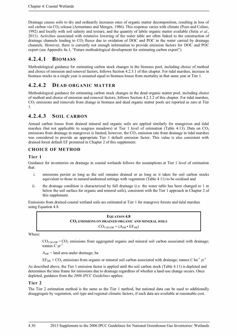
Chapter 4: Coastal Wetlands
4.30 2013 Supplement to the 2006 IPCC Guidelines for National Greenhouse Gas Inventories: Wetlands
Drainage causes soils to dry and ordinarily increases rates of organic matter decomposition, resulting in loss of
soil carbon via CO2 release (Armentano and Menges, 1986). This response varies with climate (Pozo and Colino,
1992) and locally with soil salinity and texture, and the quantity of labile organic matter available (Setia et al., 2011). Activities associated with extensive lowering of the water table are often linked to the construction of
drainage channels leading to CO2 fluxes due to oxidation of DOC and POC in the water carried by drainage
channels. However, there is currently not enough information to provide emission factors for DOC and POC
export (see Appendix 4a.1, “Future methodological development for estimating carbon export”).
4.2.4.1 BIOMASS
Methodological guidance for estimating carbon stock changes in the biomass pool, including choice of method
and choice of emission and removal factors, follows Section 4.2.3.1 of this chapter. For tidal marshes, increase in biomass stocks in a single year is assumed equal to biomass losses from mortality in that same year at Tier 1.
4.2.4.2 DEAD ORGANIC MATTER
Methodological guidance for estimating carbon stock changes in the dead organic matter pool, including choice
of method and choice of emission and removal factors, follows Section 4.2.3.2 of this chapter. For tidal marshes,
CO2 emissions and removals from change in biomass and dead organic matter pools are reported as zero at Tier
1.
4.2.4.3 SOIL CARBON
Annual carbon losses from drained mineral and organic soils are applied similarly for mangroves and tidal
marshes (but not applicable to seagrass meadows) at Tier 1 level of estimation (Table 4.13). Data on CO2
emissions from drainage in mangroves is limited, however, the CO2 emission rate from drainage in tidal marshes
was considered to provide an appropriate Tier 1 default emission factor. This value is also consistent with
drained forest default EF presented in Chapter 2 of this supplement.
CHOICE OF METHOD
Tier 1
Guidance for inventories on drainage in coastal wetlands follows the assumptions at Tier 1 level of estimation
that:
i. emissions persist as long as the soil remains drained or as long as it takes for soil carbon stocks equivalent to those in natural/undrained settings with vegetation (Table 4.11) to be oxidised and
ii. the drainage condition is characterized by full drainage (i.e. the water table has been changed to 1 m
below the soil surface for organic and mineral soils), consistent with the Tier 1 approach in Chapter 2 of
this supplement.
Emissions from drained coastal wetland soils are estimated at Tier 1 for mangrove forests and tidal marshes
using Equation 4.8.
EQUATION 4.8
CO2 EMISSIONS ON DRAINED ORGANIC AND MINERAL SOILS
CO2-SO-DR = (ADR • EFDR)
Where:
CO2-SO-DR = CO2 emissions from aggregated organic and mineral soil carbon associated with drainage;
tonnes C yr-1
ADR = land area under drainage; ha
EFDR, = CO2 emissions from organic or mineral soil carbon associated with drainage; tonnes C ha-1 yr-1
As described above, the Tier 1 emission factor is applied until the soil carbon stock (Table 4.11) is depleted and
determines the time frame for emissions due to drainage regardless of whether a land-use change occurs. Once
depleted, guidance from the 2006 IPCC Guidelines applies.
Tier 2
The Tier 2 estimation method is the same as the Tier 1 method, but national data can be used to additionally
disaggregate by vegetation, soil type and regional climatic factors, if such data are available at reasonable cost.

Chapter 4: Coastal Wetlands
2013 Supplement to the 2006 IPCC Guidelines for National Greenhouse Gas Inventories: Wetlands 4.31
Tier 3
Tier 3 methods could take account of differences in the management of the drained wetland. Empirical
measurements of gas flux based on site-specific measurements of, for example, carbon content, bulk density,
clay content, salinity, redox potential, etc., to determine the underlying processes of emissions could be included.
Site differences in frequency of drainage activity could also be considered at Tier 3 methods. Other factors that
could be used to apply disaggregated data include salinity and tidal export of DOC and POC (Appendix 4a.1).
CHOICE OF EMISSION/REMOVAL FACTORS
Tier 1
At Tier 1, a generic default emission factor is applied for drainage, regardless of vegetation or soil type (Table
4.13). That is, the same EF is applied regardless of the management activity involving soil drainage.
Tier 2
Tier 2 emission factors apply country-specific data disaggregated by soil type, vegetation type, and climate,
where feasible. Data to address any change in emissions since initiation of drainage could additionally be
implemented.
Tier 3
In a Tier 3 approach, field measurements of soil organic carbon content and CO2 emissions from the drained site
would be useful to develop an empirical relationship (for example, a simple regression equation of soil carbon
content versus rate of carbon removal) that can be used across other drained sites within a particular area or
country. Country-specific values can thus be developed to model possible time-dependent changes in CO2
emissions such as changes in relation to timing and rate of soil drainage, depth of drainage and additional national information about mean annual water table and land-use type or intensity. A comprehensive
understanding and representation of the dynamics of CO2 emission factors, based on field measurements of, for
example, carbon content, bulk density, clay content, salinity, redox potential, etc., could be employed at Tier 3.
CHOICE OF ACTIVITY DATA
Tier 1
The Tier 1 approach requires area data of drained land for each land-use category that have been identified in
coastal wetlands. Classification systems for activity data that form the basis for a Tier 1 inventory are provided
in the respective chapters of the 2006 IPCC Guidelines. For coastal wetlands, the predominant land-use category
conversion is to Cropland and Grassland.
Tier 2 and 3
Activity data for higher tier estimates are generally derived following the methods presented in Chapter 3 of the
2006 IPCC Guidelines. To disaggregate by soil type and vegetation type, several institutions, including ISRIC
and FAO have country-specific and global maps that include organic soils
(http://www.fao.org/geonetwork/srv/en/main.home or http://www.isric.org/). A global consortium has been
formed to make a new digital soil map of the world at fine resolution (http://www.globalsoilmap.net/).
Drainage is assumed to result in persistent emissions from soils as long as the management system remains in
place. Activity data may be spatially explicit and could be disaggregated by type of management, if appropriate
emissions factors are available.
The combination of land-use databases and soil maps or spatially-explicit data allow delineation of combinations
of land-use categories, climate domains, and management systems and their changes over time on organic soils.
Information sources about drainage with adequate disaggregation may include that listed below.
TABLE 4.13
ANNUAL EMISSION FACTORS ASSOCIATED WITH DRAINAGE (EFDR) ON AGGREGATED ORGANIC AND MINERAL SOILS
(TONNES C HA-1
YR-1)
Ecosystem EFDR 95%
CI2
Range N
Tidal marshes and mangroves 7.91 5.2, 11.8 1.2-43.9 22
1Sources: Camporese et al., 2008; Deverel and Leighton, 2010; Hatala et al., 2012; Howe et al., 2009; Rojstaczer and Deverel,1993
295% CI of the geometric mean

Chapter 4: Coastal Wetlands
4.32 2013 Supplement to the 2006 IPCC Guidelines for National Greenhouse Gas Inventories: Wetlands
National land-use statistics. Land-use maps and soil maps, maps of water and nature conservation zones
with restrictions for water management, wetlands.
National water management statistics. In most countries, the agricultural land base including croplands is usually surveyed regularly, providing data on distribution of different land-uses and other aspects of
management, often at sub-national, regional level. These statistics may originate, in part, from remote
sensing methods, from which additional information about wetness or periods with seasonal flooding could
be extracted.
Inventory data from a statistically based, plot-sampling system of water table wells, ditches and surface
waters on organic soils. Water table is monitored at specific permanent sample plots either continuously or
on plots that are revisited on a regular basis. It has to be documented that the water data represent the water
table in the organic soil and for what land-use and drainage stratum and that the data cover a representative
period, which represents a multi-year mean annual water table.
Water management plans and documentation from water management installations.
Drainage maps.
UNCERTAINTY ASSESSMENT
Three broad sources of uncertainty exist in estimating emissions and removals from drainage: 1) uncertainties in
land-use and environmental data; 2) uncertainties in the emission/removal factors for Tier 1 or 2 approaches; and
3) model structure/parameter error for Tier 3 model-based approaches, or measurement error/sampling
variability associated with Tier 3 measurement-based inventories. In general, precision of an inventory is
increased and confidence ranges are smaller with more sampling to estimate values for these categories, while
accuracy is more likely to be increased through implementation of higher Tier methods that incorporate country-
specific information.
For Tier 1, the default uncertainty level of emissions/removal factors is the 95% confidence interval in Table 4.13. Countries developing specific emission factors for their inventories at higher tiers should assess the
uncertainty of these factors.
If using aggregate land-use area statistics for activity data (e.g. FAO data), the inventory agency may have to
apply a default level of uncertainty for the land area estimates, for example. It is good practice for the inventory
compiler to derive uncertainties from country-specific activity data instead of using a default level of
uncertainty. Uncertainties in activity data may be reduced through a better national system, such as developing
or extending a ground-based survey with additional sample locations and/or incorporating remote sensing to
provide additional coverage. Uncertainties in activity data and emission/removal factors need to be combined
using an appropriate method, such as simple error propagation equations. Details are given in Chapter 3, Volume
1 of the 2006 IPCC Guidelines and in Chapter 5 of the GPG-LULUCF.
4.3 NON-CO2 EMISSIONS
This section provides methods for estimating the emissions of CH4 emissions from rewetted mangroves and tidal
marshes and N2O from aquaculture use.
4.3.1 CH4 emissions from rewetted soils and created
mangroves and tidal marshes
Rewetting of drained soils, through reconnection of hydrology, shifts microbial decomposition from aerobic to
anaerobic conditions, increasing the potential for CH4 emissions (Harris et al., 2010). In environments where low
salinity also occurs (especially <5 ppt), microbial decomposition of organic matter may result in production of
CH4. However, in soils saturated with seawater, microbial reduction of sulfate to sulfide will generally occur
before methanogens produce CH4 regardless of the organic matter content. A strong inverse relationship between CH4 emissions and salinity of mangrove soils exists (Purvaja and Ramesh, 2001). A review by Poffenbarger et al.
(2011) showed that CH4 emissions decrease as salinity in tidal marshes increases.
Guidance for estimating CH4 emissions associated with rewetting land previously characterised by mangrove
and tidal marsh vegetation differs from that for estimation of CO2 emissions in that, at Tier 1 level of estimation,
the EF remains the same for CH4, regardless of extant vegetation.

Chapter 4: Coastal Wetlands
2013 Supplement to the 2006 IPCC Guidelines for National Greenhouse Gas Inventories: Wetlands 4.33
4.3.1.1 CHOICE OF METHOD
TIER 1
In the case of rewetting of lands that had been previously in an agricultural (or any other drained) land-use
category, the Tier 1 method estimates CH4 emissions without considering the land-use prior to rewetting.
EQUATION 4.9
CH4 EMISSIONS FROM REWETTED SOILS AND CREATED TIDAL MARSHES AND MANGROVES
CH4-SO-REWET = ∑v(AREWET • EFREWET)v
Where:
CH4-SO-REWET = CH4 emissions associated with rewetted and created coastal wetlands by vegetation type
(v); kg CH4 yr-1
AREWET = Area of soil that has been rewetted (including tidal marsh or mangrove wetland creation), by
vegetation type (v); ha
EFREWET = CH4 emissions from mineral and organic soils that have been rewetted by vegetation type (v);
kg CH4 ha-1 yr-1
TIER 2
At Tier 2, country-specific data can be applied. Improved estimates can be produced if country-specific data
could include more disaggregation by salinity and vegetation type.
TIER 3
At Tier 3, country-specific values can be used and developed to model possible time-dependent changes in CH4 emissions. Tier 3 methods may also consider vegetation composition and density, as plants can act as a conduit
for gas exchange between the soil and atmosphere (e.g. Burdick, 1989; Purvaja and Ramesh, 2001; Kristensen et
al., 2008).
4.3.1.2 CHOICE OF EMISSION FACTORS
TIER 1
Tier 1 CH4 emission factors are found in Table 4.14 and should be used in conjunction with Equation 4.9 to
estimate emissions taking into account vegetation type (and associated salinity level). The choice of emission
factor at Tier 1 is differentiated between rewetting by freshwater and brackish water (<18ppt) and saline water
(>18ppt, Annex 4A.1). Rates of CH4 emissions approximate 0 in saline water marshes and mangroves but are
greater than zero in freshwater tidal and brackish marshes and mangroves (Table 4.14). For rewetting that results
in salinities >18 ppt), the Tier 1 assumption is to apply an annual CH4 emission rate = 0. Within each vegetation
type, CH4 emissions are the same regardless of the management activity involving rewetting at Tier 1.
TIER 2
In a Tier 2 approach, country-specific CH4 emissions are encouraged to be used and will provide better estimates based on the salinity of water used to rewet the mangrove or tidal marsh, particularly to determine CH4 emissions
from tidal brackish marshes.
TIER 3
In a Tier 3 approach, field measurements of soil salinity and CH4 emissions from the rewetted site could be used
to develop an empirical relationship (for example, a simple regression equation of salinity versus rate of methane
emission) and applied across other rewetted sites within a particular area or country. Country-specific values can
thus be developed to model possible time-dependent changes in CH4 emissions such as changes in relation to
frequency of tidal inundation, frequency of the rewetting activity and elevation from the water’s edge. Such
considerations would result in more accurate estimation of CH4 emissions.

Chapter 4: Coastal Wetlands
4.34 2013 Supplement to the 2006 IPCC Guidelines for National Greenhouse Gas Inventories: Wetlands
TABLE 4.14
EMISSION FACTORS FOR CH4 (EFREWET) FOR TIER 1 ESTIMATION OF REWETTED LAND PREVIOUSLY VEGETATED
BY TIDAL MARSHES AND MANGROVES
Vegetation Type Salinity (ppt) EFREWET
(kg CH4 ha-1
y-1
)
95% CI4 Range
Tidal freshwater and brackish marsh and
mangrove1
<18 193.72 99.8, 358 10.95-5392
Tidal saline water marsh and mangrove1
>18 03 0-40
1See Annex 4A.1 for salinity-based definitions
2Sources: Keller et al., 2013; Ma et al., 2012; Poffenbarger et al., 2011; Sotomayor et al., 1994; Tong et al., 2010
3Marshes and mangroves with salinities >1 ppt approximate an order of magnitude lower rates than from tidal freshwater and
brackish marsh (as defined here, salinity <18ppt), so a Tier 1 assumption is to apply 0. 495% CI of the geometric mean
4.3.1.3 CHOICE OF ACTIVITY DATA
To estimate emissions using CH4 emission factors refer, in part, to the guidance for rewetting in Section 4.2.3
above. The EF should be applied to the specific type of vegetation that will be reestablished, which is associated
with salinity. When salinity data are not available the type and location of rewetting may be used as a proxy for
salinity. For example, breaching of sea walls and rewetting in an estuarine setting will result in rewetting with
saline waters. If rewetting occurs with freshwater, a salinity of <18ppt is likely. When applying guidance for tidal freshwater marsh, it is good practice to determine the inland boundary for rewetting of tidal freshwater
wetlands as based on national circumstances, and to consistently apply these conditions to identifying these
rewetted lands. If more information is available on salinity concentrations associated with the area being
rewetted, better estimates of CH4 emissions can be determined. Information used for these assessments should be
documented.
4.3.1.4 UNCERTAINTY ASSESSMENT
There have been few empirical measurements of emissions disaggregated by factors such as temperature, tidal frequency or duration of inundation, which introduce uncertainty in global default emission factors. However,
higher tier approaches can take these factors into account to improve estimations. Few reports are available to
give specifics of the types of rewetting activities that may vary geographically. Because activity data may be
limited in terms of delineating salinity boundaries to apply more constrained CH4 emission factors, aggregation
of data to produce Tier 1 emission factors was based upon expert knowledge. There is also uncertainty in the
time, depth of soil affected, and the contribution of vegetation to rate of CH4 loss.
4.3.2 N2O emissions during aquaculture use in mangroves,
tidal marshes and seagrass meadows
The most significant activity contributing to N2O emissions from managed coastal wetlands is aquaculture. One-
third of global anthropogenic N2O emissions are from aquatic ecosystems, and nearly 6% of anthropogenic
N2O−N emission is anticipated to result from aquaculture by 2030 at its current annual rate of growth (Hu et al.,
2012). Shrimp and fish cultivation increases nutrient loads in culture ponds. As opposed to indirect N2O
emissions originating from activities on terrestrial lands or as wastewater treatment, coastal wetland aquaculture
occurs as a direct source of N2O from coastal wetlands, including mangroves and tidal marshes from aquaculture
pond use. In seagrass meadows, this direct N2O source arises from N added to fish cages (e.g. off-shore
installations). While this differentiation should assure no double-counting, it is good practice to evaluate this
assessment considering national circumstances. As such, this new activity fills a gap in the current reporting on direct and indirect sources of N2O emissions. A country can exclude N2O emissions from estimation that occur
during aquaculture activities where no mangroves, tidal marsh or seagrass meadows exist (i.e. outside of coastal
wetland areas).
N2O is emitted as a by-product of the conversion of ammonia (contained in fish urea) to nitrate through
nitrification and nitrate to N2 gas through denitrification (Hu et al., 2012; Annex 4A.5). N2O emissions can
readily be estimated from fish production data.

Chapter 4: Coastal Wetlands
2013 Supplement to the 2006 IPCC Guidelines for National Greenhouse Gas Inventories: Wetlands 4.35
4.3.2.1 CHOICE OF METHOD
TIER 1
N2O emissions from aquaculture ponds can be estimated based on fish/shrimp production of the aquaculture
activity. N2O emission estimation follows a modified form of Equation 11.1 from Chapter 11, Volume 4 of the
2006 IPCC Guidelines and is presented in Equation 4.10.
EQUATION 4.10
DIRECT N2O EMISSIONS FROM AQUACULTURE USE
N2O-NAQ = FF • EFF (based on fish production)
Where:
N2O-NAQ = annual direct N2O-N emissions from aquaculture use; kg N2O-N yr-1
FF = annual fish production; kg fish yr-1
EFF = emission factor for N2O emissions from fish produced; kg N2O-N (kg fish produced)-1
TIER 2
Tier 2 estimation methodology follows that of Tier 1 with the added information provided by country-specific
data.
TIER 3
Tier 3 estimation methodology could include the consideration of fish/shrimp type, type of feed and stocking
density, category of aquaculture (fish/shrimp species or feed stuff), aquaculture use intensity, and impact of environmental factors (e.g. climate zone, season, and salinity).
4.3.2.2 CHOICE OF EMISSION FACTORS
TIER 1
Hu et al. (2012) used the relationship between in-coming nitrogen loads and N2O emissions from wastewater
plants to estimate that 1.8% of the N is emitted as N2O (0.00169 kg N2O-N is emitted per kg fish produced). The EFF is applied during the ‘in use’ phase of aquaculture (Table 4.15). In the construction and discontinued phases,
non-CO2 emissions are assumed negligible with EF=0. At Tier 1, countries could consider applying this EF to
other species groups under aquaculture production. Because the EF is developed for fish, wider application may
introduce additional uncertainty.
TIERS 2 AND 3
Under the Tier 2 method, country specific emission factors for N2O are applied. At Tier 2, these country-specific
emission factors could incorporate a different value for the proportion of N emitted as N2O. For Tier 3 emission
factors, comprehensive understanding and representation of the dynamics based on direct field measurements or
models is involved, which estimates emission factors considering the category of aquaculture (fish/shrimp species or feed stuff), aquaculture use intensity, and impact of environmental factors e.g. climate zone, season,
and salinity.
TABLE 4.15
EMISSION FACTOR (EFF) FOR N2O EMISSION FROM AQUACULTURE USE IN MANGROVES, TIDAL MARSHES AND
SEAGRASS MEADOWS
Default EF
(kg N2O-N per kg fish produced) 95% CI
1 Reference
0.00169 kg N2O-N per kg fish produced 0, 0.0038 Hu et al., 2012
195% CI of the geometric mean.
Note: Approach used by Hu et al. (2012) using N in feed to fish biomass: Hargreaves, 1998; Protein content of fish biomass:
USDA nutrient database for Standard Reference Nutrient Data Laboratory; N content of protein: Nelson and Cox, 2013; N to
N2O conversion: Hu et al., 2013; Kong et al., 2013; Kampschrew et al., 2008; Ahn et al., 2010 (refer to Annex 4A.5)
Chapter 4: Coastal Wetlands
4.36 2013 Supplement to the 2006 IPCC Guidelines for National Greenhouse Gas Inventories: Wetlands
4.3.2.3 CHOICE OF ACTIVITY DATA
Data for fish and shrimp production are needed. These data can be obtained from FAO
(http://www.fao.org/fishery/statistics/global-aquaculture-production/en). For additional guidance, see Section
4.2.1.
4.3.2.4 UNCERTAINTY ASSESSMENT
Emission factors for N2O emissions from aquaculture systems are based on protein content of fish, relationships
between total nitrogen content and wet weight of fish and the percent of nitrogen load emitted as N2O. There are
no such data for shrimp production so using fish data as a proxy adds a high level of uncertainty. The fish-related
factors can vary greatly, and in part on environmental conditions, so high variation can occur among fish
aquaculture systems. Decreased uncertainty can be achieved at Tier 2 and 3 to reflect variability in N2O
emissions based on shrimp and fish species and type of food (pellets vs. trash fish). Uncertainties in N2O
emissions associated with stocking of aquaculture facilities can be reduced greatly by better estimation of shrimp and fish production.
4.4 COMPLETENESS, TIME SERIES
CONSISTENCY, AND QUALITY ASSURANCE
AND QUALITY CONTROL (QA/QC)
4.4.1 Completeness
General guidance on completeness is provided in Chapter 7 of this supplement.
4.4.2 Time series consistency
It is good practice that countries clearly define coastal wetlands and use this definition consistently over time.
Consistent time series require that the same methodology is used for the entire time series. Whenever new methodologies are used previous estimates should be recalculated using the new methods for all years in the time
series. It is also good practice to report why the new estimates are regarded as more accurate or less uncertain.
One potential problem in recalculating previous estimates is that certain data sets may not be available for the
earlier years. There are several ways of overcoming this limitation and they are explained in detail in Chapter 5,
Volume 1 of the 2006 IPCC Guidelines. Time series consistency is discussed further in Chapter 7.6 of the
Wetlands Supplement and Chapter 5 (Time series consistency and recalculations), Volume 1 of the 2006 IPCC
Guidelines.
4.4.3 Quality Assurance/Quality Control (QA/QC)
Quality assurance/quality control (QA/QC) procedures should be developed and implemented as outlined in
Chapter 7 of this supplement.

Chapter 4: Coastal Wetlands
2013 Supplement to the 2006 IPCC Guidelines for National Greenhouse Gas Inventories: Wetlands 4.37
Annex 4A.1 Salinity-based definitions
SALINITY-BASED DEFINTIONS
Common
description
Salinity (ppt)1
Tidal fresh water <0.5
Brackish water 0.5 - 18
Saline water >18
1ppt is parts per thousand (‰) and is roughly
equivalent to grams of salt per litre of water

Chapter 4: Coastal Wetlands
4.38 2013 Supplement to the 2006 IPCC Guidelines for National Greenhouse Gas Inventories: Wetlands
Annex 4A.2 Estimation of above-ground mangrove biomass:
higher tier methodology
Because of field conditions and heavy weight of wood, an accurate survey of a mangrove forest is difficult and time-consuming. Allometric methods (Soares and Schaeffer-Novelli, 2005; Komiyama et al., 2008) estimate the
whole or partial weight of a tree from measurable tree dimensions, notably trunk diameter and height, using
allometric relations developed from empirical measurement of weight of individual tree components (leaves,
branches, stem). Use of allometric equations is favored because it is non-destructive and is therefore useful for
estimating temporal changes in forest biomass by means of subsequent stem diameter measurements over
subsequent years.
Up until recently, the major drawback of this method has been the site- and species-specific differences in
allometric relations, necessitating the use of different allometric equations for different sites (e.g. Smith and
Whelan, 2005) and, at a minimum, different species. However, a number of workers, using global datasets, have
developed a common allometric equation applicable for all tropical tree species, with the most applicable
equations for above-ground biomass being those developed for all tropical trees by Chave et al. (2005) and for all mangrove species by Komiyama et al. (2005):
Wtop = 0.168pDBH2.47 (Chave et al. 2005)
Wtop = 0.251pD2.46 (Komiyama et al. 2005)
where Wtop = above-ground tree weight in kg dry weight, p = wood specific gravity, D = tree diameter, and DBH
= diameter-at-breast height. The relative error of each equation varies among species, but is typically within the
range of -10% to +10%. There are, of course, arguments to be made that empirical measurements should be
made in all mangrove forests, considering the significant allometric differences between species and for the same
species at different locations (Smith and Whelan, 2005; Soares and Schaeffler-Novelli, 2005). However, this
idea is impractical for inventory compliers; a relative error of ± 10% is acceptable being within the range of error
for allometric relations within a forest where biomass has been weighted.
Comparing the two equations, the Chave estimation gives lower above-ground weight estimates than that of the
Komiyama equation. Presuming that a complete census of all trees, with species identified, and their diameter have been undertaken from replicate plots within a given forest, these numbers can then be used in either
equation to derive individual tree weight.

Chapter 4: Coastal Wetlands
2013 Supplement to the 2006 IPCC Guidelines for National Greenhouse Gas Inventories: Wetlands 4.39
Annex 4A.3 Wood density of mangrove species
WOOD DENSITY OF MANGROVE SPECIES
Species n Average density
(tonnes m-3
) Standard
error
Brugueria gymnorrhiza 8 0.81 0.07
Xylocarpus granatum 7 0.61 0.04
Sonneratia apetala 2 0.50 0.01
Sonneratia alba 6 0.47 0.12
Rhizophora mucronata 9 0.83 0.05
Rhizophora mangle 7 0.87 0.02
Rhizophora apiculata 4 0.87 0.06
Laguncularia racemosa 3 0.60 0.01
Heritiera littoralis 6 0.84 0.05
Heritiera fomes 3 0.86 0.14
Excoecaria agallocha 7 0.41 0.02
Ceriops tagal 7 0.85 0.04
Ceriops decandra 2 0.87 0.10
Avicennia officinalis 3 0.63 0.02
Avicennia marina 6 0.62 0.06
Avicennia germinans 5 0.72 0.04
Average 0.71 0.02
Source: Global Wood Density Database
http://datadryad.org/resource/doi:10.5061/dryad.234/1?show=full; Saenger, 2002; Komiyama et al., 2005;
Donato et al., 2012

Chapter 4: Coastal Wetlands
4.40 2013 Supplement to the 2006 IPCC Guidelines for National Greenhouse Gas Inventories: Wetlands
Annex 4A.4 Percent refractory carbon
Percent refractory carbon in organic/mineral soils were estimated for mangrove soils based on either the amount
of phenolic compounds/lignins in soils or % TOC in mangrove soils deeper than 1 m if there was no further
decline in TOC concentration.
PERCENT REFRACTORY CARBON APPLIED TO
ESTIMATE % C OXIDATION FOR MANGROVE
SOILS (% BY SOIL DRY WEIGHT)
Mean 3.98
Median 3.4
N 16
Source: Prasad and Ramanathan, 2009; Marchand et al.,
2003; Dittmar and Lara, 2001; Koch et al., 2011;
Ranjan et al., 2010; Marchand et al., 2005, which is
similar to that in tidal marshes (Filip et al., 1988; Alberts et al., 1988; Reddy and DeLaune, 2008).

Chapter 4: Coastal Wetlands
2013 Supplement to the 2006 IPCC Guidelines for National Greenhouse Gas Inventories: Wetlands 4.41
Annex 4A.5 Derivation of N2O emission factor for aquaculture
The emission factor of 0.00169 kg N20-N per kg fish produced in Table 4.15 is based on the following. Firstly,
the protein content of fish is estimated from 80 values in various cultured fish species as 17.72 ± 2.97% (USDA
nutrient database for Standard Reference Nutrient Data Laboratory). Using the protein content of fish and the
average N content of protein (16%; Nelson and Cox, 2013) implies an N content of 2.84 ± 1.33% of fish biomass; i.e. one metric tonne of fish contains 2.84 x 10
4 g N. Secondly, the % N in aquaculture fish feed that is
incorporated into fish biomass averages 23.22 ± 5.88% (Hargreaves, 1998). This value is based on results from
four aquaculture production methods in which 18 individual estimates for the conversion of fish biomass to fish
N were obtained from 11 different cultured fish species.
Following Hu et al. (2012; and references therein), it is assumed that all the feed is ingested by fish and the N
input as ammonia to the aqueous phase to produce 1 metric tonne of fish is 12.23 x 10⁴ g - 2.84 x 10⁴ g = 9.39 ±
4.69 x 10⁴ g. Given that on average, during N transformation in the aqueous phase, 1.8 ± 0.7% of the N is
converted to N2O (Kong et al., 2013; Kampschreur et al., 2008; Ahn et al., 2010; Hu et al., 2013), the amount of
N emitted to the atmosphere as N2O-N is 1.69 x 10³ g. Thus the average N2O emission factor of an aquaculture
system is 1.69 g N2O-N per kg fish or 0.00169 kg N2O-N per kg fish produced. The uncertainty range is
estimated using standard error propagation through the calculations indicated.
Chapter 4: Coastal Wetlands
4.42 2013 Supplement to the 2006 IPCC Guidelines for National Greenhouse Gas Inventories: Wetlands
Appendix 4a.1 Future methodological development for estimating
carbon export
The amount of dissolved and particulate carbon potentially available for export is highly variable among coastal wetlands, depending on a large number of factors such as: net primary productivity, tidal range, the ratio of
wetland to watershed area, lateral trapping of tidal water, the presence of high salinity plugs in the tropical dry
season, total wetland area, frequency of storms, amount of precipitation, and volume of water exchange. Each
ecosystem is unique; some wetlands export DOC but import POC, others import DOC and POC but export DIC,
while other systems import or export all forms of dissolved and particulate C. The direction of net exchange also
usually varies within the same estuary with change in season. Emerging evidence indicates that DIC (derived
from CO2 by heterotrophic organisms and/or carbonate dissolution) is exported from coastal wetlands by the
physical processes of tidal drainage of soils and subsequent advection to adjacent waterways (Alongi, 2009;
Perillo et al., 2009). For instance, in mangroves, tidal export of respiratory-derived DIC may equate to as much
as one-third of carbon fixed by the forests. However, available data are still too few to allow for generalization,
and the scant data are highly variable with tidal amplitude being a major driver of soil DIC drainage.
Estimation of tidal exchange in a particular wetland is not a straightforward process. Many workers have
provided rough estimates by multiplying carbon concentrations suspended in wetland creeks and waterways by
the tidal range multiplied by the creek/waterway cross-sectional area. Estimates derived from such simple
calculations are invalid and misleading for a number of reasons, including the inherent assumption that there are
differences in carbon concentrations between ebb and flood tide stages and that the tidal prism is symmetrical. In
fact, carbon concentrations in many wetland waters do not show significant differences between tides. Further,
tides in most wetlands are characterized by a pronounced asymmetry between ebb and flood tides with the ebb
most often being of shorter duration but with stronger current velocity than the flood tide. Also, tidal velocities
vary across a waterway with faster surface current velocities mid-stream than those just above the creekbed or
proximal to the wetland.
For these reasons, it is not possible to make simple generalizations regarding dissolved and particulate organic
and inorganic total carbon export from mangroves, seagrasses or tidal marshes and, in fact, comparatively few such measurements have been made properly. The correct method would be to measure water volume and
velocity over entire tidal cycles over several seasons in relation to position in the water-column to derive an
overall annual estimate of average water flow by volume. This involves fairly complex instrument measurements
and sophisticated mathematical modelling as well as extensive and expensive repetitive measurements of
dissolved and particulate carbon concentrations. For mangroves, net exchange of carbon has been properly
measured in only twelve systems (DIC has only been measured in four systems), with no clear exchange patterns
among locations, although it does appear that most mangroves export POC as litter but with rates ranging widely
from 0.1-27.7 mol C m-2 yr-1 (Alongi, 2009). This export equates globally to only about 10% of total carbon fixed
by trees; respiration to the atmosphere is by far the largest loss of carbon to the atmosphere. Such appears to be
the case for tidal marshes (Chmura et al., 2003) and subtidal seagrass beds (Fourqurean et al., 2012). Some
recent syntheses and literature do hold promise for future development of model relationships that can be used for estimating carbon export (Adame and Lovelock 2011; Maher et al., 2013).
Chapter 4: Coastal Wetlands
2013 Supplement to the 2006 IPCC Guidelines for National Greenhouse Gas Inventories: Wetlands 4.43
References
Abohassan, R. A. A., Okia, C. A., Agea, J. G., Kimondo, J. M. & McDonald, M. M. (2012) Perennial biomass
production in arid mangrove systems on the Red Sea coast of Saudi Arabia. Environmental Research Journal
6(1): 22-31.
Adame, M. C., and C.E. Lovelock (2011) Carbon and nutrient exchange of mangrove forests with the coastal ocean. Hydrobiologia 663: 23-50.
Adame, M. F., Reef, R., Herrera-Silveira, J. A. & Lovelock, C. E. (2012) Sensitivity of dissolved organic carbon
exchange and sediment bacteria to water quality in mangrove forests. Hydrobiologia 691(1): 239-253.
Adams, C. A., Andrews, J. E. & Jickells, T. (2012) Nitrous oxide and methane fluxes vs. carbon, nitrogen and
phosphorous burial in new intertidal and saltmarsh sediments. Science of the Total Environment 434: 240-
251.
Agostini, S., Pergent, G. & Marchand, B. (2003) Growth and primary production of Cymodocea nodosa in a
coastal lagoon. Aquatic Botany 76(3): 185-193.
Ahn, J. H., Kwan, T. & Chandran, K. (2011) Comparison of partial and full nitrification processes applied for
treating high-strength nitrogen wastewaters: microbial ecology through nitrous oxide production.
Environmental Science & Technology 45: 2734-2740.
Aioi, K. (1980) Seasonal change in the standing crop of eelgrass Zostera marina in Odawa Bay, Central Japan.
Aquatic Botany 8(4): 343-354.
Aioi, K., Mukai, H., Koike, I., Ohtsu, M. & Hattori, A. (1981) Growth and organic production of eelgrass
Zostera-marina in temperate waters of the Pacific coast of Japan. 2.Growth Analysis in Winter. Aquatic
Botany 10(2): 175-182.
Aioi, K. & Pollard, P. C. (1993) Biomass, Leaf growth and loss rate of the seagrass Syringodium isotifolium on
Dravuni Island, Fiji. Aquatic Botany 46(3-4): 283-292.
Ajonina, G. M. (2008) Inventory and modelling mangrove forest stand dynamics following different levels of
wood exploitation pressures in the Douala-Edea Atlantic Coast of Cameroon, Central Africa, Freiburg im
Breisgau, Germany, p. 232.
Alberts, J. J., Filip, Z., Price, M. T., Williams, D. J. & Williams, M. C. (1988) Elemental composition, stable
carbon isotope ratios and spectrophotometric properties of humic substances occurring in a salt-marsh estuary. Organic Geochemistry 12(5): 455-467.
Allen, J. A., Ewel, K. C., Keeland, B. D., Tara, T. & Smith, T. J. (2000) Downed wood in Micronesian
mangrove forests. Wetlands 20(1): 169-176.
Alongi, D. M. (2010) The Energetics of Mangrove Forests. Dordrecht, Netherlands: Springer Science+Business
Media B.V.
Alongi, D. M., Clough, B. F., Dixon, P. & Tirendi, F. (2003) Nutrient partitioning and storage in arid-zone
forests of the mangroves Rhizophora stylosa and Avicennia marina. Trees-Structure and Function 17(1): 51-
60.
Alongi, D. M., McKinnon, A. D., Brinkman, R., Trott, L. A., Undu, M. C., Muawanah & Rachmansyah. (2009)
The fate of organic matter derived from small-scale fish cage aquaculture in coastal waters of Sulawesi and
Sumatra, Indonesia. Aquaculture 295(1-2): 60-75.
Amarasinghe, M. D. & Balasubramaniam, S. (1992) Net primary productivity of two mangrove forest stands on
the Northwestern coast of Sri-Lanka. Hydrobiologia 247(1-3): 37-47.
Anisfeld, S. C., Tobin, M. & Benoit, G. (1999) Sedimentation rates in flow-restricted and restored salt marshes
in Long Island Sound. Estuaries 22(2A): 231-244.
Armentano, T. V. a. M., E.S. (1986) Patterns of change in the carbon balance of organic soil wetlands of the
temperate zone. Journal of Ecology 74: 755-774.
Asmus, R. M., Sprung, M. & Asmus, H. (2000) Nutrient fluxes in intertidal communities of a South European
lagoon (Ria Formosa) - similarities and differences with a northern Wadden Sea bay (Sylt-Romo Bay).
Hydrobiologia 436(1-3): 217-235.
Bandeira, S. O. (2002) Leaf production rates of Thalassodendron ciliatum from rocky and sandy habitats.
Aquatic Botany 72(1): 13-24.

Chapter 4: Coastal Wetlands
4.44 2013 Supplement to the 2006 IPCC Guidelines for National Greenhouse Gas Inventories: Wetlands
Bank, W. (2006) Aquaculture: Changing the Face of the Waters Meeting the Promise and Challenge of
Sustainable Aquaculture.
Birch, J. B. & Cooley, J. L. (1982) Production and standing crop patterns of giant cutgrass Zizaniopsis miliacea in a freshwater tidal marsh. Oecologia 52(2): 230-235.
Blackburn, T. H., Lund, B. A. & Krom, M. D. (1988) C-mineralization and N-mineralization in the sediments of
earthen marine fishponds. Marine Ecology Progress Series 44(3): 221-227.
Boon, P. I. (1986) Nitrogen pools in seagrass beds of Cymodocea serrulata and Zostera capricorni of Moreton
Bay, Australia. Aquatic Botany 25(1): 1-19.
Borum, J., Duarte, C. M., Krause-Jensen, D. & Greve, T. M. (2004) European seagrasses: an introduction to
monitoring and management. In: The M&MS project.
Bouillon, S., Borges, A. V., Castaneda-Moya, E., Diele, K., Dittmar, T., Duke, N. C., Kristensen, E., Lee, S. Y.,
Marchand, C., Middelburg, J. J., Rivera-Monroy, V. H., Smith, T. J. & Twilley, R. R. (2008) Mangrove
production and carbon sinks: A revision of global budget estimates. Global Biogeochemical Cycles 22(2).
Boyer, K. E., Callaway, J. C. & Zedler, J. B. (2000) Evaluating the progress of restored cordgrass Spartina foliosa marshes: Below-ground biomass and tissue nitrogen. Estuaries 23(5): 711-721.
Breithaupt, J. L., Smoak, J. M., Smith, T. J., Sanders, C. J. & Hoare, A. (2012) Organic carbon burial rates in
mangrove sediments: Strengthening the global budget. Global Biogeochemical Cycles 26.
Briggs, S. V. (1977) Estimates of biomass in a temperate mangrove community. Australian Journal of Ecology
2(3): 369-373.
Brouns, J. (1985) A comparison of the annual production and biomass in three monospecific stands of the
seagrass Thalassia hemprichii (Ehrenb) Aschers. Aquatic Botany 23(2): 149-175.
Brouns, J. (1987) Aspects of production and biomass of four seagrass species Cymodoceoideae from Papua New
Guinea. Aquatic Botany 27(4): 333-362.
Brouns, J. & Heijs, F. M. L. (1986) Production and biomass of the seagrass Enhalus acoroides (L.f.) Royle and
its epiphytes. Aquatic Botany 25(1): 21-45.
Brun, F. G., van Zetten, E., Cacabelos, E. & Bouma, T. J. (2009) Role of two contrasting ecosystem engineers Zostera noltii and Cymodocea nodosa on the food intake rate of Cerastoderma edule. Helgoland Marine
Research 63(1): 19-25.
Cahoon, D. R., Lynch, J. C. & Knaus, R. M. (1996) Improved cryogenic coring device for sampling wetland
soils. Journal of Sedimentary Research 66(5): 1025-1027.
Callaway, J. C., R.D. DeLaune, and W.H. Patrick. (1997) Sediment accretion rates from four coastal wetlands
along the Gulf of Mexico. Journal of Coastal Research 13: 181-191.
Callaway, J. C., Borgnis, E. L., Turner, R. E. & Milan, C. S. (2012) Carbon sequestration and sediment accretion
in San Francisco Bay tidal wetlands. Estuaries and Coasts 35(5): 1163-1181.
Callaway, J. C., DeLaune, R. D. & Patrick, W. H. (1996) Chernobyl Cs-137 used to determine sediment
accretion rates at selected northern European coastal wetlands. Limnology and Oceanography 41(3): 444-450.
Calleja, M. L., Barron, C., Hale, J. A., Frazer, T. K. & Duarte, C. M. (2006) Light regulation of benthic sulfate reduction rates mediated by seagrass Thalassia testudinum metabolism. Estuaries and Coasts 29(6B): 1255-
1264.
Camacho, L. D., Gevaña, D. T., Carandang, A. P., Camacho, S. C., Combalicer, E. A., Rebugio, L. L. & Youn,
Y.-C. (2011) Tree biomass and carbon stock of a community‐managed mangrove forest in Bohol, Philippines.
Forest Science and Technology 7(4): 161-167.
Camporese, M., Putti, M., Salandin, P. & Teatini, P. (2008) Spatial variability of CO2 efflux in a drained
cropped peatland south of Venice, Italy. Journal of Geophysical Research-Biogeosciences 113(G4).
Cebrian, J., Pedersen, M. F., Kroeger, K. D. & Valiela, I. (2000) Fate of production of the seagrass Cymodocea
nodosa in different stages of meadow formation. Marine Ecology Progress Series 204: 119-130.
Chave, J., Andalo, C., Brown, S., Cairns, M. A., Chambers, J. Q., Eamus, D., Folster, H., Fromard, F., Higuchi,
N., Kira, T., Lescure, J. P., Nelson, B. W., Ogawa, H., Puig, H., Riera, B. & Yamakura, T. (2005) Tree allometry and improved estimation of carbon stocks and balance in tropical forests. Oecologia 145(1): 87-99.
Chen, G. C., Ye, Y. & Lu, C. Y. (2008) Seasonal variability of leaf litter removal by crabs in a Kandelia candel
mangrove forest in Jiulong Jiang Estuary, China. Estuarine Coastal and Shelf Science 79(4): 701-706.

Chapter 4: Coastal Wetlands
2013 Supplement to the 2006 IPCC Guidelines for National Greenhouse Gas Inventories: Wetlands 4.45
Chmura, G. L., Anisfeld, S. C., Cahoon, D. R. & Lynch, J. C. (2003) Global carbon sequestration in tidal, saline
wetland soils. Global Biogeochemical Cycles 17(4).
Chmura, G. L. & Hung, G. A. (2004) Controls on salt marsh accretion: A test in salt marshes of Eastern Canada. Estuaries 27(1): 70-81.
Christensen, B. (1978) Biomass and primary production of Rhizophora apiculata Bl. in a mangrove in southern
Thailand. Aquatic Botany 4(1): 43-52.
Coles, R. G., Long, W. J. L., Watson, R. A. & Derbyshire, K. J. (1993) Distribution of Seagrasses, and Their
Fish and Penaeid Prawn Communities, in Cairns Harbour, a Tropical Estuary, Northern Queensland,
Australia. Australian Journal of Marine and Freshwater Research 44(1): 193-210.
Collier, C. J., Lavery, P. S., Ralph, P. J. & Masini, R. J. (2009) Shade-induced response and recovery of the
seagrass Posidonia sinuosa. Journal of Experimental Marine Biology and Ecology 370(1-2): 89-103.
Connor, R. & Chmura, G. L. (2000) Dynamics of above- and below-ground organic matter in a high latitude
macrotidal saltmarsh. Marine Ecology Progress Series 204: 101-110.
Connor, R. F., Chmura, G. L. & Beecher, C. B. (2001) Carbon accumulation in Bay of Fundy salt marshes: Implications for restoration of reclaimed marshes. Global Biogeochemical Cycles 15(4): 943-954.
Coronado-Molina, C., Day, J., Reyes, E. & Perez, B. (2004) Standing crop and aboveground biomass
partitioning of a dwarf mangrove forest in Taylor River Slough, Florida. Wetlands Ecology and Management
12(3): 157-164.
Craft, C., J. Reader, J.N. Sacco, S.W. Broome. (1999) Twenty-five years of ecosystem development of
constructed Spartina alterniflora (Loisel) marshes. Ecological Applications 13: 1417-1423.
Craft, C., S. Broome, and C. Campbell. (2002) Fifteen years of vegetation and soil developent after brackish-
water marsh creation. Restoration Ecology (10): 248-258.
Craft, C. (2007) Freshwater input structures soil properties, vertical accretion, and nutrient accumulation of
Georgia and U.S. tidal marshes. Limnology and Oceanography 52(3): 1220-1230.
Craft, C., Megonigal, P., Broome, S., Stevenson, J., Freese, R., Cornell, J., Zheng, L. & Sacco, J. (2003) The
pace of ecosystem development of constructed Spartina alterniflora marshes. Ecological Applications 13(5): 1417-1432.
Craft, C. B., Broome, S. W. & Seneca, E. D. (1988) Nitrogen, phosphorus and organic carbon pools in natural
and transplanted marsh soils. Estuaries 11(4): 272-280.
Cruz, P. S. (1997) Aquaculture feed and fertilizer resource atlas of the Philippines. FAO.
da Cunha Lana, P., Guiss, C. & Disaro, S. T. (1991) Seasonal variation of biomass and production dynamics for
above- and below-ground components of a Spartina alterniflora marsh in the euhaline sector of Paranagua
Bay (SE Brazil). Estuarine Coastal and Shelf Science 32: 231-241.
Daby, D. (2003) Effects of seagrass bed removal for tourism purposes in a Mauritian bay. Environmental
Pollution 125(3): 313-324.
de Boer, W. F. (2000) Biomass dynamics of seagrasses and the role of mangrove and seagrass vegetation as
different nutrient sources for an intertidal ecosystem. Aquatic Botany 66(3): 225-239.
Deverel, S. J. & Leighton, D. A. (2010) Historic, recent, and future subsidence, Sacramento-San Joaquin Delta,
California, USA. . San Francisco Estuary and Watershed Science 8(2): 1-23.
Devereux, R., Yates, D. F., Aukamp, J., Quarles, R. L., Jordan, S. J., Stanley, R. S. & Eldridge, P. M. (2011)
Interactions of Thalassia testudinum and sediment biogeochemistry in Santa Rosa Sound, NW Florida.
Marine Biology Research 7(4): 317-331.
Dittmar, T. & Lara, R. J. (2001) Molecular evidence for lignin degradation in sulfate-reducing mangrove
sediments (Amazonia, Brazil). Geochimica Et Cosmochimica Acta 65(9): 1417-1428.
Dixon, L. K. & Leverone, J. R. (1995) Light requirements of Thalassia testudinum in Tampa Bay, Florida: final
report.
Donato, D. C., Kauffman, J. B., Mackenzie, R. A., Ainsworth, A. & Pfleeger, A. Z. (2012) Whole-island carbon
stocks in the tropical Pacific: Implications for mangrove conservation and upland restoration. Journal of
Environmental Management 97: 89-96.
Donato, D. C., Kauffman, J. B., Murdiyarso, D., Kurnianto, S., Stidham, M. & Kanninen, M. (2011) Mangroves
among the most carbon-rich forests in the tropics. Nature Geoscience 4(5): 293-297.

Chapter 4: Coastal Wetlands
4.46 2013 Supplement to the 2006 IPCC Guidelines for National Greenhouse Gas Inventories: Wetlands
Dos Santos, V. M., Matheson, F. E., Pilditch, C. A. & Elger, A. (2012) Is black swan grazing a threat to seagrass?
Indications from an observational study in New Zealand. Aquatic Botany 100: 41-50.
Duarte, C. M., Kennedy, H., Marbà, N. & Hendriks, I. (2013) Assessing the capacity of seagrass meadows for carbon burial: current limitations and future strategies. Ocean and Coastal Management 83: 32-38.
Dunn, R. (1981) The effects of temperature on the photosynthesis, growth and productivity of Spartina
townsendu (sensu lato) in controlled and natural environments. In: University of Essex.
Dunton, K. H. (1996) Photosynthetic production and biomass of the subtropical seagrass Halodule wrightii along
an estuarine gradient. Estuaries 19(2B): 436-447.
Dürr, H. H., Laruelle, G. G., van Kempen, C. M., Slomp, C. P., Meybeck, M. & Middelkoop, H. (2011) World-
wide typology of near-shore coastal systems: defining the estuarine filter of river inputs to the oceans.
Estuaries and Coasts 34(3): 441-458.
Ellison, A. M., Bertness, M. D. & Miller, T. (1986) Seasonal patterns in the below-ground biomass of Spartina
alterniflora (Gramineae) across a tidal gradient. American Journal of Botany 73(11): 1548-1554.
Ellison, A. M. & Farnsworth, E. J. (1996) Anthropogenic disturbance of Caribbean mangrove ecosystems: Past impacts, present trends, and future predictions. Biotropica 28(4): 549-565.
Elsey-Quirk, T., Seliskar, D. M., Sommerfield, C. K. & Gallagher, J. L. (2011) Salt Marsh Carbon Pool
Distribution in a Mid-Atlantic Lagoon, USA: Sea Level Rise Implications. Wetlands 31(1): 87-99.
FAO. (2003) Status and trends in mangrove area extent worldwide. In: Paris: Food and Agriculture Organization
of the United Nations
FAO. (2007) The State of the World Fisheries and Aquaculture 2006. In: Rome: FAO Fisheries and Aquaculture
Department, Food and Agriculture Organisation of the United Nations.
FAO. (2007) The world's mangroves 1980-2005: a thematic study prepared in the framework of the Global
Forest Resources Assessment 2005. In: Rome: Food and Agriculture Organisation of the United Nations.
Fatoyinbo, T. E. & Simard, M. (2013) Height and biomass of mangroves in Africa from ICESat/GLAS and
SRTM. International Journal of Remote Sensing 34(2): 668-681.
Fatoyinbo, T. E., Simard, M., Washington-Allen, R. A. & Shugart, H. H. (2008) Landscape-scale extent, height, biomass, and carbon estimation of Mozambique's mangrove forests with Landsat ETM+ and Shuttle Radar
Topography Mission elevation data. Journal of Geophysical Research-Biogeosciences 113(G2).
Filip, Z., Alberts, J. J., Cheshire, M. V., Goodman, B. A. & Bacon, J. R. (1988) Comparison of salt marsh humic
acid with humic-like substances from the indigenous plant species Spartina alterniflora (Loisel). Science of
the Total Environment 71(2): 157-172.
Fourqurean, J. W., Duarte, C. M., Kennedy, H., Marba, N., Holmer, M., Mateo, M. A., Apostolaki, E. T.,
Kendrick, G. A., Krause-Jensen, D., McGlathery, K. J. & Serrano, O. (2012) Seagrass ecosystems as a
globally significant carbon stock. Nature Geoscience 5(7): 505-509.
Fourqurean, J. W., Moore, T. O., Fry, B. & Hollibaugh, J. T. (1997) Spatial and temporal variation in C:N:P
ratios, delta N-15 and delta C-13 of eelgrass Zostera marina as indicators of ecosystem processes, Tomales
Bay, California, USA. Marine Ecology Progress Series 157: 147-157.
Fromard, F., Puig, H., Mougin, E., Marty, G., Betoulle, J. L. & Cadamuro, L. (1998) Structure, aboveground
biomass and dynamics of mangrove ecosystems: new data from French Guiana. Oecologia 115(1-2): 39-53.
Fujimoto, K., Imaya, A., Tabuchi, R., Kuramoto, S., Utsugi, H. & Murofushi, T. (1999) Below-ground carbon
storage of Micronesian mangrove forests. Ecological Research 14(4): 409-413.
Gedan, K. B., Silliman, B. R. & Bertness, M. D. (2009) Centuries of human-driven change in salt marsh
ecosystems. Annual Review of Marine Science 1: 117-141.
Golley, F. B., McGuiniss, K., Clements, R. G., Child, G. I. & Duever, M. J. (1975) Mineral cycling in a tropical
moist ecosystem. Athens, GA, USA: University of Georgia Press.
Golley, F. B., Odum, H. T. & Wilson, R. F. (1962) The structure and metabolism of a Puerto Rican red
mangrove forest ecosystem. Athens, GA, USA: University of Georgia Press.
Gong, W. K. & Ong, J. E. (1990) Plant biomass and nutrient flux in a managed mangrove forest in Malaysia.
Estuarine Coastal and Shelf Science 31(5): 519-530.
Gross, M. F., Hardisky, M. A., Wolf, P. L. & Klemas, V. (1991) Relationship between aboveground and below-
ground biomass of Spartina alterniflora (smooth cordgrass). Estuaries 14(2): 180-191.

Chapter 4: Coastal Wetlands
2013 Supplement to the 2006 IPCC Guidelines for National Greenhouse Gas Inventories: Wetlands 4.47
Hackney, J. W. (2003) Morphometric variability and allometric relationships in the seagrass Thalassia
testudinum in Florida Bay. In: University of North Carolina.
Halun, Z., Terrados, J., Borum, J., Kamp-Nielsen, L., Duarte, C. M. & Fortes, M. D. (2002) Experimental evaluation of the effects of siltation-derived changes in sediment conditions on the Philippine seagrass
Cymodocea rotundata. Journal of Experimental Marine Biology and Ecology 279(1-2): 73-87.
Hargreaves, J. A. (1998) Nitrogen biogeochemistry of aquaculture ponds. Aquaculture 166: 181-212.
Harris, R. J., Milbrandt, E. C., Everham, E. M. & Bovard, B. D. (2010) The Effects of Reduced Tidal Flushing
on Mangrove Structure and Function Across a Disturbance Gradient. Estuaries and Coasts 33(5): 1176-1185.
Hatala, J. A., Detto, M., Sonnentag, O., Deverel, S. J., Verfaillie, J. & Baldocchi, D. D. (2012) Greenhouse gas
(CO2, CH4, H2O) fluxes from drained and flooded agricultural peatlands in the Sacramento-San Joaquin
Delta. Agriculture Ecosystems & Environment 150: 1-18.
Hatton, R. S., Delaune, R. D. & Patrick, W. H. (1983) Sedimentation, accretion, and subsidence in marshes of
Barataria Basin, Louisiana. Limnology and Oceanography 28(3): 494-502.
Hebert, A. B., Morse, J. W. & Eldridge, P. M. (2007) Small-scale heterogeneity in the geochemistry of seagrass vegetated and non-vegetated estuarine sediments: causes and consequences. Aquatic Geochemistry 13(1): 19-
39.
Herbert, D. A. (1986) The growth dynamics of Halophila hawaiiana. Aquatic Botany 23(4): 351-360.
Herbert, D. A. & Fourqurean, J. W. (2008) Ecosystem structure and function still altered two decades after short-
term fertilization of a seagrass meadow. Ecosystems 11(5): 688-700.
Herbert, D. A. & Fourqurean, J. W. (2009) Phosphorus Availability and Salinity Control Productivity and
Demography of the Seagrass Thalassia testudinum in Florida Bay. Estuaries and Coasts 32(1): 188-201.
Holmer, M., Andersen, F. O., Nielsen, S. L. & Boschker, H. T. S. (2001) The importance of mineralization based
on sulfate reduction for nutrient regeneration in tropical seagrass sediments. Aquatic Botany 71(1): 1-17.
Holmer, M. & Kendrick, G. A. (2013) High sulfide intrusion in five temperate seagrasses growing under
contrasting sediment conditions. Estuaries and Coasts 36(1): 116-126.
Hoque, A., Sharma, S., Suwa, R., Mori, S. & Hagihara, A. (2012) Seasonal variation in the size-dependent respiration of mangroves Kandelia obovata. Marine Ecology Progress Series 404: 31-37.
Howe, A. J., Rodriguez, J. F. & Saco, P. M. (2009) Surface evolution and carbon sequestration in disturbed and
undisturbed wetland soils of the Hunter estuary, southeast Australia. Estuarine Coastal and Shelf Science
84(1): 75-83.
Hu, Z., Lee, J. W., Chandran, K., Kim, S. & Khanal, S. K. (2012) Nitrous Oxide (N2O) Emission from
Aquaculture: A Review. Environmental Science & Technology 46(12): 6470-6480.
Hu, Z., Lee, J. W., Chandran, K., Kim, S., Sharma, K., Brotto, A. C. & Khanal, S. K. (2013) Nitrogen
transformations in intensive aquaculture system and its implication to climate change through nitrous oxide
emission. Bioresource Technology 130: 314-320.
Hussein, A. H., Rabenhorst, M. C. & Tucker, M. L. (2004) Modeling of carbon sequestration in coastal marsh
soils. Soil Science Society of America Journal 68(5): 1786-1795.
Hussey, A. & Long, S. P. (1982) Seasonal changes in weight of above- and below-ground vegetation and dead
plant material in a salt marsh at Colne Point, Essex. Journal of Ecology 70: 757-771.
IPCC. (2010) Datasets for use in the IPCC Guidelines. In: Meeting Report of the IPCC-FAO-IFAD Expert
Meeting on FAO Data for LULUCF/AFOLU, Rome, Italy, 20-22 October, 2009, eds. H. S. Eggleston, N.
Srivastava, K. Tanabe & J. Baasansuren, Hayama, Japan.
Ismail, N. (1993) Preliminary study of the seagrass flora of Sabah, Malaysia. Pertanika Journal of Tropical
Agricultural Science 16(2): 111-118.
JAXA. (2010) The ALOS Kyoto & Carbon Initiative, Science Team Reports, Phase I (2006-2008) (NDX-
100003). Japan Aerospace Exploration Agency, Earth Observation Research Center (JAXA-EORC), Japan.
In.
JAXA. (2010) Global Environmental Monitoring by ALOS PALSAR Science Results from the ALOS Kyoto &
Carbon Initiative (NDX-100004). Japan Aerospace Exploration Agency, ALOS Science Program, Japan. In.
Jensen, S. & Bell, S. (2001) Seagrass growth and patch dynamics: cross-scale morphological plasticity. Plant
Ecology 155(2): 201-217.
Chapter 4: Coastal Wetlands
4.48 2013 Supplement to the 2006 IPCC Guidelines for National Greenhouse Gas Inventories: Wetlands
Jones, D. A., Nithyanandan, M. & Williams, I. (2012) Sabah Al-Ahmad Sea City Kuwait: development of a
sustainable man-made coastal ecosystem in a saline desert. Aquatic Ecosystem Health & Management 15:
84-92.
Juliana, W. A. & Nizam, M. S. (2004) Forest structure and aboveground biomass of two mangrove forest
communities in Matang. Ipoh, Perak, Malaysia.
Kairo, J. G., Lang'at, J. K. S., Dahdouh-Guebas, F., Bosire, J. & Karachi, M. (2008) Structural development and
productivity of replanted mangrove plantations in Kenya. Forest Ecology and Management 255(7): 2670-
2677.
Kampschreur, M. J., Van der Star, W. R. L., Wielders, H. A., Mulder, J. W., Jetten, M. S. M. & Van Loosdrecht,
M. C. M. (2008) Dynamics of nitric oxide and nitrous oxide emission during full-scale reject water treatment.
Water Research 42: 812-826.
Kauffman, J. B., Heider, C., Cole, T. G., Dwire, K. A. & Donato, D. C. (2011) Ecosystem carbon stocks of
Micronesian mangrove forests. Wetlands 31(2): 343-352.
Kearney, M. S. & Stevenson, J. C. (1991) Island land loss and marsh vertical accretion rate evidence for historical sea-level changes in Chesapeake Bay. Journal of Coastal Research 7(2): 403-415.
Keller, J. K., Sutton-Grier, A. E., Bullock, A. L. & Megonigal, J. P. (2013) Anaerobic metabolism in tidal
freshwater wetlands: I. Plant removal effects on iron reduction and methanogenesis. Estuaries and Coasts 36:
457-470.
Khan, M. N. I., Suwa, R. & Hagihara, A. (2009) Biomass and aboveground net primary production in a
subtropical mangrove stand of Kandelia obovata (S., L.) Yong at Manko Wetland, Okinawa, Japan. Wetlands
Ecology and Management 17(6): 585-599.
Kim, S. H., Kim, Y. K., Park, S. R., Li, W. T. & Lee, K. S. (2012) Growth dynamics of the seagrass Halophila
nipponica, recently discovered in temperate coastal waters of the Korean peninsula. Marine Biology 159(2):
255-267.
Kirkman, H. & Reid, D. D. (1979) A study of the role of the seagrass Posidonia australis in the carbon budget of
an estuary. Aquatic Botany 7(2): 173-183.
Kirue, B., Kairo, J. & Karachi, M. (2007) Allometric Equations for Estimating Above Ground Biomass of
Rhizophora mucronata Lamk.(Rhizophoraceae) Mangroves at Gazi Bay, Kenya. Western Indian Ocean
Journal of Marine Science 5(1): 27-34.
Kistritz, R. U., Hall, K. J. & Yesaki, I. (1983) Productivity, detritus flux, and nutrient cycling in a Carex
lyngbyei tidal marsh. Estuaries 6: 227-236.
Koch, B. P., Souza, P. W. M., Behling, H., Cohen, M. C. L., Kattner, G., Rullkotter, J., Scholz-Bottcher, B. &
Lara, R. J. (2011) Triterpenols in mangrove sediments as a proxy for organic matter derived from the red
mangrove (Rhizophora mangle). Organic Geochemistry 42(1): 62-73.
Komiyama, A., Havanond, S., Srisawatt, W., Mochida, Y., Fujimoto, K., Ohnishi, T., Ishihara, S. & Miyagi, T.
(2000) Top/root biomass ratio of a secondary mangrove (Ceriops tagal (Perr.) CB Rob.) forest. Forest
Ecology and Management 139(1-3): 127-134.
Komiyama, A., Moriya, H., Prawiroatmodjo, S., Toma, T. & Ogino, K. (1988) Primary productivity of
mangrove forest. Ehime University, Ehime, Japan.
Komiyama, A., Ogino, K., Aksornkoae, S. & Sabhasri, S. (1987) Root biomass of a mangrove forest in southern
Thailand. 1. Estimation by the trench method and the zonal structure of root biomass. Journal of Tropical
Ecology 3: 97-108.
Komiyama, A., Ong, J. E. & Poungparn, S. (2008) Allometry, biomass, and productivity of mangrove forests: A
review. Aquatic Botany 89(2): 128-137.
Komiyama, A., Poungparn, S. & Kato, S. (2005) Common allometric equations for estimating the tree weight of
mangroves. Journal of Tropical Ecology 21: 471-477.
Kowalski, J. L., DeYoe, H. R. & Allison, T. C. (2009) Seasonal Production and Biomass of the Seagrass,
Halodule wrightii Aschers. (Shoal Grass), in a Subtropical Texas Lagoon. Estuaries and Coasts 32(3): 467-
482.
Krauss, K. W., Doyle, T. W., Twilley, R. R., Smith, T. J., Whelan, K. R. T. & Sullivan, J. K. (2005) Woody
debris in the mangrove forests of South Florida. Biotropica 37(1): 9-15.
Chapter 4: Coastal Wetlands
2013 Supplement to the 2006 IPCC Guidelines for National Greenhouse Gas Inventories: Wetlands 4.49
Kristensen, E., Bouillon, S., Dittmar, T. & Marchand, C. (2008) Organic carbon dynamics in mangrove
ecosystems: A review. Aquatic Botany 89(2): 201-219.
Kungvankij, P., Pudadera Jr, B., Tiro Jr, L., Potestas, I. & Chua, T. (1986) An improved traditional shrimp culture technique for increasing pond yield.
Kusmana, C., Sabiham, S., Abe, K. & Watanabe, H. (1992) An estimation of above ground tree biomass of a
mangrove forest in East Sumatra, Indonesia. Tropics 1(4): 243-257.
Larkum, A. W. D., Collett, L. C. & Williams, R. J. (1984) The standing stock, growth and shoot production of
Zostera capricorni aschers. in Botany Bay, New South Wales, Australia. Aquatic Botany 19(3-4): 307-327.
Larkum, A. W. D. & West, R. J. (1990) Long-term changes of seagrass meadows in Botany Bay, Australia.
Aquatic Botany 37(1): 55-70.
Larned, S. T. (2003) Effects of the invasive, nonindigenous seagrass Zostera japonica on nutrient fluxes between
the water column and benthos in a NE Pacific estuary. Marine Ecology Progress Series 254: 69-80.
Lebreton, B., Richard, P., Radenac, G., Bordes, M., Breret, M., Arnaud, C., Mornet, F. & Blanchard, G. F. (2009)
Are epiphytes a significant component of intertidal Zostera noltii beds? Aquatic Botany 91(2): 82-90.
Lee, K. S., Park, S. R. & Kim, J. B. (2005) Production dynamics of the eelgrass, Zostera marina in two bay
systems on the south coast of the Korean peninsula. Marine Biology 147(5): 1091-1108.
Lee, S. Y. (1997) Annual cycle of biomass of a threatened population of the intertidal seagrass Zostera japonica
in Hong Kong. Marine Biology 129(1): 183-193.
Lee, S. Y., Oh, J. H., Choi, C. I., Suh, Y. & Mukai, H. (2005) Leaf growth and population dynamics of intertidal
Zostera japonica on the western coast of Korea. Aquatic Botany 83(4): 263-280.
Liao, B., Zheng, D. & Zheng, S. (1990) Studies on the biomass of Sonneratia caseolaris stand. Forest Research
3(1): 47-54.
Lichacz, W., Hardiman, S. & Buckney, R. T. (1984) Below-ground biomass in some intertidal wetlands in New
South Wales. Wetlands 4: 56-62.
Lillebo, A. I., Flindt, M. R., Pardal, M. A. & Marques, J. C. (2006) The effect of Zostera noltii, Spartina
maritima and Scirpus maritimus on sediment pore-water profiles in a temperate intertidal estuary. Hydrobiologia 555: 175-183.
Lin, P. (1989) Biomass and element cycle of Kandelia forest in China. Xiamen: Xiamen Univ. Press.
Lin, P., Lu, C., Wang, G. & Chen, H. (1990) Biomass and productivity of Bruguiera sexangula mangrove forest
in Hainan Island, China. Journal of Xiamen University (Natural Science) 29: 209-213.
Lindeboom, H. J. & Sandee, A. J. J. (1989) Production and consumption of tropical seagrass fields in Eastern
Indonesia measured with bell jars and microelectrodes. Netherlands Journal of Sea Research 23(2): 181-190.
Lipkin, Y. (1979) Quantitative aspects of seagrass communities, particularly of those dominated by Halophila
stipulacea, in Sinai (Northern Red Sea). Aquatic Botany 7(2): 119-128.
Livesley, S., Andrusiak, S. & Idczak, D. (2010) Soil greenhouse gas exchange and carbon stocks in natural and
managed ecosystems of the Mornington Peninsula. In: Final Report to the Mornington Peninsula Shire
Council, Melbourne, Australia.
Longstaff, B. J. & Dennison, W. C. (1999) Seagrass survival during pulsed turbidity events: the effects of light
deprivation on the seagrasses Halodule pinifolia and Halophila ovalis. Aquatic Botany 65(1-4): 105-121.
Loomis, M. J. & Craft, C. B. (2010) Carbon sequestration and nutrient (nitrogen, phosphorus) accumulation in
river-dominated tidal marshes, Georgia, USA. Soil Science Society of America Journal 74(3): 1028-1036.
Lovelock, C. E., Ruess, R. W. & Feller, I. C. (2011) CO2 efflux from cleared mangrove peat. Plos One 6(6).
Ma, A., Lu, J. & Wang, T. (2012) Effects of elevation and vegetation on methane emissions from a freshwater
estuarine wetland. Journal of Coastal Research 6: 1319-1329.
Mackey, A. P. (1993) Biomass of the mangrove Avicennia marina (Forsk.) Vierh. Near Brisbane, South-eastern
Queensland. Australian Journal of Marine and Freshwater Research 44(5): 721-725.
Madkour, F. F. & Gaballah, M. M. (2012) Phytoplankton assemblage of a solar saltern in Port Fouad, Egypt.
Oceanologia 54(4): 687-700.
Mahall, B. E. & Park, R. B. (1976) The ecotone between Spartina foliosa Trin. and Salicornia virginica L. in salt marshes of Northern San Francisco Bay: II. Soil water and salinity. Journal of Ecology 64(3): 793-809.
Chapter 4: Coastal Wetlands
4.50 2013 Supplement to the 2006 IPCC Guidelines for National Greenhouse Gas Inventories: Wetlands
Maher, D. T., Santos, I. R., Golsby-Smith, L., Gleeson, J. & Eyre, B. D. (2013) Groundwater-derived dissolved
inroganic and organic carbon exports from a mangrove tidal creek: The missing mangrove carbon sink?
Limnology and Oceanography 58: 475-488.
Mall, L. P., Singh, V. P. & Garge, A. (1999) Study of biomass, litter fall, litter decomposition and soil
respiration in monogeneric mangrove and mixed mangrove forests of Andaman Islands. Tropical Ecology 32:
144-152.
Marba, N. & Duarte, C. M. (2001) Growth and sediment space occupation by seagrass Cymodocea nodosa roots.
Marine Ecology Progress Series 224: 291-298.
Marchand, C., Disnar, J. R., Lallier-Verg, E. & Lottier, N. (2005) Early diagenesis of carbohydrates and lignin in
mangrove sediments subject to variable redox conditions (French Guiana). Geochimica Et Cosmochimica
Acta 69(1): 131-142.
Marchand, C., Lallier-Verges, E. & Baltzer, F. (2003) The composition of sedimentary organic matter in relation
to the dynamic features of a mangrove-fringed coast in French Guiana. Estuarine Coastal and Shelf Science
56(1): 119-130.
Markewich, H. W., Wysocki, D. A., Pavich, M. J., Rutledge, E. M., Millard, H. T., Rich, F. J., Maat, P. B.,
Rubin, M. & McGeehin, J. P. (1998) Paleopedology plus TL, Be-10, and C-14 dating as tools in stratigraphic
and paleoclimatic investigations, Mississippi River Valley, USA. Quaternary International 51-2: 143-167.
Mateo, M. A. & Romero, J. (1997) Detritus dynamics in the seagrass Posidonia oceanica: Elements for an
ecosystem carbon and nutrient budget. Marine Ecology Progress Series 151(1-3): 43-53.
Matsui, N., Morimune, K., Meepol, W. & Chukwamdee, J. (2012) Ten year evaluation of carbon stock in
mangrove plantation reforested from anabandoned shrimp pond. Forests 3(2): 431-444.
McCaffrey, R. J. & Thomson, J. (1980) A Record of the Accumulation of Sediment and Trace Metals in A
Connecticut Salt Marsh. In: Advances in Geophysics, ed. S. Barry, pp. 165-236. Elsevier.
McGlathery, K. J., Reynolds, L. K., Cole, L. W., Orth, R. J., Marion, S. R. & Schwarzschild, A. (2012)
Recovery trajectories during state change from bare sediment to eelgrass dominance. . Marine Ecology
Progress Series 448: 209-221.
McKenzie, L. (1994) Seasonal changes in biomass and shoot characteristics of a Zostera capricorni Aschers.
Dominant meadow in Cairns Harbour, northern Queensland. Marine and Freshwater Research 45(7): 1337-
1352.
McMahan, C. A. (1968) Biomass and salinity tolerance of shoalgrass and manateegrass in Lower Laguna Madre,
Texas. The Journal of Wildlife Management 32(3): 501-506.
McRoy, C. P. (1974) Seagrass productivity: Carbon uptake experiments in eelgrass, Zostera marina.
Aquaculture 4: 131-137.
Medeiros, T. & Sampaio, E. (2008) Allometry of aboveground biomasses in mangrove species in Itamaracá,
Pernambuco, Brazil. Wetlands Ecology and Management 16(4): 323-330.
Meling-Lopez, A. E. & Ibarro-Obando, S. E. (1999) Annual life cycles of two Zostera marina L-populations in
the Gulf of California: contrasts in seasonality and reproductive effort. Aquatic Botany 65: 59-69.
Mellors, J., Marsh, H., Carruthers, T. J. & Waycott, M. (2002) Testing the sediment-trapping paradigm of
seagrass: Do seagrasses influence nutrient status and sediment structure in tropical intertidal environments?
Bulletin of Marine Science 71(3): 1215-1226.
Moriarty, D. J., Roberts, D. G. & Pollard, P. C. (1990) Primary and bacterial productivity of tropical seagrass
communities in the Gulf of Carpentaria, Australia. Marine Ecology Progress Series 61: 145-157.
Morris, J. T., Edwards, J., Crooks, S. & Reyes, E. (2012) Assessment of carbon sequestration potential in coastal
wetlands. In: Recarbonization of the Biosphere: Ecosystems and the Global Carbon Cycle, eds. R. Lal, K.
Lorenz, R. F. Huttl, B. U. Schneider & J. von Braun, pp. 517-531. Dordrecht: Springer.
Mukai, H., Aioi, K., Koike, I., Iizumi, H., Ohtsu, M. & Hattori, A. (1979) Growth and organic production of
eelgrass Zostera marina L. in temperate waters of the pacific coast of Japan. I. Growth analysis in spring–
summer. Aquatic Botany 7: 47-56.
Nascimento, W. R. J., Souza-Filho, P. W. M., Proisy, C., Lucas, R. M. & Rosenqvist, A. (2013) Mapping changes in the largest continuous Amazonian mangrove belt using object-based classification of multisensor
satellite imagery. Estuarine, Coastal and Shelf Science 117: 83-93.
Chapter 4: Coastal Wetlands
2013 Supplement to the 2006 IPCC Guidelines for National Greenhouse Gas Inventories: Wetlands 4.51
Nelson, D. L. & Cox, M. M. (2013) Lehninger Principles of Biochemistry. New York, New York, USA: W.H.
Freeman & Co.
Neves, J. P., Ferreira, L. F., Simoes, M. P. & Gazarini, L. C. (2007) Primary production and nutrient content in two salt marsh species, Atriplex portulacoides L. and Limoniastrum monopetalum L., in Southern Portugal.
Estuaries and Coasts 30(3): 459-468.
Nienhuis, P., Coosen, J. & Kiswara, W. (1989) Community structure and biomass distribution of seagrasses and
macrofauna in the Flores Sea, Indonesia. Netherlands Journal of Sea Research 23(2): 197-214.
Norhayati, A. & Latiff, A. (2001) Biomass and species composition of a mangrove forest in Pulau Langkawi,
Malaysia. Malaysian Applied Biology 30(1/2): 75-80.
Odum, H. T. (1963) Productivity measurements in Texas turtle grass and the effects of dredging an intracoastal
channel. Publications of the Institute of Marine Science 9: 48-58.
Oenema, O. & DeLaune, R. D. (1988) Accretion rates in salt marshes in the Eastern Scheldt, south-west
Netherlands. Estuarine, Coastal and Shelf Science 26(4): 379-394.
Ogden, J. C. & Ogden, N. B. (1982) A preliminary study of two representative seagrass communities in Palau, Western Caroline Islands (Micronesia). Aquatic Botany 12: 229-244.
Olesen, B. & Sand-Jensen, K. (1994) Biomass-density patterns in the temperate seagrass Zostera marina. Marine
Ecology-Progress Series 109: 283-283.
Ong, E. (1982) Mangroves and aquaculture in Malaysia. Ambio 11(5): 252-257.
Oren, A. (2009) Saltern evaporation ponds as model systems for the study of primary production processes under
hypersaline conditions. Aquat Microb Ecol 56: 193-204.
Orson, R., Warren, R. & Niering, W. (1998) Interpreting sea level rise and rates of vertical marsh accretion in a
southern New England tidal salt marsh. Estuarine, Coastal and Shelf Science 47(4): 419-429.
Orth, R. J., Moore, K. A., Marion, S. R., Wilcox, D. J. & Parrish, D. B. (2011) Seed addition facilitates eelgrass
recovery in a coastal bay system. Marine Ecology Progress Series 448: 177-195.
Ortiz-Milán, S. (2009) Project of recovery the biological conditions of the production system in saltworks of
Industria Salinera de Yucatan SA de CV (ISYSA) damaged by the Hurricane Isidore in September of 2002. Global NEST Journal 11(1): 91-95.
Osborne, T. Z., Bruland, G. L., Newman, S., Reddy, K. R. & Grunwald, S. (2011) Spatial distributions and eco-
partitioning of soil biogeochemical properties in the Everglades National Park. Environmental monitoring
and assessment 183(1-4): 395-408.
Osland, M. J., Spivak, A. C., Nestlerode, J. A., Lessmann, J. M., Almario, A. E., Heitmuller, P. T., Russell, M. J.,
Krauss, K. W., Alvarez, F. & Dantin, D. D. (2012) Ecosystem development after mangrove wetland creation:
plant–soil change across a 20-year chronosequence. Ecosystems 15(5): 848-866.
Paling, E. I. & McComb, A. J. (2000) Autumn biomass, below-ground productivity, rhizome growth at bed edge
and nitrogen content in seagrasses from Western Australia. Aquatic Botany 67(3): 207-219.
Park, S. R., Kim, Y. K., Kim, J.-H., Kang, C.-K. & Lee, K.-S. (2011) Rapid recovery of the intertidal seagrass
Zostera japonica following intense Manila clam (Ruditapes philippinarum) harvesting activity in Korea. Journal of Experimental Marine Biology and Ecology 407(2): 275-283.
Patrick Jr, W. H. & DeLaune, R. (1990) Subsidence, accretion, and sea level rise in south San Francisco Bay
marshes. Limnology and Oceanography 35(6): 1389-1395.
Paynter, C. K., Cortés, J. & Engels, M. (2001) Biomass, productivity and density of the seagrass Thalassia
testudinum at three sites in Cahuita National Park, Costa Rica. Rev. Biol. Trop 49(Suppl 2): 265-272.
Pendleton, L., Donato, D. C., Murray, B. C., Crooks, S., Jenkins, W. A., Sifleet, S., Craft, C., Fourqurean, J. W.,
Kauffman, J. B., Marba, N., Megonigal, P., Pidgeon, E., Herr, D., Gordon, D. & Baldera, A. (2012)
Estimating Global "Blue Carbon" Emissions from Conversion and Degradation of Vegetated Coastal
Ecosystems. Plos One 7(9).
Perillo, G. M., Wolanski, E., Cahoon, D. R. & Brinson, M. M. (2009) Coastal wetlands: an integrated ecosystem
approach. Elsevier, Amsterdam: Elsevier Science.
Perry, C. L. & Mendelssohn, I. A. (2009) Ecosystem effects of expanding populations of Avicennia germinans in a Louisiana salt marsh. Wetlands 29(1): 396-406.

Chapter 4: Coastal Wetlands
4.52 2013 Supplement to the 2006 IPCC Guidelines for National Greenhouse Gas Inventories: Wetlands
Pidgeon, E. (2009) Carbon sequestration by coastal marine habitats: missing sinks in the management of
natural coastal carbon sinks. Gland, Switzerland: IUCN.
Poffenbarger, H. J., Needelman, B. A. & Megonigal, J. P. (2011) Salinity influence on methane emissions from tidal marshes. Wetlands 31(5): 831-842.
Poovachiranon, S. & Chansang, H. (1994) Community structure and biomass of seagrass beds in the Andaman
Sea. I. Mangrove-associated seagrass beds. Phuket Marine Biological Center Research Bulletin 59: 53-64.
Povidisa, K., Delefosse, M. & Holmer, M. (2009) The formation of iron plaques on roots and rhizomes of the
seagrass Cymodocea serrulata(R. Brown) Ascherson with implications for sulphide intrusion. Aquatic
Botany 90(4): 303-308.
Powell, G. V., Kenworthy, J. W. & Fourqurean, J. W. (1989) Experimental evidence for nutrient limitation of
seagrass growth in a tropical estuary with restricted circulation. Bulletin of Marine Science 44(1): 324-340.
Pozo, J. & Colino, R. (1992) Decomposition processes of Spartina maritima in a salt marsh of the Basque
Country. Hydrobiologia 231(3): 165-175.
Prasad, M. B. & Ramanathan, A. L. (2009) Organic matter characterization in a tropical estuarine-mangrove ecosystem of India: Preliminary assessment by using stable isotopes and lignin phenols. Estuarine, Coastal
and Shelf Science 84(4): 617-624.
Preen, A. (1995) Impacts of dugong foraging on seagrass habitats: observational and experimental evidence for
cultivation grazing. Marine ecology progress series. Oldendorf 124(1): 201-213.
Purvaja, R. & Ramesh, R. (2001) Natural and anthropogenic methane emission from coastal wetlands of South
India. Environmental Management 27(4): 547-557.
Putz, F. E. & Chan, H. (1986) Tree growth, dynamics, and productivity in a mature mangrove forest in Malaysia.
Forest Ecology and Management 17(2): 211-230.
Q., K., J., Z., M., M., L., T., N., G. & S., L. (2013) Partial nitrification and nitrous oxide emission in an
intermittently aerated sequencing batch biofilm reactor. Chemical Engineering Journal 17: 435-444.
Ramos e Silva, C. A., Oliveira, S. R., Rêgo, R. D. & Mozeto, A. A. (2007) Dynamics of phosphorus and
nitrogen through litter fall and decomposition in a tropical mangrove forest. Marine environmental research 64(4): 524-534.
Ranjan, R. K., Routh, J., Ramanathan, A. & Klump, J. V. (2011) Elemental and stable isotope records of organic
matter input and its fate in the Pichavaram mangrove–estuarine sediments (Tamil Nadu, India). Marine
Chemistry 126(1): 163-172.
Rasheed, M. A. (1999) Recovery of experimentally created gaps within a tropical Zostera capricorni(Aschers.)
seagrass meadow, Queensland Australia. Journal of Experimental Marine Biology and Ecology 235(2): 183-
200.
Ray, R., Ganguly, D., Chowdhury, C., Dey, M., Das, S., Dutta, M., Mandal, S., Majumder, N., De, T. &
Mukhopadhyay, S. (2011) Carbon sequestration and annual increase of carbon stock in a mangrove forest.
Atmospheric Environment 45(28): 5016-5024.
Reddy, K. R. & DeLaune, R. D. (2008) Biogeochemistry of wetlands: science and applications. CRC Press I Llc.
Ren, H., Chen, H., Li, Z. a. & Han, W. (2010) Biomass accumulation and carbon storage of four different aged
Sonneratia apetala plantations in Southern China. Plant and soil 327(1-2): 279-291.
Richards, T. M., Krebs, J. M. & McIvor, C. C. (2011) Microhabitat associations of a semi-terrestrial fish,
Kryptolebias marmoratus(Poey 1880) in a mosquito-ditched mangrove forest, west-central Florida. Journal
of Experimental Marine Biology and Ecology 401(1): 48-56.
Rismondo, A., Curiel, D., Marzocchi, M. & Scattolin, M. (1997) Seasonal pattern of Cymodocea nodosa
biomass and production in the lagoon of Venice. Aquatic Botany 58(1): 55-64.
Robertson, A. & Phillips, M. (1995) Mangroves as filters of shrimp pond effluent: predictions and
biogeochemical research needs. Hydrobiologia 295(1-3): 311-321.
Robertson, A. I. & Daniel, P. A. (1989) Decomposition and the annual flux of detritus from fallen timber in
tropical mangrove forests. Limnology and Oceanography 34(3): 640-646.
Rojstaczer, S. & Deverel, S. J. (1993) Time dependence in atmospheric carbon inputs from drainage of organic soils. Geophysical Research Letters 20(13): 1383-1386.

Chapter 4: Coastal Wetlands
2013 Supplement to the 2006 IPCC Guidelines for National Greenhouse Gas Inventories: Wetlands 4.53
Roman, C., Peck, J., Allen, J., King, J. & Appleby, P. (1997) Accretion of a New England (USA) salt marsh in
response to inlet migration, storms, and sea-level rise. Estuarine, Coastal and Shelf Science 45(6): 717-727.
Ross, M. S., Ruiz, P. L., Telesnicki, G. J. & Meeder, J. F. (2001) Estimating aboveground biomass and production in mangrove communities of Biscayne National Park, Florida (USA). Wetlands Ecology and
Management 9(1): 27-37.
Saenger, P. (2002) Mangrove ecology, silviculture and conservation. Dordecht, Netherlands: Springer.
Saintilan, N. (1997) Above-and below-ground biomasses of two species of mangrove on the Hawkesbury River
estuary, New South Wales. Marine and Freshwater Research 48(2): 147-152.
Sand-Jensen, K. & Borum, J. (1983) Regulation of growth of eelgrass(Zostera marina L.) in Danish coastal
waters. Marine Technology Society Journal 17(2): 15-21.
Scarton, F., Day, J. W. & Rismondo, A. (2002) Primary production and decomposition of Sarcocornia fruticosa
(L.) Scott and Phragmites australis Trin. ex Steudel in the Po Delta, Italy. Estuaries 25(3): 325-336.
Schwarz, A.-M., Morrison, M., Hawes, I. & Halliday, J. (2006) Physical and biological characteristics of a rare
marine habitat: sub-tidal seagrass beds of offshore islands. Department of Conservation.
Setia, R., Marschner, P., Baldock, J., Chittleborough, D. & Verma, V. (2011) Relationships between carbon
dioxide emission and soil properties in salt-affected landscapes. Soil Biology and Biochemistry 43(3): 667-
674.
Sherman, R. E., Fahey, T. J. & Martinez, P. (2003) Spatial patterns of biomass and aboveground net primary
productivity in a mangrove ecosystem in the Dominican Republic. Ecosystems 6(4): 384-398.
Sifleet, S., Pendleton, L. & Murray, B. (2011) State of the Science on Coastal Blue Carbon A Summary for
Policy Makers. In: Nicholas Institute for Environmental Policy Solutions Report NI R 11-06, p. 06.
Simard, M., Zhang, K., Rivera-Monroy, V. H., Ross, M. S., Ruiz, P. L., Castañeda-Moya, E., Twilley, R. R. &
Rodriguez, E. (2006) Mapping height and biomass of mangrove forests in Everglades National Park with
SRTM elevation data. Photogrammetric Engineering and Remote Sensing 72(3): 299-311.
Slim, F., Gwada, P., Kodjo, M. & Hemminga, M. (1996) Biomass and litterfall of Ceriops tagal and Rhizophora
mucronata in the mangrove forest of Gazi Bay, Kenya. Marine and Freshwater Research 47(8): 999-1007.
Smith III, T. J. & Whelan, K. R. (2006) Development of allometric relations for three mangrove species in South
Florida for use in the Greater Everglades Ecosystem restoration. Wetlands Ecology and Management 14(5):
409-419.
Smith, K. K., Good, R. E. & Good, N. F. (1979) Production dynamics for above and below-ground components
of a New Jersey Spartina alterniflora tidal marsh. Estuarine and Coastal Marine Science 9(2): 189-201.
Soares, M. L. G. & Schaeffer-Novelli, Y. (2005) Aboveground biomass of mangrove species. I. Analysis of
models. Estuarine, Coastal and Shelf Science 65(1): 1-18.
Sotomayor, D., Corredor, J. E. & Morrell, J. M. (1994) Methane flux from mangrove sediments along the
southwestern coast of Puerto Rico. Estuaries 17: 140-147.
Spain, A. V. & Holt, J. A. (1980) The elemental status of the foliage and branch-wood of seven mangrove
species from northern Queensland. In: Division of Soils divisional report ; no. 49, eds. J. A. Holt & C. D. o. Soils, [Melbourne]: CSIRO.
Steinke, T., Ward, C. & Rajh, A. (1995) Forest structure and biomass of mangroves in the Mgeni estuary, South
Africa. Hydrobiologia 295(1-3): 159-166.
Suzuki, E. & Tagawa, H. (1983) Biomass of a mangrove forest and a sedge marsh on Ishigaki Island, south
Japan. Japanese Journal of Ecology 33: 231-234.
Tam, N., Wong, Y., Lan, C. & Chen, G. (1995) Community structure and standing crop biomass of a mangrove
forest in Futian Nature Reserve, Shenzhen, China. Hydrobiologia 295(1-3): 193-201.
Tamai, S., Tabuchi, R., Ogino, K. & Nakasuga, T. (1986) Standing biomass of mangrove forests in southern
Thailand. Journal of the Japanese Forestry Society 68(9): 384-388.
Terrados, J. & Ros, J. (1992) Growth and primary production of Cymodocea nodosa(Ucria) Ascherson in a
Mediterranean coastal lagoon: the Mar Menor (SE Spain). Aquatic Botany 43(1): 63-74.
Thant, Y. M. & Kanzaki, M. (2011) Biomass and carbon sequestration in community mangrove plantations and a natural regeneration stand in the Ayeyarwady Delta, Myanmar. In: AGU Fall Meeting Abstracts: American
Geophysical Union.

Chapter 4: Coastal Wetlands
4.54 2013 Supplement to the 2006 IPCC Guidelines for National Greenhouse Gas Inventories: Wetlands
Thiéry, A. & Puente, L. (2002) Crustacean assemblage and environmental characteristics of a man-made solar
saltwork in southern France, with emphasis on anostracan (Branchiopoda) population dynamics.
Hydrobiologia 486(1): 191-200.
Tong, C., Wang, W.-Q., Zeng, C.-S. & Marrs, R. (2010) Methane (CH4) emission from a tidal marsh in the Min
River estuary, southeast China. Journal of Environmental Science and Health, Part A: Toxic/Hazardous
Substances and Environmental Engineering 45: 506-516.
Townsend, E. C. & Fonseca, M. S. (1998) Bioturbation as a potential mechanism influencing spatial
heterogeneity of North Carolina seagrass beds. Marine Ecology Progress Series 169: 123-132.
Twilley, R., Chen, R. & Hargis, T. (1992) Carbon sinks in mangroves and their implications to carbon budget of
tropical coastal ecosystems. Water, Air, and Soil Pollution 64(1-2): 265-288.
Twilley, R. W., Lugo, A. E. & Patterson-Zucca, C. (1986) Litter production and turnover in basin mangrove
forests in southwest Florida. Ecology 67: 670-683.
Udy, J. W. & Dennison, W. C. (1997) Growth and physiological responses of three seagrass species to evaluated
sediment nutrients in Moreton Bay, Australia. Journal of Experimental Marine Biology and Ecology 217: 253-277.
Utrera-López, M. E. & Moreno-Casasola, P. (2008) Mangrove litter dynamics in la mancha lagoon, Veracruz,
México. Wetlands Ecology and Management 16(1): 11-22.
Valiela, I., Kinney, E., Culbertson, J., Peacock, E. & Smith, S. (2009.) Global losses of mangroves and salt
marshes. . In: Global Loss of Coastal Habitats: rates, causes and consequences., ed. C. M. Duarte:
Fundacion BBVA.
Van den Heuvel, R., Hefting, M., Tan, N., Jetten, M. & Verhoeven, J. (2009) N2O emission hotspots at different
spatial scales and governing factors for small scale hotspots. Science of the Total Environment 407(7): 2325-
2332.
Van Houte-Howes, K., Turner, S. & Pilditch, C. (2004) Spatial differences in macroinvertebrate communities in
intertidal seagrass habitats and unvegetated sediment in three New Zealand estuaries. Estuaries 27(6): 945-
957.
Van Lent, F., Nienhuis, P. & Verschuure, J. (1991) Production and biomass of the seagrasses Zostera noltii
Hornem. and Cymodecea nodosa(Ucria) Aschers. at the Banc d'Arguin (Mauritania, NW Africa): a
preliminary approach. Aquatic Botany 41(4): 353-367.
Van Tussenbroek, B. I. (1998) Above-and below-ground biomass and production by Thalassia testudinum in a
tropical reef lagoon. Aquatic Botany 61(1): 69-82.
Vegas-Vilarrúbia, T., Baritto, F., López, P., Meleán, G., Ponce, M. E., Mora, L. & Gómez, O. (2010) Tropical
Histosols of the lower Orinoco Delta, features and preliminary quantification of their carbon storage.
Geoderma 155(3): 280-288.
Vermaat, J., Agawin, N., Duarte, C., Fortes, M., Marba, N. & Uri, J. (1995) Meadow maintenance, growth and
productivity of a mixed Philippine seagrass bed. Marine ecology progress series. Oldendorf 124(1): 215-225.
Vermaat, J., Beijer, J., Gijlstra, R., Hootsmans, M., Philippart, C., Van den Brink, N. & Van Vierssen, W. (1993) Leaf dynamics and standing stocks of intertidal Zostera noltii Hornem. and Cymodocea nodosa (Ucria)
Ascherson on the Banc d’Arguin (Mauritania). Hydrobiologia 258(1): 59-72.
Walker, D. (1985) Correlations between salinity and growth of the seagrass Amphibolis antarctica(labill.)
Sonder & Aschers., In Shark Bay, Western Australia, using a new method for measuring production rate.
Aquatic Botany 23(1): 13-26.
Walters, B. B., Rönnbäck, P., Kovacs, J. M., Crona, B., Hussain, S. A., Badola, R., Primavera, J. H., Barbier, E.
& Dahdouh-Guebas, F. (2008) Ethnobiology, socio-economics and management of mangrove forests: a
review. Aquatic Botany 89(2): 220-236.
Wang, J.-K. (1990) Managing shrimp pond water to reduce discharge problems. Aquacultural engineering 9(1):
61-73.
West, R. & Larkum, A. (1979) Leaf productivity of the seagrass, Posidonia australis, in eastern Australian
waters. Aquatic Botany 7: 57-65.
Whigham, D. F., McCormick, J., Good, R. E. & Simpson, R. L. (1978) Biomass and primary production in
freshwater tidal wetlands of the middle Atlantic coast. New York: Academic Press.

Chapter 4: Coastal Wetlands
2013 Supplement to the 2006 IPCC Guidelines for National Greenhouse Gas Inventories: Wetlands 4.55
Williams, S. L. (1987) Competition between the seagrasses Thalassia testudinum and Syringodium filiforme in a
Caribbean lagoon. Marine Ecology Progress Series 35: 91-98.
Woodroffe, C. D. & Moss, T. J. (1984) Litter fall beneath Rhizophora stylosa Griff., Vaitupu, Tuvalu, South Pacific. Aquatic Botany 18(3): 249-255.
World Bank (2006) Aquaculture: Changing the Face of the Waters Meeting the Promise and Challenge of
Sustainable Aquaculture.
Yarbro, L. A. & Carlson Jr, P. R. (2008) Community oxygen and nutrient fluxes in seagrass beds of Florida Bay,
USA. Estuaries and Coasts 31(5): 877-897.
Yu, O. & Chmura, G. (2009) Soil carbon may be maintained under grazing in a St Lawrence Estuary tidal marsh.
Environmental Conservation 36(04): 312-320.
Zhang, J.-P., Shen, C.-D., Ren, H., Wang, J. & Han, W.-D. (2012) Estimating Change in Sedimentary Organic
Carbon Content During Mangrove Restoration in Southern China Using Carbon Isotopic Measurements.
Pedosphere 22(1): 58-66.