Embed Size (px)
Citation preview

Chapter 3
The Level and Structure of Interest Rates

Historical Interest Rate Patterns
Over the last three decades interest rates have often followed patterns of persistent increases or persistent decreases with fluctuations around these trends.
• In the 1970s and early 1980s the U.S.’s inflation led to increasing interest rates during that period. This period of increasing rates was particularly acute from the late 1970s through early 1980s when the U.S. Federal Reserve changed the direction of monetary policy by raising discount rates, increasing reserve requirements, and lowering monetary growth.

Historical Interest Rate Patterns
• This period of increasing rates was followed by a period of declining rates from the early 1980s to the late 1980s, then a period of gradually increasing rates for most of the 1990s, and finally a period of decreasing rates from 2000 through 2003.
• The different interest rates levels observed since the 1970s can be explained by such factors as economic growth, monetary and fiscal policy, and inflation.

Historical Interest Rate Patterns
0
2
4
6
8
10
12
14
16
1819
70
1971
1973
1975
1976
1978
1980
1981
1983
1985
1986
1988
1990
1991
1993
1995
1996
1998
2000
2001
Years
T-b
ill R
ates
TREASURY BILL RATES, 1970-2003

Historical Interest Rate Spreads
• In addition to the observed fluctuations in interest rate levels, there have also been observed spreads between the interest rates on bonds of different categories and terms to maturity over this same period.
• For example, the spread between yields on Baa and AAA bonds is greater in the late 1980s and early 1990s when the U.S. economy was in recession compared to the differences in the mid to late 1990s when the U.S. economy was growing.
• In general, spreads can be explained by differences in each bond’s characteristics: risk, liquidity, and taxability.

Historical Interest Rate Spreads
0
2
4
6
8
10
12
14
16
18
2019
70
1971
1972
1974
1975
1976
1978
1979
1980
1982
1983
1984
1986
1987
1988
1990
1991
1992
1994
1995
1996
1998
1999
2000
2002
Rat
es (%
)
AAA BBB 10-Yr T-Bond 30-yr Mortgage Rate
TREASURY BOND, Aaa CORPORATE, Baa CORPORATE, AND MORTAGE RATES, 1970-2002

Historical Interest Rate Spreads
• Interest rate differences can be observed between similar bonds with different maturities. The figures on the next slide shows two plots of the YTM on U.S. government bonds with different maturities for early 2002 and early 1981.
• The graphs are known as yield curves and they illustrate what is referred to as the term structure of interest rates. – The lower graph shows a positively-sloped yield curve
in early 2002 with rates on short-term government securities lower than intermediate-term and long-term ones.
– In contrast, the upper graph shows a negatively sloped curve in early 1981 with short-term rates higher than intermediate- and long-term ones.

Historical Interest Rate SpreadsYield Curves
0
2
4
6
8
10
12
14
16
18
0 1 2 3 4 5 6 7 8 9 10 11 12 13 14 15 16 17 18 19
Years to Maturity
Rat
es (
%)
January, 1981 January, 2001

Objective
• Understanding what determines both the overall level and structure of interest rates is an important subject in financial economics. Here, we examine the factors that are important in explaining the level and differences in interest rates.
– Examining the behavior of overall interest rates using basic supply and demand analysis
– Looking at how risk, liquidity, and taxes explain the differences in the rates on bonds of different categories.
– Looking at four well-known theories that explain the term
structure on interest rates.

Supply and Demand Analysis
• One of the best ways to understand how market forces determine interest rates is to use fundamental supply and demand analysis.
• In determining the supply and demand for bonds, let us treat different bonds as being alike and simply assume the bond in question is a one-period, zero-coupon bond paying a principal of F equal to 100 at maturity and priced at P0 to yield a rate i.
• Given this type of bond, we want to determine the important factors that determine its supply and demand.

Bond Demand and Supply Analysis
Bond Demand Curve:• Bond Demand Curve: The curve shows an
inverse relationship between, bond demand, BD, and its price, P0, and a direct relation between BD interest rate, i, given other factors are constant.
• Bond demand curve is also called the supply of loanable funds curve.

Bond Demand and Supply Analysis
Bond Demand Curve:• The factors held constant include the overall wealth or
economic state of the economy, as measured by real output, gdp, the bond’s risk relative to other assets, its liquidity relative to other assets, expected future interest rates, E(i) and inflation, and government policies:
)policy.ovtg,iqL,iskr),nflationI(E),i(E,dpg,Pori(fB 0D

Bond Demand and Supply Analysis
Bond Demand Curve:• Bond demand is inversely related to its price and directly related
to interest rate.
• The bond demand curve showing bond demand and price relation is negatively-sloped.
• This reflects the fundamental assumption that investors will demand more bonds the lower the price or equivalently the greater the interest rate.
• Changes in the economy, futures interest rate and inflation expectations, risk, liquidity, and government policies lead to either rightward or leftward shifts in the demand curve, reflecting greater or less bond demand at each price or interest rate.

• Bond Demand Curve
BondsofQuantity
)P(
icePrBond
)policy.ovtg,iqL,iskr),nflationI(E),i(E,dpg,Pori(fB 0D
)i(
RateInterest
DB
DB
0P i
0
0)FundsLoanable
ofSupply(

Bond Demand and Supply Analysis
Bond Supply Curve:• The bond supply curve shows the quantity supplied of
bonds, BS, by corporations, governments, and intermediaries is directly related to the bond’s price and inversely related interest rate, given other factors such as the state of the economy, government policy, and expected future inflation are constant:
• Bond supply curve is also called the demand of loanable funds curve.
)policy.ovtg),Inflation(E,dpg,Pori(fB 0S

Bond Demand and Supply Analysis
Bond Supply Curve:• The bond supply curve is positively sloped.
• The positively sloped curve reflects the fundamental assumption that corporations, governments, and financial intermediaries will sell more bonds the greater the bond’s price or equivalently the lower the interest rate.
• The bond supply curve will shift in response to changes in the state of the economy, government policy, and expected inflation.

• Supply Curve for Bonds
BondsofQuantity
)P(
icePrBond
)i(
RateInterest
DBSB
SB
0P i
0
0
)policy.ovtg),Inflation(E,dpg,Pori(fB 0S
)FundsLoanable
ofDemand(

Bond Demand and Supply Analysis
Equilibrium:• The equilibrium rate, i* and price, P0*, are
graphically defined by the intersection of the bond supply and bond demand curves.

• Supply and Demand for Bonds
BondsofQuantity
)P(
icePrBond
)policy.ovtg,iqL,iskr),nflationI(E),i(E,dpg,Pori(fB 0D
)i(
RateInterest
DB
DB
SB
SB
*0P
*i
0
0
)policy.ovtg),Inflation(E,dpg,Pori(fB 0S
)FundsLoanable
ofDemand(
)FundsLoanable
ofSupply(

Bond Demand and Supply Analysis
Proof of Equilibrium:• If the bond price were below this equilibrium
price (or equivalently the interest rate were above the equilibrium rate), then investors would want more bonds than issuers were willing to sell.
• This excess demand would drive the price of the bonds up, decreasing the demand and increasing the supply until the excess was eliminated.

Bond Demand and Supply Analysis
Proof of Equilibrium:• If the price on bonds were higher than its
equilibrium (or interest rates lower that the equilibrium rate), then bondholders would want fewer bonds, while issuers would want to sell more bonds.
• This excess supply in the market would lead to lower prices and higher interest rates, increasing bond demand and reducing bond supply until the excess supply was eliminated.

Bond Demand and Supply Analysis
.bondssomeforratesectedexp
greaterthereforeandfuturetheinpricesbondgreatermeansrateslowerExpected:asonRe
rightShiftsBBB)i(E.c
.bondsincluding,assetsofpurchasetheir
decreaseandgoodsnconsumptioofpurchasetheirincreasewillInvestors:asonRe
leftShiftsBBB)Inflation(E.b
.bondsincluding,assetsallfordemandtheincreasesthat
wealthinincreaseanreflectmaygdpinincreaseAn:asonRe
rightShiftsBBBgdp.a
:CuveDemandBondinShifts
DDD
DDD
DDD

Bond Demand and Supply Analysis
leftShiftsBB
BfundsofplysuploansBankRateDiscountBankCentralinIncrease.g
rightShiftsBB
BfundsofplysuploansBankquirmentsReserveReinDecrease.f
rightShiftsBBBLiquiditylativeRe.e
.decreasewoulddemandbondthen,bondstorelativeriskyless
becomeuritiessecotheroruritiessecothertorelativeriskymorebecomebondsIf:asonRe
leftShiftsBBBRisklativeRe.d
:CuveDemandBondinShifts
DD
D
DD
D
DDD
DDD

Bond Demand and Supply Analysis
rightShiftsBBBshortfallfinancetobondsmoresellsTreasuryDeficit.c
.nowmoreborrowtousadvantageoitfindthereforewillThey.priceshighergiven
futuretheinneedsborrowinggreaterectingexpbewillsgovernment
andcompaniesthen,futuretheinectedexpislationinfIf:asonRe
rightShiftsBBB)Inflation(E.b
.bondsmoresellwillthey,ansionexpcapitaltheirfinanceTo
).etc,ansionexpplant,receivableaccounts,inventory(formationcapital
theirincreasewillproducersgrowingiseconomytheWhen:asonRe
rightShiftsBBBgdp.a
:CuveSupplyBondinShifts
SSS
SSS
SSS

Bond Demand and Supply Analysis
rightShiftsBBBbondsitssellsbankCentralOMOnaryContractio.f
leftShiftsBBBbondsbuysbankCentralOMOryExpansiona.e
leftShiftsBBBbondsgovernmentexistingbuymayTreasurySurplusGovernment.d
:CuveSupplyBondinShifts
SSS
SSS
SSS

Cases Using Demand and Supply Analysis
Expansionary Open Market Operation:
• Central Bank buys bonds, decreasing the bond supply and shifting the bond supply curve to the left.
• The impact would be an increase in bond prices and a decrease in interest rates. Intuitively, as the central bank buys bonds, they will push the price of bond up and interest rate down.

)P(
icePrBond
)i(
RateInterest
D1B
S1B
**i
0
0
D1B
0P
S2B
*i
1P
Expansionary Open Market Operation
S2B
S1B

Cases Using Demand and Supply Analysis
Economic Recession: • In an economic recession, there is less capital formation and
therefore fewer bonds are sold.
• This leads to a decrease in bond supply and a leftward shift in the bond supply curve.
• The recession also lowers bond demand, shifting the bond demand curve to the left.
• If the supply effect dominates the demand effect, then there will be an increase in bond prices and a decrease in interest rates.

)P(
icePrBond
)i(
RateInterest
D1B
S1B
**i
0
0
D1B
0P
S2B
*i
1P
Economic Recession
S2B
S1B
D2B
D2B

Cases Using Demand and Supply Analysis
Treasury Financing of a Deficit: • With a government deficit, the Treasury will have to
sell more bonds to finance the shortfall.
• Their sale of bonds will increase the supply of bonds, shifting the bond supply curve to the right, initially creating an excess supply of bonds.
• This excess supply will force bond prices down and interest rates up.

)P(
icePrBond
)i(
RateInterest
D1B
S1B
**i
0
0
D1B
0P
)IssueTresury(S2B
*i
1P
Treasury Financing of Deficit
S1B
S2B

Cases Using Demand and Supply Analysis
Economic Expansion:• In a period of economic expansion, there is an increase in
capital formation and therefore more bonds are being sold to finance the capital expansion.
• This leads to an increase in bond supply and a rightward shift in the bond supply curve.
• The expansion also increases bond demand, shifting the bond demand curve to the right.
• If the supply effect dominates the demand effects, then there will be a decrease in bond prices and an increase in interest rates.

)P(
icePrBond
)i(
RateInterest
D1B
S1B
**i
0
0
D1B
0P
S2B
*i
1P
Economic Expansion
S1B
S2B
D2B
D2B

Risk and Risk Premium
• Investment risk is the uncertainty that the actual rate of return realized from a security will differ from the expected rate.
• In general, a riskier bond will trade in the market at a price that yields a greater YTM than a less risky bond.
• The difference in the YTM of a risky bond and the YTM of less risky or risk-free bond is referred to as a risk spread or risk premium.

Risk and Risk Premium
• The risk premium, RP, indicates how much additional return investors must earn in order to induce them to buy the riskier bond:
• We can use the supply and demand model to show how the risk premium is positive.
RP = YTM on Risky Bond - YTM on Risk-Free Bond

Risk and Risk Premium
• Consider the equilibrium adjustment that would occur for two identical bonds (C and T) that are priced with the same yields, but events occur that make one of the bonds more risky.

Risk and Risk Premium
• The increased riskiness on the one bond (Bond C) would cause its demand to decrease, shifting its bond demand curve to the left. That bond’s riskiness would also make the other bond (Bond T) more attractive, increasing its demand and shifting its demand curve to the right.
• At the new equilibriums, the riskier bond’s price is lower and its rate greater than the other.
• The different risk associated with bonds leads to a market adjustment in which at the new equilibrium there is a positive risk premium.

Risk Premium
SB
CBondforMarket
)(P )(i
SB
D1B
)(P )(i
T1i
)Risk(
SB
C1i
)CinRisk(BD2
QuBond QuBond
C0i
T0i
D1B
D2B
D2B
TBondforMarket
D2B
D1B
D1B
The riskiness of Bond C decreases its demand,
shifting its bond demand curve to the left.
Impact: A Higher Interest Rate on Bond C
The riskiness of Bond C increases the demand for Bond T, shifting its bond demand curve to the right.Impact: A Lower Interest Rate on Bond T

Risk Premiums and Investors’ Return-Risk Premiums
• The size of the risk premium depends on investors’ attitudes toward risk.
• To see this relation, suppose there are only two bonds available in the market: a risk-free bond and a risky bond.

Risk Premiums and Investors’ Return-Risk Premiums
• Suppose the risk-free bond is a zero-coupon bond promising to pay $1,000 at the end of one year and currently is trading for $909.09 to yield a one-year risk-free rate, Rf, of 10%:
10.109.909$
000,1$R
09.909$10.1
000,1$P
f
0

Risk Premiums and Investors’ Return-Risk Premiums
• Suppose the risky bond is a one-year zero coupon bond with a principal of $1,000.
• Suppose there is a .8 probability the bond would pay its principal of $1,000 and a .2 probability it would pay nothing.
• The expected dollar return from the risky bond is therefore $800:
E(Return) = .8($1,000) + .2(0) = $800
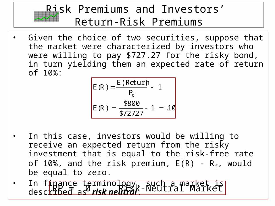
Risk Premiums and Investors’ Return-Risk Premiums
• Given the choice of two securities, suppose that the market were characterized by investors who were willing to pay $727.27 for the risky bond, in turn yielding them an expected rate of return of 10%:
• In this case, investors would be willing to receive an expected return from the risky investment that is equal to the risk-free rate of 10%, and the risk premium, E(R) - Rf, would be equal to zero.
• In finance terminology, such a market is described as risk neutral.
10.127.727$
800$)R(E
1P
)turn(ReE)R(E
0
RP = 0 → Risk-Neutral Market

Risk Premiums and Investors’ Return-Risk Premiums
• Instead of paying $727.27, suppose investors like the chance of obtaining returns greater than 10% (even though there is a chance of losing their investment), and as a result are willing to pay $750 for the risky bond. In this case, the expected return on the bond would be 6.67% and the risk premium would be negative:
• By definition, markets in which the risk premium is negative are called risk loving.
RP < 0 → Risk-Loving Market
033.10.0667.R)R(ERP
0667.1750$
800$)R(E
f

Risk Premiums and Investors’ Return-Risk Premiums
• Risk loving markets can be described as ones in which investors enjoy the excitement of the gamble and are willing to pay for it by accepting an expected return from the risky investment that is less than the risk-free rate.
• Even though there are some investors who are risk loving, a risk loving market is an aberration, with the exceptions being casinos, sports gambling markets, lotteries, and racetracks.

Risk Premiums and Investors’ Return-Risk Premiums
• Suppose most of the investors making up our market were unwilling to pay $727.27 or more for the risky bond.
• In this case, if the price of the risky bond were $727.27 and the price of the risk-free were $909.09, then there would be little demand for the risky bond and a high demand for the risk-free one.
• Holders of the risky bonds who wanted to sell would therefore have to lower their price, increasing the expected return. On the other hand, the high demand for the risk-free bond would tend to increase its price and lower its rate.

Risk Premiums and Investors’ Return-Risk Premiums
• Suppose the markets cleared when the price of the risky bond dropped to $701.75 to yield 14%, and the price of the risk-free bond increased to $917.43 to yield 9%:
• In this case, the risk premium would be 5%:
09.143.917$
000,1$R
14.175.701$
800$)R(E
f
05.09.14.R)R(ERP f

Risk Premiums and Investors’ Return-Risk Premiums
• By definition, markets in which the risk premium is positive are called risk-averse markets.
• In a risk-averse market, investors require compensation in the form of a positive risk premium to pay them for the risk they are assuming.
• Risk-averse investors view risk as a disutility, not a utility as risk-loving investors do.
RP > 0 → Risk-Averse Market

Risk Premiums and Investors’ Return-Risk Premiums
• Historically, security markets such as the stock and corporate bond markets have generated rates of return that, on average, have exceeded the rates on Treasury securities.
• This would suggest that such markets are risk averse.
• Since most markets are risk averse, a relevant question is the degree of risk aversion.
• The degree of risk aversion can be measured in terms of the size of the risk premium. The greater investors’ risk aversion, the greater the demand for risk-free securities and the lower the demand for risky ones, and thus the larger the risk premium.

Liquidity and Liquidity Premium
• Liquid securities are those that can be easily traded and in the short-run are absent of risk.
• In general, we can say that a less liquid bond will trade in the market at a price that yields a greater YTM than a more liquid one.

Liquidity and Liquidity Premium
• The difference in the YTM of a less liquid bond and the YTM of a more liquid one is defined as the liquidity premium, LP:
LP = YTM on Less Liquid Bond - YTM on More-Liquid Bond

Liquidity and Liquidity Premium
• Consider the equilibrium adjustment that would occur for two identical bonds that are priced with the same yields, but events occur that make one of the bonds less liquid.
• The decrease in liquidity on one of the bonds would cause its demand to decrease, shifting its bond demand curve to the left. The decrease in that bond’s liquidity would also make the other bond relatively more liquid, increasing its demand and shifting its demand curve to the right.
• Once the markets adjust to the liquidity difference between the bonds, then the less liquid bond’s price would be lower and its yield greater than the relative more liquid bond.
• Thus, the difference in liquidity between the bonds leads to a market adjustment in which there is a difference between rates due to their different liquidity features.

Liquidity Premium
SB
TBondforMarket
)(P )(i
SB
D1B
)(P )(i
T1i)Liquidity(
SB
C1i
)CinLiquidity(BD2
QuBond QuBond
C0i
T0i
D1B
D2B
D2B
CBondforMarket
D2B
D1B
D1B
The decrease in liquidity of Bond C decreases
its demand, shifting its bond demand curve to
the left.
Impact: A Higher Interest Rate on Bond C
The decrease in liquidity of Bond C increases the demand for Bond T, shifting its bond demand curve to the right.Impact: A Lower Interest Rate on Bond T

Taxability
• An investor in a 40% income tax bracket who purchased a fully-taxable 10% corporate bond at par, would earn an after-tax yield, ATY, of 6%: ATY = 10%(1-.4).
• In general, the ATY can be found by solving for that yield, ATY, that equates the bond’s price to the present value of its after-tax cash flows:
M
1tt
t0 )ATY1(
)ratetax1(CFP

Taxability and Pre-Tax Yield Spread
• Bonds that have different tax treatments but otherwise are identical will trade at different pre-tax YTM.
• That is, the investor in the 40% tax bracket would be indifferent between the 10% fully-taxable corporate bond and a 6% tax-exempt municipal bond selling at par, if the two bond were identical in all other respects.
• The two bonds would therefore trade at equivalent after-tax yields of 6%, but with a pre-tax yield spread of 4%:
%4%6%10iiSpreadYieldTaxePr M0
C0

Taxability and Pre-Tax Yield Spread
• In general, bonds whose cash flows are subject to less taxes trade at a lower YTM than bonds that are subject to more taxes.
• Historically, taxability explains why U.S. municipal bonds whose coupon interest is exempt from federal income taxes, have traded at yields below default-free U.S. Treasury securities even though many municipals are subject to default risk.

Term Structure of Interest Rates
• Term Structure examines the relationship between YTM and maturity, M.
• Yield Curve: Plot of YTM against M for bonds that are otherwise alike.

Term Structure of Interest Rates
• A yield curve can be constructed from current observations. For example, one could take all outstanding corporate bonds from a group in which the bonds are almost identical in all respects except their maturities, then generate the current yield curve.
• For investors who are more interested in long-run average yields instead of current ones, the yield curve could be generated by taking the average yields over a sample period (e.g., 5-year averages) and plotting these averages against their maturities.
• Finally, a widely-used approach is to generate a spot yield curve from spot rates.

Term Structure of Interest Rates
Shapes: Yield curves have tended to take on one of the three shapes:
1. They can be positively-sloped with long-term rates being greater than shorter-term ones.
• Such yield curves are called normal or upward sloping curves. They are usually convex from below, with the YTM flattening out at higher maturities.
2. Yield curves can also be negatively-sloped, with short-term rates greater than long-term ones.
• These curves are known as inverted or downward sloping yield curves. Like normal curves, these curves also tend to be convex, with the yields flattening out at the higher maturities.
3. Yield curves can be relatively flat, with YTM being invariant to maturity.

Term Structure of Interest Rates
Normal
Flat
Inverse
YTM
M

Theories of the Term Structure of Interest Rates
The actual shape of the yield curve depends on:• The types of bonds under consideration (e.g., AAA
bond versus B bond)
• Economic conditions (e.g., economic growth or recession, tight monetary conditions, etc.)
• The maturity preferences of investors and borrowers
• Investors' and borrowers' expectations about future rates, inflation, and the state of economy.

Theories of the Term Structure of Interest Rates
Four theories have evolved over the years to try to explain the shapes of yield curves:
1. Market Segmentation Theory (MST)
2. Preferred Habitat Theory (PHT)
3. Liquidity Premium Theory (LPT)
4. Pure Expectation Theory (PET)

Market Segmentation Theory
• MST: Yield curve is determined by supply and demand conditions unique to each maturity segment.
• MST assumes that markets are segmented by maturity.

Market Segmentation Theory
• Example: The yield curve for high quality corporate bonds could be segmented into two markets: – short-term – long-term

Market Segmentation Theory
Short-Term Market• The supply of short-term corporate bonds, such as
commercial paper would depend on business demand for short-term assets such as inventories, accounts receivables, and the like
• The demand for short-term corporate bonds would emanate from investors looking to invest their excess cash for short periods.
• The demand for short-term bonds by investors and the supply of such bonds by corporations would ultimately determine the rate on short-term corporate bonds.

Market Segmentation Theory
Long-Term Market• The supply of long-term bonds would come from
corporations trying to finance their long-term assets (plant expansion, equipment purchases, acquisitions, etc.).
• The demand for such bonds would come from investors, either directly or indirectly through institutions (e.g., pension funds, mutual funds, insurance companies, etc.), who have long-term liabilities and horizon dates.
• The demand for long-term bonds by investors and the supply of such bonds by corporations would ultimately determine the rate on long-term corporate bonds.

Market Segmentation Theory: Illustration
Short-Term Market
BondsST
.etc,sinventorie,receivableAccounts
:assetsTSofFinancing:Supply
dateshorizon
TSwithInvestors:Demand B
STr
Yield Curve for corporate bonds with two maturity segments: ST and LT

Market Segmentation Theory: Illustration
• Long-Term Market:
BondsLT
.etc,nsacquisitio,equipment,Plants
:assetsTLofFinancing:Supply
DateHorizonTL
withInvestors:Demand
BLTr

Market Segmentation Theory
• Important to MST is the idea of unique or independent markets.
• According to MST, the short‑term bond market is unaffected by rates determined in the intermediate or long‑term markets, and vice versa.
• This independence assumption is based on the premise that investors and borrowers have a strong need to match the maturities of their assets and liabilities.

MST: Supply and Demand Model• One way to examine how market forces determine the shape of
yield curves is to examine MST using our supply and demand analysis.
• Consider a simple world in which there are two types of corporate and government treasury bonds:
– Corporate bonds: long-term (BcLT) and short-term (Bc
ST)
– Treasury bonds: long-term (BTLT) and short-term (BT
LT).
• Assumptions: The supplies and demands for each sector and segment are based on the following assumptions:

MST: Supply and Demand Model
Assumption 1: Short-Term Bond Demand for Corporate and Treasury
• The most important factors determining the demand for short-term bonds (both corporate and Treasury) are the bond’s own price or interest rate, government policy, liquidity, and risk.
• Short-term bond demand is assumed to be inversely related to its price and directly related to its own rate (negatively sloped bond demand curves); government actions that affect the supply of loanable funds also can change bond demand (e.g., monetary policy changing bank reserve requirements).
• The demand for the short-term bond in one sector is also assumed to be an inverse function of the short-term rate in the other sector, but not the long-term rate in either its sector or the other sector given the assumption of segmented markets.

MST: Supply and Demand Model
• Assumption 1: Short-Term Bond Demand for Corporate and Treasury
)policygovernment,liquidity,risk,i,i(fBD
)policygovernment,liquidity,risk,i,i(fBD
cST
TST
TST
TST
cST
cST

MST: Supply and Demand Model
Assumption 2: Long-Term Bond Demand for Corporate and Treasury
• The most important factors determining the demand for long-term bonds (both corporate and Treasury) are the bond’s own price or interest rate, government policy such as monetary actions (e.g., change in bank reserve requirements), liquidity, and risk.
• Demand is assumed to be inversely related to its own price and directly related to its own rate (negatively sloped bond demand curves).
• In addition, the demand for the long-term bond in one sector is an inverse function of the long-term rate in the other sector, but not a function of short-term rates given the market segmentation assumption.

MST: Supply and Demand Model
• Assumption 2: Long-Term Bond Demand for Corporate and Treasury
)policygovernment,liquidity,risk,i,i(fBD
)policygovernment,liquidity,risk,i,i(fBD
cLT
TLT
TLT
TLT
cLT
cLT

MST: Supply and Demand Model
Assumption 3: Long-Term and Short-Term Bond Supplies for Corporate
• The supplies of short-term and long-term corporate bonds are directly related to their own prices and inversely to their own interest rates (positively sloped corporate bond supply curve) and directly related to general economic conditions, increasing in economic expansion and decreasing in recession.
)gdp,i(fBS
)gdp,i(fBS
cLT
cLT
cST
cST

MST: Supply and Demand Model
Assumption 4: Long-Term and Short-Term Bond Supplies for Treasury
• The supplies of Treasury bonds depend only on government actions (monetary and fiscal policy), and not on the economic state or interest rates.
• This assumption says that the sale or purchase of Treasury securities by the central bank or the Treasury is a policy decision. The assumption that the supply of Treasury securities depends on government actions and not interest rates means that the bond supply curve is vertical.
)policygovernment(fBS
)policygovernment(fBSTLT
TST

MST: Supply and Demand Model
• In the exhibit, the two equilibrium rates for short-term and long-term corporate bonds are plotted against their corresponding maturities to generate the yield curve for corporate bonds.
• Similarly, the equilibrium rates for short-term and long-term Treasury bonds are plotted against their corresponding maturities to generate the yield curve for Treasury bonds.
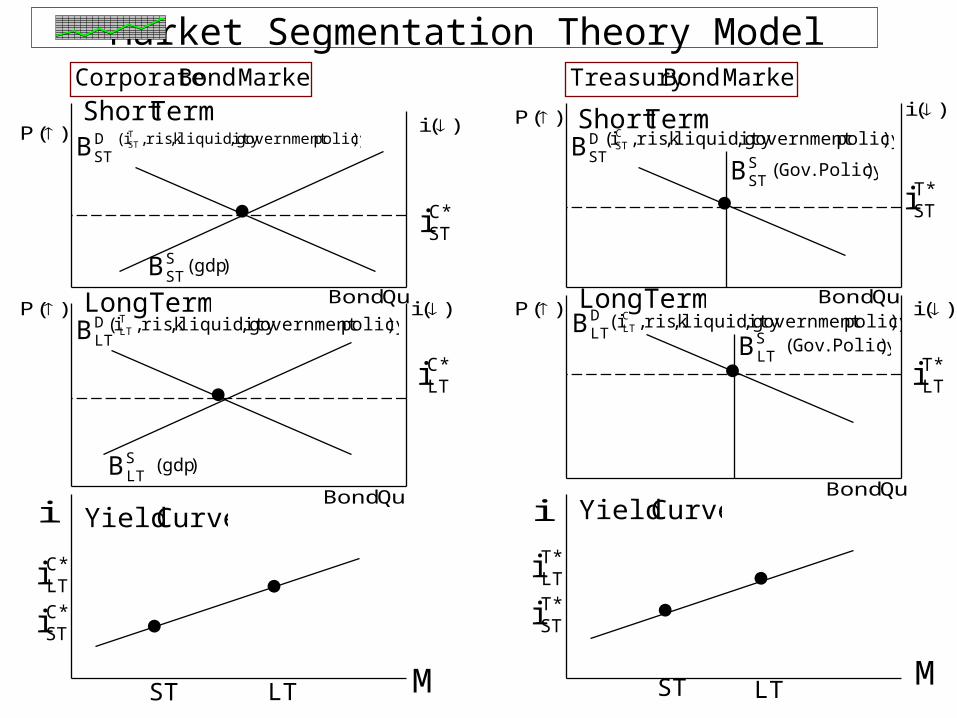
Market Segmentation Theory Model
)(P
SSTB
*CSTi
SSTB
M
TermShort
ST LT
CurveYield
MarketBondCorporate
)(i
MarketBondTreasury
TermLong)(P )(i
i
M
*CSTi
*CLTi
*CLTi
DSTB
SLTB
DLTB
TermShort)(P
)(P )(i
)(i
i
TermLong
CurveYield
SLTB
DLTB
DSTB
*TSTi
*TLTi
*TSTi
*TLTi
ST LT
)policygovernment,liquidity,risk,i( TST )policygovernment,liquidity,risk,i( C
ST
)policygovernment,liquidity,risk,i( TLT
)policygovernment,liquidity,risk,i( CLT
)gdp(
)gdp(
)Policy.Gov(
)Policy.Gov(
QuBond
QuBond QuBond
QuBond

MST: Supply and Demand Model
• These yield curves, in turn, capture an MST world in which interest rates for each segment are determined by the supply and demand for that bond, with the rates on bonds in the other maturity segments having no effect.
• In general, the positions and the shapes of the
yield curves depend on the factors that determine the supply and demand for short-term and long-term bonds.

MST: Cases Using S&D Model
Economic Expansion: • When an economy moves into a period of economic
growth, business demand for short-term and long-term assets increases.
• As a result, many companies issue more short-term bonds to finance their larger inventories and accounts receivables. They also issue more long-term bonds to finance their increase in investments in plants, equipment, and other long-term assets.
• In the bond market, these actions cause the short-term and the long-term supplies of bonds to increase as the economy grows.

MST: Cases Using S&D Model
Economic Expansion: • At the initial interest rates, the increase in bonds
outstanding creates an excess supply. This drives bond prices down and the YTM up.
• Using the supply and demand model, the economic expansion shifts the corporate short-term and long-term bond supply curves to the right, creating an excess supply for short-term bonds at ic*
ST and an excess supply for long-term bonds at ic*
LT.
• The excess causes corporate bond prices to fall and rates to rise until a new equilibrium is reached (ic**
ST and ic**
LT).

MST: Cases Using S&D Model
Economic Expansion: • As the rates on short-term and long-term corporate
bonds increase, short-term and long-term Treasury securities become relatively less attractive.
• As a result, the demands for short-term and long-term Treasuries decrease, shifting the short-term and long-term Treasury bond demand curves to the left and creating an excess supply in both Treasury markets at their initial rates.
• Like the corporate bond markets, the excess supply in the Treasury security markets will cause their prices to decrease and their rates to rise until a new equilibrium is attained.

MST: Cases Using S&D Model
Economic Expansion: • Thus, the supply and demand analysis shows that a
recession has a tendency to increase both short-term and long-term rates for corporate bonds, and by a substitution effect, increase short-term and long-term Treasury rates.
• Hence, an economic expansion causes the yield curves for both sectors to shift up.

Economic Expansion
)(P
SSTB
*CSTi
SSTB
M
TermShort
ST LT
CurveYield
MarketBondCorporate
)(i
MarketBondTreasury
TermLong)(P )(i
i
M*C
STi
*CLTi
**TLTi
DSTB
SLTB
DLTB
TermShort)(P
)(P )(i
)(i
i
TermLong
CurveYield
SLTBD
LTB
DSTB
*TSTi
*TLTi
*TSTi
ST LT
)gdp( **C
STiSSTB
)gdp( SSTB
*CLTi
**CSTi*C
LTi
)i(B CLT
DLT
)i(B CST
DST
**TSTi
**CLTi
*TLTi
**TSTi
**TLTi
QuBond
QuBond QuBond
QuBond

MST: Cases Using S&D Model
Government surplus in which the Treasury buys existing long-term Treasury bonds:
• When the Treasury uses a surplus to buy long-term Treasury securities there is a decrease in the supply of long-term Treasuries (leftward shift in the Treasury LT bond supply curve).
• The decrease in supply would push the price of the long-term government securities up, resulting in a lower long-term Treasury yield.

MST: Cases Using S&D Model
Government surplus in which the Treasury buys existing long-term Treasury bonds:
• In the corporate bond market, the lower rates on long-term government securities would lead to an increase in the demand for long-term corporate securities (rightward shift in the corporate LT bond demand curve), which, in turn, would lead to an excess demand in that market.
• As bondholders try to buy long-term corporate bonds, the prices on such bonds would increase, causing the yields on long-term corporate bonds to fall until a new equilibrium is reached.

MST: Cases Using S&D Model
Government surplus in which the Treasury buys existing long-term Treasury bonds:
• Thus, the purchase of the long-term Treasury securities decreases both long-term government and long-term corporate rates.
• Since the long-term market is assumed to be independent of short-term rates, the total adjustment to the Treasury’s purchase of long-term securities would occur through the decrease in long-term corporate and Treasury rates.
• If corporate and Treasury yield curves were initially flat, the Treasury’s action would cause the yield curves to become negatively sloped.

)(P SSTB
*CSTi
SSTB
M
TermShort
ST LT
CurveYield
MarketBondCorporate
)(i
MarketBondTreasury
TermLong)(P )(i
i
M
*CLTi
DSTB
SLTB
DLTB
TermShort)(P
)(P )(i
)(i
i
TermLong
CurveYield
SLTB
DLTB
DSTB
*TSTi
*TLTi
ST LT
*CLTi
*CLT
*CST ii
**CLTi
*TST
*TLT ii
**TLTi
**TLTi
Government surplus in which the Treasury buys existing long-term Treasury bonds
SLTB)i(B T
LTDLT
QuBond QuBond
QuBondQuBond

MST: Cases Using S&D Model
Contractionary open market operation in which the Central Bank sells some of it short-term Treasury securities:
• A contractionary OMO in which the Fed sells short-term Treasury securities would cause the price on short-term Treasury securities to decrease and their yield to increase. This would be reflected by a rightward shift in the short-term Treasury bond supply curve, as the Central Bank sells it securities to the public.
• As the yield on short-term Treasuries increases, the demand for short-term corporate would decrease (demand curve shifting left), leading to lower prices and higher yields on short-term corporate bonds.

MST: Cases Using S&D Model
Contractionary open market operation in which the Central Bank sells some of it short-term Treasury securities:
• Since the long-term market is assumed to be independent of short-term rates, the total adjustment to the Central bank’s sale of short-term securities to the public would be in the short-term corporate and Treasury markets with no impact on the long-term markets.
• If both the Treasury and corporate yield curves were initially flat, then the contractionary OMO would result in new negatively sloped yield curves.

)(P SSTB
*CSTi
SSTB
M
TermShort
ST LT
CurveYield
MarketBondCorporate
)(i
MarketBondTreasury
TermLong)(P )(i
i
M
**CSTi
DSTB
SLTBD
LTB
TermShort)(P
)(P )(i
)(i
i
TermLong
CurveYield
SLTB
DLTB
DSTB
*TSTi
*TLTi
ST LT
*CLTi
*CLT
*CST ii
**CSTi
*TST
*TLT ii
**TSTi
**TSTi
Contractionary Open Market Operation: Central Bank sells short-term Treasuries
SSTB
)i(B TST
DST
QuBond QuBond
QuBondQuBond
MST: Outline of Cases Using S&D Model
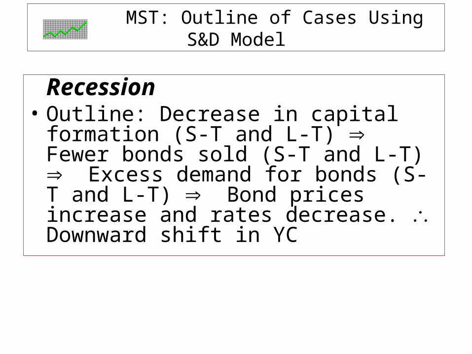
Recession• Outline: Decrease in capital formation (S-T
and L-T) Fewer bonds sold (S-T and L-T) Excess demand for bonds (S-T and L-T) Bond prices increase and rates decrease. Downward shift in YC

MST: Outline of Cases Using S&D Model
Expansionary open market operation in which the central bank buys short-term Treasury securities
• Outline: Central bank buys S-T Treasuries (T-bills) T-bill prices increase and rates decrease Substitution effect in which the demand for S-T corporate securities increase, causing their prices to increase and their yields to decrease. Tendency for YC to become positively sloped.

MST: Outline of Cases Using S&D Model
Treasury Sale of long-term Treasury bonds
• Outline: Treasury sells L-T Treasuries (T-Bonds) T-Bond prices decrease and yields increase Substitution effect in which the demand for L-T corporate securities decrease, causing their prices to decrease and their rates to increase. Tendency for YC to become positively sloped.

Preferred Habitat Theory (PHT)
• PHT assumes that investors and borrowers are willing to give up their desired maturity segment and assume market risk if rates are attractive.
• PHT asserts that investors and borrowers will be induced to forego their perfect hedges and shift out of their preferred maturity segments when supply and demand conditions in different maturity markets do not match.

Preferred Habitat Theory (PHT)
• PHT is a necessary extension of the MST: – If an economy is poorly hedged (e.g., more
investors want ST investments and more borrowers want to borrow LT), then the market will not be in equilibrium.
– In such cases, ST and LT rates will change and the markets will clear as investors and borrowers give up their hedge.

Preferred Habitat Theory (PHT)
• To illustrate PHT, consider an economic world in which, on the demand side, investors in corporate securities, on average, prefer short-term to long-term instruments, while on the supply side, corporations have a greater need to finance long-term assets than short-term, and therefore prefer to issue more long-term bonds than short-term.
• Combined, these relative preferences would cause an excess demand for short-term bonds and an excess supply for long-term claims and an equilibrium adjustment would have to occur.

Preferred Habitat Theory (PHT)
• In the long-term market, the excess supply would force issuers to lower their bond prices, thus increasing bond yields and inducing some investors to change their short-term investment demands.
• In the short-term market, the excess demand would cause bond prices to increase and rates to fall, inducing some corporations to finance their long-term assets by selling short-term claims.
• Ultimately, equilibriums in both markets would be reached with long-term rates higher than short-term rates, a premium necessary to compensate investors and borrowers/issuers for the market risk they've assumed.

Preferred Habitat Theory
• Poorly Hedged Economy: Investors, on average, prefer ST investments; corporate borrowers, on average, prefer to borrow LT (sell LT corporate bonds):
STprefer
Investors
LTprefer
Borrower
STinDemandExcess
LTinSupplyExcess
STB
ST r,P
LTBLT r,P
BorrowersLT
attractsrST
InvestorsST
attractsrLT

Liquidity Preference Theory
• Long-term bonds are more price sensitive to interest rate changes than short-term bonds. As a result, the prices of long-term securities tend to be more volatile and therefore more risky than short-term securities.
• The Liquidity Premium Theory (LPT), also referred to as the Risk Premium Theory (RPT), posits that there is a liquidity premium for long-term bonds over short-term bonds.

Liquidity Preference Theory
• According to LPT, if investors were risk averse, then they would require some additional return (liquidity premium, LP) in order to hold long-term bonds instead of short-term ones.
0rrLP STLT

Liquidity Preference Theory
• Thus, if the yield curve were initially flat, but had no risk premium factored in to compensate investors for the additional volatility they assumed from buying long-term bonds, then the demand for long-term bonds would decrease and their rates increase until risk-averse investors were compensated.
• In this case, the yield curve would become positively sloped.

Pure Expectations Theory
• Expectation theories address the question of what impact expectations have on the current yield curve.
• One of these theories is the Pure Expectations Theory (PET); also referred to as the unbiased expectations theory (UET).
• PET posits that the yield curve is governed by the condition that the implied forward rate is equal to the expected sport rate.

Pure Expectations Theory
To illustrate PET:• Consider a market consisting of only two bonds: a risk-free
one‑year zero-coupon bond and a risk-free two‑year zero-coupon bond, both with principals of $100.
• Suppose that supply and demand conditions are such that both the one‑year and two‑year bonds are trading at an 8% YTM.
• Suppose that the market expects the yield curve to shift up to 10% next year, but, as yet, has not factored that expectation into its current investment decisions.
• Finally, assume the market is risk-neutral, such that investors do not require a risk premium for investing in risky securities (i.e., they will accept an expected rate on a risky investment that is equal to the risk-free rate).

Pure Expectations Theory
Question:• What is the impact of the expectation
on the current yield curve?

Pure Expectations Theory
• Consider investors with HD = 2 years• Alternatives:
– Buy 2-year bond at 8%– Buy a series of 1-year bonds: 1-year bond today at 8%
and 1-year bond one year later at E(r11) = 10%. The expected return from the series would be 9%:
• In a risk-neutral world, investors with HD = 2 years would prefer the series of 1-year bonds over the 2-year bond.
09.1)10.1)(08.1(YTM 2/1Series:2

Pure Expectations Theory
• Consider investors with HD = 1 year.• Alternatives:
– Buy 1-year bond at 8%.– Buy a 2-year bonds at 8% for P2 = 100/(1.08)2 =
85.734, then sell it one year later at an expected price of E(P11) = 100/(1.10) = 90.91. The expected rate of return would be 6%:
• In a risk-neutral world, investors with HD = 1 year would prefer the 1-year bond over the 2-year bond.
06.734.85
734.8591.90)r(E 11

Pure Expectations Theory
• Thus, in a risk-neutral market with an expectation of higher rates next year, both investors with one‑year horizon dates and investors with two‑year horizon dates would purchase one‑year instead of two-year bonds
• If enough investors do this, an increase in the demand for one‑year bonds and a decrease in the demand for two‑year bonds would occur until the average annual rate on the two‑year bond is equal to the equivalent annual rate from the series of one‑year investments (or the one‑year bond's rate is equal to the rate expected on the two‑year bond held one year).

Pure Expectations Theory
• Investors with HD of 2 years and those with HD of 1 year would prefer one-year bonds over two- year bonds.
• Market Response: 2
B2
D2 rPB 1
B1
D1 rPB
M
r
10%
8%
yr1 yr2
PETSlopedPositively
becomesYC

Pure Expectations Theory
• In the example, if the price on a two-year bond fell such that it traded at a YTM of 9% and the rate on a one-year bond stayed at 8%, then investors with two-year horizon dates would be indifferent between a two-year bond yielding a certain 9% and a series of one-year bonds yielding 10% and 8%, for an expected rate of 9%.
• Investors with one-year horizon dates would likewise be indifferent between a one-year bond yielding 8% and a two-year bond purchased at 9% and sold one year later at 10%, for an expected one-year rate of 8%.

Pure Expectations Theory
• Thus in this case, the impact of the market's expectation of higher rates would be to push 2-year rates up to 9%.
• Note: With YTM2 = 9% and YTM1 = 8%, the implied forward rate is f11 = 10% -- the same rate as the expected rate E(r11).

Pure Expectations Theory
• Assume that the market response is one in which only the demand for 2-year bonds is affected by the expectations.
09.rruntilr
rPB
Series:222
2B2
D2
M
r
%10
%8
yr1 yr2
PET%9
)r(Efthen,holdsPETif,Thus
).r(E%10fthen
,%8YTM%,9YTMWhen:Note
MtMt
1111
12

Pure Expectations Theory
• In the above example, the yield curve is positively sloped, reflecting expectations of higher rates.
• By contrast, if the yield curve were currently flat at 10% and there was a market expectation that it would shift down to 8% next year, then the expectation of lower rates would cause the yield curve to become negatively sloped.

Pure Expectations Theory
• That is, given a yield curve currently flat at 10% and a market expectation that it would shift down to 8% next year, an investor with a two-year horizon date would prefer the two-year bond at 10% to a series of one-year bonds yielding an expected rate of only 9% (E(R) = [(1.10)(1.08)]1/2 -1 = .09).
• Similarly, an investor with a one-year horizon would also prefer buying a two-year bond that has an expected rate of return of 12% (P2 =100/(1.10)2 = 82.6446, E(P11) = 100/1.08 = 92.5926, E(R) = [92.5926-82.6446]/82.6446 = .12) to the one-year bond that yields only 10%.

Pure Expectations Theory
• In markets for both one-year and two-year bonds, the expectations of lower rates would cause the demand and price of the two-year bond to increase, lowering its rate, and the demand and price for the one-year bond to decrease, increasing its rate.

Pure Expectations Theory
2B2
D2 rPB
:sponseReMarket
M
r
%10
%8
yr1 yr2
PET
Market expects the yield curve to shift down from 10% to 8%.
Investors with two-year horizon dates would prefer the two-year bond at 10% to a series of one-year bonds yielding an expected rate of only 9%: (E(R) = [(1.10)(1.08)]1/2 -1 = .09)
Investor with a one-year horizon would prefer buying a two-year bond that has an expected rate of return of 12% to the one-year bond that yields only 10%:P2 =100/(1.10)2 = 82.6446 E(P11) = 100/1.08 = 92.5926 E(R) = [92.5926-82.6446]/82.6446 = .12
1B
1D1 rPB
:sponseReMarket
YC become negatively sloped

Pure Expectations Theory
• The adjustments would continue until the rate on the two-year bond equaled the average rate from the series of one-year investments, or until the rate on the one-year bond equaled the expected rate from holding a two-year bond one year (or when the implied forward rate is equal to expected spot rates).
• In this case, if one-year rates stayed at 8%, then the demand for the two-year bond would increase until it was priced to yield 9% - the expected rate from the series: [(1.10)(1.08)]1/2 -1 = .09

Pure Expectations Theory
• Assume that the market response is one in which only the demand for 2-year bonds is affected by the expectations.
09.rruntilr
rPB
Series:222
2B2
D2
M
r
%10
%8
yr1 yr2
PET
%9

Features of PET
1. One of the features of the PET is that in equilibrium the yield curve reflects current expectations about future rates. From our preceding examples:• When the equilibrium yield curve was
positively sloped, the market expected higher rates in the future
• When the curve was negatively sloped, the market expected lower rates.

Features of PET2. PET intuitively captures what should be considered as
normal market behavior. – For example, if long-term rates were expected to be higher
in the future, long-term investors would not want to purchase long-term bonds now, given that next period they would be expecting higher yields and lower prices on such bonds. Instead, such investors would invest in short-term securities now, reinvesting later at the expected higher long-term rates.
– In contrast, borrowers/issuers wishing to borrow long-term would want to sell long-term bonds now instead of later at possibly higher rates.
– Combined, the decrease in demand for long-term bonds by investors and the increase in the supply of long-term bonds by borrowers would serve to lower long-term bond prices and increase yields, leading to a positively-sloped yield curve.

Features of PET
3. If PET strictly holds (i.e., we can accept all of the model's assumptions), then the expected future rates would be equal to the implied forward rates. As a result, one could forecast futures rates and future yield curves by simply calculating implied forward rates from current rates.

Features of PET
• The last feature suggests that given a spot yield curve, one could use PET to estimate next period's spot yield curve by determining the implied forward rates.
• The exhibit on the next slide shows spot rates on bonds with maturities ranging from one year to five years (Column 2). From these rates, expected spot rates (St) are generated for bonds one year from the present (Column 3) and two years from the present (Column 4). The expected spot rates shown are equal to their corresponding implied forward rates.

Features of PET
(1) (2) (3) (4)
Maturity Spot Rates Expected Spot Rates One year from Present
Expected Spot Rates Two Years
from Present
1
2
3
4
5
10.0%
10.5%
11.0%
11.5%
12.0%
f11 = 11.0%
f21 = 11.5%
f31 = 12.0%
f41 = 12.5%
f12 = 12.0%
f22 = 12.5%
f32 = 13.0%

Features of PET
12.1)105.1(
)11.1(f
1)S1(
)S1(f
1)]f1()S1[(S
1)]f1)(f1)(S1[(S
f
2
3
12
22
33
12
3/112
223
3/1121113
12
13.1)105.1(
)12.1(f
1)S1(
)S1(f
1])f1()S1[(S
1)]f1)(f1)(f1)(f1)(S1[(S
f
3/1
2
5
32
3/1
22
55
32
5/1332
225
5/11413121115
32
1)S1(
)S1(f
:FormulaGeneralM/1
tt
tMtM
Mt

Features of PET
• According to PET, if the market is risk-neutral, then the implied forward rate is equal to the expected spot rate, and in equilibrium, the expected rate of return for holding any bond for one year would be equal to the current spot rate on one-year bonds.

Features of PET• For example, the expected rate of return from purchasing a
two-year zero-coupon bond at the spot rate of 10.5% and selling it one year later at an expected one-year spot rate equal to the implied forward rate of f11 = 11% is 10%. This is the same rate obtained from investing in a one-year bond:
8984.81)105.1(
100P
09.9011.1
100)P(E
10.8984.81
8984.8109.90)R(E
220
11

Features of PET
• Similarly, the expected rate of return from holding a three-year bond for one year, then selling it at the implied forward rate of f21 is also 10%. That is:
• Any of the bonds with spot rates shown in the exhibit would have expected rates for one year of 10% if the implied forward rate were used as the estimated expected rate.
1191.73)11.1(
100P
43596.80)115.1(
100)P(E
10.1191.73
1191.7343596.80)R(E
330
221
Features of PET
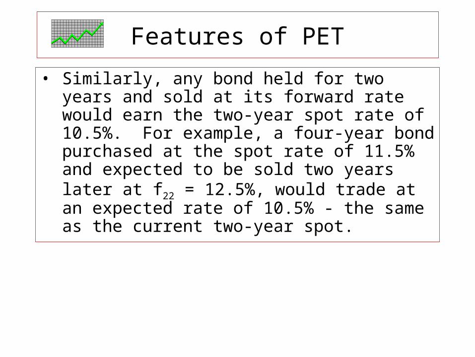
• Similarly, any bond held for two years and sold at its forward rate would earn the two-year spot rate of 10.5%. For example, a four-year bond purchased at the spot rate of 11.5% and expected to be sold two years later at f22 = 12.5%, would trade at an expected rate of 10.5% - the same as the current two-year spot.

Features of PET
• Analysts often refer to forward rates as hedgable rates.
• The most practical use of forward rates or expected spot yield curves generated from forward rates is that they provide cut-off rates, useful in evaluating investment decisions.
• For example, an investor with a one-year horizon date should only consider investing in the two-year bond in our above example, if she expected one-year rates one year later to be less than f11 = 11%; that is, assuming she is risk-averse and wants an expected rate greater than 10%.
• Thus, forward rates serve as a good cut-off rate for evaluating investments.

Websites
• Historical interest rate data on different bonds can be found at the Federal Reserve site www.federalreserve.gov/releases/h15/data.htm
and www.research.stlouisfed.org/fred2
• For information on Federal Reserve policies go to
www.federalreserve.gov/policy.htm
• For information on European Central Banks go to
www.ecb.int

Websites
• Current and historical data on U.S. government expenditures and revenues can be found at www.gpo.gov/usbudget.
• Yield curves can be found at a number of sites:www.ratecurve.com and www.bloomberg.com