Chapter 3 The basic OLG model: Diamondweb.econ.ku.dk/okocg/MAT-OEK/MakØk2/MakØk2-2016...68 CHAPTER 3. THE BASIC OLG MODEL: DIAMOND The model takes elementary forms of heterogeneity

Chapter 3

The basic OLG model: Diamond

There exists two main analytical frameworks for analyzing the basic intertem-poral choice, consumption versus saving, and the dynamic implications of thischoice: overlapping-generations (OLG) models and representative agent models.In the first type of models the focus is on (a) the interaction between differentgenerations alive at the same time, and (b) the never-ending entrance of newgenerations and thereby new decision makers. In the second type of models thehousehold sector is modelled as consisting of a finite number of infinitely-liveddynasties. One interpretation is that the parents take the utility of their descen-dants into account by leaving bequests and so on forward through a chain ofintergenerational links. This approach, which is also called the Ramsey approach(after the British mathematician and economist Frank Ramsey, 1903-1930), willbe described in Chapter 8 (discrete time) and Chapter 10 (continuous time).In the present chapter we introduce the OLG approach which has shown its

usefulness for analysis of many issues such as: public debt, taxation of capitalincome, financing of social security (pensions), design of educational systems,non-neutrality of money, and the possibility of speculative bubbles. We will focuson what is known as Diamond’s OLG model1 after the American economist andNobel Prize laureate Peter A. Diamond (1940-).Among the strengths of the model are:

• The life-cycle aspect of human behavior is taken into account. Although theeconomy is infinitely-lived, the individual agents are not. During lifetimeone’s educational level, working capacity, income, and needs change andthis is reflected in the individual labor supply and saving behavior. Theaggregate implications of the life-cycle behavior of coexisting individualagents at different stages in their life is at the centre of attention.

1Diamond (1965).

67

68 CHAPTER 3. THE BASIC OLG MODEL: DIAMOND

• The model takes elementary forms of heterogeneity in the population intoaccount − there are “old”and “young”, there are the currently-alive peo-ple and the future generations whose preferences are not reflected in currentmarket transactions. Questions relating to the distribution of income andwealth across generations can be studied. For example, how does the invest-ment in fixed capital and environmental protection by current generationsaffect the conditions for the succeeding generations?

3.1 Motives for saving

Before going into the specifics of Diamond’s model, let us briefly consider whatmay in general motivate people to save:

(a) The consumption-smoothing motive for saving. Individuals go through a lifecycle where earnings typically have a hump-shaped time pattern; by savingand dissaving the individual then attempts to obtain the desired smoothingof consumption across lifetime. This is the essence of the life-cycle savinghypothesis put forward by Nobel laureate Franco Modigliani (1918-2003)and associates in the 1950s. This hypothesis states that consumers plantheir saving and dissaving in accordance with anticipated variations in in-come and needs over lifetime. Because needs vary less over lifetime thanincome, the time profile of saving tends to be hump-shaped with some dis-saving early in life (for instance if studying), positive saving during theyears of peak earnings and then dissaving after retirement.

(b) The precautionary motive for saving. Income as well as needs may varydue to conditions of uncertainty: sudden unemployment, illness, or otherkinds of bad luck. By saving, the individual can obtain a buffer againstsuch unwelcome events.

Horioka and Watanabe (1997) find that empirically, the saving motives (a)and (b) are of dominant importance (Japanese data). Yet other motives include:

(c) Saving enables the purchase of durable consumption goods and owner-occupiedhousing as well as repayment of debt.

(d) Saving may be motivated by the desire to leave bequests to heirs.

(e) Saving may simply be motivated by the fact that financial wealth may leadto social prestige and economic or political power.

c© Groth, Lecture notes in macroeconomics, (mimeo) 2016.

3.2. The model framework 69

Diamond’s OLG model aims at simplicity and concentrates on motive (a). Infact only one aspect of motive (a) is considered, namely the saving for retirement.People live for two periods only, as “young”they work full-time and as “old”theyretire and live by their savings. The model abstracts from a possible bequestmotive.Now to the details.

3.2 The model framework

The flow of time is divided into successive periods of equal length, taken as thetime unit. Given the two-period lifetime of (adult) individuals, the period lengthis understood to be very long, around, say, 30 years. The main assumptions are:

1. The number of young people in period t, denoted Lt, changes over timeaccording to Lt = L0(1 + n)t, t = 0, 1, 2, ..., where n is a constant, n > −1.Indivisibility is ignored and so Lt is just considered a positive real number.

2. Only the young work. Each young supplies one unit of labor inelastically.The division of available time between work and leisure is thereby consideredas exogenous.

3. Output is homogeneous and can be used for consumption as well as invest-ment in physical capital. Physical capital is the only non-human asset inthe economy; it is owned by the old and rented out to the firms. Output isthe numeraire (unit of account) used in trading. Money (means of payment)is ignored.2

4. The economy is closed (no foreign trade).

5. Firms’technology has constant returns to scale.

6. In each period three markets are open, a market for output, a market forlabor services, and a market for capital services. Perfect competition rulesin all markets. Uncertainty is absent; when a decision is made, its conse-quences are known.

7. Agents have perfect foresight.

Assumption 7 entails the following. First, the agents are assumed to have“rational expectations”or, with a better name, “model-consistent expectations”.

2As to the disregard of money we may imagine that agents have safe electronic accounts ina fictional central bank allowing costless transfers between accounts.



This means that forecasts made by the agents coincide with the forecasts thatcan be calculated on the basis of the model. Second, as there are no stochasticelements in the model (no uncertainty), the forecasts are point estimates ratherthan probabilistic forecasts. Thereby the model-consistent expectations take theextreme form of perfect foresight : the agents agree in their expectations about thefuture evolution of the economy and ex post this future evolution fully coincideswith what was expected.

Figure 3.1: The two-period model’s time structure.

Of course, this is an unrealistic assumption. The motivation is to simplify ina first approach. The results that emerge will be the outcome of economic mech-anisms in isolation from expectational errors. In this sense the model constitutesa “pure”case (benchmark case).The time structure of the model is illustrated in Fig. 3.1. In every period

two generations are alive and interact with each other as indicated by the arrows.The young supply labor and earn a labor income. They consume an endogenousfraction of this income and save the remainder for retirement. Thereby the youngoffset the dissaving by the old, and possibly positive net investment arises in theeconomy. At the end of the first period the savings by the young are convertedinto direct ownership of capital goods. In the next period the now old owners ofthe capital goods rent them out to the firms. We may imagine that the firms areowned by the old, but this ownership is not visible in the equilibrium allocationbecause pure profits will be nil due to the combination of perfect competition andconstant returns to scale.Let the output good be the numeraire and let rt denote the rental rate for

capital in period t; that is, rt is the real price a firm has to pay at the end of


3.2. The model framework 71

period t for the right to use one unit of someone else’s physical capital throughperiod t. So the owner of Kt units of physical capital receives a

real (net) rate of return on capital =rtKt − δKt

Kt

= rt − δ, (3.1)

where δ is the rate of physical capital depreciation which is assumed constant,0 ≤ δ ≤ 1.Suppose there is also a market for loans. Assume you have lent out one unit

of output from the end of period t− 1 to the end of period t. If the real interestrate in the loan market is rt, then, at the end of period t you should get back1 + rt units of output. In the absence of uncertainty, equilibrium requires thatcapital and loans give the same rate of return,

rt − δ = rt. (3.2)

This no-arbitrage condition indicates how the rental rate for capital and the moreeveryday concept, the interest rate, would be related in an equilibrium whereboth the market for capital services and a loan market were active. We shallsee, however, that in this model no loan market will be active in an equilibrium.Nevertheless we will follow the tradition and call the right-hand side of (3.2) theinterest rate.Table 3.1 provides an overview of the notation. As to our timing convention,

notice that any stock variable dated t indicates the amount held at the beginningof period t. That is, the capital stock accumulated by the end of period t − 1and available for production in period t is denoted Kt. We therefore write Kt

= (1 − δ)Kt−1 + It−1 and Yt = F (Kt, Lt), where F is an aggregate productionfunction. In this context it is useful to think of “period t”as running from datet to right before date t + 1. So period t is the half-open time interval [t, t+ 1)on the continuous-time axis. Whereas production and consumption take placein period t, we imagine that all decisions are made at discrete points in timet = 0, 1, 2, ... (“dates”). We further imagine that receipts for work and lending aswell as payment for the consumption in period t occur at the end of the period.These timing conventions are common in discrete-time growth and business cycletheory;3 they are convenient because they make switching between discrete andcontinuous time analysis fairly easy.

3In contrast, in the accounting and finance literature, typically Kt would denote the end-of-period-t stock that begins to yield its services next period.



Table 3.1. List of main variable symbolsSymbol MeaningLt the number of young people in period tn generation growth rateKt aggregate capital available in period tc1t consumption as young in period tc2t consumption as old in period twt real wage in period trt real interest rate (from end of per. t− 1 to end of per. t)ρ rate of time preference (impatience)θ elasticity of marginal utilityst saving of each young in period tYt aggregate output in period t

Ct = c1tLt + c2tLt−1 aggregate consumption in period tSt = Yt − Ct aggregate gross saving in period tδ ∈ [0, 1] capital depreciation rate

Kt+1 −Kt = It − δKt aggregate net investment in period t

3.3 The saving by the young

Suppose the preferences of the young can be represented by a lifetime utilityfunction as specified in (3.3). Given wt and rt+1, the decision problem of theyoung in period t then is:

maxc1t,c2t+1

U(c1t, c2t+1) = u(c1t) + (1 + ρ)−1u(c2t+1) s.t. (3.3)

c1t + st = wt · 1 (wt > 0), (3.4)

c2t+1 = (1 + rt+1)st (rt+1 > −1), (3.5)

c1t ≥ 0, c2t+1 ≥ 0. (3.6)

The interpretation of the variables is given in Table 3.1 above. We may thinkof the “young”as a household consisting of one adult and 1 + n children whoseconsumption is included in c1t. Note that “utility”appears at two levels. Thereis a lifetime utility function, U, and a period utility function, u.4 The latter isassumed to be the same in both periods of life (this has no effects on the qualita-tive results and simplifies the exposition). The period utility function is assumedtwice continuously differentiable with u′ > 0 and u′′ < 0 (positive, but diminish-ing marginal utility of consumption). Many popular specifications of u, e.g., u(c)= ln c, have the property that limc→0 u(c) = −∞; then we define u(0) = −∞.

4Other names for these two functions are the intertemporal utility function and the subutilityfunction, respectively.


3.3. The saving by the young 73

The parameter ρ is called the rate of time preference. It acts as a utilitydiscount rate, whereas (1+ρ)−1 is a utility discount factor. By definition, ρ > −1,but ρ > 0 is usually assumed. We interpret ρ as reflecting the degree of impatiencewith respect to the “arrival”of utility. When preferences can be represented inthis additive way, they are called time-separable. In principle, as seen from periodt the interest rate appearing in (3.5) should be interpreted as an expected realinterest rate. But as long as we assume perfect foresight, there is no need thatour notation distinguishes between actual and expected magnitudes.

Box 3.1. Discount rates and discount factors

By a discount rate is meant an interest rate applied in the construction of a dis-count factor. A discount factor is a factor by which future benefits or costs, mea-sured in some unit of account, are converted into present equivalents. The higherthe discount rate the lower the discount factor.

One should bear in mind that a discount rate depends on what is to be dis-counted. In (3.3) the unit of account is “utility”and ρ acts as a utility discount rate.In (3.7) the unit of account is the consumption good and rt+1 acts as a consump-tion discount rate. If people also work as old, the right-hand side of (3.7) wouldread wt + (1 + rt+1)−1wt+1 and thus rt+1 would act as an earnings discount rate.This will be the same as the consumption discount rate if we think of real incomemeasured in consumption units. But if we think of nominal income, that is, incomemeasured in monetary units, there would be a nominal earnings discount rate,namely the nominal interest rate, which in an economy with inflation will exceedthe consumption discount rate. Unfortunately, confusion of different discount ratesis not rare.

In (3.5) the interest rate rt+1 acts as a (net) rate of return on saving.5 Aninterest rate may also be seen as a discount rate relating to consumption over time.Indeed, by isolating st in (3.5) and substituting into (3.4), we may consolidatethe two period budget constraints of the individual into one budget constraint,

c1t +1

1 + rt+1

c2t+1 = wt. (3.7)

5While st in (3.4) appears as a flow (non-consumed income), in (3.5) st appears as a stock(the accumulated financial wealth at the end of period t). This notation is legitimate becausethe magnitude of the two is the same when the time unit is the same as the period length.Indeed, the interpretation of st in (3.5) st = st ·∆t = st · 1 units of account.In real life the gross payoff of individual saving may sometimes be nil (if invested in a project

that completely failed). Unless otherwise indicated, it is in this book understood that an interestrate is a number exceeding −1 as indicated in (3.5). Thereby the discount factor 1/(1 + rt+1)is well-defined. In general equilibrium, the condition 1 + rt+1 > 0 is always met in the presentmodel.



In this intertemporal budget constraint the interest rate appears as the discountrate entering the discount factor converting future amounts of consumption intopresent equivalents, cf. Box 3.1.

Solving the saving problem

To avoid the possibility of corner solutions, we impose the No Fast Assumption

limc→0

u′(c) =∞. (A1)

In view of the sizeable period length in the model, this is definitely plausible.Inserting the two budget constraints into the objective function in (3.3), we get

U(c1t, c2t+1) = u(wt−st) +(1+ρ)−1u((1+rt+1)st) ≡ Ut(st), a function of only onedecision variable, st. According to the non-negativity constraint on consumptionin both periods, (3.6), st must satisfy 0 ≤ st ≤ wt. Maximizing with respect tost gives the first-order condition

dUtdst

= −u′(wt − st) + (1 + ρ)−1u′((1 + rt+1)st)(1 + rt+1) = 0. (FOC)

The second derivative of Ut is

d2Utds2

t

= u′′(wt − st) + (1 + ρ)−1u′′((1 + rt+1)st)(1 + rt+1)2 < 0. (SOC)

Hence there can at most be one st satisfying (FOC). Moreover, for a positivewage income there always exists such an st. Indeed:

LEMMA 1 Let wt > 0 and suppose the No Fast Assumption (A1) applies. Thenthe saving problem of the young has a unique solution st = s(wt, rt+1). Thesolution is interior, i.e., 0 < st < wt, and st satisfies (FOC).

Proof. Assume (A1). For any s ∈ (0, wt), dUt(s)/ds > −∞. Now consider theendpoints s = 0 and s = wt. By (FOC) and (A1),

lims→0

dUtds

= −u′(wt) + (1 + ρ)−1(1 + rt+1) lims→0

u′((1 + rt+1)s) =∞,

lims→w

dUtds

= − lims→wt

u′(wt − s) + (1 + ρ)−1(1 + rt+1)u′((1 + rt+1)wt) = −∞.

By continuity of dUt/ds follows that there exists an st ∈ (0, wt) such that ats = st, dUt/ds = 0. This is an application of the intermediate value theorem. Itfollows that (FOC) holds for this st. By (SOC), st is unique and can therefore



be written as an implicit function, s(wt, rt+1), of the exogenous variables in theproblem, wt and rt+1. �Inserting the solution for st into the two period budget constraints, (3.4) and

(3.5), we immediately get the optimal consumption levels, c1t and c2t+1.The simple optimization method we have used here is called the substitution

method : by substitution of the constraints into the objective function an uncon-strained maximization problem is obtained.6

The consumption Euler equation

The first-order condition (FOC) can conveniently be written

u′(c1t) = (1 + ρ)−1u′(c2t+1)(1 + rt+1). (3.8)

This is known as an Euler equation, after the Swiss mathematician L. Euler (1707-1783) who was the first to study dynamic optimization problems. In the presentcontext the condition is called a consumption Euler equation.Intuitively, in an optimal plan the marginal utility cost of saving must equal

the marginal utility benefit obtained by saving. The marginal utility cost ofsaving is the opportunity cost (in terms of current utility) of saving one moreunit of account in the current period (approximately). This one unit of accountis transferred to the next period with interest so as to result in 1 + rt+1 units ofaccount in that period. An optimal plan requires that the utility cost equals theutility benefit of instead having 1 + rt+1 units of account in the next period. Andthis utility benefit is the discounted value of the extra utility that can be obtainednext period through the increase in consumption by 1+rt+1 units compared withthe situation without the saving of the marginal unit.It may seem odd to attempt an intuitive interpretation this way, that is, in

terms of “utility units”. The utility concept is just a convenient mathematical de-vice used to represent the assumed preferences. Our interpretation is only meantas an as-if interpretation: as if utility were something concrete. An interpretationin terms of concrete measurable quantities goes like this. We rewrite (3.8) as

u′(c1t)

(1 + ρ)−1u′(c2t+1)= 1 + rt+1. (3.9)

The left-hand side measures the marginal rate of substitution, MRS, of consump-tion as old for consumption as young, evaluated at the point (c1, c2). MRS isdefined as the increase in period-t + 1 consumption needed to compensate for a

6Alternatively, one could use the Lagrange method.



marginal decrease in period-t consumption. That is,

MRSc2c1 = −dc2t+1

dc1t

|U=U =u′(c1t)

(1 + ρ)−1u′(c2t+1), (3.10)

where we have used implicit differentiation in U(c1t, c2t+1) = U . The right-handside of (3.9) indicates the marginal rate of transformation, MRT, which is therate at which saving allows an agent to shift consumption from period t to periodt+ 1 via the market. In an optimal plan MRS must equal MRT.Even though interpretations in terms of “MRS equals MRT”are more satis-

factory, we will often use “as if” interpretations like the one before. They are aconvenient short-hand for the more elaborate interpretation.By the Euler equation (3.8),

ρ Q rt+1 implies u′(c1t) R u′(c2t+1), i.e., c1t Q c2t+1,

respectively, in the optimal plan (because u′′ < 0). That is, absent uncertaintythe optimal plan entails either increasing, constant or decreasing consumptionover time according to whether the rate of time preference is below, equal to, orabove the market interest rate, respectively. For example, when ρ < rt+1, theplan is to start with relatively low consumption in order to take advantage of therelatively high rate of return on saving.Note that there are infinitely many pairs (c1t, c2t+1) satisfying the Euler equa-

tion (3.8). Only when requiring the two period budget constraints, (3.4) and(3.5), satisfied, do we get the unique solution st and thereby the unique solutionfor c1t and c2t+1.

Properties of the saving function

The first-order condition (FOC), where the two budget constraints are inserted,determines the saving as an implicit function of the market prices faced by theyoung decision maker, i.e., st = s(wt, rt+1).The partial derivatives of this function can be found by applying the implicit

function theorem on (FOC). A practical procedure is the following. We firstinterpret dUt/dst in (FOC) as a function, f, of the variables involved, st, wt, andrt+1, i.e.,

dUtdst

= −u′(wt − st) + (1 + ρ)−1u′((1 + rt+1)st)(1 + rt+1) ≡ f(st, wt, rt+1).

By (FOC),f(st, wt, rt+1) = 0. (*)



The implicit function theorem (see Math tools) now implies that if ∂f/∂st 6= 0,then the equation (*) defines st as an implicit function of wt and rt+1, st =s(wt, rt+1), with partial derivatives

∂st∂wt

= −∂f/∂wtD

and∂st∂rt+1

= −∂f/∂rt+1

D,

where D ≡ ∂f/∂st ≡ d2Ut/ds2t < 0 by (SOC). We find

∂f

∂wt= −u′′(c1t) > 0,

∂f

∂rt+1

= (1 + ρ)−1 [u′(c2t+1) + u′′(c2t+1)st(1 + rt+1)] .

Consequently, the partial derivatives of the saving function st = s(wt, rt+1) are

sw ≡ ∂st∂wt

=u′′(c1t)

D> 0 (but < 1), (3.11)

sr ≡∂st∂rt+1

= −(1 + ρ)−1[u′(c2t+1) + u′′(c2t+1)c2t+1]

D, (3.12)

where in the last expression we have used (3.5).7

The role of wt for saving is straightforward. Indeed, (3.11) shows that 0 <sw < 1, which implies that 0 < ∂c1t/∂wt < 1 and 0 < ∂c2t/∂wt < 1 + rt+1. Thepositive sign of these two derivatives indicate that consumption in each of theperiods is a normal good (which certainly is plausible since we are talking aboutthe total consumption by the individual in each period).8

The sign of sr in (3.12) is seen to be ambiguous. This ambiguity regardingthe role of rt+1 for saving reflects that the Slutsky substitution and income effectson consumption as young of a rise in the interest rate are of opposite signs. To

7A perhaps more straightforward procedure, not requiring full memory of the exact contentof the implicit function theorem, is based on “implicit differentiation”. First, keeping rt+1 fixed,one calculates the total derivative w.r.t. wt on both sides of (FOC). Next, keeping wt fixed,one calculates the total derivative w.r.t. rt+1 on both sides of (FOC).Yet another possible procedure is based on “total differentiation” in terms of differentials.

Taking the differential w.r.t. st, wt, and rt+1 on both sides of (FOC) gives −u′′(c1t)(dwt−dst)++(1+ρ)−1·{u′′(c2t+1) [(1 + rt+1)dst + stdrt+1] (1 + rt+1) + u′(c2t+1)drt+1} = 0. By rearrangingwe find the ratios dst/dwt and dst/drt+1, which will indicate the value of the partial derivatives(3.11) and (3.12).

8Recall, a consumption good is called normal for given consumer preferences if the demandfor it is an increasing function of the consumer’s wealth. Since in this model the consumer isborn without any financial wealth, the consumer’s wealth at the end of period t is simply thepresent value of labor earnings through life, which here, evaluated at the beginning of period t,is wt/(1 + rt) as there is no labor income in the second period of life, cf. (3.7).



understand this, it is useful to keep the intertemporal budget constraint, (3.7),in mind. The substitution effect on c1t is negative because the higher interestrate makes future consumption cheaper in terms of current consumption. Andthe income effect on c1t is positive because with a higher interest rate, a givenbudget can buy more consumption in both periods, cf. (3.7). Generally therewould be a third Slutsky effect, a wealth effect of a rise in the interest rate. Butsuch an effect is ruled out in this model. This is because there is no labor incomein the second period of life. Indeed, as indicated by (3.4), the human wealth of amember of generation t, evaluated at the end of period t, is simply wt, which isindependent of rt+1. (In contrast, with labor income, wt+1, in the second period,the human wealth would be wt + wt+1/(1 + rt+1). This present discounted valueof life-time earnings clearly depends negatively on rt+1, and so a negative wealtheffect on c1t of a rise in the interest rate would arise.)Rewriting (3.12) gives

sr =(1 + ρ)−1u′(c2t+1)[θ(c2t+1)− 1]

DT 0 for θ(c2t+1) S 1, (3.13)

respectively, where θ(c2t+1) is the absolute elasticity of marginal utility of con-sumption in the second period, that is,

θ(c2t+1) ≡ − c2t+1

u′(c2t+1)u′′(c2t+1) ≈ −∆u′(c2t+1)/u′(c2t+1)

∆c2t+1/c2t+1

> 0,

where the approximation is valid for a “small” increase, ∆c2t+1, in c2t+1. Theinequalities in (3.13) show that when the absolute elasticity of marginal utility isbelow one, then the substitution effect on consumption as young of an increase inthe interest rate dominates the income effect and saving increases. The oppositeis true if the elasticity of marginal utility is above one.The reason that θ(c2t+1) has this role is that θ(c2t+1) reflects how sensitive

marginal utility of c2t+1 is to a rise in c2t+1. To see the intuition, consider thecase where consumption as young − and thus saving − happens to be unaffectedby an increase in the interest rate. Even in this case, consumption as old, c2t+1, isautomatically increased (in view of the higher income as old through the higherrate of return on the unchanged saving); and the marginal utility of c2t+1 is thusdecreased in response to a higher interest rate. The point is that this outcome canonly be optimal if the elasticity of marginal utility of c2t+1 is of “medium”size.A very high absolute elasticity of marginal utility of c2t+1 would result in a sharpdecline in marginal utility − so sharp that not much would be lost by dampeningthe automatic rise in c2t+1 and instead increase c1t, thus reducing saving. On theother hand, a very low elasticity of marginal utility of c2t+1 would result in only asmall decline in marginal utility − so small that it is beneficial to take advantage



of the higher rate of return and save more, thus accepting a first-period utilityloss brought about by a lower c1t.We see from (3.12) that an absolute elasticity of marginal utility equal to

exactly one is the case leading to the interest rate being neutral vis-a-vis thesaving of the young. What is the intuition behind this? Neutrality vis-a-visthe saving of the young of a rise in the interest rate requires that c1t remainsunchanged since c1t = wt − st. In turn this requires that the marginal utility,u′(c2t+1), on the right-hand side of (3.8) falls by the same percentage as 1 + rt+1

rises. At the same time, the budget (3.5) as old tells us that c2t+1 has to riseby the same percentage as 1 + rt+1 if st remains unchanged. Altogether we thusneed that u′(c2t+1) falls by the same percentage as c2t+1 rises. But this requiresthat the absolute elasticity of u′(c2t+1) with respect to c2t+1 is exactly one.The elasticity of marginal utility, also called the marginal utility flexibility,

will generally depend on the level of consumption, as implicit in the notationθ(c2t+1). There exists a popular special case, however, where the elasticity ofmarginal utility is constant.

EXAMPLE 1 The CRRA utility function. If we impose the requirement thatu(c) should have an absolute elasticity of marginal utility of consumption equalto a constant θ > 0, then one can show (see Appendix A) that the utility functionmust, up to a positive linear transformation, be of the CRRA form:

u(c) =

{c1−θ−1

1−θ , when θ 6= 1,

ln c, when θ = 1., (3.14)

It may seem odd that when θ 6= 1, we subtract the constant 1/(1 − θ) fromc1−θ/(1 − θ). Adding or subtracting a constant from a utility function does notaffect the marginal rate of substitution and consequently not behavior. So wecould do without this constant, but its occurrence in (3.14) has two formal ad-vantages. One is that in contrast to c1−θ/(1−θ), the expression (c1−θ−1)/(1−θ)can be interpreted as valid even for θ = 1, namely as identical to ln c. This isbecause (c1−θ − 1)/(1− θ) → ln c for θ → 1 (by L’Hôpital’s rule for “0/0”). An-other advantage is that the kinship between the different members, indexed byθ, of the CRRA family becomes more transparent. Indeed, by defining u(c) asin (3.14), all graphs of u(c) will go through the same point as the log function,namely (1, 0), cf. Fig. 3.2. The equation (3.14) thus displays the CRRA utilityfunction in normalized form.The higher is θ, the more “curvature”does the corresponding curve in Fig. 3.2

have. In turn, more “curvature”reflects a higher incentive to smooth consumptionacross time. The reason is that a large curvature means that the marginal utilitywill drop sharply if consumption rises and will increase sharply if consumptionfalls. Consequently, not much utility is lost by lowering consumption when it



1

−1

0 c

u(c)

θ = 0

θ = 0.5

θ = 1

θ = 2

θ = 5

Figure 3.2: The CRRA family of utility functions.

is relatively high but there is a lot of utility to be gained by raising it when itis relatively low. So the curvature θ indicates the degree of aversion towardsvariation in consumption. Or we may say that θ indicates the strength of thepreference for consumption smoothing.9 �Suppose the period utility is of CRRA form as given in (3.14). (FOC) then

yields an explicit solution for the saving of the young:

st =1

1 + (1 + ρ)(1+rt+1

1+ρ)θ−1θ

wt. (3.15)

We see that the signs of ∂st/∂wt and ∂st/∂rt+1 shown in (3.11) and (3.13), re-

9The name CRRA is a shorthand for Constant Relative Risk Aversion and comes from thetheory of behavior under uncertainty. Also in that theory does the CRRA function constitute animportant benchmark case. And θ is in that context called the degree of relative risk aversion.



spectively, are confirmed. Moreover, the saving of the young is in this specialcase proportional to income with a factor of proportionality that depends on theinterest rate (as long as θ 6= 1). But in the general case the saving-income ratiodepends also on the income level.A major part of the attempts at empirically estimating θ suggests that θ > 1.

Based on U.S. data, Hall (1988) provides estimates above 5, while Attanasio andWeber (1993) suggest 1.25 ≤ θ ≤ 3.33. For Japanese data Okubo (2011) suggests2.5 ≤ θ ≤ 5.0. As these studies relate to much shorter time intervals than theimplicit time horizon of about 2×30 years in the Diamond model, we should becautious. But if the estimates were valid also to that model, we should expectthe income effect on current consumption of an increase in the interest rate todominate the substitution effect, thus implying sr < 0 as long as there is nowealth effect of a rise in the interest rate.When the elasticity of marginal utility of consumption is a constant, θ, its

inverse, 1/θ, equals the elasticity of intertemporal substitution in consumption.This concept refers to the willingness to substitute consumption over time whenthe interest rate changes. Under certain conditions the elasticity of intertemporalsubstitution reflects the elasticity of the ratio c2t+1/c1t with respect to 1 + rt+1

when we move along a given indifference curve. The next subsection, which canbe omitted in a first reading, goes more into detail with the concept.

Digression: The elasticity of intertemporal substitution*

Consider a two-period consumption problem like the one above. Fig. 3.3 depictsa particular indifference curve, u(c1) + (1 + ρ)−1u(c2) = U . At a given point,(c1, c2), on the curve, the marginal rate of substitution of period-2 consumptionfor period-1 consumption, MRS, is given by

MRS = −dc2

dc1

|U=U ,

that is,MRS at the point (c1, c2) is the absolute value of the slope of the tangentto the indifference curve at that point.10 Under the “normal” assumption of“strictly convex preferences” (as for instance in the Diamond model), MRS isrising along the curve when c1 decreases (and thereby c2 increases). Conversely,we can let MRS be the independent variable and consider the correspondingpoint on the indifference curve, and thereby the ratio c2/c1, as a function ofMRS. If we raise MRS along the indifference curve, the corresponding value ofthe ratio c2/c1 will also rise.

10When the meaning is clear from the context, to save notation we just write MRS insteadof the more precise MRSc2c1 .



Figure 3.3: Substitution of period 2-consumption for period 1-consumption as MRSincreases to MRS′.

The elasticity of intertemporal substitution in consumption at a given pointis defined as the elasticity of the ratio c2/c1 with respect to the marginal rateof substitution of c2 for c1, when we move along the indifference curve throughthe point (c1, c2). Letting the elasticity with respect to x of a differentiablefunction f(x) be denoted E`xf(x), the elasticity of intertemporal substitution inconsumption can be written

E`MRSc2

c1

=MRS

c2/c1

d (c2/c1)

dMRS|U=U ≈

∆(c2/c1)c2/c1

∆MRSMRS

,

where the approximation is valid for a “small”increase, ∆MRS, in MRS.A more concrete understanding is obtained when we take into account that

in the consumer’s optimal plan, MRS equals the ratio of the discounted pricesof good 1 and good 2, that is, the ratio 1/(1/(1 + r)) given in (3.7). Indeed, from(3.10) and (3.9), omitting the time indices, we have

MRS = −dc2

dc1

|U=U =u′(c1)

(1 + ρ)−1u′(c2)= 1 + r ≡ R. (3.16)

Letting σ(c1, c2) denote the elasticity of intertemporal substitution, evaluated atthe point (c1, c2), we then have

σ(c1, c2) =R

c2/c1

d (c2/c1)

dR|U=U ≈

∆(c2/c1)c2/c1∆RR

. (3.17)


3.4. Production 83

Consequently, the elasticity of intertemporal substitution can here be interpretedas the approximate percentage increase in the consumption ratio, c2/c1, triggeredby a one percentage increase in the inverse price ratio, holding the utility levelunchanged.11

Given u(c), we let θ(c) be the absolute elasticity of marginal utility of con-sumption, i.e., θ(c) ≡ −cu′′(c)/u′(c). As shown in Appendix B, we then find theelasticity of intertemporal substitution to be

σ(c1, c2) =c2 +Rc1

c2θ(c1) +Rc1θ(c2). (3.18)

We see that if u(c) belongs to the CRRA class and thereby θ(c1) = θ(c2) = θ,then σ(c1, c2) = 1/θ. In this case (as well as whenever c1 = c2) the elasticity ofmarginal utility and the elasticity of intertemporal substitution are simply theinverse of each other.

3.4 Production

Output is homogeneous and can be used for consumption as well as investmentin physical capital. The capital stock is thereby just accumulated non-consumedoutput. We may imagine a “corn economy”where output is corn, part of whichis eaten (flour) while the remainder is accumulated as capital (seed corn).The specification of technology and production conditions follows the sim-

ple competitive one-sector setup discussed in Chapter 2. Although the Diamondmodel is a long-run model, we shall in this chapter for simplicity ignore techno-logical change.

The representative firm

There is a representative firm with a neoclassical production function and con-stant returns to scale (CRS). Omitting the time argument t when not needed forclarity, we have

Y = F (K,L) = LF (k, 1) ≡ Lf(k), f ′ > 0, f ′′ < 0, (3.19)

where Y is output (GNP) per period, K is capital input, L is labor input, andk ≡ K/L is the capital-labor ratio. The derived function, f, is the production

11This characterization is equivalent to saying that the elasticity of substitution between twoconsumption goods indicates the approximate percentage decrease in the ratio of the chosenquantities of the goods (when moving along a given indifference curve) induced by a one-percentage increase in the corresponding price ratio.



function in intensive form. Capital installation and other adjustment costs areignored. With r denoting the rental rate for capital, profit is Π ≡ F (K,L) −rK − wL. The firm maximizes Π under perfect competition. This gives, first,∂Π/∂K = FK (K,L)− r = 0, that is,

FK (K,L) =∂ [Lf (k)]

∂K= f ′ (k) = r. (3.20)

Second, ∂Π/∂L = FL (K,L)− w = 0, that is,

FL (K,L) =∂ [Lf (k)]

∂L= f (k)− kf ′ (k) = w. (3.21)

We may interpret these two conditions as saying that the firm will in everyperiod use capital and labor up to the point where the marginal productivities ofK and L, respectively, given the chosen input of the other factor, are equal to therespective factor prices from the market. Such an intuitive formulation does nottake us far, however. Indeed, because of CRS there may be infinitely many pairs(K,L), if any, that satisfy (3.20) and (3.21). What we can definitely ascertain isthat in view of f ′′ < 0, a k > 0 satisfying (3.20) will be unique.12 Let us call itthe desired capital-labor ratio and recognize that at this stage the separate factorinputs, K and L, are indeterminate. While (3.20) and (3.21) are just first-orderconditions for the profit maximizing representative firm, to get further we haveto appeal to equilibrium in the factor markets.

Factor prices in equilibrium

Let the aggregate demand for capital services and labor services be denoted Kd

and Ld, respectively. Clearing in factor markets in period t implies

Ktd = Kt, (3.22)

Ltd = Lt = L0(1 + n)t, (3.23)

whereKt is the aggregate supply of capital services and Lt the aggregate supply oflabor services. As was called attention to in Chapter 1, unless otherwise specifiedit is understood that the rate of utilization of each production factor is constantover time and normalized to one. So the quantityKt will at one and the same timemeasure both the capital input, a flow, and the available capital stock. Similarly,

12It might seem that k is overdetermined because we have two equations, (3.20) and (3.21),but only one unknown. This reminds us that for arbitrary factor prices, r and w, there willgenerally not exist a k satisfying both (3.20) and (3.21). But in equilibrium the factor pricesfaced by the firm are not arbitrary. They are equilibrium prices, i.e., they are adjusted so that(3.20) and (3.21) become consistent.


3.4. Production 85

the quantity Lt will at one and the same time measure both the labor input, aflow, and the size of the labor force as a stock (= the number of young people).The aggregate input demands, Kd and Ld, are linked through the desired

capital-labor ratio, kd. In equilibrium we have Kdt /L

dt = kt

d = Kt/Lt ≡ kt, by(3.22) and (3.23). The k in (3.20) and (3.21) can thereby be identified with theratio of the stock supplies, kt ≡ Kt/Lt > 0, which is a predetermined variable.Interpreted this way, (3.20) and (3.21) determine the equilibrium factor prices rtand wt in each period. In view of the no-arbitrage condition (3.2), the real interestrate satisfies rt = rt − δ, where δ is the capital depreciation rate, 0 ≤ δ ≤ 1. Soin equilibrium we end up with

rt = f ′(kt)− δ ≡ r(kt) (r′(kt) = f ′′(kt) < 0), (3.24)

wt = f(kt)− ktf ′(kt) ≡ w(kt) (w′(kt) = −ktf ′′(kt) > 0), (3.25)

where causality is from the right to the left in the two equations. In line withour general perception of perfect competition, cf. Section 2.4 of Chapter 2, it isunderstood that the factor prices, rt and wt, adjust quickly to the market-clearinglevels.

Technical Remark. In these formulas it is understood that L > 0, but we mayallowK = 0, i.e., k = 0. In case f ′(0) is not immediately well-defined, we interpretf ′(0) as limk→0+ f ′(k) if this limit exists. If it does not, it must be becausewe are in a situation where limk→0+ f ′(k) = ∞, since f ′′(k) < 0 (an exampleis the Cobb-Douglas function, f(k) = Akα, 0 < α < 1, where limk→0+ f ′(k)= limk→0+ Aαkα−1 = +∞). In this situation we simply include +∞ in the rangeof r(k) and define r(0) · 0 ≡ limk→0+(f ′(k) − δ)k = 0, where the last equalitycomes from the general property of a neoclassical CRS production function thatlimk→0+ kf ′(k) = 0, cf. (2.18) of Chapter 2. Letting r(0) · 0 = 0 also fits wellwith intuition since, when k = 0, nobody receives capital income anyway. Notethat since δ ∈ [0, 1] , r(k) > −1 for all k ≥ 0. What about w(0)? We interpretw(0) as limk→0w(k). From (2.18) of Chapter 2 we have that limk→0+ w(k) = f(0)≡ F (0, 1) ≥ 0. If capital is essential, F (0, 1) = 0. Otherwise, F (0, 1) > 0. Finally,since w′ > 0, we have, for k > 0, w(k) > 0 as also noted in Chapter 2. �To fix ideas we have assumed that households (here the old) own the physical

capital and rent it out to the firms. In view of perfect competition and constantreturns to scale, pure profit is nil in equilibrium. As long as the model ignoresuncertainty and capital installation costs, the results will be unaffected if insteadwe let the firms themselves own the physical capital and finance capital investmentby issuing bonds and shares. These bonds and shares would then be accumulatedby the households and constitute their financial wealth instead of the capitalgoods themselves. The equilibrium rate of return, rt, would be the same.



3.5 The dynamic path of the economy

As in microeconomic general equilibrium theory, it is important to distinguishbetween the set of technically feasible allocations and an allocation brought about,within this set, by a specific economic institution (the rules of the game). Theeconomic institution assumed by the Diamond model is the private-ownershipperfect-competition market institution.We shall in the next subsections introduce three different concepts concerning

allocations over time in this economy. The three concepts are: technically feasiblepaths, temporary equilibrium, and equilibrium path. These concepts are mutuallyrelated in the sense that there is a whole set of technically feasible paths, withinwhich there may exist a unique equilibrium path, which in turn is a sequence ofstates that have certain properties, including the temporary equilibrium property.

3.5.1 Technically feasible paths

When we speak of technically feasible paths, the focus is merely upon what isfeasible from the point of view of the given technology as such and available initialresources. That is, we disregard the agents’preferences, their choices given theconstraints, their interactions in markets, the market forces etc.The technology is represented by (3.19) and there are two exogenous resources,

the labor force, Lt = L0(1 + n)t, and the initial capital stock, K0. From na-tional income accounting aggregate consumption can be written Ct ≡ Yt − St =F (Kt, Lt) − St, where St denotes aggregate gross saving, and where we haveinserted (3.19). In a closed economy aggregate gross saving equals (ex post)aggregate gross investment, Kt+1 −Kt + δKt. So

Ct = F (Kt, Lt)− (Kt+1 −Kt + δKt). (3.26)

Let ct denote aggregate consumption per unit of labor in period t, i.e.,

ct ≡CtLt

=c1tLt + c2tLt−1

Lt= c1t +

c2t

1 + n.

Combining this with (3.26) and using the definitions of k and f(k), we obtain thedynamic resource constraint of the economy:

c1t +c2t

1 + n= f(kt) + (1− δ)kt − (1 + n)kt+1. (3.27)

DEFINITION 1 Let k0 ≥ 0 be the historically given initial ratio of availablecapital and labor. Let the path {(kt, c1t, c2t)}∞t=0 have nonnegative kt, c1t, and c2t


3.5. The dynamic path of the economy 87

for all t = 0, 1, 2, . . . . The path is called technically feasible if it has k0 = k0 andsatisfies (3.27) for all t = 0, 1, 2, . . . .

The next subsections consider how, for given household preferences, the private-ownership market institution with profit-maximizing firms under perfect competi-tion generates a selection within the set of technically feasible paths. A memberof this selection (which may but need not have just one member) is called anequilibrium path. It constitutes a sequence of states with certain properties, oneof which is the temporary equilibrium property.

3.5.2 A temporary equilibrium

Standing in a given period, it is natural to think of next period’s interest rate asan expected interest rate that provisionally can deviate from the ex post realizedone. We let ret+1 > −1 denote the expected real interest rate of period t + 1 asseen from period t.Essentially, by a temporary equilibrium in period t is meant a state where for

a given ret+1, all markets clear in the period. There are three markets, namelytwo factor markets and a market for produced goods. We have already describedthe two factor markets. In the market for produced goods the representative firmsupplies the amount Y s

t = F (Kdt , L

dt ) in period t. The demand side in this market

has two components, consumption, Ct, and gross investment, It. Equilibrium inthe goods market requires that demand equals supply, i.e.,

Ct + It = c1tLt + c2tLt−1 + It = Y st = F (Kd

t , Ldt ), (3.28)

where consumption by the young and old, c1t and c2t, respectively, were deter-mined in Section 3.By definition, aggregate gross investment equals aggregate net investment,

INt , plus capital depreciation, i.e.,

It = INt + δKt ≡ IN1t + IN2t + δKt ≡ SN1t +SN2t + δKt = stLt + (−Kt) + δKt. (3.29)

The first equality follows from the definition of net investment and the assump-tion that capital depreciation equals δKt. Next comes an identity reflecting thataggregate net investment is the sum of net investment by the young and net in-vestment by the old. In turn, saving in this model is directly an act of acquiringcapital goods. So the net investment by the young, IN1t , and the old, I

N2t , are

identical to their net saving, SN1t and SN2t , respectively. As we have shown, the

net saving by the young in the model equals stLt. And the net saving by theold is negative and equals −Kt. Indeed, because they have no bequest motive,the old consume all they have and leave nothing as bequests. Hence, the young



in any period enter the period with no non-human wealth. Consequently, anynon-human wealth existing at the beginning of a period must belong to the oldin that period and be the result of their saving as young in the previous period.As Kt constitutes the aggregate non-human wealth in our closed economy at thebeginning of period t, we therefore have

st−1Lt−1 = Kt. (3.30)

Recalling that the net saving of any group is by definition the same as the increasein its non-human wealth, the net saving of the old in period t is −Kt. Aggregatenet saving in the economy is thus stLt + (−Kt), and (3.29).is thereby explained.

DEFINITION 2 Let a given period t have capital stock Kt ≥ 0, labor supplyLt > 0, and hence capital-labor ratio kt = Kt/Lt. Let the expected real interestrate be given as ret+1 > −1. And let the functions s(wt, ret+1), w(kt), and r(kt)be defined as in Lemma 1, (3.25), and (3.24), respectively. Then a temporaryequilibrium in period t is a state (kt, c1t, c2t, wt, rt) of the economy such that(3.22), (3.23), (3.28), and (3.29) hold (i.e., all markets clear) for c1t = wt− st, c2t

= (kt + r(kt)kt)(1 + n), where wt = w(kt) > 0 and st = s(wt, ret+1).

The reason for the requirement wt > 0 in the definition is that if wt = 0,people would have nothing to live on as young and nothing to save from forretirement. The system would not be economically viable in this case. Withregard to the equation for c2t in the definition, note that (3.30) gives st−1 =Kt/Lt−1 = (Kt/Lt)(Lt/Lt−1) = kt(1 + n), which is the wealth of each old atthe beginning of period t. Substituting into c2t = (1 + rt)st−1, we get c2t =(1 + rt)kt(1 +n), which can also be written c2t = (kt + rtkt)(1 +n). This last wayof writing c2t has the advantage of being applicable even if kt = 0, cf. TechnicalRemark in Section 3.4. The remaining conditions for a temporary equilibriumare self-explanatory.

PROPOSITION 1 Suppose the No Fast Assumption (A1) applies. Consider agiven period t with a given kt ≥ 0. Then for any ret+1 > −1,(i) if kt > 0, there exists a temporary equilibrium, (kt, c1t, c2t, wt, rt), and c1t andc2t are positive;(ii) if kt = 0, a temporary equilibrium exists if and only if capital is not essential;in that case, wt = w(kt) = w(0) = f(0) > 0 and c1t and st are positive (whilec2t = 0);(iii) whenever a temporary equilibrium exists, it is unique.

Proof. We begin with (iii). That there is at most one temporary equilibrium isimmediately obvious since wt and rt are functions of the given kt : wt = w(kt)and rt = r(kt). And given wt, rt, and ret+1, c1t and c2t are uniquely determined.



(i) Let kt > 0. Then, by (3.25), w(kt) > 0.We claim that the state (kt, c1t, c2t, wt, rt),with wt = w(kt), rt = r(kt), c1t = w(kt)−s(w(kt), r

et+1), and c2t = (1+r(kt))kt(1+

n), is a temporary equilibrium. Indeed, Section 3.4 showed that the factor priceswt = w(kt) and rt = r(kt) are consistent with clearing in the factor markets inperiod t. Given that these markets clear (by price adjustment), it follows by Wal-ras’law (see Appendix C) that also the third market, the goods market, clearsin period t. So all criteria in Definition 2 are satisfied. That c1t > 0 follows fromw(kt) > 0 and the No Fast Assumption (A1), in view of Lemma 1. That c2t > 0follows from c2t = (1 + r(kt))kt(1 + n) when kt > 0, since r(kt) > −1 always.(ii) Let kt = 0. Suppose f(0) > 0. Then, by Technical Remark in Section 3.4,

wt = w(0) = f(0) > 0 and c1t = wt− s(wt, ret+1) is well-defined, positive, and lessthan wt, in view of Lemma 1; so st = s(wt, r

et+1) > 0. The old in period 0 will

starve since c2t = (0 + 0)(1 + n), in view of r(0) · 0 = 0, cf. Technical Remark inSection 3.4. Even though this is a bad situation for the old, it is consistent withthe criteria in Definition 2. On the other hand, if f(0) = 0, we get wt = f(0) = 0,which violates one of the criteria in Definition 2. �

Point (ii) of the proposition says that a temporary equilibrium may exist evenin a period where k = 0. The old in this period will starve and not survive. But ifcapital is not essential, the young get positive labor income out of which they willsave a part for their old age and be able to maintain life also next period whichwill be endowed with positive capital. Then, by our assumptions the economy isviable forever.13

Generally, the term “equilibrium”is used to denote a state of “rest”, often just“temporary rest”. The temporary equilibrium in the present model is an exampleof a state of “temporary rest”in the following sense: (a) the agents optimize, giventheir expectations and the constraints they face; and (b) the aggregate demandsand supplies in the given period are mutually consistent, i.e., markets clear. Thequalification “temporary”is motivated by two features. First, in the next periodthe conditioning circumstances may be different, possibly as a direct consequenceof the currently chosen actions. Second, the given expectations may turn outwrong.

3.5.3 An equilibrium path

The concept of an equilibrium path, also called an intertemporal equilibrium,requires more conditions satisfied. The concept refers to a sequence of temporaryequilibria such that expectations of the agents are fulfilled in every period:

13For simplicity, the model ignores that in practice a certain minimum per capita consumptionlevel (the subsistence minimum) is needed for viability.



DEFINITION 3 An equilibrium path is a technically feasible path {(kt, c1t, c2t)}∞t=0

such that for t = 0, 1, 2,. . . , the state (kt, c1t, c2t, wt, rt) is a temporary equilibriumwith ret+1 = r (kt+1).

To characterize such a path, we forward (3.30) one period and rearrange soas to get

Kt+1 = stLt. (3.31)

Since Kt+1 ≡ kt+1Lt+1 = kt+1Lt(1 + n), this can be written

kt+1 =s (w (kt) , r (kt+1))

1 + n, (3.32)

using that st = s(wt, ret+1), wt = w(kt), and ret+1 = rt+1 = r (kt+1) in a sequence of

temporary equilibria with fulfilled expectations. Equation (3.32) is a first-orderdifference equation, known as the fundamental difference equation or the law ofmotion of the Diamond model.

PROPOSITION 2 Suppose the No Fast Assumption (A1) applies. Then,(i) for any k0 > 0 there exists at least one equilibrium path;(ii) if k0 = 0, an equilibrium path exists if and only if f(0) > 0 (i.e., capital notessential);(iii) in any case, an equilibrium path has a positive real wage in all periods andpositive capital in all periods except possibly the first;(iv) an equilibrium path satisfies the first-order difference equation (3.32).

Proof. (i) and (ii): see Appendix D. (iii) For a given t, let kt ≥ 0. Then, since anequilibrium path is a sequence of temporary equilibria, we have, from Proposition1, wt = w(kt) > 0 and st = s(w (kt) , r

et+1), where ret+1 = r (kt+1) . Hence, by

Lemma 1, s(w (kt) , ret+1) > 0, which implies kt+1 > 0, in view of (3.32). This

shows that only for t = 0 is kt = 0 possible along an equilibrium path. (iv) Thiswas shown in the text above. �The formal proofs of point (i) and (ii) of the proposition are quite technical

and placed in the appendix. But the graphs in the ensuing figures 3.4-3.7 providean intuitive verification. The “only if” part of point (ii) reflects the not verysurprising fact that if capital were an essential production factor, no capital“now”would imply no income “now”, hence no saving and investment and thusno capital in the next period and so on. On the other hand, the “if”part of point(ii) says that when capital is not essential, an equilibrium path can set off evenfrom an initial period with no capital. Then point (iii) adds that an equilibriumpath will have positive capital in all subsequent periods. Finally, as to point(iv), note that the fundamental difference equation, (3.32), rests on equation(3.31). Recall from the previous subsection that the economic logic behind this



key equation is that since capital is the only non-human asset in the economy andthe young are born without any inheritance, the aggregate capital stock at thebeginning of period t+ 1 must be owned by the old generation in that period. Itmust thereby equal the aggregate saving these people had in the previous periodwhere they were young.

The transition diagram

To be able to further characterize equilibrium paths, we construct a transitiondiagram in the (kt, kt+1) plane. The transition curve is defined as the set of points(kt, kt+1) satisfying (3.32). Its form and position depends on the households’preferences and the firms’technology. Fig. 3.4 shows one possible, but far fromnecessary configuration of this curve. A complicating circumstance is that theequation (3.32) has kt+1 on both sides. Sometimes we are able to solve theequation explicitly for kt+1 as a function of kt, but sometimes we can do so onlyimplicitly. What is even worse is that there are cases where kt+1 is not uniquefor a given kt. We will proceed step by step.First, what can we say about the slope of the transition curve? In general, a

point on the transition curve has the property that at least in a small neighbor-hood of this point, the equation (3.32) will define kt+1 as an implicit function ofkt.14 Taking the total derivative with respect to kt on both sides of (3.32), we get

dkt+1

dkt=

1

1 + n

(sww

′ (kt) + srr′ (kt+1)

dkt+1

dkt

). (3.33)

By ordering, the slope of the transition curve within this small neighborhood canbe written

dkt+1

dkt=

sw (w (kt) , r (kt+1))w′ (kt)

1 + n− sr (w (kt) , r (kt+1)) r′ (kt+1), (3.34)

when the denominator,

D(kt, kt+1) ≡ 1 + n− sr(w(kt), r(kt+1))r′ (kt+1) ,

differs from nil.In view of sw > 0 and w′(kt) = −kt f ′′(kt) > 0, the numerator in (3.34) is

always positive and we have

dkt+1

dkt≷ 0 for sr(w(kt), r(kt+1)) ≷ 1 + n

r′ (kt+1),

respectively, since r′ (kt+1) = f ′′(kt+1) < 0.

14An exception occurs if the denominator in (3.34) below vanishes.



Figure 3.4: Transition curve and the resulting dynamics in the log-utility Cobb-Douglascase, cf. Example 2.

It follows that the transition curve is universally upward-sloping if and only ifsr(w(kt), r(kt+1)) > (1 + n)/r′ (kt+1) everywhere along the transition curve. Theintuition behind this becomes visible by rewriting (3.34) in terms of small changesin kt and kt+1. Since ∆kt+1/∆kt ≈ dkt+1/dkt for ∆kt “small”, (3.34) implies

[1 + n− sr (·) r′ (kt+1)] ∆kt+1 ≈ sw (·) w′(kt)∆kt. (*)

Let ∆kt > 0. This rise in kt will always raise wage income and, via the resultingrise in st, raise kt+1, everything else equal. Everything else is not equal, however,since a rise in kt+1 implies a fall in the rate of interest. There are four cases toconsider:Case 1: sr (·) = 0. Then there is no feedback effect from the fall in the rate of

interest. So the tendency to a rise in kt+1 is neither offset nor fortified.Case 2: sr (·) > 0. Then the tendency to a rise in kt+1 will be partly offset

through the dampening effect on saving resulting from the fall in the interestrate. This negative feedback can not fully offset the tendency to a rise in kt+1.The reason is that the negative feedback on the saving of the young will onlybe there if the interest rate falls in the first place. We cannot in a period haveboth a fall in the interest rate triggering lower saving and a rise in the interestrate (via a lower kt+1) because of the lower saving. So a suffi cient condition fora universally upward-sloping transition curve is that the saving of the young is anon-decreasing function of the interest rate.



Case 3: (1 + n)/r′ (kt+1) < sr (·) < 0. Then the tendency to a rise in kt+1 willbe fortified through the stimulating effect on saving resulting from the fall in theinterest rate.Case 4: sr (·) < (1 + n)/r′ (kt+1) < 0. Then the expression in brackets on the

left-hand side of (*) is negative and requires therefore that ∆kt+1 < 0 in order tocomply with the positive right-hand side. This is a situation where self-fulfillingexpectations operate, a case to which we return. We shall explore this case in thenext sub-section.Another feature of the transition curve is the following:

LEMMA 2 (the transition curve is nowhere flat) For all kt > 0 such that thedenominator, D(kt, kt+1), in (3.34) differs from nil, we have dkt+1/dkt 6= 0.

Proof. Since sw > 0 and w′(kt) > 0 always, the numerator in (3.34) is alwayspositive. �The implication is that no part of the transition curve can be horizontal.15

When the transition curve crosses the 45◦ degree line for some kt > 0, as inthe example in Fig. 3.4, we have a steady state at this kt. Formally:

DEFINITION 4 An equilibrium path {(kt, c1t, c2t)}∞t=0 is in a steady state withcapital-labor ratio k∗ > 0 if the fundamental difference equation, (3.32), is satis-fied with kt as well as kt+1 replaced by k∗.

This exemplifies the notion of a steady state as a stationary point in a dy-namic process. Some economists use the term “dynamic equilibrium”instead of“steady state”. As in this book the term “equilibrium”refers to situations wherethe constraints and decided actions of the market participants are mutually com-patible, an economy can be in “equilibrium”without being in a steady state. Asteady state is seen as a special sequence of temporary equilibria with fulfilledexpectations, namely one with the property that the endogenous variable, herek, entering the fundamental difference equation does not change over time.

EXAMPLE 2 (the log utility Cobb-Douglas case) Let u(c) = ln c and Y =AKαL1−α, where A > 0 and 0 < α < 1. Since u(c) = ln c is the case θ = 1in Example 1, by (3.15) we have sr = 0. Indeed, with logarithmic utility the sub-stitution and income effects on st of a rise in the interest rate offset each other;and, as discussed above, in the Diamond model there can be no wealth effect ofa rise in rt+1. Further, the equation (3.32) reduces to a transition function,

kt+1 =(1− α)Akαt

(1 + n)(2 + ρ). (3.35)

15This would not generally hold if the utility function were not time-separable.



The associated transition curve is shown in Fig. 3.4 and there is for k0 > 0 botha unique equilibrium path and a unique steady state with capital-labor ratio

k∗ =

((1− α)A

(2 + ρ)(1 + n)

)1/(1−α)

> 0.

At kt = k∗, the slope of the transition curve is necessarily less than one. Thedynamics therefore lead to convergence to the steady state as illustrated in thefigure.16 In the steady state the interest rate is r∗ = f ′(k∗) − δ = α(1 + n)(2 +ρ)/(1− α)− δ. Note that a higher n results in a lower k∗, hence a higher r∗. �Because the Cobb-Douglas production function implies that capital is essen-

tial, (3.35) implies kt+1 = 0 if kt = 0. The state kt+1 = kt = 0 is thus a stationarypoint of the difference equation (3.35) considered in isolation. This state is not,however, an equilibrium path as defined above (not a steady state of an economicsystem since there is no production). We may call it a trivial steady state incontrast to the economically viable steady state kt+1 = kt = k∗ > 0 which is thencalled a non-trivial steady state.Theoretically, there may be more than one (non-trivial) steady state. Non-

existence of a steady state is also possible. But before considering these possibil-ities, the next subsection (which may be skipped in a first reading) addresses aneven more defiant feature which is that for a given k0 there may exist more thanone equilibrium path.

The possibility of multiple equilibrium paths*

It turns out that a backward-bending transition curve like that in Fig. 3.5 ispossible within the model. Not only are there two steady states but for kt ∈ (k, k)there are three temporary equilibria with self-fulfilling expectations. That is, for agiven kt in this interval, there are three different values of kt+1 that are consistentwith self-fulfilling expectations. Exercise 3.3 at the end of the chapter documentsthis possibility by way of a numerical example.The theoretical possibility of multiple equilibria with self-fulfilling expecta-

tions requires that there is at least one interval on the horizontal axis where asection of the transition curve has negative slope. Let us see if we can get anintuitive understanding of why in this situation multiple equilibria can arise. Con-sider the specific configuration in Fig. 3.5 where k′, k′′, and k′′′ are the possiblevalues for the capital-labor ratio next period when kt ∈ (k, k). In a small neigh-borhood of the point P associated with the intermediate value, k′′, the slope ofthe transition curve is negative. In Fig. 3.5 a relevant neighborhood is indicated

16A formal proof can be based on the mean value theorem.



Figure 3.5: A backward-bending transition curve leads to multiple temporary equilibriawith self-fulfilling expectations.

by the rectangle R. Within this rectangle the fundamental difference equation(3.32) does indeed define kt+1 as an implicit function of kt, the graph of whichgoes through the point P and has negative slope. The only points in Fig. 3.5that have no such neighborhood are the two points where the transition curvehas vertical tangent, that is, the two points with abscissas k and k, respectively.

Now, as we saw above, the negative slope requires not only that in thisneighborhood sr(wt, r(kt+1)) < 0, but that the stricter condition sr(wt, r(kt+1))< (1 + n)/f ′′(k′′) holds (we take wt as given since kt is given and wt = w(kt)).That the point P with coordinates (kt, k

′′) is on the transition curve indicatesthat, given wt = w(kt) and an expected interest rate ret+1 = r(k′′), the inducedsaving by the young, s(wt, r(k′′), will be such that kt+1 = k′′, that is, the expecta-tion is fulfilled. The fact that also the point (kt, k

′), where k′ > k′′, is on transitioncurve indicates that also a lower interest rate, r(k′), can be self-fulfilling. By thisis meant that if an interest rate at the level r(k′) is expected, then this expecta-tion induces more saving by the young, just enough more to make kt+1 = k′ > k′′,thus confirming the expectation of the lower interest rate level r(k′).What makesthis possible is exactly the negative dependency of st on ret+1. The fact that alsothe point (kt, k

′′′), where k′′′ < k′′, is on the transition curve can be similarlyinterpreted. It is exactly sr < 0 that makes it possible that less saving by the



young than at P can be induced by an expected higher interest rate, r(k′′′), thanat P.Recognizing the ambiguity arising from the possibility of multiple equilibrium

paths, we face an additional ambiguity, known as the “expectational coordinationproblem”. The model presupposes that all the young agree in their expectations.Only then will one of the three mentioned temporary equilibria appear. But themodel is silent about how the needed coordination of expectations is broughtabout, and if it is, why this coordination ends up in one rather than another ofthe three possible equilibria with self-fulfilling expectations. Each single young isisolated in the market and will not know what the others will expect. The marketmechanism by itself provides no coordination of expectations.As it stands, the model consequently cannot determine how the economy

will evolve in the present situation with a backward-bending transition curve.Since the topic is complicated, we will here take an ad-hoc approach − we willcircumvent the indeterminacy problem.17 There are at least three ways to tryto rule out the possibility of multiple equilibrium paths. One way is to discardthe assumption of perfect foresight. Instead, some kind of adaptive expectationsmay be assumed, for example in the form of myopic foresight, also called staticexpectations. This means that the expectation formed by the agents in the currentperiod about the value of a variable next period is that it will stay the same asin the current period. So here the assumption would be that the young havethe expectation ret+1 = rt. Then, given k0 > 0, a unique sequence of temporaryequilibria {(kt, c1t, c2t, wt, rt)}∞t=0 is generated by the model. Oscillations in thesense of repetitive movements up and down of kt are possible. Even chaotictrajectories are possible (see Exercise 3.6).Outside steady state the agents will experience that their expectations are

systematically wrong. And the assumption of myopic foresight rules out thatlearning occurs. This may be too simplistic, although it can be argued thathuman beings to a certain extent have a psychological disposition to myopicforesight.Another approach to the indeterminacy problem could be motivated by the

general observation that sometimes the possibility of multiple equilibria in amodel arises because of a “rough”time structure imposed on the model in ques-tion. In the present case, each period in the Diamond model corresponds to halfof an adult person’s lifetime. And in the first period of life there is no capitalincome, in the second there is no labor income. This coarse notion of time may

17Yet the fact that multiple self-fulfilling equilibrium paths are in several contexts theoret-ically possible is certainly of interest and plays an important role in certain business cycletheories of booms and busts. We shall have a little more to say about this in part VI of thisbook.



artificially generate a multiplicity of equilibria or, with myopic foresight, oscilla-tions. An expanded model where people live many periods may “smooth” theresponses of the system to the events impinging on it. Indeed, with workinglife stretching over more than one period, wealth effects of changes in the inter-est rate arise, thereby reducing the likelihood of a backward-bending transitioncurve. In Chapter 12 we shall see an example of an overlapping-generations modelin continuous time where the indeterminacy problem never arises.For now, our approach will be to stay with the rough time structure of the

Diamond model because of its analytical convenience and then make the bestof it by imposing conditions on the utility function, the production function,and/or parameter values so as to rule out multiple equilibria. We stay with theassumption of perfect foresight, but assume that circumstances are such thatmultiple equilibria with self-fulfilling expectations do not arise. Fortunately, the“circumstances”needed for this in the present model are not defying empiricalplausibility.

Conditions for uniqueness of the equilibrium path

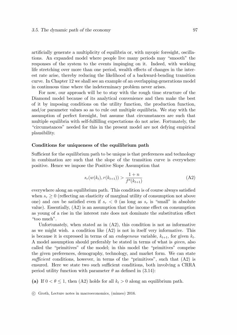
Suffi cient for the equilibrium path to be unique is that preferences and technologyin combination are such that the slope of the transition curve is everywherepositive. Hence we impose the Positive Slope Assumption that

sr(w(kt), r(kt+1)) >1 + n

f ′′(kt+1)(A2)

everywhere along an equilibrium path. This condition is of course always satisfiedwhen sr ≥ 0 (reflecting an elasticity of marginal utility of consumption not aboveone) and can be satisfied even if sr < 0 (as long as sr is “small” in absolutevalue). Essentially, (A2) is an assumption that the income effect on consumptionas young of a rise in the interest rate does not dominate the substitution effect“too much”.Unfortunately, when stated as in (A2), this condition is not as informative

as we might wish. a condition like (A2) is not in itself very informative. Thisis because it is expressed in terms of an endogenous variable, kt+1, for given kt.A model assumption should preferably be stated in terms of what is given, alsocalled the “primitives” of the model; in this model the “primitives” comprisethe given preferences, demography, technology, and market form. We can statesuffi cient conditions, however, in terms of the “primitives”, such that (A2) isensured. Here we state two such suffi cient conditions, both involving a CRRAperiod utility function with parameter θ as defined in (3.14):

(a) If 0 < θ ≤ 1, then (A2) holds for all kt > 0 along an equilibrium path.



(b) If the production function is of CES-type,18 i.e., f(k) = A(αkγ + 1− α)1/γ,A > 0, 0 < α < 1, −∞ < γ < 1, then (A2) holds along an equilibrium patheven for θ > 1, if the elasticity of substitution between capital and labor,1/(1− γ), is not too small, i.e., if

1

1− γ >1− 1/θ

1 + (1 + ρ)−1/θ(1 + f ′(k)− δ)(1−θ)/θ (3.36)

for all k > 0. In turn, suffi cient for this is that (1− γ)−1 > 1− θ−1.

That (a) is suffi cient for (A2) is immediately visible in (3.15). The suffi ciencyof (b) is proved in Appendix D. The elasticity of substitution between capitaland labor is a concept analogue to the elasticity of intertemporal substitutionin consumption. It is a measure of the sensitivity of the chosen k = K/L withrespect to the relative factor price. The next chapter goes more into detail withthe concept and shows, among other things, that the Cobb-Douglas productionfunction corresponds to γ = 0. So the Cobb-Douglas production function willsatisfy the inequality (1− γ)−1 > 1− θ−1 (since θ > 0), hence also the inequality(3.36).With these or other suffi cient conditions in the back of our mind we shall now

proceed imposing the Positive Slope Assumption (A2). To summarize:

PROPOSITION 3 (uniqueness of an equilibrium path) Suppose the No Fast andPositive Slope assumptions, (A1) and (A2), apply. Then:(i) if k0 > 0, there exists a unique equilibrium path;(ii) if k0 = 0, an equilibrium path exists if and only if f(0) > 0 (i.e., capital notessential).

When the conditions of Proposition 3 hold, the fundamental difference equa-tion, (3.32), of the model defines kt+1 as an implicit function of kt,

kt+1 = ϕ(kt),

for all kt > 0, where ϕ(kt) is called a transition function. The derivative of thisimplicit function is given by (3.34) with kt+1 on the right-hand side replaced byϕ(kt), i.e.,

ϕ′(kt) =sw (w (kt) , r (ϕ(kt)))w

′(kt)

1 + n− sr (w (kt) , r (ϕ(kt))) r′(ϕ(kt))> 0. (3.37)

The positivity for all kt > 0 is due to (A2). Example 2 above leads to a transitionfunction.18CES stands for Constant Elasticity of Substitution. The CES production function was

briefly considered in Section 2.1 and is considered in detail in Chapter 4.



Having determined the evolution of kt, we have in fact determined the evolu-tion of “everything”in the economy: the factor prices w(kt) and r(kt), the savingof the young st = s(w(kt), r(kt+1)), and the consumption by both the young andthe old. The mechanism behind the evolution of the economy is the Walrasian (orClassical) mechanism where prices, here wt and rt, always adjust so as to generatemarket clearing as if there were a Walrasian auctioneer and where expectationsalways adjust so as to be model consistent.

Existence and stability of a steady state?

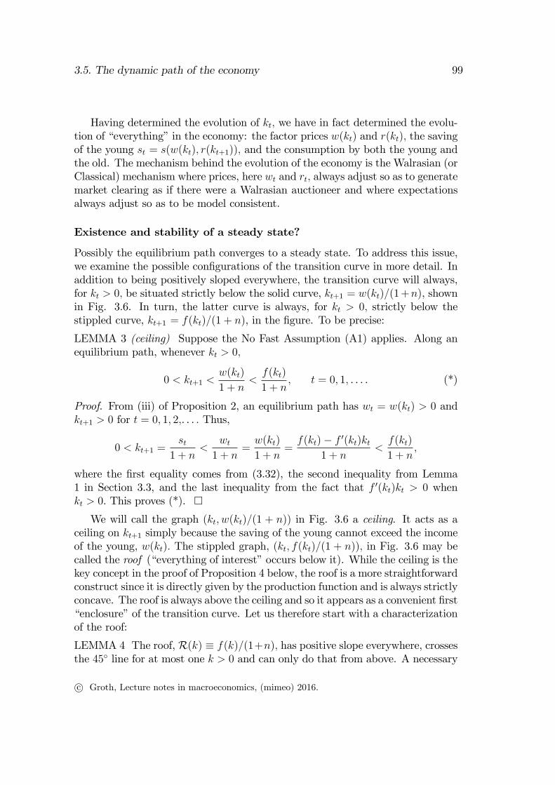
Possibly the equilibrium path converges to a steady state. To address this issue,we examine the possible configurations of the transition curve in more detail. Inaddition to being positively sloped everywhere, the transition curve will always,for kt > 0, be situated strictly below the solid curve, kt+1 = w(kt)/(1 +n), shownin Fig. 3.6. In turn, the latter curve is always, for kt > 0, strictly below thestippled curve, kt+1 = f(kt)/(1 + n), in the figure. To be precise:

LEMMA 3 (ceiling) Suppose the No Fast Assumption (A1) applies. Along anequilibrium path, whenever kt > 0,

0 < kt+1 <w(kt)

1 + n<f(kt)

1 + n, t = 0, 1, . . . . (*)

Proof. From (iii) of Proposition 2, an equilibrium path has wt = w(kt) > 0 andkt+1 > 0 for t = 0, 1, 2,. . . . Thus,

0 < kt+1 =st

1 + n<

wt1 + n

=w(kt)

1 + n=f(kt)− f ′(kt)kt

1 + n<f(kt)

1 + n,

where the first equality comes from (3.32), the second inequality from Lemma1 in Section 3.3, and the last inequality from the fact that f ′(kt)kt > 0 whenkt > 0. This proves (*). �We will call the graph (kt, w(kt)/(1 + n)) in Fig. 3.6 a ceiling. It acts as a

ceiling on kt+1 simply because the saving of the young cannot exceed the incomeof the young, w(kt). The stippled graph, (kt, f(kt)/(1 + n)), in Fig. 3.6 may becalled the roof (“everything of interest”occurs below it). While the ceiling is thekey concept in the proof of Proposition 4 below, the roof is a more straightforwardconstruct since it is directly given by the production function and is always strictlyconcave. The roof is always above the ceiling and so it appears as a convenient first“enclosure”of the transition curve. Let us therefore start with a characterizationof the roof:

LEMMA 4 The roof, R(k) ≡ f(k)/(1+n), has positive slope everywhere, crossesthe 45◦ line for at most one k > 0 and can only do that from above. A necessary



and suffi cient condition for the roof to be above the 45◦ line for small k is thateither limk→0 f

′(k) > 1 + n or f(0) > 0 (capital not essential).

Proof. Since f ′ > 0, the roof has positive slope. Since f ′′ < 0, it can only crossthe 45◦ line once and only from above. If and only if limk→0 f

′(k) > 1 + n, thenfor small kt, the roof is steeper than the 45◦ line. Obviously, if f(0) > 0, thenclose to the origin, the roof will be above the 45◦ line. �

Figure 3.6: A case where both the roof and the ceiling cross the 45◦ line, but thetransition curve does not (no steady state exists).

The ceiling is generally a more complex construct. It can have convex sectionsand for instance cross the 45◦ line at more than one point if at all. While theroof can be above the 45◦ line for all kt > 0, the ceiling cannot. Indeed, (ii) ofthe next lemma implies that if for small kt the ceiling is above the 45◦ line, theceiling will necessarily cross the 45◦ line at least once for larger kt.

LEMMA 5 Given w(k) = f(k) − f ′(k)k for all k ≥ 0, where f(k) satisfiesf(0) ≥ 0, f ′ > 0, f ′′ < 0, the following holds:(i) limk→∞w(k)/k = 0;(ii) the ceiling, C(k) ≡ w(k)/(1 + n), is positive and has positive slope for allk > 0; moreover, there exists k > 0 such that C(k) < k for all k > k.

Proof. (i) In view of f(0) ≥ 0 combined with f ′′ < 0, we have w(k) > 0 forall k > 0. Hence, limk→∞w(k)/k ≥ 0 if this limit exists. Consider an arbitrary



k1 > 0. We have f ′(k1) > 0. For all k > k1, it holds that 0 < f ′(k) < f ′(k1), inview of f ′ > 0 and f ′′ < 0, respectively. Hence, limk→∞ f

′(k) exists and

0 ≤ limk→∞

f ′(k) < f ′(k1). (3.38)

We have

limk→∞

w(k)

k= lim

k→∞

f(k)

k− lim

k→∞f ′(k). (3.39)

There are two cases to consider. Case 1: f(k) has an upper bound. Then,limk→∞ f(k)/k = 0 so that limk→∞w(k)/k = − limk→∞ f

′(k) = 0, by (3.39)and (3.38), as w(k)/k > 0 for all k > 0. Case 2: limk→∞ f(k) = ∞. Then,by L’Hôpital’s rule for “∞/∞”, limk→∞(f(k)/k) = limk→∞ f

′(k) so that (3.39)implies limk→∞w(k)/k = 0.(ii) As n > −1 and w(k) > 0 for all k > 0, C(k) > 0 for all k > 0. From

w′(k) = −kf ′′(k) > 0 follows C ′(k) = −kf ′′(k)/(1 + n) > 0 for all k > 0; that is,the ceiling has positive slope everywhere. For k > 0, the inequality C(k) < k isequivalent to w(k)/k < 1+n. By (i) follows that for all ε > 0, there exists kε > 0such that w(k)/k < ε for all k > kε. Now, letting ε = 1 + n and k = kε provesthat there exists k > 0 such that w(k)/k < 1 + n for all k > k. �A necessary condition for existence of a (non-trivial) steady state is that

the roof is above the 450 line for small kt. But this is not suffi cient for alsothe transition curve to be above the 450 line for small kt. Fig. 3.6 illustratesthis. Here the transition curve is in fact everywhere below the 450 line. Inthis case no steady state exists and the dynamics imply convergence towards the“catastrophic” point (0, 0). Given the rate of population growth, the saving ofthe young is not suffi cient to avoid famine in the long run. This outcome willoccur if the technology implies so low productivity that even when all incomeof the young were saved, we would have kt+1 < kt for all kt > 0, cf. Exercise3.2. The Malthusian mechanism will be at work and bring down n (outside themodel). This exemplifies that even a trivial steady state (the point (0,0)) maybe of interest in so far as it may be the point the economy is heading to (thoughnever reaching it).To help existence of a steady state we will impose the condition that either

capital is not essential or preferences and technology fit together in such a waythat the slope of the transition curve is larger than one for small kt. That is, weassume that either

(i) f(0) > 0 or (A3)

(ii) limk→0

ϕ′(k) > 1,

where ϕ′(k) is implicitly given in (3.37). Whether condition (i) of (A3) holds ina given situation can be directly checked from the production function. If it does



not, we should check condition (ii). But this condition is less amenable becausethe transition function ϕ is not one of the “primitives” of the model. Thereexist cases, though, where we can find an explicit transition function and try outwhether (ii) holds (like in Example 2 above). But generally we can not. Then wehave to resort to suffi cient conditions for (ii) of (A3), expressed in terms of the“primitives”. For example, if the period utility function belongs to the CRRAclass and the production function is Cobb-Douglas at least for small k, then (ii)of (A3) holds (see Appendix E). Anyway, as (i) and (ii) of (A3) can be interpretedas reflecting two different kinds of “early steepness”of the transition curve, weshall call (A3) the Early Steepness Assumption.19

Before stating the proposition aimed at, we need a definition of the conceptof asymptotic stability.

DEFINITION 5 Consider a first-order autonomous difference equation xt+1 =g(xt), t = 0, 1, 2, . . . . A steady state x∗ > 0 is (locally) asymptotically stable ifthere exists ε > 0 such that x0 ∈ (x∗− ε, x∗+ ε) implies that xt → x∗ for t→∞.A steady state x∗ > 0 is globally asymptotically stable if for all feasible x0 > 0, itholds that xt → x∗ for t→∞.

Applying this definition on our difference equation kt+1 = ϕ(kt), we have:

PROPOSITION 4 (existence and stability of a steady state) Assume that theNo Fast Assumption (A1) and the Positive Slope assumption (A2) apply as wellas the Early Steepness Assumption (A3). Then there exists at least one steadystate k∗1 > 0 that is locally asymptotically stable. If kt does not converge to k∗1,kt converges to another steady state. Oscillations do not occur.

Proof. By (A1), Lemma 3 applies. From Proposition 2 we know that if (i) of(A3) holds, then kt+1 = st/(1 + n) > 0 even for kt = 0. Alternatively, (ii) of (A3)is enough to ensure that the transition curve lies above the 45◦ line for small kt.According to (ii) of Lemma 5, for large kt the ceiling is below the 45◦ line. Beingbelow the ceiling, cf. Lemma 3, the transition curve must therefore cross the 45◦

line at least once. Let k∗1 denote the smallest kt at which it crosses. Then k∗1 > 0

is a steady state with the property 0 < ϕ′ (k∗1) < 1. By graphical inspection we seethat this steady state is asymptotically stable. If it is the only (non-trivial) steadystate, it is globally asymptotically stable. Otherwise, if kt does not converge tok∗1, kt converges to one of the other steady states. Indeed, divergence is ruled outsince, by Lemma 5, there exists k > 0 such that w(k)/(1 + n) < k for all k > k(Fig. 3.7 illustrates). For oscillations to come about there must exist a steadystate, k∗∗, with ϕ′ (k∗∗) < 0, but this is impossible in view of (A2). �

19In (i) of (A3), the “steepness” is rather a “hop”at k = 0 if we imagine k approaching nilfrom below.



Figure 3.7: A case of multiple steady states (and capital being not essential).

From Proposition 4 we conclude that, given k0, the assumptions (A1) - (A3)ensure existence and uniqueness of an equilibrium path; moreover, the equilibriumpath converges towards some steady state. Thus with these assumptions, for anyk0 > 0, sooner or later the system settles down at some steady state k∗ > 0. Forthe factor prices we therefore have

rt = f ′(kt)− δ → f ′(k∗)− δ ≡ r∗, and

wt = f(kt)− ktf ′(kt)→ f(k∗)− k∗f ′(k∗) ≡ w∗,

for t → ∞. But there may be more than one steady state and therefore onlylocal stability is guaranteed. This can be shown by examples, where the utilityfunction, the production function, and parameters are specified in accordancewith the assumptions (A1) - (A3) (see Exercise 3.5 and ...).Fig. 3.7 illustrates such a case (with f(0) > 0 so that capital is not essential).

Moving West-East in the figure, the first steady state, k∗1, is stable, the second,k∗2, unstable, and the third, k

∗3, stable. In which of the two stable steady states

the economy ends up depends on the initial capital-labor ratio, k0. The lowersteady state, k∗1, is known as a poverty trap. If 0 < k0 < k∗2, the economy iscaught in the trap and converges to the low steady state. But with high enoughk0 (k0 > k∗2), perhaps obtained by foreign aid, the economy avoids the trap andconverges to the high steady state. Looking back at Fig. 3.6, we can interpretthat figure’s scenario as exhibiting an inescapable poverty trap.



It turns out that CRRA utility combined with a Cobb-Douglas productionfunction ensures both that (A1) - (A3) hold and that a unique (non-trivial)steady state exists. So in this case global asymptotic stability of the steady stateis ensured.20 Example 2 and Fig. 3.4 above display a special case of this, thecase θ = 1.

This is of course a convenient case for the analyst. A Diamond model sat-isfying assumptions (A1) - (A3) and featuring a unique steady state is called awell-behaved Diamond model.

We end this section with the question: Is it possible that aggregate consump-tion, along an equilibrium path, for some periods exceeds aggregate income? Weshall see that this is indeed the case in this model if K0 (wealth of the old in theinitial period) is large enough. Indeed, from national accounting we have:

C10 + C20 = F (K0, L0)− I0 > F (K0, L0)⇔ I0 < 0

⇔ K1 < (1− δ)K0 ⇔ K0 −K1 > δK0.

So aggregate consumption in period 0 being greater than aggregate income isequivalent to a fall in the capital stock from period 0 to period 1 greater thanthe capital depreciation in period 0. Consider the log utility Cobb-Douglas casein Fig. 3.4 and suppose δ < 1 and Lt = L0 = 1, i.e., n = 0. Then kt = Kt for allt and by (3.35), Kt+1 = (1−α)A

2+ρKαt . Thus K1 < (1− δ)K0 for

K0 >

((1− α)A

(2 + ρ)(1− δ)

)1/(1−α)

.

As initial K is arbitrary, this situation is possible. When it occurs, it reflectsthat the financial wealth of the old is so large that their consumption (recallthey consume all their financial wealth as well as the interest on this wealth)exceeds what is left of current aggregate production after subtracting the amountconsumed by the young. So aggregate gross investment in the economy will benegative. Of course this is only feasible if capital goods can be “eaten”or at leastbe immediately (without further resources) converted into consumption goods.As it stands, the model has implicitly assumed this to be the case. And this is inline with the general setup since the output good is assumed homogeneous andcan either be consumed or piled up as capital.

We now turn to effi ciency problems.

20See last section of Appendix E.


3.6. The golden rule and dynamic ineffi ciency 105

3.6 The golden rule and dynamic ineffi ciency

An economy described by the Diamond model has the property that even thoughthere is perfect competition and no externalities, the outcome brought aboutby the market mechanism may not be Pareto optimal.21 Indeed, the economymay overaccumulate forever and thus suffer from a distinctive form of productionineffi ciency.A key element in understanding the concept of overaccumulation is the con-

cept of a golden-rule capital-labor ratio. Overaccumulation occurs when aggregatesaving maintains a capital-labor ratio above the golden-rule value forever. Let usconsider these concepts in detail.In the present section generally the period length is arbitrary except when

we relate to the Diamond model and the period length therefore is half of adultlifetime.

The golden-rule capital-labor ratio

The golden rule is a principle that relates to technically feasible paths. Theprinciple does not depend on the market form.Consider the economy-wide resource constraint Ct = Yt − St = F (Kt, Lt) −

(Kt+1−Kt+δKt), where we assume that F is neoclassical with CRS. Accordingly,aggregate consumption per unit of labor can be written

ct ≡CtLt

=F (Kt, Lt)− (Kt+1 −Kt + δKt)

Lt= f(kt) + (1− δ)kt − (1 + n)kt+1,

(3.40)where k is the capital-labor ratioK/L. Note that Ct will generally be greater thanthe workers’consumption. One should simply think of Ct as the flow of producedconsumption goods in the economy and ct as this flow divided by aggregate em-ployment, including the labor that in period t produces investment goods. Howthe consumption goods are distributed to different members of society is not ourconcern here.

DEFINITION 6 By the golden-rule capital-labor ratio, kGR, is meant that valueof the capital-labor ratio k, which results in the highest possible sustainable levelof consumption per unit of labor.

Sustainability requires replicability forever. We therefore consider a steady

21Recall that a Pareto optimal path is a technically feasible path with the property thatno other technically feasible path will make at least one individual better off without makingsomeone else worse off. A technically feasible path which is not Pareto optimal is called Paretoinferior.



state. In a steady state kt+1 = kt = k so that (3.40) simplifies to

c = f(k)− (δ + n)k ≡ c(k). (3.41)

Maximizing gives the first-order condition

c′(k) = f ′(k)− (δ + n) = 0. (3.42)

In view of c′′(k) = f ′′(k) < 0, the condition (3.42) is both necessary and suffi cientfor an interior maximum. Let us assume that δ + n > 0 and that f satisfies thecondition

limk→∞

f ′(k) < δ + n < limk→0

f ′(k).

Then (3.42) has a solution in k, and it is unique because c′′(k) < 0. The solutionis called kGR so that

f ′(kGR)− δ = n.

That is:

PROPOSITION 5 (the golden rule) The highest sustainable consumption levelper unit of labor in society is obtained when in steady state the net marginalproductivity of capital equals the growth rate of the economy.

Figure 3.8: A steady state with overaccumulation.

It follows that if a society aims at the highest sustainable level of consumptionand initially has k0 < kGR, society should increase its capital-labor ratio up to



the point where the extra output obtainable by a further small increase is exactlyoffset by the extra gross investment needed to maintain the capital-labor ratioat that level. The intuition is visible from (3.41). The golden-rule capital-laborratio, kGR, strikes the right balance in the trade-off between high output per unitof labor and a not too high investment requirement. Although a steady statewith k > kGR would imply higher output per unit of labor, it would also implythat a large part of that output is set aside for investment (namely the amount(δ + n)k per unit of labor) to counterbalance capital depreciation and growth inthe labor force; without this investment the high capital-labor ratio k∗ would notbe maintained. With k > kGR this feature would dominate the first effect so thatconsumption per unit of labor ends up low. Fig. 3.8 illustrates.The name golden rule hints at the golden rule from the Bible: “Do unto others

as you would have them to do unto you.”We imagine that God asks the newlyborn generation: “What capital-labor ratio would you prefer to be presentedwith, given that you must hand over the same capital-labor ratio to the nextgeneration?”The appropriate answer is: the golden-rule capital-labor ratio.

The possibility of overaccumulation in a competitive market economy

The equilibrium path in the Diamond model with perfect competition implies aninterest rate r∗ = f ′(k∗)− δ in a steady state. As an implication,

r∗ T n⇔ f ′(k∗)− δ T n⇔ k∗ S kGR, respectively,

in view of f ′′ < 0. Hence, a long-run interest rate below the growth rate of theeconomy indicates that k∗ > kGR. This amounts to a Pareto-inferior state ofaffairs. Indeed, everyone can be made better off if by a coordinated reduction ofsaving and investment, k is reduced. A formal demonstration of this is given inconnection with Proposition 6 in the next subsection. Here we give an accountin more intuitive terms.Consider Fig. 3.8. Let k be gradually reduced to the level kGR by refrain-

ing from investment in period t0 and forward until this level is reached. Whenthis happens, let k be maintained at the level kGR forever by providing for theneeded investment per young, (δ+ n)kGR. Then there would be higher aggregateconsumption in period t0 and every future period. Both the immediate reductionof saving and a resulting lower capital-labor ratio to be maintained contribute tothis result. There is thus scope for both young and old to consume more in everyfuture period.In the Diamond model a simple policy implementing such a Pareto improve-

ment in the case where k∗ > kGR (i.e., r∗ < n) is to incur a lump-sum tax onthe young, the revenue of which is immediately transferred lump sum to the old,



hence, fully consumed. Suppose this amounts to a transfer of one good from eachyoung to the old. Since there are 1 + n young people for each old person, everyold receives in this way 1 + n goods in the same period. Let this transfer berepeated every future period. By decreasing their saving by one unit, the youngcan maintain unchanged consumption in their youth, and when becoming old,they receive 1 + n goods from the next period’s young and so on. In effect, the“return”on the tax payment by the young is 1 + n next period. This is morethan the 1 + r∗ that could be obtained via the market through own saving.22

A proof that k∗ > kGR is indeed theoretically possible in the Diamond modelcan be based on the log utility-Cobb-Douglas case from Example 2 in Section3.5.3. As indicated by the formula for r∗ in that example, the outcome r∗ < n,which is equivalent to k∗ > kGR, can always be obtained by making the parameterα ∈ (0, 1) in the Cobb-Douglas function small enough. The intuition is that asmall α implies a high 1−α, that is, a high wage income wL = (1−α)KαL−α ·L= (1 − α)Y ; this leads to high saving by the young, since sw > 0. The result isa high kt+1 which generates a high real wage also next period and may in thismanner be sustained forever.An intuitive understanding of the fact that the perfectly competitive market

mechanism may thus lead to overaccumulation, can be based on the followingargument. Assume, first, that sr < 0. In this case, if the young in period texpects the rate of return on their saving to end up small (less than n), thedecided saving will be large in order to provide for consumption after retirement.But the aggregate result of this behavior is a high kt+1 and therefore a low f ′(kt+1).In this way the expectation of a low rt+1 is confirmed by the actual events. Theyoung persons each do the best they can as atomistic individuals, taking themarket conditions as given. Yet the aggregate outcome is an equilibrium withoveraccumulation, hence a Pareto-inferior outcome.Looking at the issue more closely, we see that sr < 0 is not crucial for this

outcome. Suppose sr = 0 (the log utility case) and that in the current period,kt is, for some historical reason, at least temporarily considerably above kGR.Thus, current wages are high, hence, st is relatively high (there is in this case nooffsetting effect on st from the relatively low expected rt+1). Again, the aggregateresult is a high kt+1 and thus the expectation is confirmed. Consequently, thesituation in the next period is the same and so on. By continuity, even if sr > 0,the argument goes through as long as sr is not too large.

22In this model with no utility of leisure, a tax on wage income, or a mandatory pay-as-you-gopension contribution (see Chapter 5), would act like a lump-sum tax on the young.The described tax-transfers policy will affect the equilibrium interest rate negatively. By

choosing an appropriate size of the tax this policy, combined with competitive markets, willunder certain conditions (see Chapter 5.1) bring the economy to the golden-rule steady statewhere overaccumulation has ceased and r∗ = n.



Dynamic ineffi ciency and the double infinity

Another name for the overaccumulation phenomenon is dynamic ineffi ciency.

DEFINITION 7 A technically feasible path {(ct, kt)}∞t=0 with the property thatthere does not exist another technically feasible path with higher ct in someperiods without smaller ct in other periods is called dynamically effi cient. Atechnically feasible path {(ct, kt)}∞t=0 which is not dynamically effi cient is calleddynamically ineffi cient.

PROPOSITION 6 A technically feasible path {(ct, kt)}∞t=0 with the property thatfor t→∞, kt → k∗ > kGR, is dynamically ineffi cient.

Proof. Let k∗ > kGR. Then there exists an ε > 0 such that k ∈ (k∗ − 2ε, k∗ + 2ε)implies f ′(k)− δ < n since f ′′ < 0. By concavity of f,

f(k)− f(k − ε) ≤ f ′(k − ε)ε. (3.43)

Consider a technically feasible path {(ct, kt)}∞t=0 with kt → k∗ for t → ∞ (thereference path). Then there exists a t0 such that for t ≥ t0, kt ∈ (k∗ − ε, k∗ + ε),f ′(kt) − δ < n and f ′(kt − ε) − δ < n. Consider an alternative feasible path{

(ct, kt)}∞t=0

, where a) for t = t0 consumption is increased relative to the reference

path such that kt0+1 = kt0 − ε; and b) for all t > t0, consumption is such thatkt+1 = kt− ε.We now show that after period t0, ct > ct. Indeed, for all t > t0, by(3.40),

ct = f(kt) + (1− δ)kt − (1 + n)kt+1

= f(kt − ε) + (1− δ)(kt − ε)− (1 + n)(kt+1 − ε)≥ f(kt)− f ′(kt − ε)ε+ (1− δ)(kt − ε)− (1 + n)(kt+1 − ε) (by (3.43))

> f(kt)− (δ + n)ε+ (1− δ)kt − (1 + n)kt+1 + (δ + n)ε

= f(kt) + (1− δ)kt − (1 + n)kt+1 = ct,

by (3.40). �Moreover, it can be shown23 that:

PROPOSITION 7 A technically feasible path {(ct, kt)}∞t=0 such that for t→∞,kt → k∗ ≤ kGR, is dynamically effi cient.

Accordingly, a steady state with k∗ < kGR is never dynamically ineffi cient.This is because increasing k from this level always has its price in terms of adecrease in current consumption; and at the same time decreasing k from this

23See Cass (1972).



level always has its price in terms of lost future consumption. But a steady statewith k∗ > kGR is always dynamically ineffi cient. Intuitively, staying forever withk = k∗ > kGR, implies that society never enjoys its great capacity for producingconsumption goods.The fact that k∗ > kGR − and therefore dynamic ineffi ciency− cannot be ruled

out might seem to contradict the First Welfare Theorem from the microeconomictheory of general equilibrium. This is the theorem saying that under certainconditions (essentially that increasing returns to scale are absent, markets arecompetitive, no goods are of public good character, and there are no externalities,then market equilibria are Pareto optimal. In fact, however, the First WelfareTheorem also presupposes a finite number of periods or, if the number of periodsis infinite, then a finite number of agents. In contrast, in the OLG model thereis a double infinity: an infinite number of periods and agents. Hence, the FirstWelfare Theorem breaks down. Indeed, the case r∗ < n, i.e., k∗ > kGR, can ariseunder laissez-faire. Then, as we have seen, everyone can be made better off by acoordinated intervention by some social arrangement (a government for instance)such that k is reduced.The essence of the matter is that the double infinity opens up for technically

feasible reallocations which are definitely beneficial when r∗ < n and which acentral authority can accomplish but the market can not. That nobody needloose by the described kind of redistribution is due to the double infinity: theeconomy goes on forever and there is no last generation. Nonetheless, some kindof centralized coordination is required to accomplish a solution.There is an analogy in “Gamow’s bed problem”: There are an infinite number

of inns along the road, each with one bed. On a certain rainy night all innkeepershave committed their beds. A late guest comes to the first inn and asks for abed. “Sorry, full up!”But the minister of welfare hears about it and suggeststhat from each inn one incumbent guest moves down the road one inn.24

Whether the theoretical possibility of overaccumulation should be a matter ofpractical concern is an empirical question about the relative size of rates of returnand economic growth. To answer the question meaningfully, we need an extensionof the criterion for overaccumulation so that the presence of technological progressand rising per capita consumption in the long run can be taken into account. Thisis one of the topics of the next chapter. At any rate, we can already here revealthat there exists no indication that overaccumulation has ever been an actualproblem in industrialized market economies.A final remark before concluding. Proposition 5 about the golden rule can be

generalized to the case where instead of one there are n different capital goods in

24George Gamow (1904-1968) was a Russian physicist. The problem is also known as Hilbert’shotel problem, after the German mathematician David Hilbert (1862-1943).


3.7. Concluding remarks 111

the economy. Essentially the generalization says that assuming CRS-neoclassicalproduction functions with n different capital goods as inputs, one consumptiongood, no technological change, and perfectly competitive markets, a steady statein which per-unit-of labor consumption is maximized has interest rate equal tothe growth rate of the labor force when technological progress is ignored (see,e.g., Mas-Colell, 1989).

3.7 Concluding remarks

(Unfinished)In several respects the conclusions we get from OLG models are different than

those from other neoclassical models, in particular representative agent models(to be studied later). In OLG models the aggregate quantities are the outcomeof the interplay of finite-lived agents at different stages in their life cycle. Theturnover in the population plays a crucial role. In this way the OLG approachlays bare the possibility of coordination failure on a grand scale. In contrast, in arepresentative agent model, aggregate quantities are just a multiple of the actionsof the representative household.Regarding analytical tractability, the complexity implied by having in every

period two different coexisting generations is in some respects more than compen-sated by the fact that the finite time horizon of the households make the dynamicsof the model one-dimensional : we end up with a first-order difference equationin the capital-labor ratio, kt, in the economy. In contrast, the dynamics of thebasic representative agent model (Chapter 8 and 10) is two-dimensional (owingto the assumed infinite horizon of the households considered as dynasties).Miscellaneous notes:OLG gives theoretical insights concerning macroeconomic implications of life

cycle behavior, allows heterogeneity, provides training in seeing the economy asconsisting of a heterogeneous population where the distribution of agent charac-teristics matters for the aggregate outcome.Farmer (1993), p. 125, notes that OLG models are diffi cult to apply and

for this reason much empirical work in applied general equilibrium theory hasregrettably instead taken the representative agent approach.Outlook: Rational speculative bubbles in general equilibrium, cf. Chapter ?.

3.8 Literature notes

1. The Nobel Laureate Paul A. Samuelson (1915-2009) is one of the pioneersof OLG models. Building on the French economist and Nobel laureate Maurice



Allais (1911-2010), a famous article by Samuelson, from 1958, is concerned witha missing market problem. Imagine a two-period OLG economy where, as in theDiamond model, only the young have an income (by Samuelson simplifying con-sidered an exogenous endowment of consumption goods from heaven). Contraryto the Diamond model, however, there is no capital. Also other potential stores ofvalue are absent. Then, in the laissez-faire market economy the old have to starvebecause they can no longer work and had no possibility of saving - transferringincome - as young.The allocation of resources in the economy is Pareto-inferior. Indeed, if each

member of the young generation hands over to the old generation one unit ofconsumption, and this is next period repeated by the new young generation andso on in the future, everyone will be better off. Since for every old there are 1 +nyoung, the implied rate of return would be n, the population growth rate. Suchtransfers do not arise under laissez-faire. A kind of social contract is required.As Samuelson pointed out, a government could in period 0 issue paper notes,“money”, and transfer these notes to the members of the old generation whowould then use them to buy goods from the young. Provided the young believedthe notes to be valuable in the next period, they would accept them in exchangefor some of their goods in order to use them in the next period for buying fromthe new young generation etc.We have here an example of how a social institution can solve a coordination

problem.25

2. Diamond (1965) extended Samuelson’s contribution by adding capital ac-cumulation. Because of its antecedents Diamonds OLGmodel is sometimes calledthe Samuelson-Diamond model or the Allais-Samuelson-Diamond model. In ourexposition we have drawn upon clarifications by Galor and Ryder (1989) andde la Croix and Michel (2002). The last mentioned contribution is an extensiveexploration of discrete-time OLG models and their applications. An advancedand thorough treatment from a microeconomic general equilibrium perspective iscontained in Bewley (2007).3. The life-cycle saving hypothesis was put forward by Franco Modigliani

(1918-2003) and associates in the 1950s. See for example Modigliani and Brum-berg (1954). Numerous extensions of the framework, relating to the motives (b)- (e) in the list of Section 3.1, see for instance de la Croix and Michel (2002).4. A review of the empirics of life-cycle behavior and attempts at refining

life-cycle models are given in Browning and Crossley (2001).5. Regarding the dynamic effi ciency issue, both the propositions 6 and 7 were

shown in a stronger form by the American economist David Cass (1937-2008).

25To just give a flavor of Samuelson’s contribution we have here ignored several aspects,including that Samuelson assumed three periods of life.


3.9. Appendix 113

Cass established the general necessary and suffi cient condition for a feasible path{(ct, kt)}∞t=0 to be dynamically effi cient (Cass 1972). Our propositions 6 and 7 aremore restrictive in that they are limited to paths that converge. Partly intuitiveexpositions of the deeper aspects of the theory are given by Shell (1971) andBurmeister (1980).6. Diamond has also contributed to other fields of economics, including search

theory for labor markets. In 2010 Diamond, together with Dale Mortensen andChristopher Pissarides, was awarded the Nobel price in economics.From here very incomplete:The two-period structure of Diamonds OLG model leaves little room for con-

sidering, e.g., education and dissaving in the early years of life. This kind of issuesis taken up in three-period extensions of the Diamond model, see de la Croix andMichell (2002).Multiple equilibria, self-fulfilling expectations, optimism and pessimism..Dynamic ineffi ciency, see also Burmeister (1980).Bewley 1977, 1980.Two-sector OLG: Galor (1992). Galor’s book on difference equations.On the golden rule in a general setup, see Mas-Colell (1989).

3.9 Appendix

A. On CRRA utility

Derivation of the CRRA function Consider a utility function u(c), definedfor all c > 0 and satisfying u′(c) > 0, u′′(c) < 0. Let the absolute value ofthe elasticity of marginal utility be denoted θ(c), that is, θ(c) ≡ −cu′′(c)/u′(c)> 0. We claim that if θ(c) is a positive constant, θ, then, up to a positive lineartransformation, u(c) must be of the form

u(c) =

{c1−θ

1−θ , when θ 6= 1,

ln c, when θ = 1,(*)

i.e., of CRRA form.

Proof. Suppose θ(c) = θ > 0. Then, u′′(c)/u′(c) = −θ/c. By integration, lnu′(c)= −θ ln c+A, where A is an arbitrary constant. Take the antilogarithm functionon both sides to get u′(c) = eAe−θ ln c = eAc−θ. By integration we get

u(c) =

{eA c

1−θ

1−θ +B, when θ 6= 1,

eA ln c+B, when θ = 1,

where B is an arbitrary constant. This proves the claim. Letting A = B = 0, weget (*). �



When we want to make the kinship between the members of the “CRRAfamily”transparent, we maintain A = 0 and for θ = 1 also B = 0, whereas forθ 6= 1 we set B = −1/(1 − θ). In this way we achieve that all members of theCRRA family will be represented by curves going through the same point as thelog function, namely the point (1, 0), cf. Fig. 3.2. For a particular θ > 0, θ 6= 1,we have u(c) = (c1−θ − 1)/(1 − θ), which makes up the CRRA utility functionin normalized form. Given θ, the transformation to normalized form is of noconsequence for the economic behavior since adding or subtracting a constantdoes not affect marginal rates of substitution.

The domain of the CRRA function We want to extend the domain toinclude c = 0. If θ ≥ 1, the CRRA function, whether in the form u(c) = (c1−θ −1)/(1 − θ) or in the form (*), is defined only for c > 0, not for c = 0. This isbecause for c→ 0 we get u(c)→ −∞. In this case we simply define u(0) = −∞.This will create no problems since the CRRA function anyway has the propertythat u′(c) → ∞, when c → 0 (whether θ is larger or smaller than one). Themarginal utility thus becomes very large as c becomes very small, that is, theNo Fast Assumption is satisfied. This will ensure that the chosen c is strictlypositive whenever there is a positive budget. So throughout this book we definethe domain of the CRRA function to be [0,∞) .

The range of the CRRA function Considering the CRRA function u(c) ≡(c1−θ − 1

)(1− θ)−1 for c ∈ [0,∞) , we have:

for 0 < θ < 1, the range of u(c) is[−(1− θ)−1,∞

),

for θ = 1, the range of u(c) is [−∞,∞) ,

for θ > 1, the range of u(c) is [−∞,−(1− θ)−1).

Thus, in the latter case u(c) is bounded from above and so allows asymptotic“saturation”to occur.

B. Deriving the elasticity of intertemporal substitution in consumption

Referring to Section 3.3, we here show that the definition of σ(c1, c2) in (3.17)gives the result (3.18). Let x ≡ c2/c1 and β ≡ (1 + ρ)−1. Then the first-ordercondition (3.16) and the equation describing the considered indifference curveconstitute a system of two equations

u′(c1) = βu′(xc1)R,

u(c1) + βu(xc1) = U .


3.9. Appendix 115

For a fixed utility level U = U these equations define c1 and x as implicit functionsof R, c1 = c(R) and x = x(R). We calculate the total derivative with respect toR in both equations and get, after ordering,

[u′′(c1)− βRu′′(xc1)x] c′(R)− βRu′′(xc1)c1x′(R)

= βu′(xc1), (3.44)

[u′(c1) + βu′(xc1)x] c′(R) = −βu′(xc1)c1x′(R). (3.45)

Substituting c′(R) from (3.45) into (3.44) and ordering now yields

−[xc1u′′(c1)

u′(c1)+R

xc1u′′(xc1)

u′(xc1)

]R

xx′(R) = x+R.

Since −cu′′(c)/u′(c) ≡ θ(c), this can be written

R

xx′(R) =

x+R

xθ(c1) +Rθ(xc1).

Finally, in view of xc1 = c2 and the definition of σ(c1, c2), this gives (3.18).

C. Walras’law

In the proof of Proposition 1 we referred to Walras’law. Here is how Walras’lawworks in each period in a model like this. We consider period t, but for simplicitywe skip the time index t on the variables. There are three markets, a marketfor capital services, a market for labor services, and a market for output goods.Suppose a “Walrasian auctioneer”calls out the price vector (r, w, 1), where r > 0and w > 0, and asks all agents, i.e., the young, the old, and the representativefirm, to declare their supplies and demands.The supplies of capital and labor are by assumption inelastic and equal to K

units of capital services and L units of labor services. But the demand for capitaland labor services depends on the announced r and w. Let the potential pureprofit of the representative firm be denoted Π. If r and w are so that Π < 0, thefirm declares Kd = 0 and Ld = 0. If on the other hand at the announced r andw, Π = 0 (as when r = r(k) + δ and w = w(k)), the desired capital-labor ratio isgiven as kd = f ′−1(r) from (3.20), but the firm is indifferent with respect to theabsolute level of the factor inputs. In this situation the auctioneer tells the firmto declare Ld = L (recall L is the given labor supply) and Kd = kdLd which iscertainly acceptable for the firm. Finally, if Π > 0, the firm is tempted to declareinfinite factor demands, but to avoid that, the auctioneer imposes the rule thatthe maximum allowed demands for capital and labor are 2K and 2L, respectively.



Within these constraints the factor demands will be uniquely determined by rand w and we have

Π = Π(r, w, 1) = F (Kd, Ld)− rKd − wLd. (3.46)

The owners of both the capital stock K and the representative firm must bethose who saved in the previous period, namely the currently old. These elderlywill together declare the consumption c2L−1 = (1 + r − δ)K + Π and the netinvestment −K (which amounts to disinvestment). The young will declare theconsumption c1L = wL− s(w, re+1)L and the net investment sL = s(w, re+1)L. Soaggregate declared consumption will be C = (1 + r− δ)K + Π +wL− s(w, re+1)Land aggregate net investment I − δK = s(w, re+1)L − K. It follows that C + I= wL + rK + Π. The aggregate declared supply of output is Y s = F (Kd, Ld).The values of excess demands in the three markets now add to

Z(r, w, 1) ≡ w(Ld − L) + r(Kd −K) + C + I − Y s

= wLd − wL+ rKd − rK + wL+ rK + Π− F (Kd, Ld)

= wLd + rKd + Π− F (Kd, Ld) = 0,

by (3.46).This is a manifestation of Walras’law for each period: whatever the announced

price vector for the period is, the aggregate value of excess demands in the periodis zero. The reason is the following. When each household satisfies its budgetconstraint and each firm pays out its ex ante profit,26 then the economy as awhole has to satisfy an aggregate budget constraint for the period considered.The budget constraints, demands, and supplies operating in this thought ex-

periment (and in Walras’law in general) are the Walrasian budget constraints,demands, and supplies. Outside equilibrium these are somewhat artificial con-structs. A Walrasian budget constraint is based on the assumption that thedesired actions can be realized. This assumption will be wrong unless r and ware already at their equilibrium levels. But the assumption that desired actionscan be realized is never falsified because the thought experiment does not allowtrades to take place outside Walrasian equilibrium. Similarly, the Walrasian con-sumption demand by the worker is rather hypothetical outside equilibrium. Thisdemand is based on the income the worker would get if fully employed at theannounced real wage, not on the actual employment (or unemployment) at thatreal wage.These ambiguities notwithstanding, the important message of Walras’ law

goes through, namely that when two of the three markets clear (in the sense ofthe Walrasian excess demands being nil), so does the third.

26By ex ante profit is meant the hypothetical profit calculated on the basis of firms’desiredsupply evaluated at the announced price vector, (r, w, 1).


3.9. Appendix 117

D. Proof of (i) and (ii) of Proposition 2

For convenience we repeat the fundamental difference equation characterizing anequilibrium path:

kt+1 =s (w (kt) , r (kt+1))

1 + n,

where w(k) ≡ f(k)− f ′(k)k > 0 for all k > 0 and r(k) ≡ f ′(k)− δ > −1 for allk ≥ 0. The key to the proof of Proposition 2 about existence of an equilibriumpath is the following lemma.

LEMMA D1 Suppose the No Fast Assumption (A1) applies and let w > 0 andn > −1 be given. Then the equation

s (w, r (k))

k= 1 + n. (3.47)

has at least one solution k > 0.

Proof. Note that 1 + n > 0. From Lemma 1 in Section 3.3 follows that for allpossible values of r(k), 0 < s(w, r(k)) < w. Hence, for any k > 0,

0 <s (w, r (k))

k<w

k.

Letting k → ∞ we then have s (w, r (k)) /k → 0 since s (w, r (k)) /k is squeezedbetween 0 and 0 (as indicated in the two graphs in Fig. 3.9).

Figure 3.9: Existence of a solution to equation (3.47).

Next we consider k → 0. There are two cases.Case 1: limk→0 s (w, r (k)) > 0.27 Then obviously limk→0 s (w, r (k)) /k =∞.

27If the limit does not exist, the proof applies to the limit inferior of s (w, r (k)) for k → 0.The limit inferior for i→∞ of a sequence {xi}∞i=0 is defined as limi→∞ inf {xj | j = i, i+1, . . . } ,where inf of a set Si = {xj | j = i, i+ 1, . . . } is defined as the greatest lower bound for Si.



Case 2: limk→0 s (w, r (k)) = 0.28 In this case we have

limk→0

r (k) =∞. (3.48)

Indeed, since f ′(k) rises monotonically as k → 0, the only alternative would bethat limk→0 r (k) exists and is <∞; then, by Lemma 1 in Section 3.3, we wouldbe in case 1 rather than case 2. By the second-period budget constraint, withr = r(k), consumption as old is c2 = s (w, r (k)) (1 + r(k)) ≡ c(w, k) > 0 so that

s (w, r (k))

k=

c(w, k)

[1 + r(k)] k.

The right-hand side of this equation goes to∞ for k → 0 since limk→0 [1 + r(k)] k =0 by Technical Remark in Section 3.4 and limk→0 c(w, k) = ∞; this latter factfollows from the first-order condition (3.8), which can be written

0 ≤ u′(c(w, k)) = (1 + ρ)u′(w − s(w, r(k))

1 + r(k)≤ (1 + ρ)

u′(w)

1 + r(k).

Taking limits on both sides gives

limk→0

u′(c(w, k)) = (1 + ρ) limk→0

u′(w − s (w, r (k)))

1 + r(k)= (1 + ρ) lim

k→0

u′(w)

1 + r(k)= 0,

where the second equality comes from the fact that we are in case 2 and thethird comes from (3.48). But since u′(c) > 0 and u′′(c) < 0 for all c > 0,limk→0 u

′(c(w, k)) = 0 requires limk→0 c(w, k) =∞, as was to be shown.In both Case 1 and Case 2 we thus have that k → 0 implies s (w, r (k)) /k →

∞. Since s (w, r (k)) /k is a continuous function of k, there must be at least onek > 0 such that (3.47) holds (as illustrated by the two graphs in Fig. 3.14). �Now, to prove (i) of Proposition 2, consider an arbitrary kt > 0. We have

w(kt) > 0. In (3.47), let w = w(kt). By Lemma C1, (3.47) has a solution k > 0.Set kt+1 = k. Starting with t = 0, from a given k0 > 0 we thus find a k1 > 0 andletting t = 1, from the now given k1 we find a k2 and so on. The resulting infinitesequence {kt}∞t=0 is an equilibrium path. In this way we have proved existence ofan equilibrium path if k0 > 0. Thereby (i) of Proposition 2 is proved.But what if k0 = 0? Then, if f(0) = 0, no temporary equilibrium is possible in

period 0, in view of (ii) of Proposition 1; hence there can be no equilibrium path.Suppose f(0) > 0. Then w(k0) = w(0) = f(0) > 0, as explained in TechnicalRemark in Section 3.4. Let w in equation (3.47) be equal to f(0). By LemmaC1 this equation has a solution k > 0. Set k1 = k. Letting period 1 be the newinitial period, we are back in the case with initial capital positive. This proves(ii) of Proposition 2.

28If the limit does not exist, the proof applies to the limit inferior of s (w, r (k)) for k → 0.


3.9. Appendix 119

E. Suffi cient conditions for certain properties of the transition curve

Positive slope everywhere For convenience we repeat here the condition(3.36):

1

1− γ >1− σ

1 + (1 + ρ)−σ(1 + f ′(k)− δ)σ−1, (*)

where we have substituted σ ≡ 1/θ. In Section 3.5.3 we claimed that in theCRRA-CES case this condition is suffi cient for the transition curve to be posi-tively sloped everywhere. We here prove the claim.Consider an arbitrary kt > 0 and let w ≡ w(kt) > 0. Knowing that w′(kt) > 0

for all kt > 0, we can regard kt+1 as directly linked to w. With k representingkt+1, k must satisfy the equation k = s(w, r(k))/(1 + n). A suffi cient conditionfor this equation to implicitly define k as an increasing function of w is also asuffi cient condition for the transition curve to be positively sloped for all kt > 0.When u(c) belongs to the CRRA class, by (3.15) with σ ≡ 1/θ, we have

s(w, r(k)) = [1 + (1 + ρ)σ(1 + r(k))1−σ]−1w. The equation k = s(w, r(k))/(1+n)

then impliesw

1 + n= k

[1 + (1 + ρ)σR(k)1−σ] ≡ h(k), (3.49)

where R(k) ≡ 1 + r(k) ≡ 1 + f ′(k)− δ > 0 for all k > 0. It remains to provide asuffi cient condition for obtaining h′(k) > 0 for all k > 0. We have

h′(k) = 1 + (1 + ρ)σR(k)1−σ [1− (1− σ)η(k)] , (3.50)

since η(k) ≡ −kR′(k)/R(k) > 0, the sign being due to R′(k) = f ′′(k) < 0. Soh′(k) > 0 if and only if 1−(1−σ)η(k) > −(1+ρ)−σR(k)σ−1, a condition equivalentto

1

η(k)>

1− σ1 + (1 + ρ)−σR(k)σ−1

. (3.51)

To make this condition more concrete, consider the CES production function

f(k) = A(αkγ + 1− α), A > 0, 0 < α < 1, γ < 1. (3.52)

Then f ′(k) = αAγ(f(k)/k)1−γ and defining π(k) ≡ f ′(k)k/f(k) we find

η(k) = (1− γ)(1− π(k))f ′(k)

1− δ + f ′(k)≤ (1− γ)(1− π(k)) < 1− γ, (3.53)

where the first inequality is due to 0 ≤ δ ≤ 1 and the second to 0 < π(k) < 1,which is an implication of strict concavity of f combined with f(0) ≥ 0. Thus,η(k)−1 > (1 − γ)−1 so that if (*) holds for all k > 0, then so does (3.51), i.e.,h′(k) > 0 for all k > 0. We have hereby shown that (*) is suffi cient for thetransition curve to be positively sloped everywhere.



Transition curve steep for k small Here we specialize further and considerthe CRRA-Cobb-Douglas case: u(c) = (c1−θ−1)/(1−θ), θ > 0, and f(k) = Akα,A > 0, 0 < α < 1. In the prelude to Proposition 4 in Section 3.5 it was claimedthat if this combined utility and technology condition holds at least for small k,then (ii) of (A3) is satisfied. We now show this.Letting γ → 0 in (3.52) gives the Cobb-Douglas function f(k) = Akα (this

is proved in the appendix to Chapter 4). With γ = 0, clearly (1 − γ)−1 = 1> 1 − σ, where σ ≡ θ−1 > 0. This inequality implies that (*) above holds andso the transition curve is positively sloped everywhere. As an implication thereis a transition function, ϕ, such that kt+1 = ϕ(kt), ϕ

′(kt) > 0. Moreover, sincef(0) = 0, we have, by Lemma 5, limkt→0 ϕ(kt) = 0.Given the imposed CRRA utility, the fundamental difference equation of the

model is

kt+1 =w(kt)

(1 + n) [1 + (1 + ρ)σR(kt+1)1−σ](3.54)

or, equivalently,

h(kt+1) =w(kt)

1 + n,

where h(kt+t) is defined as in (3.49). By implicit differentiation we find h′(kt+1)ϕ′(kt)= w′(kt)/(1 + n), i.e.,

ϕ′(kt) =w′(kt)

(1 + n)h′(kt+1)> 0.

If k∗ > 0 is a steady-state value of kt, (3.54) implies

1 + (1 + ρ)σR(k∗)1−σ =w(k∗)

(1 + n)k∗, (3.55)

and the slope of the transition curve at the steady state will be

ϕ′(k∗) =w′(k∗)

(1 + n)h′(k∗)> 0. (3.56)

If we can show that such a k∗ > 0 exists, is unique, and implies ϕ′(k∗) < 1, thenthe transition curve crosses the 45◦ line from above, and so (ii) of (A3) follows inview of limkt→0 = 0.Defining x(k) ≡ f(k)/k = Akα−1, where x′(k) = (α− 1)Akα−2 < 0, and using

that f(k) = Akα, we have R(k) = 1 + αx(k) − δ and w(k)/k = (1 − α)x(k).Hence, (3.55) can be written

1 + (1 + ρ)σ(1 + αx∗ − δ)1−σ =1− α1 + n

x∗, (3.57)


3.10. Exercises 121

where x∗ = x(k∗). It is easy to show graphically that this equation has a uniquesolution x∗ > 0 whether σ < 1, σ = 1, or σ > 1. Then k∗ = (x∗/A)1/(α−1) > 0 isalso unique.By (3.50) and (3.57),

h′(k∗) = 1 + (1− α1 + n

x∗ − 1) [1− (1− σ)η(k∗)] > 1 + (1− α1 + n

x∗ − 1)(1− η(k∗))

≥ 1 + (1− α1 + n

x∗ − 1)α,

where the first inequality is due to σ > 0 and the second to the fact that η(k) ≤1− α in view of (3.53) with γ = 0 and π(k) = α. Substituting this together withw′(k∗) = (1− α)αx∗ into (3.56) gives

0 < ϕ′(k∗) <αx∗

1 + n+ αx∗< 1, (3.58)

as was to be shown.

The CRRA-Cobb-Douglas case is well-behaved For the case of CRRAutility and Cobb-Douglas technology with CRS, existence and uniqueness of asteady state has just been proved. Asymptotic stability follows from (3.58). Sothe CRRA-Cobb-Douglas case is well-behaved.

3.10 Exercises

3.1 The dynamic accounting relation for a closed economy is

Kt+1 = Kt + SN (*)

where Kt is the aggregate capital stock and SNt is aggregate net saving. In theDiamond model, let S1t be aggregate net saving of the young in period t andS2t aggregate net saving of the old in the same period. On the basis of (*)give a direct proof that the link between two successive periods takes the formkt+1 = st/(1+n), where st is the saving of each young, n is the population growthrate, and kt+1 is the capital/labor ratio at the beginning of period t + 1. Hint:by definition, the increase in financial wealth is the same as net saving (ignoringgifts).

3.2 Suppose the production function in Diamond’s OLG model is Y = A(αKγ +(1−α)Lγ)1/γ, A > 0, 0 < α < 1, γ < 0, and Aα1/γ < 1+n. a) Given k ≡ K/L, findthe equilibrium real wage, w(k). b) Show that w(k) < (1+n)k for all k > 0. Hint:



consider the roof. c) Comment on the implication for the long-run evolution ofthe economy. Hint: consider the ceiling.

3.3 (multiple temporary equilibria with self-fulfilling expectations) Fig. 3.10shows the transition curve for a Diamond OLG model with u(c) = c1−θ/(1− θ),θ = 8, ρ = 0.4, n = 0.2, δ = 0.6, f(k) = A(bkp + 1 − b)1/p, A = 7, b = 0.33,p = −0.4.

a) Let t = 0. For a given k0 slightly below 1, how many temporary equilibriawith self-fulfilling expectations are there?

b) Suppose the young in period 0 expect the real interest rate on their savingto be relatively low. Describe by words the resulting equilibrium path inthis case. Comment (what is the economic intuition behind the path?).

c) In the first sentence under b), replace “low”by “high”. How is the answerto b) affected? What kind of diffi culty arises?

Figure 3.10: Transition curve for Diamond’s OLG model in the case described in Ex-ercise 3.3.

3.4 (plotting the transition curve by MATLAB) This exercise requires compu-tation on a computer. You may use MATLAB OLG program.29

29Made by Marc P. B. Klemp and available at the address:


3.10. Exercises 123

a) Enter the model specification from Exercise 3.3 and plot the transitioncurve.

b) Plot examples for two other values of the substitution parameter: p = −1.0and p = 0.5. Comment.

c) Find the approximate largest lower bound for p such that higher values ofp eliminates multiple equilibria.

d) In continuation of c), what is the corresponding elasticity of factor substi-tution, ψ? Hint: as shown in §4.4, the formula is ψ = 1/(1− p).

e) The empirical evidence for industrialized countries suggests that 0.4 < ψ <1.0. Is your ψ from d) empirically realistic? Comment.

3.5 (one stable and one unstable steady state) Consider the following Diamondmodel: u(c) = ln c, ρ = 2.3, n = 2.097, δ = 1.0, f(k) = A(bkp + 1− b)1/p, A = 20,b = 0.5, p = −1.0.

a) Plot the transition curve of the model. Hint: you may use either a programlike MATLAB OLG Program (available on the course website) or first alittle algebra and then Excel (or similar simple software).

b) Comment on the result you get. Will there exist a poverty trap? Why orwhy not?

c) At the stable steady state calculate numerically the output-capital ratio,the aggregate saving-income ratio, the real interest rate, and the capitalincome share of gross national income.

d) Briefly discuss how your results in c) comply with your knowledge of cor-responding empirical magnitudes in industrialized Western countries?

e) There is one feature which this model, as a long-run model, ought to incor-porate, but does not. Extend the model, taking this feature into account,and write down the fundamental difference equation for the extended modelin algebraic form.

f) Plot the new transition curve. Hint: given the model specification, thisshould be straightforward if you use Excel (or similar); and if you use MAT-LAB OLG Program, note that by a simple “trick”you can transform yournew model into the “old”form.

http://www.econ.ku.dk/okocg/Computation/.



g) The current version of the MATLAB OLG Program is not adapted to thisquestion. So at least here you need another approach, for instance based ona little algebra and then Excel (or similar simple software). Given k0 = 10,calculate numerically the time path of kt and plot the time profile of kt, i.e.,the graph (t, kt) in the tk-plane. Next, do the same for k0 = 1. Comment.

3.6 (dynamics under myopic foresight)(incomplete) Show the possibility of a chaotic trajectory.

3.7 Given the period utility function is CRRA, derive the saving function of theyoung in Diamond’s OLG model. Hint: substitute the period budget constraintsinto the Euler equation.

3.8 Short questions a) A steady-state capital-labor ratio can be in the “dy-namically effi cient” region or in the “dynamically ineffi cient” region. How arethe two mentioned regions defined? b) Give a simple characterization of the tworegions. c) The First Welfare Theorem states that, given certain conditions, anycompetitive equilibrium (≡Walrasian equilibrium) is Pareto optimal. Give a listof circumstances that each tend to obstruct Pareto optimality of a competitiveequilibrium.

3.9 Consider a Diamond OLG model for a closed economy. Let the utilitydiscount rate be denoted ρ and let the period utility function be specified asu (c) = ln c.

a) Derive the saving function of the young. Comment.

b) Let the aggregate production function be a neoclassical production functionwith CRS and ignore technological progress. Let Lt denote the number ofyoung in period t. Derive the fundamental difference equation of the model.

From now, assume that the production function is Y = αL+ βKL/(K + L),where α > 0 and β > 0 (as in Problem 2.4).

c) Draw a transition diagram illustrating the dynamics of the economy. Makesure that you draw the diagram so as to exhibit consistency with the pro-duction function.

d) Given the above information, can we be sure that there exists a unique andglobally asymptotically stable steady state? Why or why not?

e) Suppose the economy is in a steady state up to and including period t0 > 0.Then, at the shift from period t0 to period t0 + 1, a negative technologyshock occurs such that the technology level in period t0 + 1 is below that ofperiod t0. Illustrate by a transition diagram the evolution of the economyfrom period t0 onward. Comment.


3.10. Exercises 125

f) Let k ≡ K/L. In the (t, ln k) plane, draw a graph of ln kt such that thequalitative features of the time path of ln k before and after the shock,including the long run, are exhibited.

g) How, if at all, is the real interest rate in the long run affected by the shock?

h) How, if at all, is the real wage in the long run affected by the shock?

i) How, if at all, is the labor income share of national income in the long runaffected by the shock?

j) Explain by words the economic intuition behind your results in h) and i).

3.10




Documents

Chapter 3 The basic OLG model: Diamondweb.econ.ku.dk/okocg/MAT-OEK/MakØk2/MakØk2-2016...68 CHAPTER 3. THE BASIC OLG MODEL: DIAMOND The model takes elementary forms of heterogeneity