CHAPTER 3CHAPTER 3

ROOTS OF EQUATION

Presenter: Dr. Zalilah Sharer

© 2018 School of Chemical and Energy Engineering

Universiti Teknologi Malaysia

23 September 2018

Roots of equationGiven:

To solve: use the quadratic formula eq:

2( ) 0f x ax bx c= + + =

2 4b b ac− ± −=

Eqn. 3.1

Eqn. 3.2

• The values calculated by equation 3.2 are called the “roots” of

equation 3.1. They represent the values of x that make

equation 3.1 equal to zero.

• Roots of equations can be defined as “ the value of x that

makes f(x) = 0” or can be called as the zeros of the equation.

4

2

b b acx

a

− ± −= Eqn. 3.2

Solve f(x) = 0 for x

f(x)

x

Illustrations of places of roots

f(x)

x

f(x)

x

No rootsOne root

f(x)

x

x

f(x)

x

x

xl xu

Odd # of root

Even # of roots

• Example: The Newton’s 2nd Law for the parachutist’s

velocity.

• If the parameters are known, equation 3.3 can be used to

predict the parachutist’s velocity as a function of time.

v =gm

c1 − e

c

mt

Eqn. 3.3

predict the parachutist’s velocity as a function of time.

• Although the equation provides a mathematical

representation of the interrelationship among the model

variables & parameters, it cannot be solved for the drag

coefficient, c.

• The solution to the dilemma is provided by NM for roots of

equations.

vec

gmcf

tm

c

−

−=

−

1)( Eqn. 3.4

2 Types of Method to determine Root

of Equation

1. Bracketing methods (two initial guesses for the root are

required and these guesses must be “bracket”.)

a) Graphical method

b) Bisection Methodb) Bisection Method

c) False-Position Method

2. Open methods

a) Simple fixed-point iteration method

b) Newton- Raphson method

c) Secant Method

CHAPTER 3aCHAPTER 3a

BRACKETING METHOD

Bracketing method – a) Graphical

• Two initial guesses for the root are required

• Guesses must be “bracket”, or be on either side of

the root

“Obtaining an estimate of the root of an equation

f(x) = 0 by making a plot of the function. The point

at which it crosses the axis, represents the x value

for which f(x) = 0, provides a rough approximation

of the root”.

Example 1

Use the graphical approach to determine the drag

coefficient c needed for a parachutist of mass m =

68.1kg to have a velocity of 40 m/s after free falling68.1kg to have a velocity of 40 m/s after free falling

for time t = 10s. Step size is 4.

Note: the acceleration due to gravity is 9.8 m/s2

Solution• Given formula:

• Then, subtracting the dependent variable, v from

both side of the equation to give:

v =gm

c1 − e

c

mt

gmc

• Substitute all given values;

( / 68.1)10

0.146843

9.8(68.1)( ) (1 ) 40

or

667.38( ) (1 ) 40

c

c

f c ec

f c ec

−

−

= − −

= − −

vec

gmcf

tm

c

−

−=

−

1)(

Eqn. 5.1.1

Substitute various c values into the Eq E5.1.1:

C f(c)

4

8

12

34.115

17.653

6.067 The sign changes

Plot a graph : resulting curve crosses the c axis between 12

and 16. Rough estimate of the root ≅14.75

12

16

20

6.067

-2.269

-8.401

The graphical approach for determining the roots of an

equation.

Validity of the graphical estimate check by substitute c=

14.75 into equation.

0.146843 (14.75667.38( ) (1 ) 40

14.75

0.059 0

f c e−= − −

= ≅

• It can also be checked by substituting c =

14.75 into equation 3.3 to give:

v = 9.8 (68.1)/14.75 (1 – e –(14.75/68.1)10 )

v = 40.059 m/s

which is very close to desire fall velocity of

40 m/s.

b) Bisection method

• When applying graphical method, f(x) has changed sign

from +ve to –ve, where;

f(xl).f(xu) < 0

• Then there is at least one real root between x and x .• Then there is at least one real root between xl and xu.

• In this method, we dividing halve the interval (xl and xu )

into a number of sub-intervals. Each sub-interval is to locate

the sign changes. Alternatively, called binary chopping

(interval halving)

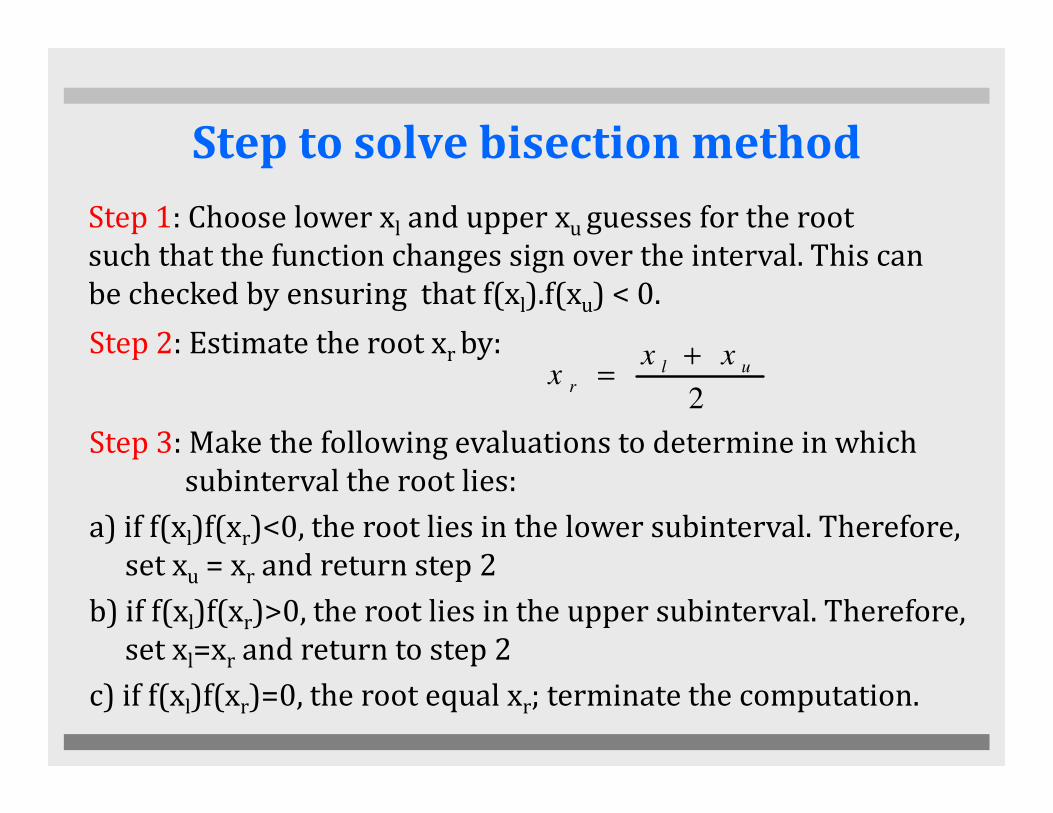
Step to solve bisection method

Step 1: Choose lower xl and upper xu guesses for the root

such that the function changes sign over the interval. This can

be checked by ensuring that f(xl).f(xu) < 0.

Step 2: Estimate the root xr by:

2

l ur

x xx

+=

Step 3: Make the following evaluations to determine in which

subinterval the root lies:

a) if f(xl)f(xr)<0, the root lies in the lower subinterval. Therefore,

set xu = xr and return step 2

b) if f(xl)f(xr)>0, the root lies in the upper subinterval. Therefore,

set xl=xr and return to step 2

c) if f(xl)f(xr)=0, the root equal xr; terminate the computation.

2

Example 2

Using bisection method to solve the same problem

approach as in graphical method. True value

given=14.7802

Solution• The first step in bisection method is to guess two values

of the unknown (xl and xu) where the function changes.

• As from the graph, the function changes sign between 12 and 16.

Step 1a: xl=12, xu =16, therefore initial estimate of the root x :

Step 1a: xl=12, xu =16, therefore initial estimate of the root xr:

This estimate represents a true percent relative error of εt = 5.3% (true value of the root is 14.7802).

1st iteration for xr=14 %1007802.14

147802.14 −=

tε

12 1614

2 2

l ur

x xx

+ += = =

no sign change occurs between the lower bound and

the midpoint . Consequently, the root must be

located between 14 and 16. Therefore;

( ) ( ) (12) (14) 6.067(1.569) 9.517

( ) ( ) 0 set 14 and return to step 2

l r

l r l r

f x f x f f

f x f x x x

= = =

> = =

C f(c)

4

8

12

14

16

20

34.115

17.653

6.067

x

-2.269

-8.401

Step 1b: Next we compute the function value at the lower bound

and at the midpoint

located between 14 and 16. Therefore;

Step 2: 2nd iteration

20 -8.401

x r =14 + 16

2= 15

Which represent a true percent error εt = 1.5%. The process can be

repeated to obtain refined estimate, such as:

f(14).f(15) = (1.569)(-0.425) = -0.666 %1007802.14

157802.14 −=

tε

• Therefore, the root is between 14 and 15. The upper bound, xu, is redefined as

15, and the root estimate for the 3rd iteration is calculated as:

Which represent a true percent error εt = 1.9%.

• The method can be repeated until the result is accurate enough to satisfy your

needs.

• Normally the termination of computation can be defined as:

%1007802.14

5.147802.14 −=

tε

|||| εεεεa < εεεε

s

• Termination Criteria and error estimates

a

100%

approxim ate percent relative error

root for the present iteration

root from the previous iteration

Com putation is term inate w hen as w ell

new old

r ra new

r

a

new

r

old

r

s

x x

x

x

x

ε

ε

ε ε

−= ∗

=

=

=

<

Eqn. 5.2

Graphical depiction of the bisection

method

• Let say the stooping criterion, εs, given as 0.5%. Then,

continue the previous example until the approximate

error, εa < εs

Solution:

Using equation 5.2, calculate εa. For instance, xr 1st

( )% 105.0 2 n

s

−×=εRecalled :

Using equation 5.2, calculate εa. For instance, xr 1st

iteration and xr 2nd iteration:

εa is greater than εs . Use Eq 5.2 to calculate εa for all

iterations.

15 14100% 6.667%

15a

ε−

= ∗ =

Iteration xl xu xr εa(%) εt(%)

1 12 16 14 - 5.279

2 14 16 15 6.667 1.489

3 14 15 14.5 3.448 1.896

4 14.5 15 14.75 1.695 0.204

5 14.75 15 14.875 0.840 0.641

6 14.75 14.875 14.8125 0.422 0.219

Stop computation because εa< εs22222222

Working with your buddy

Lets do Quiz 1 and Quiz 2

Quiz 4

Determine the real root of f(x) = 4x3 - 6x2 + 7x – 2.3

a) Graphically

b) Using bisection to locate the root. Employ

initial guesses of xl = 0 and xu = 1 and itetareinitial guesses of xl = 0 and xu = 1 and itetare

until the estimated error falls below a level of εs

= 10%.

Solution - Graphically

x f(x)

0 -2

0.2 -0.96

0.4 -0.08

0.6 0.88

0.8 2.16

1

2

3

4

f(x)0.8 2.16

1 4

0.0 0.2 0.4 0.6 0.8 1.0

-2

-1

0

0.416

f(x)

x

Solution – Bisection method

ur

r

x

xx

ff

x

=+

=

=

<−=−=

=+

=

25.05.00

iteration 2

075.0)375.0)(2()5.0()0(

5.02

10

iteration 1

nd

1

st

salr

r

salr

r

xx

ff

x

xx

ff

x

εε

εε

>=−

==

>=−−=

=+

=

>=−

==

>=−−=

=+

=

%33%100375.0

25.0375.0

013913.0)18945.0)(73438.0()375.0()25.0(

375.02

5.025.0

iteration 3

%100%10025.0

5.025.0

046875.1)73438.0)(2()25.0()0(

25.02

5.00

3

rd

2

40625.04375.0375.0

iteration 5

%28.144375.0

375.04375.0

001642.0)08667.0)(18945.0()4375.0()375.0(

4375.02

5.0375.0

iteration 4

th

4

th

=+

=

>=−

==

<−=−=

=+

=

saur

r

x

xx

ff

x

εε

40625.0rootx

computing Stop

%692.7%10040625.0

4375.040625.0

0009939.0)052459.0)(18945.0()40625.0()375.0(

40625.02

4375.0375.0

r

5

==

<=−

=

>=−−=

=+

=

sa

r

ff

x

εε

c) False position method• An alternative method that exploits the graphical insight

by joining f(xu) and f(xl) by a straight line, which

intersection with the x-axis represents an improved

estimate of the root.

• Replacement of the curve by straight line gives “False

Position” or called “linear Interpolation Method”Position” or called “linear Interpolation Method”

Figure 5.12

• Using similar triangles (from fig 5.12), the intersection of

the straight line with the x-axis can be estimated as :

• Rearrange

( ) ( )l u

r l r u

f x f x

x x x x=

− −

( )( )

( ) ( )

u l ur u

l u

f x x xx x

f x f x

−= −

−Eqn 5.7

Eqn 5.6

False Position Method

Bisection method

( ) ( )l u

f x f x−

2

l ur

x xx

+=

Compare to

Example 3

Use the false-position method to determine the

root of the same equation investigated in exampleroot of the same equation investigated in example

2.

The true value =14.7802 until εa<εs=0.5%.

Initial guesses: xl = 12, xu = 16

Solutionl l

u u

Step 1: x 12 f(x ) 6.0699

x 16 f(x ) 2.2688

= =

= = −

)1612)(2688.2(

)()(

)).((

Iteration 1st

−−

−−

−=ul

ulu

urxfxf

xxxfxx

9113.14)2688.2()0699.6(

)1612)(2688.2(16 =

−−−−

−=

• xr = 14.9113, f(xr) = -0.2543, check: f(xl). f(xr) = -1.5426 < 0

• Therefore, xu = xr = 14.9113

%00852.0%1007802.14

9113.147802.14=

−=

tε

l l

u u

Step 1: x 12 f(x ) 6.0699

x 14.9113 f(x ) 0.2543

= =

= = −

2nd Iteration

7942.14)2543.0()0699.6(

)9113.1412)(2543.0(9113.14

)()(

)).((

=−−−−

−=

−−

−=ul

ulu

urxfxf

xxxfxx

Step 3: ( ) ( ) (12) (14.7942) 0.1704

( ) ( ) 0, set 14.7942 and return to step 1

l r

l r u r

f x f x f f

f x f x x x

= =

< = =

)2543.0()0699.6( −−

%09.0%1007802.14

7942.147802.14=

−=

tε

saεε >=

−= %79.0%100

7942.14

9113.147942.14

l l

u u

Step 1: x 12 f(x ) 6.0699

x 14.7942 f(x ) 0.02802

= =

= = −

3rd Iteration

78146.14)02802.0()0699.6(

)7943.1412)(02802.0(7942.14 =

−−−−

−=r

x

%00852.0%1007802.14

78146.147802.14=

−=

tε

ncomputatio theStop

%0862.0%10078146.14

7942.1478146.14sa

εε <=−

=

)02802.0()0699.6( −−

∴ The real root is 14.78146

Comparison between 2 methods

Bisection Algorithm Results

Example 4.4 with εεεεs = 0.5%

Iter xl x

u x

rE

a E

t

1 12.00 16.000 14.0000 - 5.279

2 14.00 16.000 15.0000 6.667 1.487

False Position Algorithm Results

Example 4.4 with εεεεs = 0.5%

Iter xl x

u x

rE

a E

t

1 12.00 16.000 14.9113 - 0.887

3 14.00 15.000 14.5000 3.448 1.896

4 14.50 15.000 14.7500 1.695 0.205

5 14.75 15.000 14.8750 0.840 0.641

6 14.75 14.875 14.8125 0.422 0.218

2 12.00 14.911 14.7942 0.792 0.094

3 12.00 14.794 14.7817 0.085 0.010

Lets do

Quiz 3Quiz 3

Quiz 5

Determine the real root of :

f(x) = -26 + 85x - 91x2 + 44x3-8x4 +x5

a) Graphicallya) Graphically

b) Using bisection to locate the root to εs = 10%.

Employ initial guesses of xl = 0.5 and xu = .

c) Perform the same computation as in b) but use

the false-position method and εs = 0.2%.

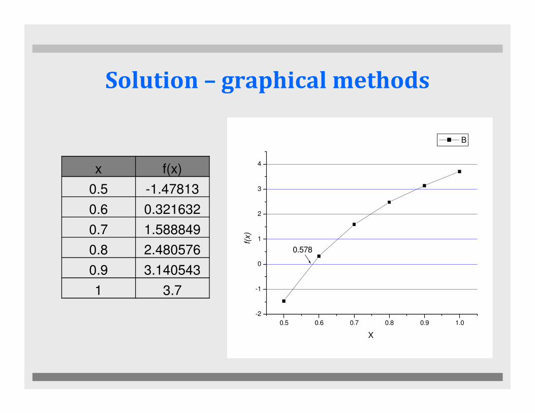
Solution – graphical methods

3

4

B

x f(x)

0.5 -1.47813

0.6 0.321632

0.5 0.6 0.7 0.8 0.9 1.0

-2

-1

0

1

2

0.578f(

x)

X

0.6 0.321632

0.7 1.588849

0.8 2.480576

0.9 3.140543

1 3.7

CHAPTER 3bCHAPTER 3b

OPEN METHOD

Open methods – a)Simple fixed point iteration

� Re-arranging the function f(x)=0, so that x is one the left side of the

equation, i.e.

x=g(x) -------- 6.1

� Transformation can be accomplished either by algebraic manipulation

or by simply adding x to both sides of the original equation.or by simply adding x to both sides of the original equation.

e.g.

can be simply manipulated to yield

e.g. sin x = 0

By adding x to both sides to yield x = sin x + x

2 2 3 0x x− + =2 3

2

xx

+=

• Equation 6.1 provides formula to predict new value of x as

a function of an old value of x. Thus, given initial guess at

the root xi, to compute new estimate xi+1 as expressed by

the iterative formula;

------- 6.2( )x x g x⇒ = ------- 6.2

• Error estimator:

1 1 ( )i i ix x g x+ +⇒ =

1

1

100%i ia

i

x x

xε +

+

−=

Example 4

Use simple fixed-point iteration to locate

the root of f(x) = e-x – x. Given true value of

the root = 0.56714329the root = 0.56714329

Solution

when f(x) = 0, x = e-x

xi+1 = e-x starting with initial guess of x0 = 0

i xi Xi + 1 = e-x εεεεa(%) εεεεt(%)

0 0 0 - 100.0

1 0 1 100.0 76.3

2 1 0.367879 171.8 35.1

3 0.367879 0.692201 46.9 22.1

4 0.692201 38.3 11.8

%100367879.0

1367879.0 −=

aε

Solution

i xi εεεεa(%) εεεεt(%)

0 0 - 100.0

1 1.000000 100.0 76.3

2 0.367879 171.8 35.1

3 0.692201 46.9 22.13 0.692201 46.9 22.1

4 0.500473 38.3 11.8

5 0.606244 17.4 6.89

6 0.545396 11.2 3.83

7 0.579612 5.90 2.20

8 0.560115 3.48 1.24

9 0.571143 1.93 0.705

10 0.564879 1.11 0.399

b) Newton-Raphson Method• The most widely used of all root-locating formulas. In

this method, if the initial guess at the root is xi, a tangent

can be extended from the point [xi , f(xi)].

• The point where this tangent crosses the x axis usually

represents an improved estimate of the root.

• Based on Taylor series expansion;

• Rearrange to yield Newton-Raphson formula

----- 6.6

1

0)()(

+−−

=′ii

i

ixx

xfxf

x i + 1 = x i −f ( x i )

′ f ( x i )

Newton-Raphson• A convenient method for functions whose derivatives can be evaluated

analytically. Figure 6.5, pg 139 shows graphical depiction of the

Newton-Raphson method.

A tangent i.e. f ’(xi) is

extrapolated down to

x axis to provide an

estimate of the root at estimate of the root at

xi+1

Example 5

Use Newton-Raphson method to locate the root of

f(x) = e-x – x, f(x) = 0.

Given true value of the root = 0.56714329

Solution

The first derivative of the function can be

evaluated as:

f ’(x) = e-x -1

( )f x= −Substitute into NR formula:

Start the iteration with x0 = 0

1

1

( )

'( )

1

i

i

ii i

i

x

ii i x

f xx x

f x

e xx x

e

+

−

+ −

= −

−= −

− −

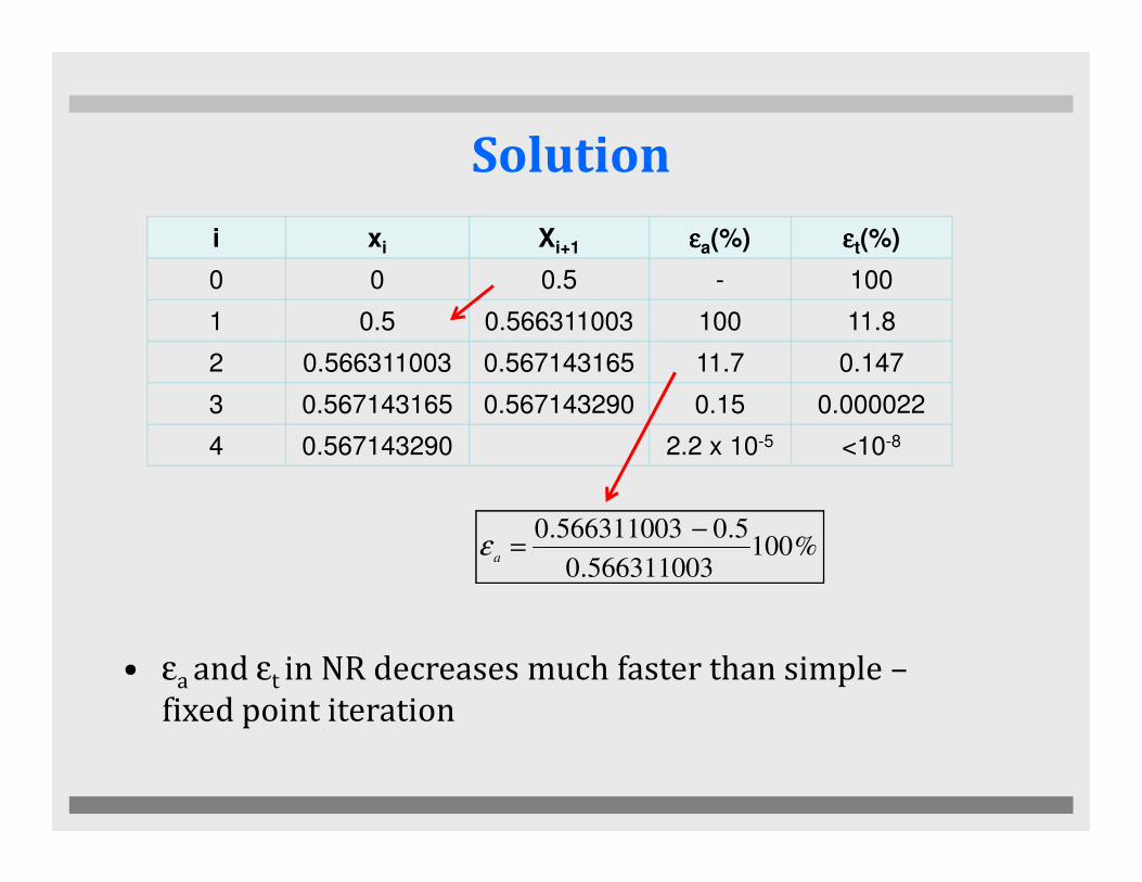
Solution

i xi Xi+1 εεεεa(%) εεεεt(%)

0 0 0.5 - 100

1 0.5 0.566311003 100 11.8

2 0.566311003 0.567143165 11.7 0.147

3 0.567143165 0.567143290 0.15 0.000022

4 0.567143290 2.2 x 10-5 <10-84 0.567143290 2.2 x 10-5 <10-8

• εa and εt in NR decreases much faster than simple –

fixed point iteration

%100566311003.0

5.0566311003.0 −=

aε

c) The Secant Method

• If derivatives extremely difficult or inconvenient to evaluate, “the secant

method” is used.

• The derivatives can be approximated by a backward finite divided

difference

• The technique is similar to NR (estimate of the root is predicted by

1

1

( ) ( )'( ) i i

i

i i

f x f xf x

x x

−

−

−=

−

• The technique is similar to NR (estimate of the root is predicted by

extrapolating a tangent of the function to x-axis), but the secant method

uses a difference, while NR uses derivative to estimate the slope (figure

6.7, pg 145).

• Substitute will

yield;

----- 6.7

11

1

( ) ( ) ( )'( ) in

'( )

i i ii i i

i i i

f x f x f xf x x x

x x f x

−+

−

−= = −

−

x i + 1 = x i −f ( x i ).( x i− 1 − x i )

f ( x i− 1 ) − f ( x i )

• Equation 6.7 is called a secant method. This approach requires twoinitial estimates of x. However, f(x) is not required to change signsbetween the estimates and hence it is not classified as a bracketingmethod.

f(x)

xixi+1

f(xi )

0

f(xi-1 )

x

Example 6

Use the secant method to estimate the root of

f(x) = e-x – x, f(x) = 0. Given true value of the root

= 0.56714329. Start with initial estimate of xi-1 == 0.56714329. Start with initial estimate of xi-1 =

0 and x0 = 1.0

Solution

1 1

0 0

1

1st iteration 0 ( ) 1

1.0 ( ) 0.63212

0.63212(0 1) 1 0.61270

1 ( 0.63212)

i ix f x

x f x

x

− −= =

= = −

− −= − =

− −

t

1 ( 0.63212)

0.56714329 0.61270 100% 8.03%

0.56714329ε

− −

−= =

Solution

0 0

1 1

1

t

2nd iteration 0 ( ) 0.63212

0.6127 ( ) 0.0708

0.07081(1 0.61270) 0.6127 0.56384

0.63212 ( 0.07081)

0.56714329 0.

x f x

x f x

x

ε

= = −

= = −

− −= − =

− − −

−=

56384100% 0.58%

0.56714329=t

0.56714329

1 1

2 2

1

t

3rd iteration 0.61270 ( ) 0.0708

0.56384 ( ) 0.00518

0.00518(0.61270 0.56384) 0.56384 0.56717

0.07081 ( 0.00518)

0

x f x

x f x

x

ε

= = −

= =

−= − =

− − −

=.56714329 0.56717

100% 0.0048%0.56714329

−=

Work with your buddy and

do Quiz 6 & Quiz 7

Comparison

Bracketing Methods Open Methods

� 2 initial guesses

� Root is located within lower and

upper interval, repeating will

result in closer estimates of true

value of the root

� 1 initial guess (Simple Fixed point

iteration and Newton –Raphson

method ) or 2 initial guesses

(Secant Method)

� not necessary bracket the rootvalue of the root

� Convergent due to it move closer to

the true value as the computation

progress

� not necessary bracket the root

� Sometimes diverge /move away

from the true root as computation

progress

� but if converge (closer to true

value) more quickly than

bracketing method.

Question?

THE END

Thank You for the Attention