Chapter 3Chapter 3

Molecular WeightMolecular Weight

1. Thermodynamics of Polymer Solution2. Mol Wt Determination

Ch 3-1 Slide 2

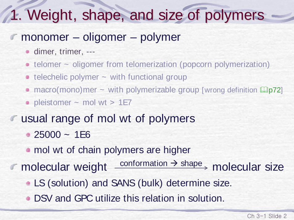
1. Weight, shape, and size of polymers1. Weight, shape, and size of polymersmonomer – oligomer – polymer

dimer, trimer, ---

telomer ~ oligomer from telomerization (popcorn polymerization)

telechelic polymer ~ with functional group

macro(mono)mer ~ with polymerizable group [wrong definition p72]

pleistomer ~ mol wt > 1E7

usual range of mol wt of polymers25000 ~ 1E6

mol wt of chain polymers are higher

molecular weight molecular sizeLS (solution) and SANS (bulk) determine size.

DSV and GPC utilize this relation in solution.

conformation shape

Ch 3-1 Slide 3

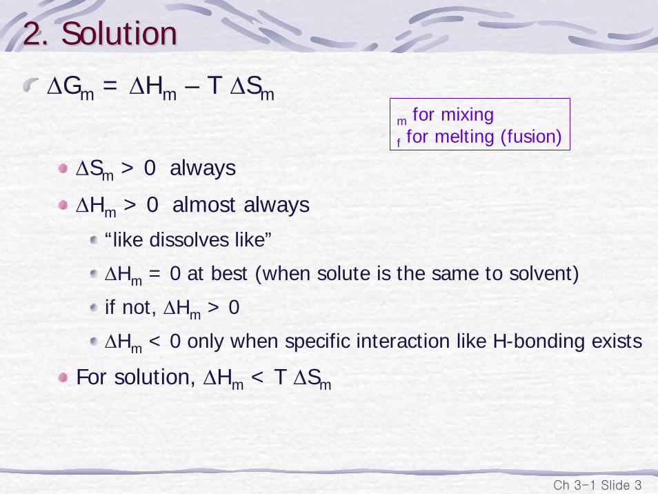
2. Solution2. SolutionΔGm = ΔHm – T ΔSm

ΔSm > 0 always

ΔHm > 0 almost always

“like dissolves like”

ΔHm = 0 at best (when solute is the same to solvent)

if not, ΔHm > 0

ΔHm < 0 only when specific interaction like H-bonding exists

For solution, ΔHm < T ΔSm

m for mixingf for melting (fusion)

Ch 3-1 Slide 4

Solubility parameterSolubility parameter

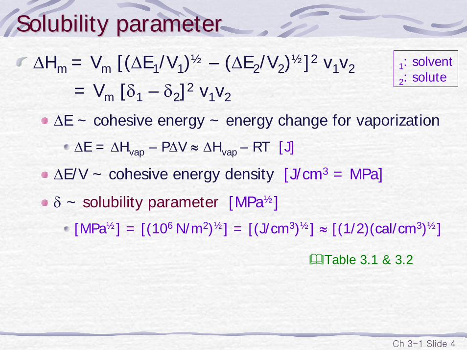
ΔHm = Vm [(ΔE1/V1)½ – (ΔE2/V2)½]2 v1v2

= Vm [δ1 – δ2]2 v1v2

ΔE ~ cohesive energy ~ energy change for vaporization

ΔE = ΔHvap – PΔV ≈ ΔHvap – RT [J]

ΔE/V ~ cohesive energy density [J/cm3 = MPa]

δ ~ solubility parameter [MPa½]

[MPa½] = [(106 N/m2)½] = [(J/cm3)½] ≈ [(1/2)(cal/cm3)½]

1: solvent2: solute

Table 3.1 & 3.2

Ch 3-1 Slide 5

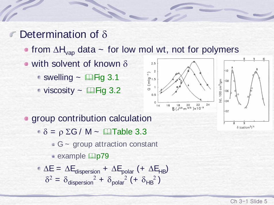
Determination of δfrom ΔHvap data ~ for low mol wt, not for polymers

with solvent of known δswelling ~ Fig 3.1

viscosity ~ Fig 3.2

group contribution calculationδ = ρ ΣG / M ~ Table 3.3

G ~ group attraction constant

example p79

ΔE = ΔEdispersion + ΔEpolar (+ ΔEHB)δ2 = δdispersion

2 + δpolar2 (+ δHB

2 )

Ch 3-1 Slide 6

For solution,ΔHm < T ΔSm

without specific interaction

δ1 = δ2 at best ΔHm = 0 ΔGm < 0

Δδ < 20 MPa½ (?) ~ for solvent/solvent solution

Δδ < 2 MPa½ ~ a rough guide for solvent/polymer solutionΔSm smaller

Δδ < 0.1 MPa½ ~ for polymer/polymer solution

semicrystalline polymers not soluble at RTpositive ΔHf ΔHf + ΔHm > T ΔSm

Table 3.2 ~ δ for amorphous state at 25 °C

Ch 3-1 Slide 7

3. Thermodynamics of polymer solution3. Thermodynamics of polymer solutionTypes of solutions

ideal soln ΔHm = 0, ΔSm = – k (N1 ln n1 + N2 ln n2)

regular soln ΔHm ≠ 0, ΔSm = – k (N1 ln n1 + N2 ln n2)

athermal soln ΔHm = 0, ΔSm ≠ – k (N1 ln n1 + N2 ln n2)

real soln

ideal solutionΔG1 = μ1 – μ1

o = RT ln n1

ΔG2 = μ2 – μ2o = RT ln n2

ΔGm = (N1/NA)ΔG1 + (N2/NA)ΔG2

= kT (N1 ln n1 + N2 ln n2)

ΔHm = 0 ΔSm = – k (N1 ln n1 + N2 ln n2)

Eqn (3.9) corrected

n: mol fractionN: number of moleculesn1 = N1/(N1+N2)

Eqn (3.12)

Ch 3-1 Slide 8

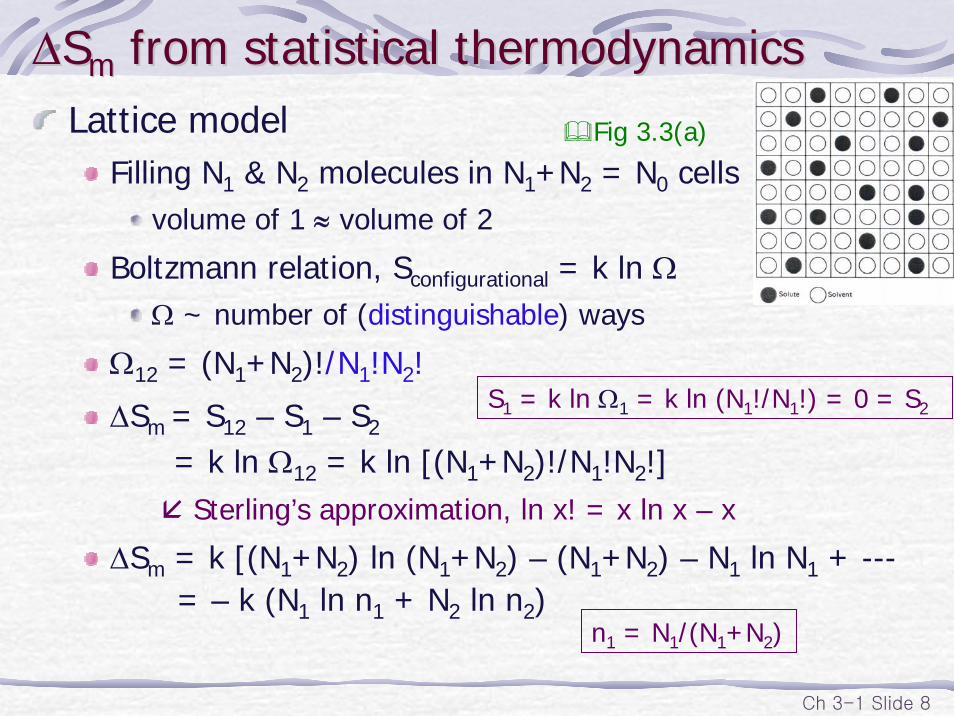
ΔΔSSmm from statistical thermodynamicsfrom statistical thermodynamicsLattice model

Filling N1 & N2 molecules in N1+N2 = N0 cellsvolume of 1 ≈ volume of 2

Boltzmann relation, Sconfigurational = k ln ΩΩ ~ number of (distinguishable) ways

Ω12 = (N1+N2)!/N1!N2!

ΔSm = S12 – S1 – S2

= k ln Ω12 = k ln [(N1+N2)!/N1!N2!]Sterling’s approximation, ln x! = x ln x – x

ΔSm = k [(N1+N2) ln (N1+N2) – (N1+N2) – N1 ln N1 + ---= – k (N1 ln n1 + N2 ln n2)

Fig 3.3(a)

S1 = k ln Ω1 = k ln (N1!/N1!) = 0 = S2

n1 = N1/(N1+N2)

Ch 3-1 Slide 9

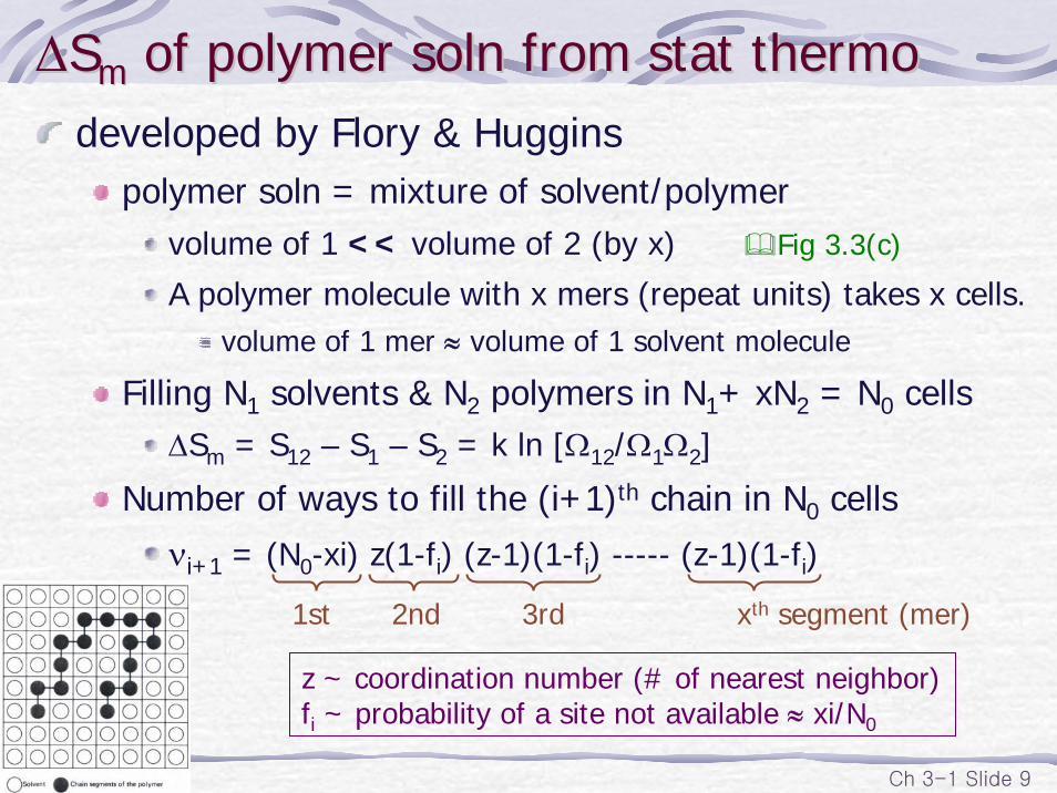
ΔΔSSmm of polymer of polymer solnsoln from stat thermofrom stat thermodeveloped by Flory & Huggins

polymer soln = mixture of solvent/polymervolume of 1 << volume of 2 (by x)

A polymer molecule with x mers (repeat units) takes x cells.volume of 1 mer ≈ volume of 1 solvent molecule

Filling N1 solvents & N2 polymers in N1+ xN2 = N0 cellsΔSm = S12 – S1 – S2 = k ln [Ω12/Ω1Ω2]

Number of ways to fill the (i+1)th chain in N0 cells

νi+1 = (N0-xi) z(1-fi) (z-1)(1-fi) ----- (z-1)(1-fi)

1st 2nd 3rd xth segment (mer)

z ~ coordination number (# of nearest neighbor)fi ~ probability of a site not available ≈ xi/N0

Fig 3.3(c)

Ch 3-1 Slide 10

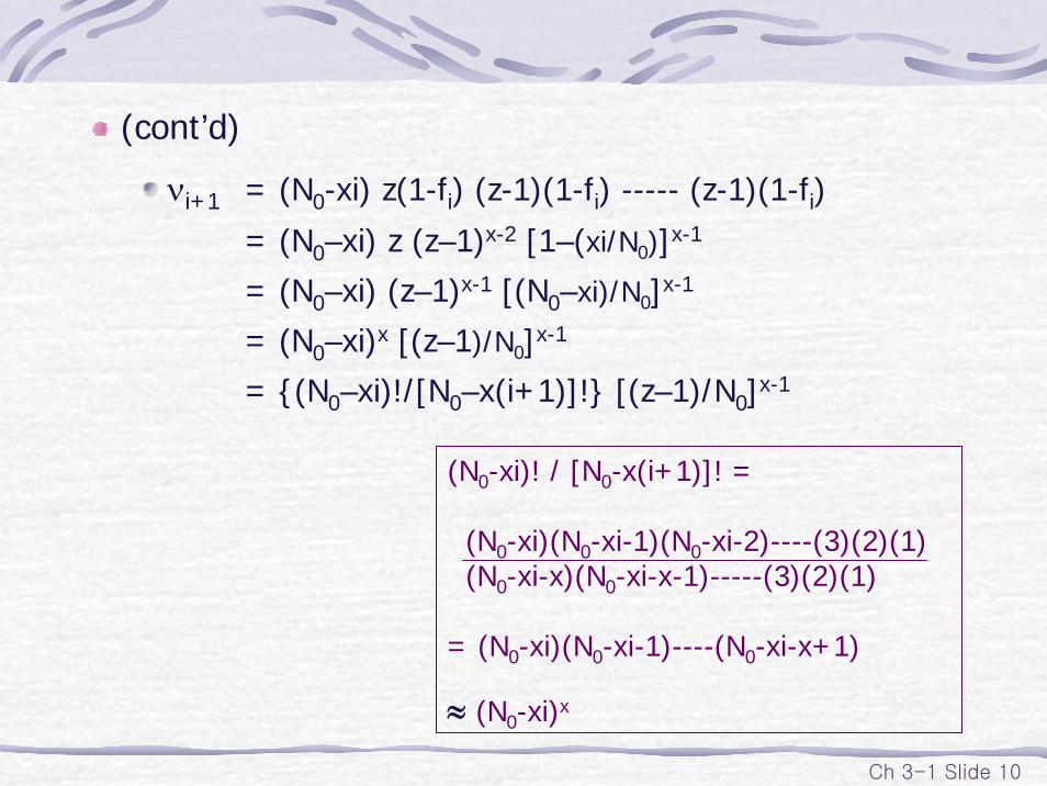
(cont’d)

νi+1 = (N0-xi) z(1-fi) (z-1)(1-fi) ----- (z-1)(1-fi)

= (N0–xi) z (z–1)x-2 [1–(xi/N0)]x-1

= (N0–xi) (z–1)x-1 [(N0–xi)/N0]x-1

= (N0–xi)x [(z–1)/N0]x-1

= {(N0–xi)!/[N0–x(i+1)]!} [(z–1)/N0]x-1

(N0-xi)! / [N0-x(i+1)]! =

(N0-xi)(N0-xi-1)(N0-xi-2)----(3)(2)(1)(N0-xi-x)(N0-xi-x-1)-----(3)(2)(1)

= (N0-xi)(N0-xi-1)----(N0-xi-x+1)

≈ (N0-xi)x

Ch 3-1 Slide 11

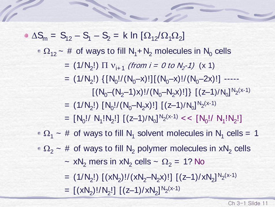
ΔSm = S12 – S1 – S2 = k ln [Ω12/Ω1Ω2]

Ω12 ~ # of ways to fill N1+N2 molecules in N0 cells

= (1/N2!) Π νi+1 (from i = 0 to N2-1) (x 1)

= (1/N2!) {[N0!/(N0–x)!][(N0–x)!/(N0–2x)!] -----

[(N0–(N2–1)x)!/(N0–N2x)!]} [(z–1)/N0]N2(x-1)

= (1/N2!) [N0!/(N0–N2x)!] [(z–1)/N0]N2(x-1)

= [N0!/ N1!N2!] [(z–1)/N0]N2(x-1) << [N0!/ N1!N2!]

Ω1 ~ # of ways to fill N1 solvent molecules in N1 cells = 1

Ω2 ~ # of ways to fill N2 polymer molecules in xN2 cells

~ xN2 mers in xN2 cells ~ Ω2 = 1? No

= (1/N2!) [(xN2)!/(xN2–N2x)!] [(z–1)/xN2]N2(x-1)

= [(xN2)!/N2!] [(z–1)/xN2]N2(x-1)

Ch 3-1 Slide 12

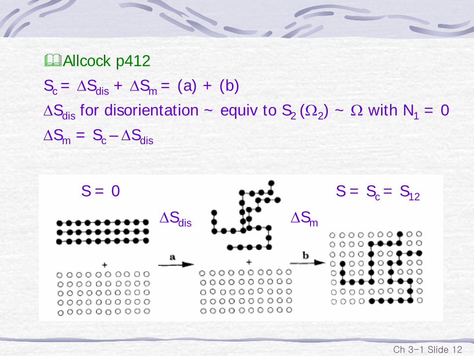
Allcock p412

Sc = ΔSdis + ΔSm = (a) + (b)

ΔSdis for disorientation ~ equiv to S2 (Ω2) ~ Ω with N1 = 0

ΔSm = Sc – ΔSdis

ΔSmΔSdis

S = 0 S = Sc = S12

Ch 3-1 Slide 13

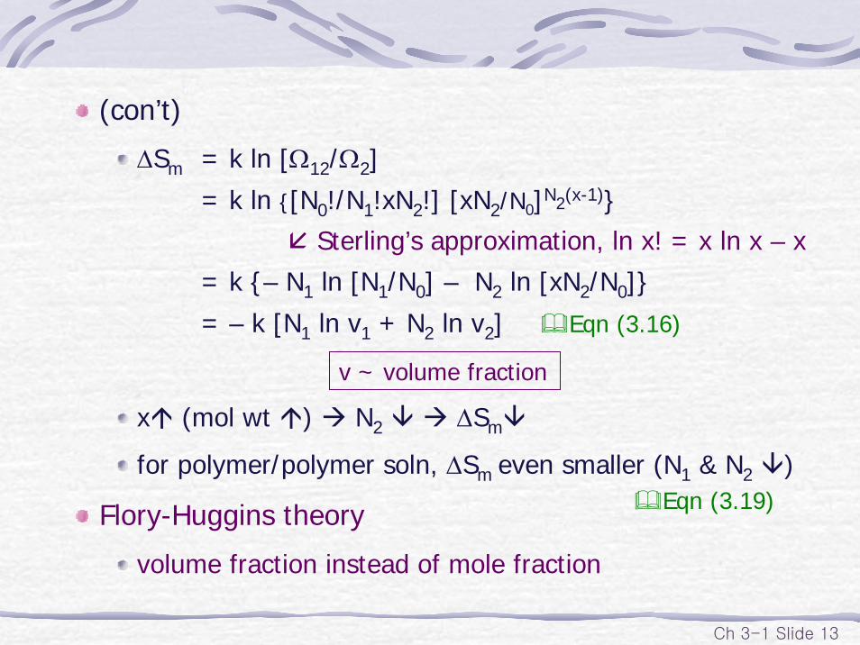
(con’t)

ΔSm = k ln [Ω12/Ω2]

= k ln {[N0!/N1!xN2!] [xN2/N0]N2(x-1)}Sterling’s approximation, ln x! = x ln x – x

= k {– N1 ln [N1/N0] – N2 ln [xN2/N0]}

= – k [N1 ln v1 + N2 ln v2]

x (mol wt ) N2 ΔSm

for polymer/polymer soln, ΔSm even smaller (N1 & N2 )

Flory-Huggins theory

volume fraction instead of mole fraction

Eqn (3.16)

v ~ volume fraction

Eqn (3.19)

Ch 3-1 Slide 14

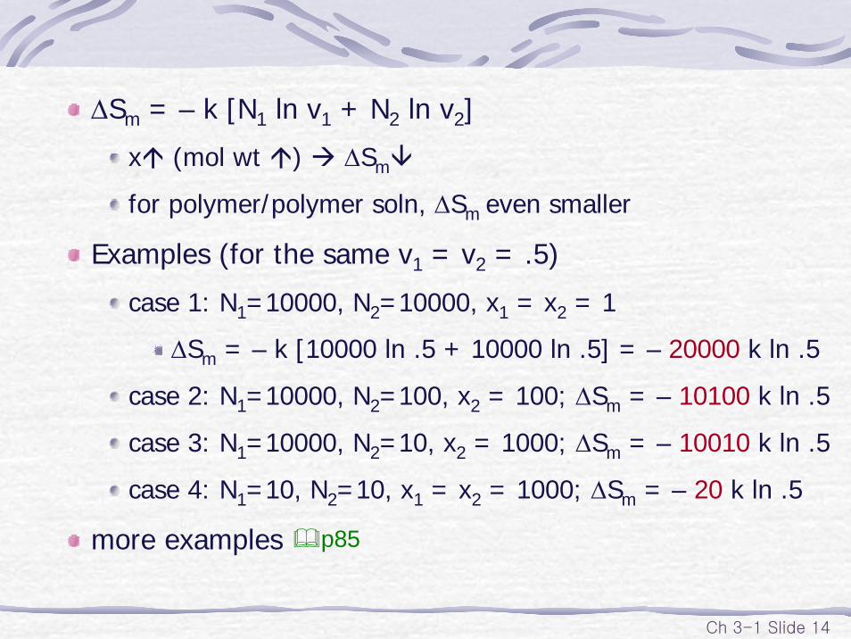
ΔSm = – k [N1 ln v1 + N2 ln v2]

x (mol wt ) ΔSm

for polymer/polymer soln, ΔSm even smaller

Examples (for the same v1 = v2 = .5)

case 1: N1=10000, N2=10000, x1 = x2 = 1

ΔSm = – k [10000 ln .5 + 10000 ln .5] = – 20000 k ln .5

case 2: N1=10000, N2=100, x2 = 100; ΔSm = – 10100 k ln .5

case 3: N1=10000, N2=10, x2 = 1000; ΔSm = – 10010 k ln .5

case 4: N1=10, N2=10, x1 = x2 = 1000; ΔSm = – 20 k ln .5

more examples p85

Ch 3-1 Slide 15

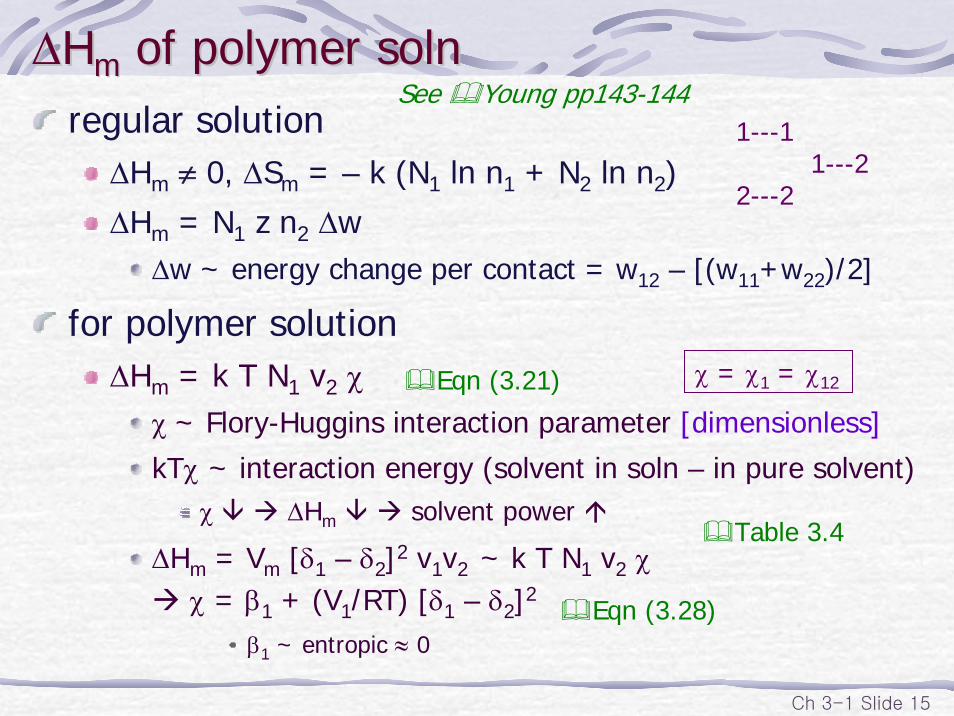
ΔΔHHmm of polymer of polymer solnsolnregular solution

ΔHm ≠ 0, ΔSm = – k (N1 ln n1 + N2 ln n2)

ΔHm = N1 z n2 ΔwΔw ~ energy change per contact = w12 – [(w11+w22)/2]

for polymer solutionΔHm = k T N1 v2 χ

χ ~ Flory-Huggins interaction parameter [dimensionless]

kTχ ~ interaction energy (solvent in soln – in pure solvent)χ ΔHm solvent power

ΔHm = Vm [δ1 – δ2]2 v1v2 ~ k T N1 v2 χχ = β1 + (V1/RT) [δ1 – δ2]2

β1 ~ entropic ≈ 0

χ = χ1 = χ12Eqn (3.21)

Table 3.4

Eqn (3.28)

1---11---2

2---2

See Young pp143-144

Ch 3-1 Slide 16

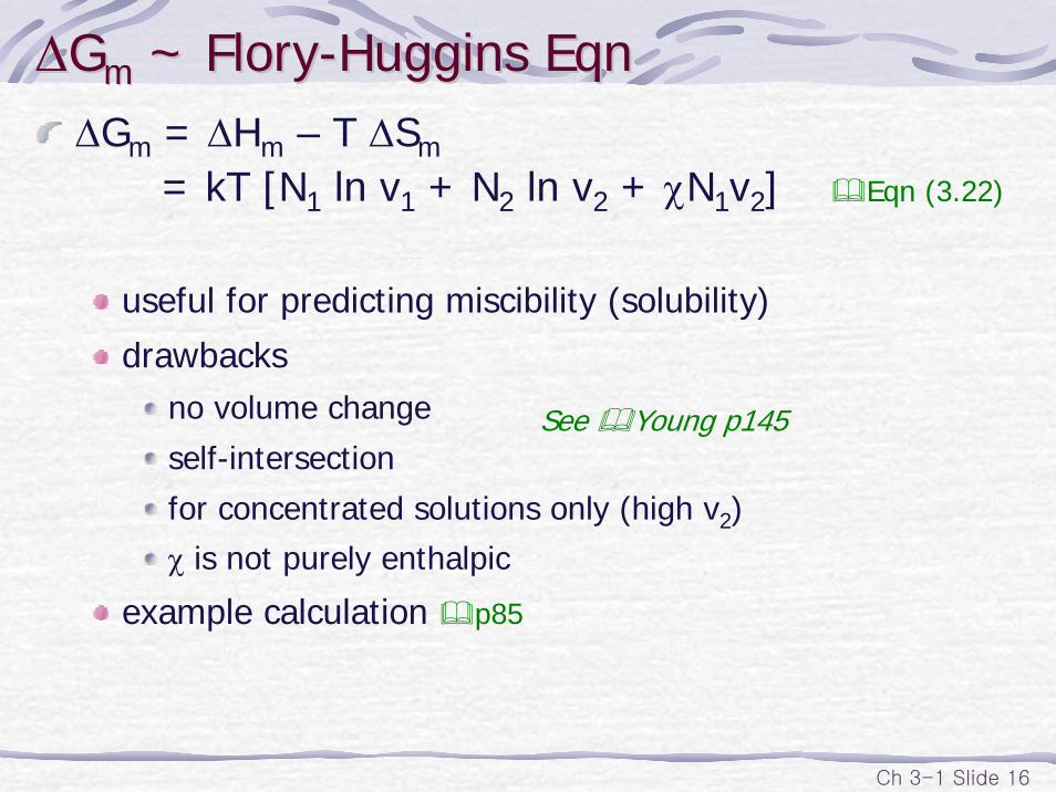
ΔΔGGmm ~ Flory~ Flory--Huggins Huggins EqnEqnΔGm = ΔHm – T ΔSm

= kT [N1 ln v1 + N2 ln v2 + χN1v2]

useful for predicting miscibility (solubility)

drawbacksno volume change

self-intersection

for concentrated solutions only (high v2)χ is not purely enthalpic

example calculation p85

Eqn (3.22)

See Young p145

Ch 3-1 Slide 17

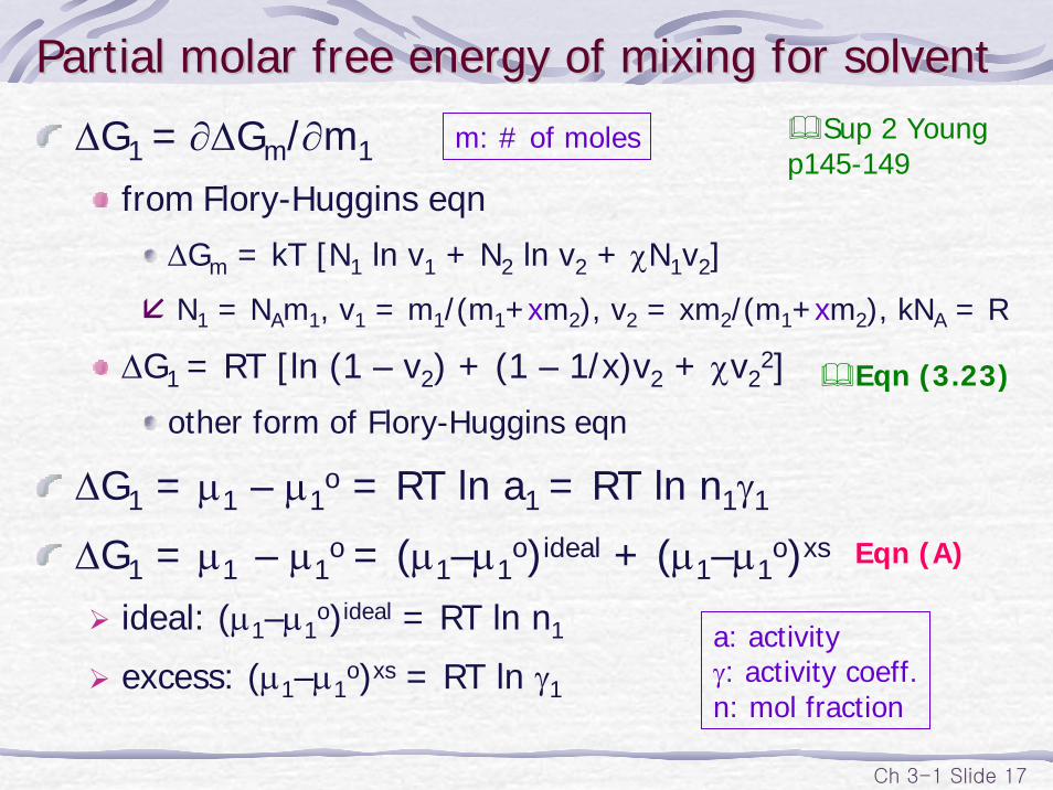
Partial molar free energy of mixing for solventPartial molar free energy of mixing for solvent

ΔG1 = ∂ΔGm/∂m1

from Flory-Huggins eqn

ΔGm = kT [N1 ln v1 + N2 ln v2 + χN1v2]

N1 = NAm1, v1 = m1/(m1+xm2), v2 = xm2/(m1+xm2), kNA = R

ΔG1 = RT [ln (1 – v2) + (1 – 1/x)v2 + χv22]

other form of Flory-Huggins eqn

ΔG1 = μ1 – μ1o = RT ln a1 = RT ln n1γ1

ΔG1 = μ1 – μ1o = (μ1–μ1

o)ideal + (μ1–μ1o)xs

ideal: (μ1–μ1o)ideal = RT ln n1

excess: (μ1–μ1o)xs = RT ln γ1

m: # of moles

Eqn (3.23)

a: activityγ: activity coeff.n: mol fraction

Eqn (A)

Sup 2 Young p145-149

Ch 3-1 Slide 18

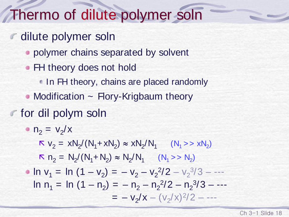
Thermo of Thermo of dilutedilute polymer polymer solnsolndilute polymer soln

polymer chains separated by solvent

FH theory does not holdIn FH theory, chains are placed randomly

Modification ~ Flory-Krigbaum theory

for dil polym solnn2 = v2/x

v2 = xN2/(N1+xN2) ≈ xN2/N1 (N1 >> xN2)

n2 = N2/(N1+N2) ≈ N2/N1 (N1 >> N2)

ln v1 = ln (1 – v2) = – v2 – v22/2 – v2

3/3 – ---ln n1 = ln (1 – n2) = – n2 – n2

2/2 – n23/3 – ---

= – v2/x – (v2/x)2/2 – ---

Ch 3-1 Slide 19

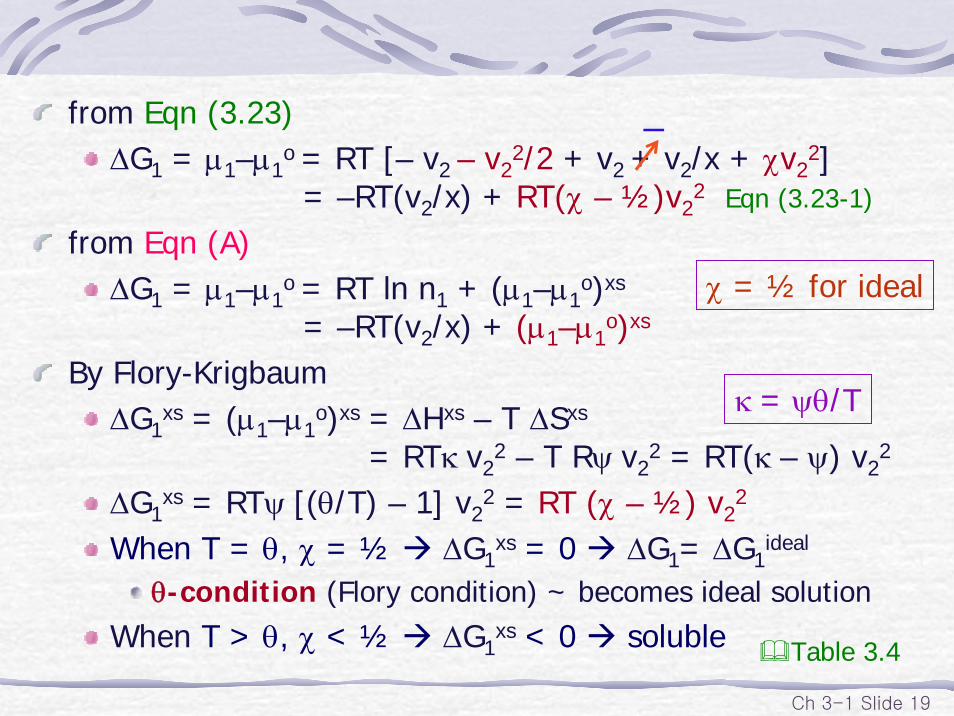
from Eqn (3.23)ΔG1 = μ1–μ1

o = RT [– v2 – v22/2 + v2 + v2/x + χv2

2]= –RT(v2/x) + RT(χ – ½)v2

2 Eqn (3.23-1)

from Eqn (A)ΔG1 = μ1–μ1

o = RT ln n1 + (μ1–μ1o)xs

= –RT(v2/x) + (μ1–μ1o)xs

By Flory-KrigbaumΔG1

xs = (μ1–μ1o)xs = ΔHxs – T ΔSxs

= RTκ v22 – T Rψ v2

2 = RT(κ – ψ) v22

ΔG1xs = RTψ [(θ/T) – 1] v2

2 = RT (χ – ½) v22

When T = θ, χ = ½ ΔG1xs = 0 ΔG1= ΔG1

ideal

θ-condition (Flory condition) ~ becomes ideal solutionWhen T > θ, χ < ½ ΔG1

xs < 0 soluble

κ = ψθ/T

Table 3.4

–

χ = ½ for ideal

Chapter 3Chapter 3

Molecular WeightMolecular Weight

1. Thermodynamics of Polymer Solution

2. Mol Wt Determination

Ch 3-1 Slide 21

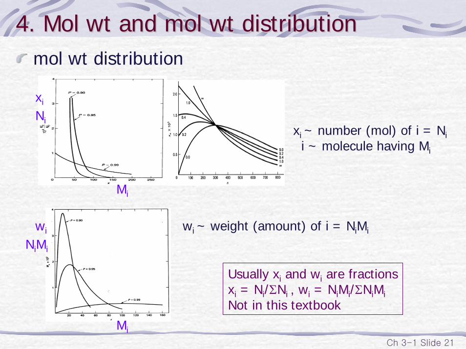
4. Mol wt and mol wt distribution4. Mol wt and mol wt distributionmol wt distribution

xi ~ number (mol) of i = Nii ~ molecule having Mi

wi ~ weight (amount) of i = NiMi

Usually xi and wi are fractionsxi = Ni/ΣNi , wi = NiMi/ΣNiMiNot in this textbook

Ni

xi

Mi

Mi

wi

NiMi

Ch 3-1 Slide 22

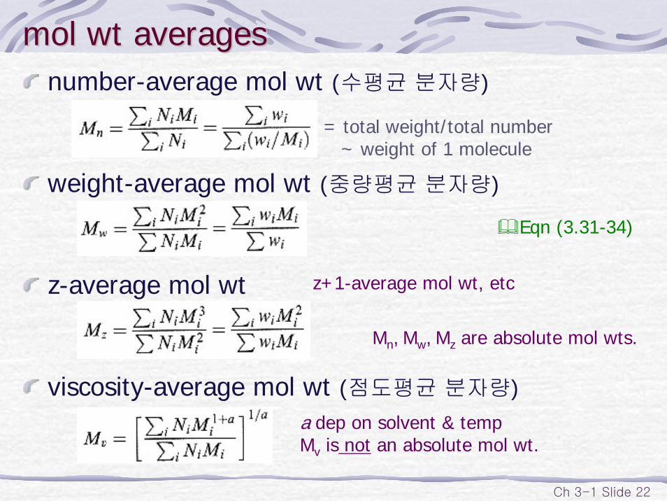
mol wt averagesmol wt averagesnumber-average mol wt (수평균 분자량)

weight-average mol wt (중량평균 분자량)

z-average mol wt

viscosity-average mol wt (점도평균 분자량)

= total weight/total number~ weight of 1 molecule

a dep on solvent & tempMv is not an absolute mol wt.

Mn, Mw, Mz are absolute mol wts.

z+1-average mol wt, etc

Eqn (3.31-34)

Ch 3-1 Slide 23

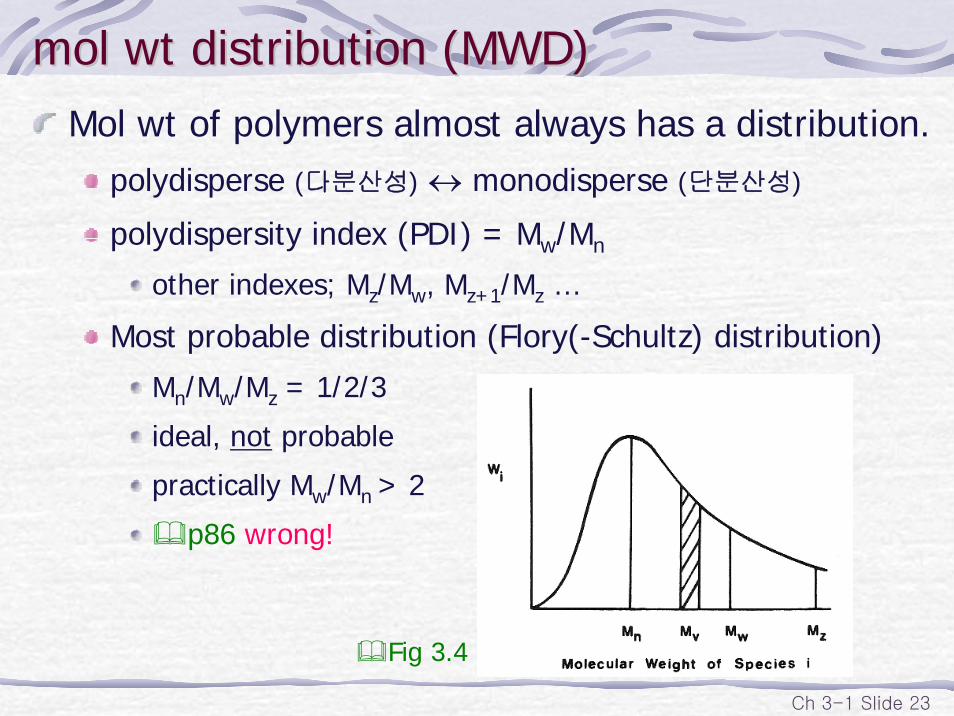
mol wt distribution (MWD)mol wt distribution (MWD)Mol wt of polymers almost always has a distribution.

polydisperse (다분산성) ↔ monodisperse (단분산성)

polydispersity index (PDI) = Mw/Mn

other indexes; Mz/Mw, Mz+1/Mz …

Most probable distribution (Flory(-Schultz) distribution)

Mn/Mw/Mz = 1/2/3

ideal, not probable

practically Mw/Mn > 2

p86 wrong!

Fig 3.4

Ch 3-1 Slide 24

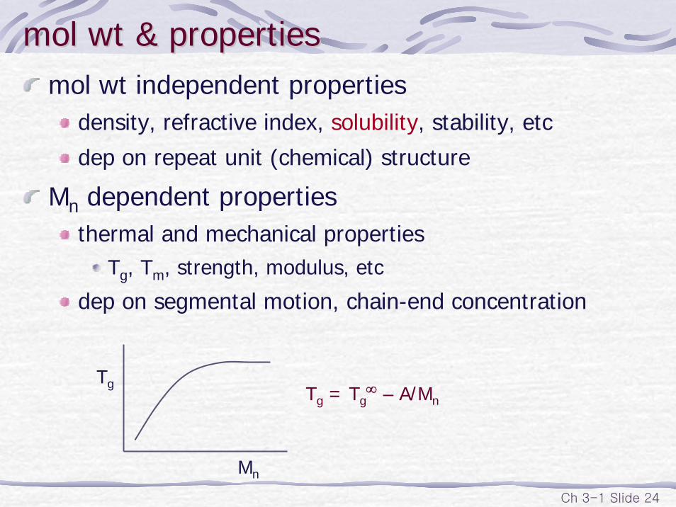
mol wt & propertiesmol wt & propertiesmol wt independent properties

density, refractive index, solubility, stability, etc

dep on repeat unit (chemical) structure

Mn dependent propertiesthermal and mechanical properties

Tg, Tm, strength, modulus, etc

dep on segmental motion, chain-end concentration

Tg = Tg∞ – A/Mn

Tg

Mn

Ch 3-1 Slide 25

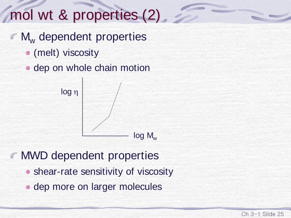
mol wt & properties (2)mol wt & properties (2)Mw dependent properties

(melt) viscosity

dep on whole chain motion

MWD dependent propertiesshear-rate sensitivity of viscosity

dep more on larger molecules

log η

log Mw

Ch 3-1 Slide 26

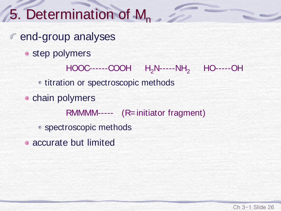
5. Determination of 5. Determination of MMnn

end-group analysesstep polymers

HOOC------COOH H2N-----NH2 HO-----OH

titration or spectroscopic methods

chain polymers

RMMMM----- (R=initiator fragment)

spectroscopic methods

accurate but limited

Ch 3-1 Slide 27

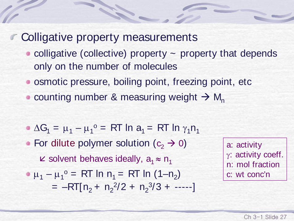
Colligative property measurementscolligative (collective) property ~ property that depends only on the number of molecules

osmotic pressure, boiling point, freezing point, etc

counting number & measuring weight Mn

ΔG1 = μ1 – μ1o = RT ln a1 = RT ln γ1n1

For dilute polymer solution (c2 0)

solvent behaves ideally, a1 ≈ n1

μ1 – μ1o = RT ln n1 = RT ln (1–n2)

= –RT[n2 + n22/2 + n2

3/3 + -----]

a: activityγ: activity coeff.n: mol fractionc: wt conc’n

Ch 3-1 Slide 28

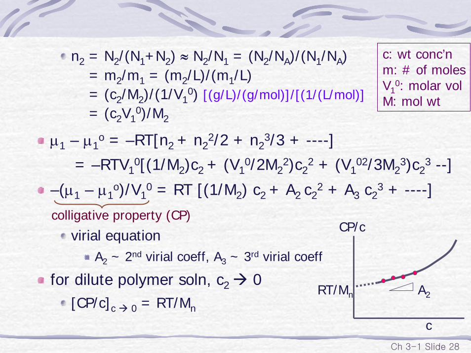
n2 = N2/(N1+N2) ≈ N2/N1 = (N2/NA)/(N1/NA) = m2/m1 = (m2/L)/(m1/L) = (c2/M2)/(1/V1

0) [(g/L)/(g/mol)]/[(1/(L/mol)]= (c2V1

0)/M2

μ1 – μ1o = –RT[n2 + n2

2/2 + n23/3 + ----]

= –RTV10[(1/M2)c2 + (V1

0/2M22)c2

2 + (V102/3M2

3)c23 --]

–(μ1 – μ1o)/V1

0 = RT [(1/M2) c2 + A2 c22 + A3 c2

3 + ----]

virial equationA2 ~ 2nd virial coeff, A3 ~ 3rd virial coeff

for dilute polymer soln, c2 0[CP/c]c 0 = RT/Mn

colligative property (CP)CP/c

c

A2RT/Mn

c: wt conc’nm: # of molesV1

0: molar volM: mol wt

Ch 3-1 Slide 29

ebulliometry (bp elevation)ΔTb/c = Ke [(1/Mn) + A2 c + A3 c2 + ----]

Ke calibrated with known mol wt

limited by precision of temperature measurementuseful only for Mn < 30000

not used these days

cryoscopy (fp depression)ΔTf/c = Kc [(1/Mn) + A2 c + A3 c2 + ----]

Kc calibrated with known mol wt

limited by precision of temperature measurementuseful only for Mn < 30000

not used these days

Eqn (3.35)

Eqn (3.36)

Ch 3-1 Slide 30

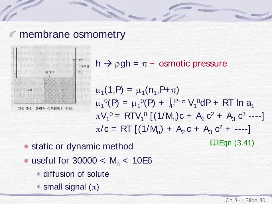
membrane osmometry

static or dynamic method

useful for 30000 < Mn < 10E6diffusion of solutesmall signal (π)

h ρgh = π ~ osmotic pressure

μ1(1,P) = μ1(n1,P+π) μ1

0(P) = μ10(P) + ∫PP+π V1

0dP + RT ln a1

πV10 = RTV1

0 [(1/Mn)c + A2 c2 + A3 c3 ----]π/c = RT [(1/Mn) + A2 c + A3 c2 + ----]

Eqn (3.41)

Ch 3-1 Slide 31

Determination without extrapolation?πV1

0 = RTV10 [(1/Mn)c+A2 c2+ --] = –RT ln a1 = –(μ1–μ1

o)

μ1–μ1o = –RT(v2/x) + RT(χ – ½)v2

2

π = RT(v2/xV10) + RT(χ – ½)v2

2/V10

v2 ≈ xN2/N1, V = (N1/NA)V10, Mn = ΣNiMi/ΣNi = M2/(N2/NA)

c2 = M2/V = MnN2/NAV, ρ2 = V2/Mn, x = V2/V1

π/c = RT(1/Mn) + RT (χ – ½)(1/V1ρ22) c

= RT [1/Mn + A2 c]At θ-condition, χ = ½ , A2 = 0

no conc’n dependence

determination at 1 conc’n ~ need no extrapolation

hard to do ~ not a good solvent (ppt)

Eqn (3.23-1) dil soln

Eqn (3.26)

Fig 3.5

Ch 3-1 Slide 32

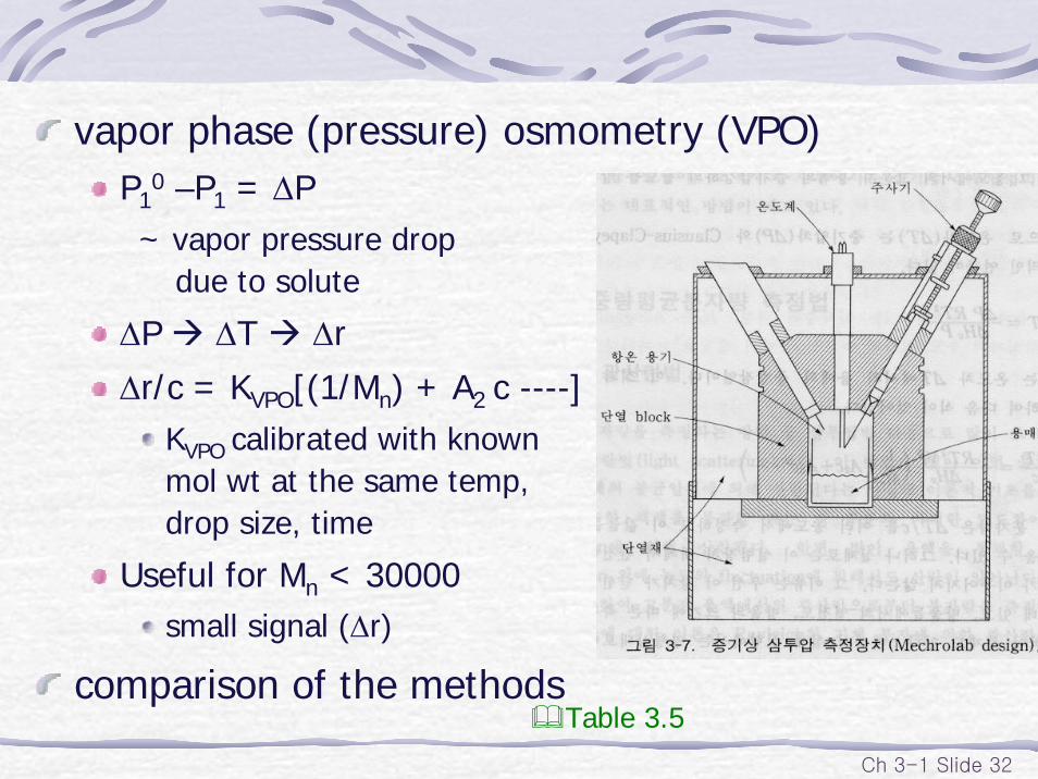
vapor phase (pressure) osmometry (VPO)P1

0 –P1 = ΔP~ vapor pressure drop

due to solute

ΔP ΔT Δr

Δr/c = KVPO[(1/Mn) + A2 c ----]KVPO calibrated with known mol wt at the same temp,drop size, time

Useful for Mn < 30000small signal (Δr)

comparison of the methods Table 3.5

Ch 3-1 Slide 33

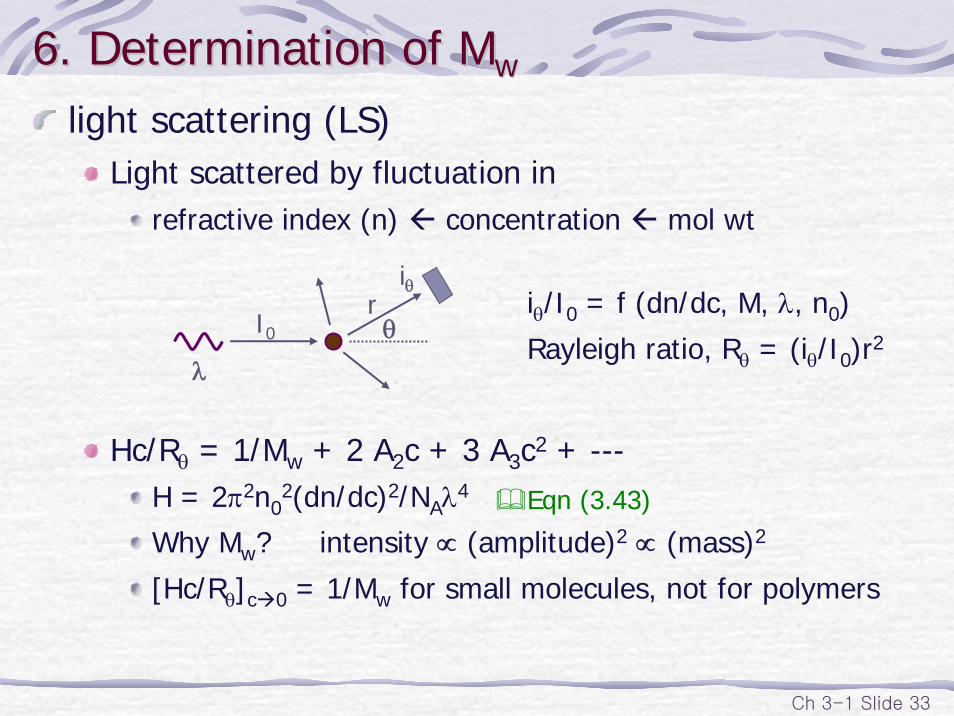
6. Determination of M6. Determination of Mww

light scattering (LS)Light scattered by fluctuation in

refractive index (n) concentration mol wt

Hc/Rθ = 1/Mw + 2 A2c + 3 A3c2 + ---H = 2π2n0

2(dn/dc)2/NAλ4

Why Mw? intensity ∝ (amplitude)2 ∝ (mass)2

[Hc/Rθ]c 0 = 1/Mw for small molecules, not for polymers

θr

I0

λ

iθiθ/I0 = f (dn/dc, M, λ, n0)

Rayleigh ratio, Rθ = (iθ/I0)r2

Eqn (3.43)

Ch 3-1 Slide 34

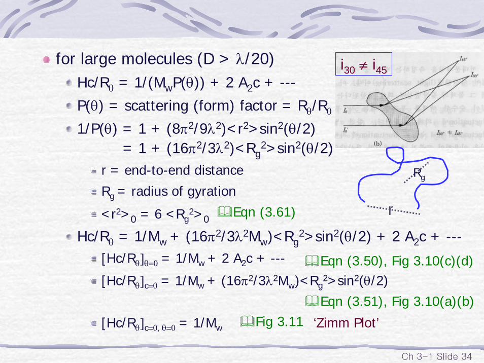
for large molecules (D > λ/20)Hc/Rθ = 1/(MwP(θ)) + 2 A2c + ---

P(θ) = scattering (form) factor = Rθ/R0

1/P(θ) = 1 + (8π2/9λ2)<r2>sin2(θ/2)= 1 + (16π2/3λ2)<Rg

2>sin2(θ/2)r = end-to-end distance

Rg = radius of gyration

<r2>0 = 6 <Rg2>0

Hc/Rθ = 1/Mw + (16π2/3λ2Mw)<Rg2>sin2(θ/2) + 2 A2c + ---

[Hc/Rθ]θ=0 = 1/Mw + 2 A2c + ---

[Hc/Rθ]c=0 = 1/Mw + (16π2/3λ2Mw)<Rg2>sin2(θ/2)

[Hc/Rθ]c=0, θ=0 = 1/Mw ‘Zimm Plot’

r

Rg

Eqn (3.50), Fig 3.10(c)(d)

i30 ≠ i45

Eqn (3.51), Fig 3.10(a)(b)Fig 3.11

Eqn (3.61)

Ch 3-1 Slide 35

7. MW of common polymers7. MW of common polymersMW of commercial polymers

step polymers: 20000 – 40000

chain polymers: 20000 – 1000000

MWDFlory-Schultz distribution: PDI = 2

when ideal

Poisson distribution: PDI = 1anionic living polymerization

In most polymerizations: PDI > 2Table 3.9

PDI(chain polymers) > PDI(step polymers)

Ch 3-1 Slide 36

8. Determination of 8. Determination of MMvv

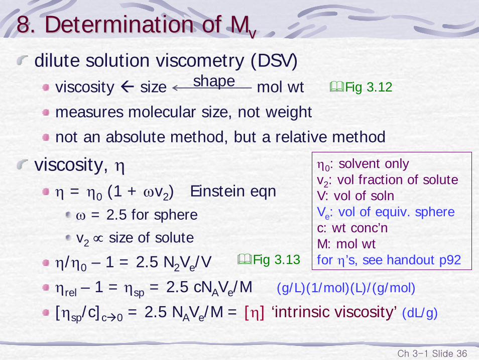
dilute solution viscometry (DSV)viscosity size mol wt

measures molecular size, not weight

not an absolute method, but a relative method

viscosity, ηη = η0 (1 + ωv2) Einstein eqn

ω = 2.5 for sphere

v2 ∝ size of solute

η/η0 – 1 = 2.5 N2Ve/V

ηrel – 1 = ηsp = 2.5 cNAVe/M (g/L)(1/mol)(L)/(g/mol)

[ηsp/c]c 0 = 2.5 NAVe/M = [η] ‘intrinsic viscosity’ (dL/g)

η0: solvent onlyv2: vol fraction of soluteV: vol of solnVe: vol of equiv. spherec: wt conc’nM: mol wtfor η’s, see handout p92Fig 3.13

Fig 3.12shape

Ch 3-1 Slide 37

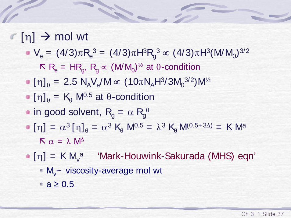
[η] mol wtVe = (4/3)πRe

3 = (4/3)πH3Rg3 ∝ (4/3)πH3(M/M0)3/2

Re = HRg, Rg ∝ (M/M0)½ at θ-condition

[η]θ = 2.5 NAVe/M ∝ (10πNAH3/3M03/2)M½

[η]θ = Kθ M0.5 at θ-condition

in good solvent, Rg = α Rgθ

[η] = α3 [η]θ = α3 Kθ M0.5 = λ3 Kθ M(0.5+3Δ) = K Ma

α = λ MΔ

[η] = K Mva ‘Mark-Houwink-Sakurada (MHS) eqn’

Mv~ viscosity-average mol wta ≥ 0.5

Ch 3-1 Slide 38

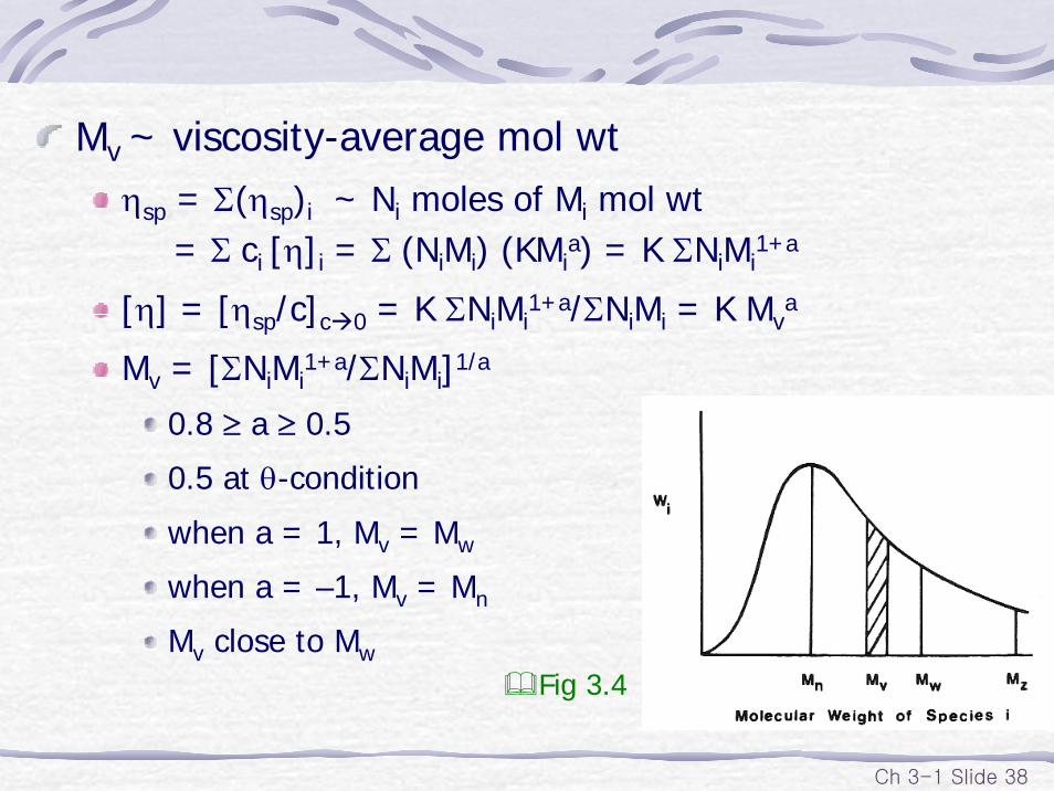
Mv ~ viscosity-average mol wtηsp = Σ(ηsp)i ~ Ni moles of Mi mol wt

= Σ ci [η]i = Σ (NiMi) (KMia) = K ΣNiMi

1+a

[η] = [ηsp/c]c 0 = K ΣNiMi1+a/ΣNiMi = K Mv

a

Mv = [ΣNiMi1+a/ΣNiMi]1/a

0.8 ≥ a ≥ 0.5

0.5 at θ-condition

when a = 1, Mv = Mw

when a = –1, Mv = Mn

Mv close to MwFig 3.4

Ch 3-1 Slide 39

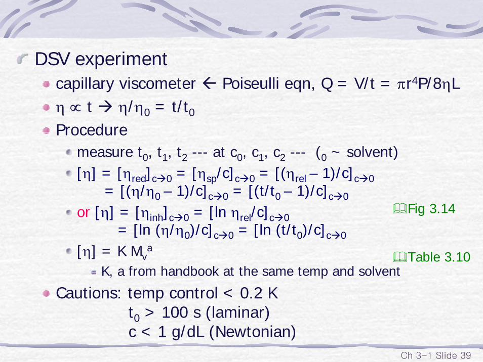
DSV experiment capillary viscometer Poiseulli eqn, Q = V/t = πr4P/8ηLη ∝ t η/η0 = t/t0Procedure

measure t0, t1, t2 --- at c0, c1, c2 --- (0 ~ solvent)[η] = [ηred]c 0 = [ηsp/c]c 0 = [(ηrel – 1)/c]c 0

= [(η/η0 – 1)/c]c 0 = [(t/t0 – 1)/c]c 0

or [η] = [ηinh]c 0 = [ln ηrel/c]c 0= [ln (η/η0)/c]c 0 = [ln (t/t0)/c]c 0

[η] = K Mva

K, a from handbook at the same temp and solvent

Cautions: temp control < 0.2 Kt0 > 100 s (laminar) c < 1 g/dL (Newtonian)

Table 3.10

Fig 3.14

Ch 3-1 Slide 40

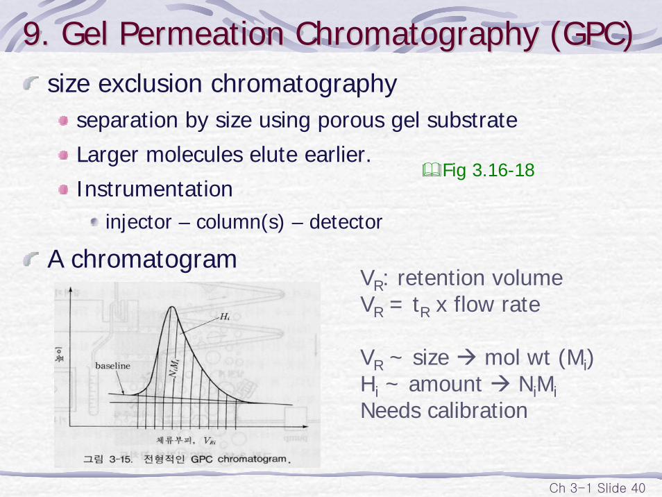
9. Gel Permeation Chromatography (GPC)9. Gel Permeation Chromatography (GPC)size exclusion chromatography

separation by size using porous gel substrate

Larger molecules elute earlier.

Instrumentationinjector – column(s) – detector

A chromatogram

Fig 3.16-18

VR: retention volumeVR = tR x flow rate

VR ~ size mol wt (Mi)Hi ~ amount NiMiNeeds calibration

Ch 3-1 Slide 41

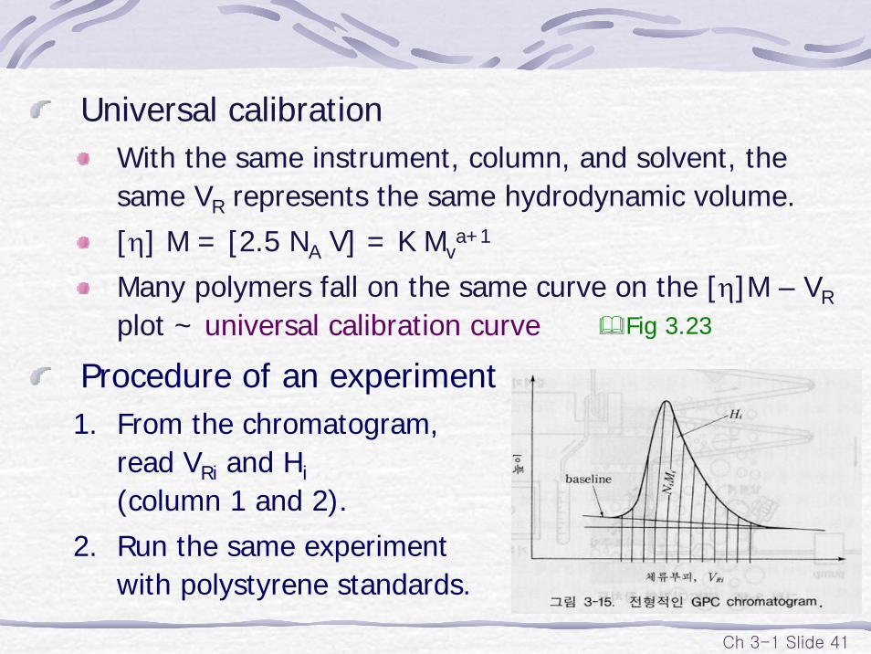
Universal calibrationWith the same instrument, column, and solvent, the same VR represents the same hydrodynamic volume.

[η] M = [2.5 NA V] = K Mva+1

Many polymers fall on the same curve on the [η]M – VR

plot ~ universal calibration curve

Procedure of an experiment1. From the chromatogram,

read VRi and Hi

(column 1 and 2).

2. Run the same experimentwith polystyrene standards.

Fig 3.23

Ch 3-1 Slide 42

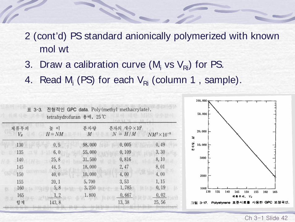
2 (cont’d) PS standard anionically polymerized with known mol wt

3. Draw a calibration curve (Mi vs VRi) for PS.

4. Read Mi (PS) for each VRi (column 1 , sample).

Ch 3-1 Slide 43

5. M (PS) M (sample)

[η]PSMPS = [η]sampleMsample

KPSMPSa(PS)+1 = KsampleMsample

a(sample)+1

6. Ni = Hi / Mi (column 2 / column 3)

7. Calculate Mn, Mw, MWD.

Are Mn and Mw obtained absolute? No.

from handbookfrom calibration curve

column 3

Ch 3-1 Slide 44

10. Mass spectrometry10. Mass spectrometryMS determines mol wt

by detecting molecular ion, M+

in vapor phase

ionization of polymers in gas phase?

MALDI-TOF techniquesoft ionization

choice of the matrix critical

for not-too-high mol wt

useful for (highly) branched polymers

Ch 3-1 Slide 45

11. Conclusions11. ConclusionsAt theta condition (solvent/temp)

A2 = 0, χ = ½

Rg is the same to that of the bulk polymer

infinite mol wt fraction just precipitate (poor/good)

Absolute and relative methodsTable 3.15