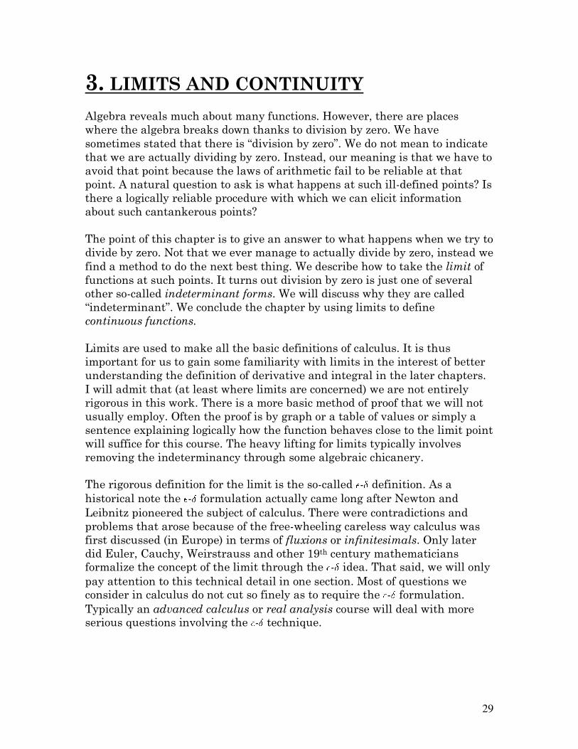
29

3. LIMITS AND CONTINUITY

Algebra reveals much about many functions. However, there are places

where the algebra breaks down thanks to division by zero. We have

sometimes stated that there is “division by zero”. We do not mean to indicate

that we are actually dividing by zero. Instead, our meaning is that we have to

avoid that point because the laws of arithmetic fail to be reliable at that

point. A natural question to ask is what happens at such ill-defined points? Is

there a logically reliable procedure with which we can elicit information

about such cantankerous points?

The point of this chapter is to give an answer to what happens when we try to

divide by zero. Not that we ever manage to actually divide by zero, instead we

find a method to do the next best thing. We describe how to take the limit of

functions at such points. It turns out division by zero is just one of several

other so-called indeterminant forms. We will discuss why they are called

“indeterminant”. We conclude the chapter by using limits to define

continuous functions.

Limits are used to make all the basic definitions of calculus. It is thus

important for us to gain some familiarity with limits in the interest of better

understanding the definition of derivative and integral in the later chapters.

I will admit that (at least where limits are concerned) we are not entirely

rigorous in this work. There is a more basic method of proof that we will not

usually employ. Often the proof is by graph or a table of values or simply a

sentence explaining logically how the function behaves close to the limit point

will suffice for this course. The heavy lifting for limits typically involves

removing the indeterminancy through some algebraic chicanery.

The rigorous definition for the limit is the so-called - definition. As a

historical note the - formulation actually came long after Newton and

Leibnitz pioneered the subject of calculus. There were contradictions and

problems that arose because of the free-wheeling careless way calculus was

first discussed (in Europe) in terms of fluxions or infinitesimals. Only later

did Euler, Cauchy, Weirstrauss and other 19th century mathematicians

formalize the concept of the limit through the - idea. That said, we will only

pay attention to this technical detail in one section. Most of questions we

consider in calculus do not cut so finely as to require the - formulation.

Typically an advanced calculus or real analysis course will deal with more

serious questions involving the - technique.

30

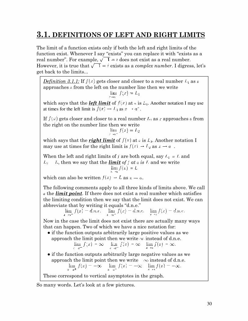
3.1. DEFINITIONS OF LEFT AND RIGHT LIMITS

The limit of a function exists only if both the left and right limits of the

function exist. Whenever I say “exists” you can replace it with “exists as a

real number”. For example, does not exist as a real number.

However, it is true that exists as a complex number. I digress, let’s

get back to the limits...

So many words. Let’s look at a few pictures.

Definition 3.1.1: If gets closer and closer to a real number as

approaches from the left on the number line then we write

which says that the left limit of at is . Another notation I may use

at times for the left limit is as .

If gets closer and closer to a real number as approaches from

the right on the number line then we write

which says that the right limit of at is . Another notation I

may use at times for the right limit is as .

When the left and right limits of are both equal, say and

, then we say that the limit of at is and we write

which can also be written as .

The following comments apply to all three kinds of limits above. We call

the limit point. If there does not exist a real number which satisfies

the limiting condition then we say that the limit does not exist. We can

abbreviate that by writing it equals “d.n.e.”

Now in the case the limit does not exist there are actually many ways

that can happen. Two of which we have a nice notation for:

● if the function outputs arbitrarily large positive values as we

approach the limit point then we write instead of d.n.e.

● if the function outputs arbitrarily large negative values as we

approach the limit point then we write instead of d.n.e.

These correspond to vertical asymptotes in the graph.

31

Let’s begin with a function with a hole in its graph. Suppose that the

following is the graph

We can easily see that as approaches 2 from the left or the right we get

closer and closer to 4. So we say that the . Notice that the limit

point is not in the domain of the function. That is pretty neat, we can

evaluate the limit at even though is undefined. For the function

pictured above we can see that for limit points other than we can

actually say that .

Next, let’s examine a function which has left and right limits at a particular

limit point, but they disagree. I’m tired of , let’s say the following is the

graph , let us examine the limit at

We see that as the function . On the other hand, as

we observe that . So the left limit is -2 while the right limit is 2. So

the one-sided limits exist but do not agree. Hence we say that the limit of

at zero does not exist. In other words, . I’ll grant you a

bonus point if you can give me an explicit formula for without breaking it

up into cases. (I know there is such a formula cause that’s how I graphed it.)

32

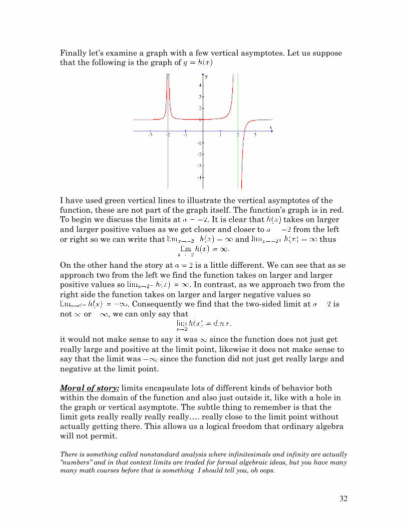
Finally let’s examine a graph with a few vertical asymptotes. Let us suppose

that the following is the graph of

I have used green vertical lines to illustrate the vertical asymptotes of the

function, these are not part of the graph itself. The function’s graph is in red.

To begin we discuss the limits at . It is clear that takes on larger

and larger positive values as we get closer and closer to from the left

or right so we can write that and thus

On the other hand the story at is a little different. We can see that as se

approach two from the left we find the function takes on larger and larger

positive values so . In contrast, as we approach two from the

right side the function takes on larger and larger negative values so

. Consequently we find that the two-sided limit at is

not or , we can only say that

it would not make sense to say it was since the function does not just get

really large and positive at the limit point, likewise it does not make sense to

say that the limit was since the function did not just get really large and

negative at the limit point.

Moral of story: limits encapsulate lots of different kinds of behavior both

within the domain of the function and also just outside it, like with a hole in

the graph or vertical asymptote. The subtle thing to remember is that the

limit gets really really really really…. really close to the limit point without

actually getting there. This allows us a logical freedom that ordinary algebra

will not permit.

There is something called nonstandard analysis where infinitesimals and infinity are actually

“numbers” and in that context limits are traded for formal algebraic ideas, but you have many

many math courses before that is something I should tell you, oh oops.

33

3.2. CONTINUOUS FUNCTIONS

Almost all the functions that arise in basic applications are continuous or

piecewise continuous (will discuss later). Without further ado,

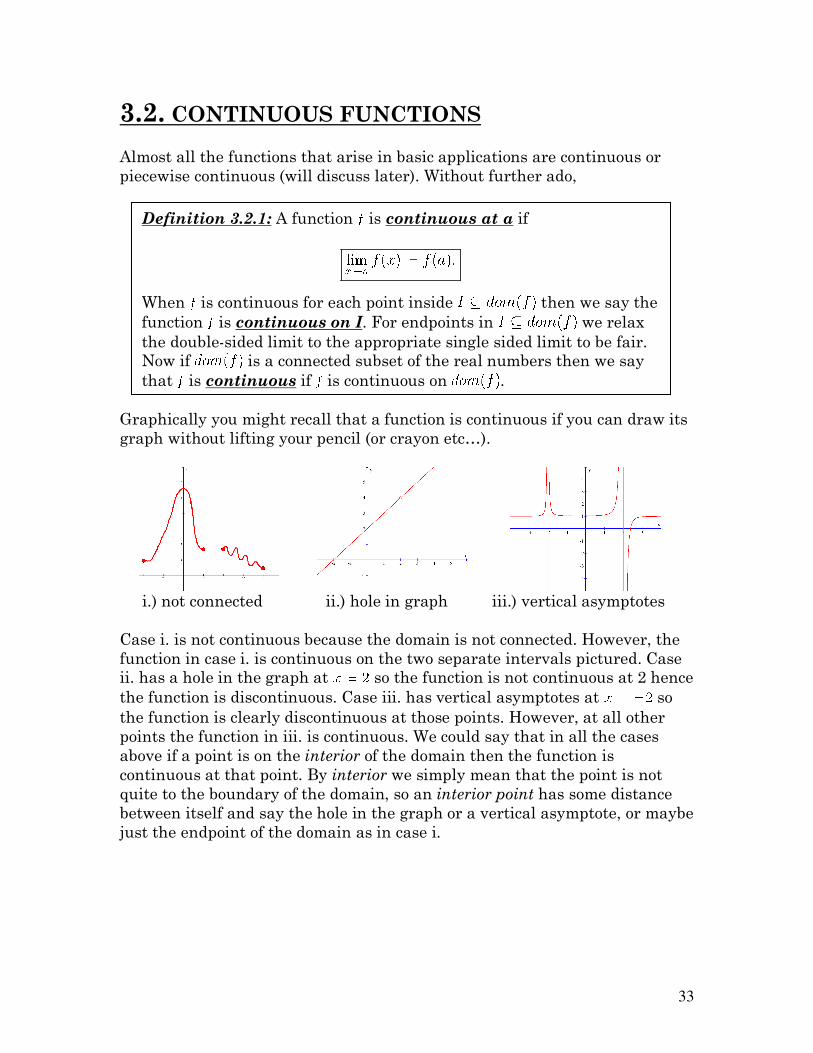
Graphically you might recall that a function is continuous if you can draw its

graph without lifting your pencil (or crayon etc…).

i.) not connected ii.) hole in graph iii.) vertical asymptotes

Case i. is not continuous because the domain is not connected. However, the

function in case i. is continuous on the two separate intervals pictured. Case

ii. has a hole in the graph at so the function is not continuous at 2 hence

the function is discontinuous. Case iii. has vertical asymptotes at so

the function is clearly discontinuous at those points. However, at all other

points the function in iii. is continuous. We could say that in all the cases

above if a point is on the interior of the domain then the function is

continuous at that point. By interior we simply mean that the point is not

quite to the boundary of the domain, so an interior point has some distance

between itself and say the hole in the graph or a vertical asymptote, or maybe

just the endpoint of the domain as in case i.

Definition 3.2.1: A function is continuous at a if

When is continuous for each point inside then we say the

function is continuous on I. For endpoints in we relax

the double-sided limit to the appropriate single sided limit to be fair.

Now if is a connected subset of the real numbers then we say

that is continuous if is continuous on .

34

3.3. EVALUATING BASIC LIMITS

Customarily the theorem which I am about to give is motivated by a longer

discussion of limits. My philosophy is that it is better to just state this

theorem so we can use it. The proof of the theorem actually follows from the

properties of limits which I give in the section after this. Anyway, this

theorem is very important, perhaps the most important theorem I will give

you concerning continuity. It gives the basic building blocks we have to use.

In other words polynomial, rational, algebraic, trigonometric, exponential,

logarithmic, hyperbolic trigonometric, etc… discussed in 2.4 are continuous

where their formulas make sense. If we are not at a vertical asymptote or

hole in the graph then elementary functions are continuous. I should mention

that there exist non-elementary functions which are discontinuous

everywhere. Those sort of functions arise in the study of fractals.

I may ask you to calculate a particular limit a particular way. However, if I

don’t say one way or the other you are free to think for yourself. Sometimes a

graph is a good solution, sometimes a table of values is convenient,

sometimes we can use Theorem 3.3.1 or properties I’ll discuss in the next

section. The example below illustrates the table of values idea.

Theorem 3.3.1: The elementary functions given in section 2.4 are all

continuous at each point in the interior of their domains.

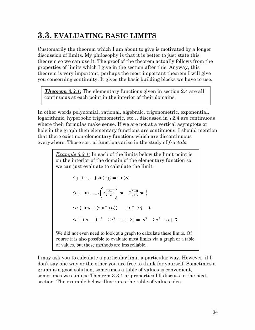
Example 3.3.1: In each of the limits below the limit point is

on the interior of the domain of the elementary function so

we can just evaluate to calculate the limit.

We did not even need to look at a graph to calculate these limits. Of

course it is also possible to evaluate most limits via a graph or a table

of values, but those methods are less reliable..

35

Now the limit consider in Example 3.3.2 is not nearly as obvious as the limits

in Example 3.3.1. I should mention that the limit has indeterminant form of

type 0/0 since both and tend to zero as goes to zero. One of main

goals in this chapter is to learn how to analyze indeterminant forms. I do not

recommend the table of values method for most problems. It will work, but

it’s kind of like painting your car with a paint brush. I do it once, but

probably not when I was trying to impress anybody. It is a good way to gain

intuition about a limit, but I would like to see us use more solid arguments

for the final argument.

Indeterminant forms:

The first three of these we encounter most often. We will need to wait a little

bit before we tackle some of the trickier cases. But, just to give you an idea of

all the different ways a limit can be undetermined, here they are.

• We say that is of “type ” if and .

• We say that is of “type ” if and .

• We say that is of “type ” if and .

• We say that is of “type ” if and .

• We say that is of “type ” if and .

• We say that is of “type ” if and .

• We say that is of “type ” if and .

When we encounter such limits we have to do some thinking and/or work to

unravel the indeterminancy. We saw the table of values revealed the mystery

of in Example 3.3.2. We will learn better methods in future sections.

Example 3.3.2: Using a table of values to see

x sin(x)/x

0.5 0.958851

0.2 0.993347

0.1 0.998334

0.01 0.999983

0.001 0.999999

36

3.4. PROPERTIES OF LIMITS

The notation is meant to include left, right and double-sided limits.

It should be emphasized that we need to know that the limits of both

functions exist for this proposition to work. You cannot just glibly say

and so . This kind of

reasoning is not allowed because there are cases where it fails. It could be

that or 2 or 3 or -75 or 42 etc… it is undetermined. We need to

know that and or else we cannot break up limits as described

in Proposition 3.4.1. Ok, enough about what not to do, let’s see what we can do.

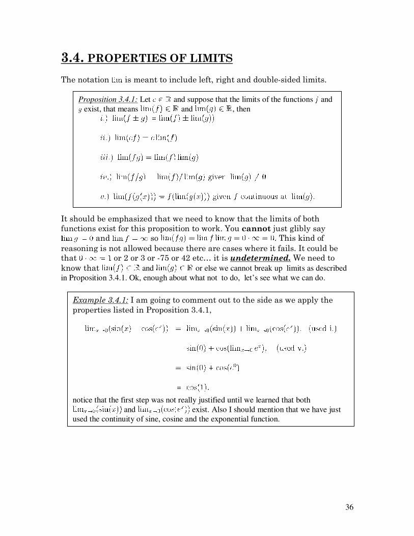
Proposition 3.4.1: Let and suppose that the limits of the functions and

exist, that means and , then

Example 3.4.1: I am going to comment out to the side as we apply the

properties listed in Proposition 3.4.1,

notice that the first step was not really justified until we learned that both

and exist. Also I should mention that we have just

used the continuity of sine, cosine and the exponential function.

37

3.5. ALGEBRAICALLY DETERMINING LIMITS

We have established all the basics. Now it is time for us to do some real

thinking. The examples given in this section illustrate all the basic algebra

tricks to unravel undetermined limits. I like to say we do algebra to

determine the limit. The limits are not just decoration, many times an

expression with the limit is correct while the same expression without the

limit is incorrect. On the other hand we should not write the limit if we do not

need it in the end. How do we know when and when not? We practice.

Example 3.5.1:

Notice that this limit is of type 0/0 since the numerator and denominator are

both zero when take the limit at -2.

The second step where we cancelled with is valid inside

the limit because we do not have in the limit. We get very

close, but that is the difference, this is not division by zero.

Example 3.5.2: The limit below is also type 0/0 to begin with,

I reiterate, we can cancel the inside the limit because within

the limit. Again we see that factoring and cancellation has allowed

us to modify the limit so that we could reasonably plug in the limit

point in the simplified limit. This is often the goal.

38

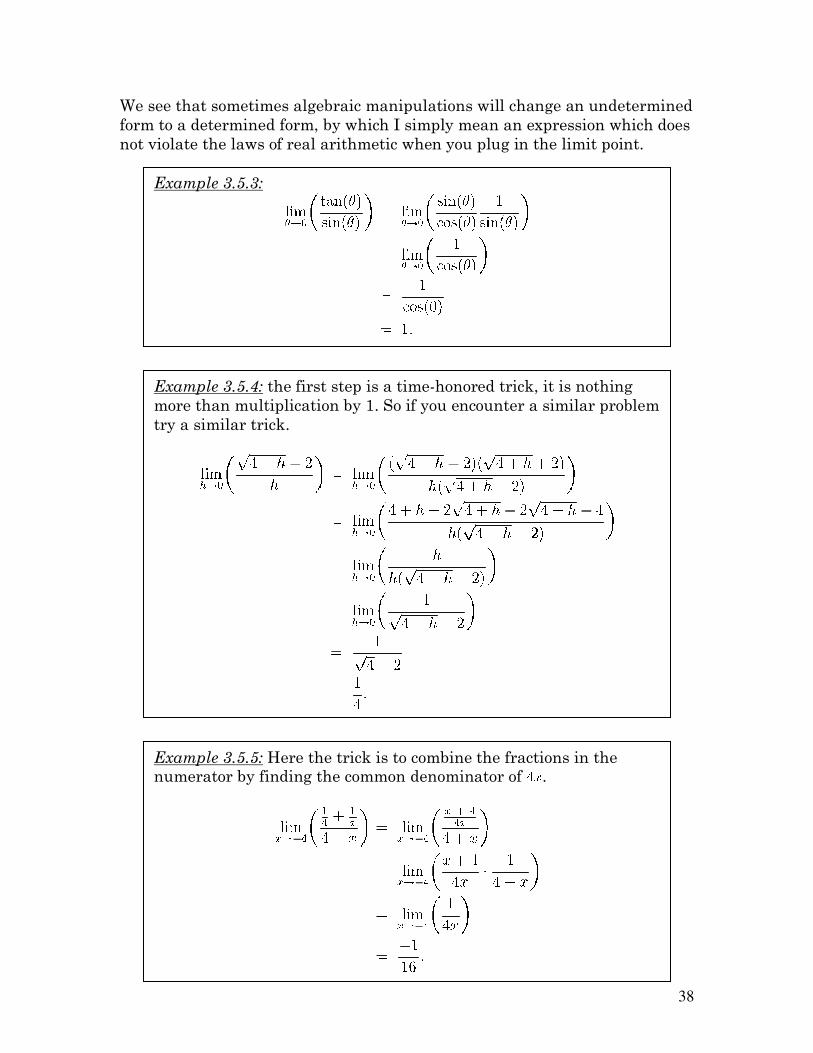
We see that sometimes algebraic manipulations will change an undetermined

form to a determined form, by which I simply mean an expression which does

not violate the laws of real arithmetic when you plug in the limit point.

Example 3.5.3:

Example 3.5.4: the first step is a time-honored trick, it is nothing

more than multiplication by 1. So if you encounter a similar problem

try a similar trick.

Example 3.5.5: Here the trick is to combine the fractions in the

numerator by finding the common denominator of .

39

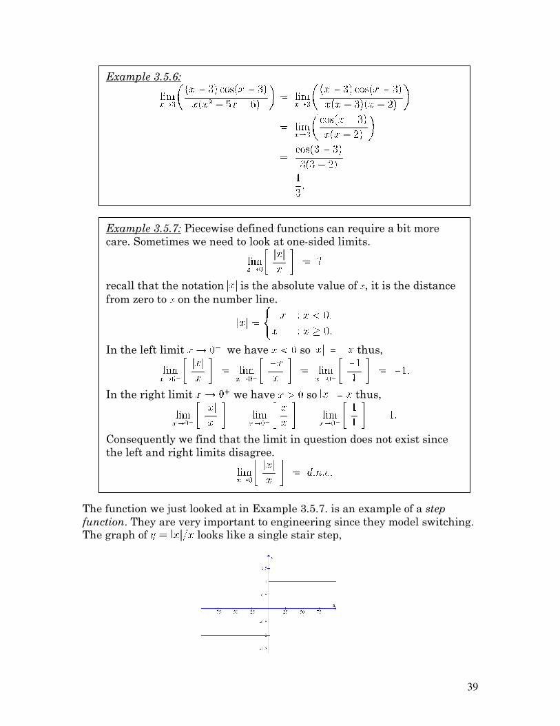
The function we just looked at in Example 3.5.7. is an example of a step

function. They are very important to engineering since they model switching.

The graph of looks like a single stair step,

Example 3.5.7: Piecewise defined functions can require a bit more

care. Sometimes we need to look at one-sided limits.

recall that the notation is the absolute value of , it is the distance

from zero to on the number line.

In the left limit we have so thus,

In the right limit we have so thus,

Consequently we find that the limit in question does not exist since

the left and right limits disagree.

Example 3.5.6:

40

3.6. SQUEEZE THEOREM

There are limits not easily solved through algebraic trickery. Sometimes the

“Squeeze” or “Sandwich” Theorem allows us to calculate the limit.

We can think of as the top slice of the sandwich and as the bottom

slice. The function provides the BBQ or peanut butter or whatever you

want to put in there.

Incidentally, you might be wondering why we could not just use Proposition

3.4.1 part iii. The problem is that since the limit of at zero does not

exist (if you look at the graph of the function you’ll see that it oscillates

wildly near zero) we have no right to apply the proposition.

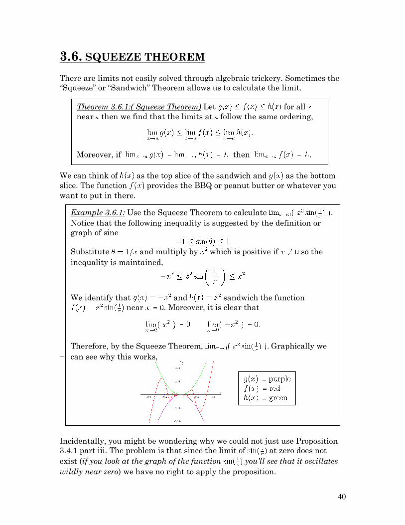
Example 3.6.1: Use the Squeeze Theorem to calculate

Notice that the following inequality is suggested by the definition or

graph of sine

Substitute and multiply by which is positive if so the

inequality is maintained,

We identify that and sandwich the function

near . Moreover, it is clear that

Therefore, by the Squeeze Theorem, Graphically we

can see why this works,

Theorem 3.6.1:( Squeeze Theorem) Let for all

near then we find that the limits at follow the same ordering,

Moreover, if then .

41

3.7. INTERMEDIATE VALUE THEOREM

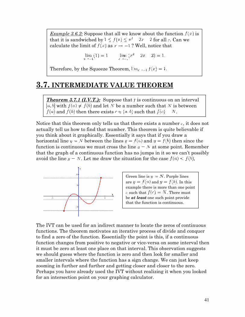
Notice that this theorem only tells us that there exists a number , it does not

actually tell us how to find that number. This theorem is quite believable if

you think about it graphically. Essentially it says that if you draw a

horizontal line between the lines and then since the

function is continuous we must cross the line at some point. Remember

that the graph of a continuous function has no jumps in it so we can’t possibly

avoid the line . Let me draw the situation for the case ,

The IVT can be used for an indirect manner to locate the zeros of continuous

functions. The theorem motivates an iterative process of divide and conquer

to find a zero of the function. Essentially the point is this, if a continuous

function changes from positive to negative or vice-versa on some interval then

it must be zero at least one place on that interval. This observation suggests

we should guess where the function is zero and then look for smaller and

smaller intervals where the function has a sign change. We can just keep

zooming in further and further and getting closer and closer to the zero.

Perhaps you have already used the IVT without realizing it when you looked

for an intersection point on your graphing calculator.

Green line is . Purple lines

are and . In this

example there is more than one point

such that . There must

be at least one such point provide

that the function is continuous.

Example 3.6.2: Suppose that all we know about the function is

that it is sandwiched by for all . Can we

calculate the limit of as ? Well, notice that

Therefore, by the Squeeze Theorem,

Theorem 3.7.1 (I.V.T.): Suppose that is continuous on an interval

with and let be a number such that is between

and then there exists such that .

42

Let me take a moment to write an algorithm to find roots. Suppose we are

given a continuous function , we wish to find such that .

1.) Guess that is zero on some interval .

2.) Calculate and if they have opposite signs go on to 3.)

otherwise return to 1.) and guess differently.

3.) Pick and calculate .

4.) If the sign of matches then say , and let

If the sign of matches then say , and let .

5.) Pick and calculate .

6.) If the sign of matches then say , and let

If the sign of matches then say , and let .

And so on… If we ever found then we stop there. Otherwise, we can

repeat this process until the subinterval is so small we know the zero

to some desired accuracy. Say you wanted to know 2 decimals with certainty,

if you did the iteration until the length of the interval was 0.001 then

you would be more than certain.

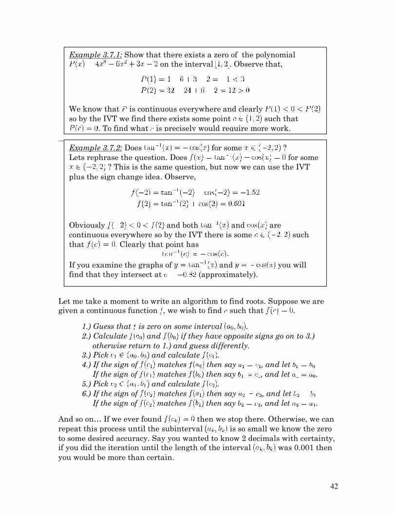
Example 3.7.1: Show that there exists a zero of the polynomial

on the interval . Observe that,

We know that is continuous everywhere and clearly

so by the IVT we find there exists some point such that

. To find what is precisely would require more work.

Example 3.7.2: Does for some ?

Lets rephrase the question. Does for some

? This is the same question, but now we can use the IVT

plus the sign change idea. Observe,

Obviously and both and are

continuous everywhere so by the IVT there is some such

that Clearly that point has

If you examine the graphs of and you will

find that they intersect at (approximately).

43

3.8. PRECISE DEFINITION OF LIMIT

You might read the article by Dr. Monty C. Kester posted on Blackboard. It

helps motivate the definition I give now.

Notice we do not require that the limit point be in the domain of the function.

The zero in is precise way of saying that we do not consider the

limit point in the limit. All other that are within units of the limit point

are included in the analysis ( recall that gives the distance from a to b

on the number line). If the limit exists then we can choose the such that the

values are within units of the limiting value .

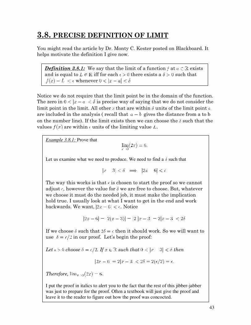
Definition 3.8.1: We say that the limit of a function at exists

and is equal to iff for each there exists a such that

whenever

Example 3.8.1: Prove that

Let us examine what we need to produce. We need to find a such that

The way this works is that is chosen to start the proof so we cannot

adjust , however the value for we are free to choose. But, whatever

we choose it must do the needed job, it must make the implication

hold true. I usually look at what I want to get in the end and work

backwards. We want, . Notice

If we choose such that then it should work. So we will want to

use in our proof. Let’s begin the proof:

Let choose . If such that then

Therefore,

I put the proof in italics to alert you to the fact that the rest of this jibber-jabber

was just to prepare for the proof. Often a textbook will just give the proof and

leave it to the reader to figure out how the proof was concocted.

44

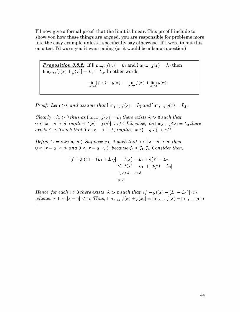
I’ll now give a formal proof that the limit is linear. This proof I include to

show you how these things are argued, you are responsible for problems more

like the easy example unless I specifically say otherwise. If I were to put this

on a test I’d warn you it was coming (or it would be a bonus question)

Proof: Let and assume that and .

Clearly thus as there exists such that

implies . Likewise, as there

exists such that implies .

Define . Suppose such that then

and because . Consider then,

Hence, for each there exists such that

whenever . Thus,

.

Proposition 3.8.2: If and then

. In other words,

45

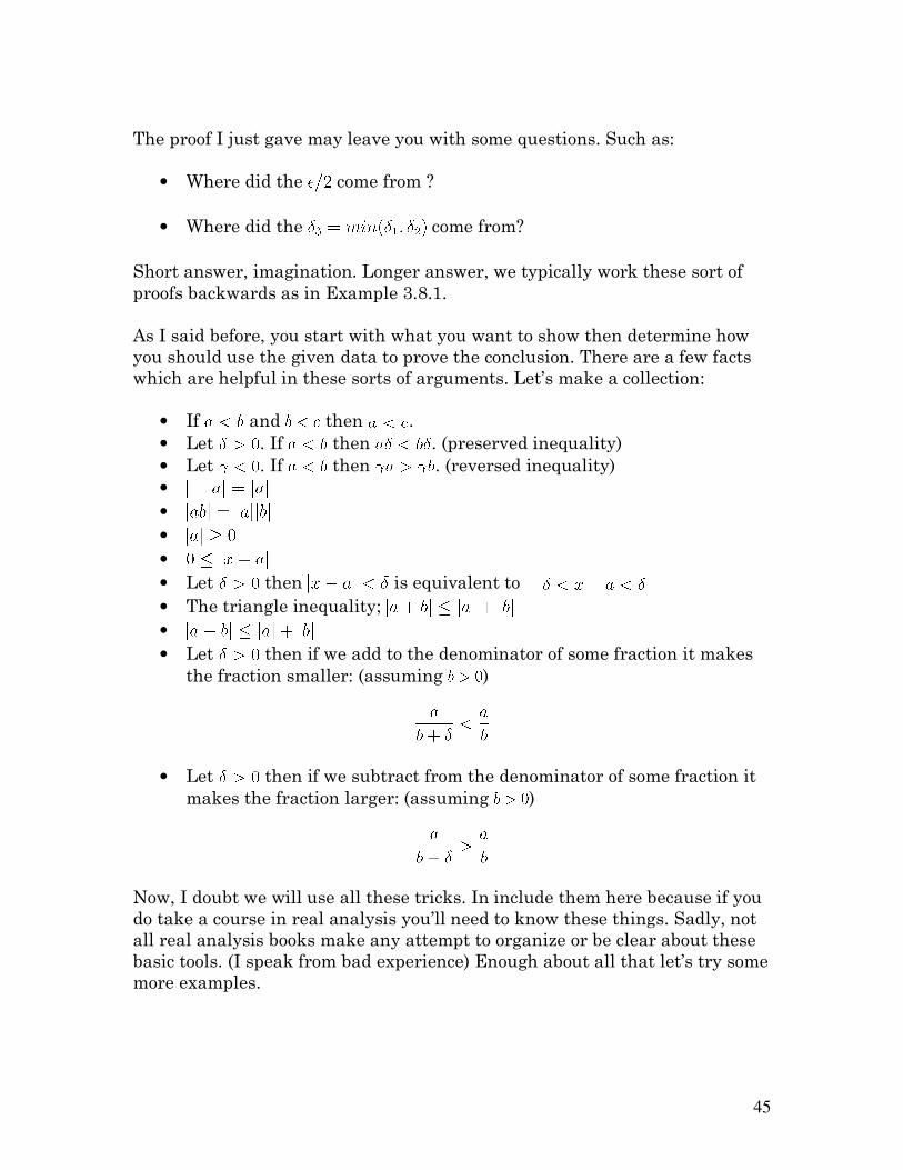
The proof I just gave may leave you with some questions. Such as:

• Where did the come from ?

• Where did the come from?

Short answer, imagination. Longer answer, we typically work these sort of

proofs backwards as in Example 3.8.1.

As I said before, you start with what you want to show then determine how

you should use the given data to prove the conclusion. There are a few facts

which are helpful in these sorts of arguments. Let’s make a collection:

• If and then .

• Let . If then . (preserved inequality)

• Let . If then . (reversed inequality)

•

•

•

•

• Let then is equivalent to

• The triangle inequality;

•

• Let then if we add to the denominator of some fraction it makes

the fraction smaller: (assuming )

• Let then if we subtract from the denominator of some fraction it

makes the fraction larger: (assuming )

Now, I doubt we will use all these tricks. In include them here because if you

do take a course in real analysis you’ll need to know these things. Sadly, not

all real analysis books make any attempt to organize or be clear about these

basic tools. (I speak from bad experience) Enough about all that let’s try some

more examples.

46

The text also discusses a technical definition for what is meant by limits that

go to infinity or negative infinity. We will not cover those this semester. You

will have a problem like Example 3.8.1 or 3.8.2 on the first test. It will be

worth 10 points.

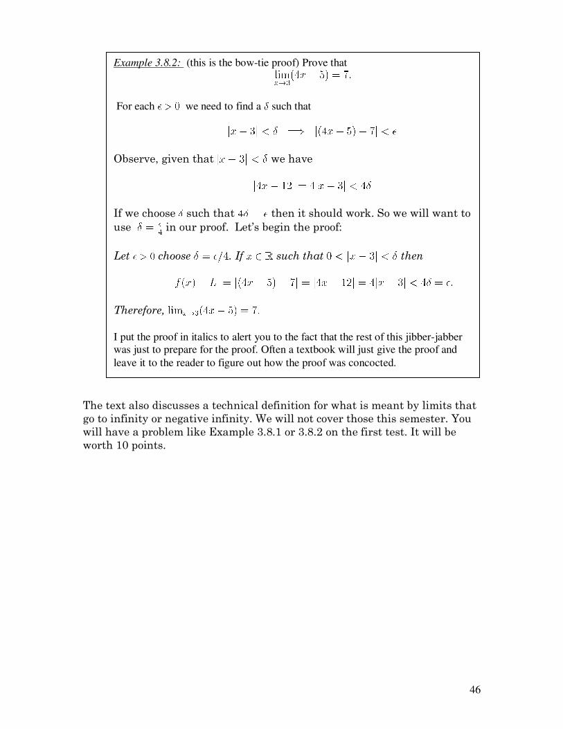
Example 3.8.2: (this is the bow-tie proof) Prove that

For each we need to find a such that

Observe, given that we have

If we choose such that then it should work. So we will want to

use in our proof. Let’s begin the proof:

Let choose . If such that then

Therefore,

I put the proof in italics to alert you to the fact that the rest of this jibber-jabber

was just to prepare for the proof. Often a textbook will just give the proof and

leave it to the reader to figure out how the proof was concocted.

47

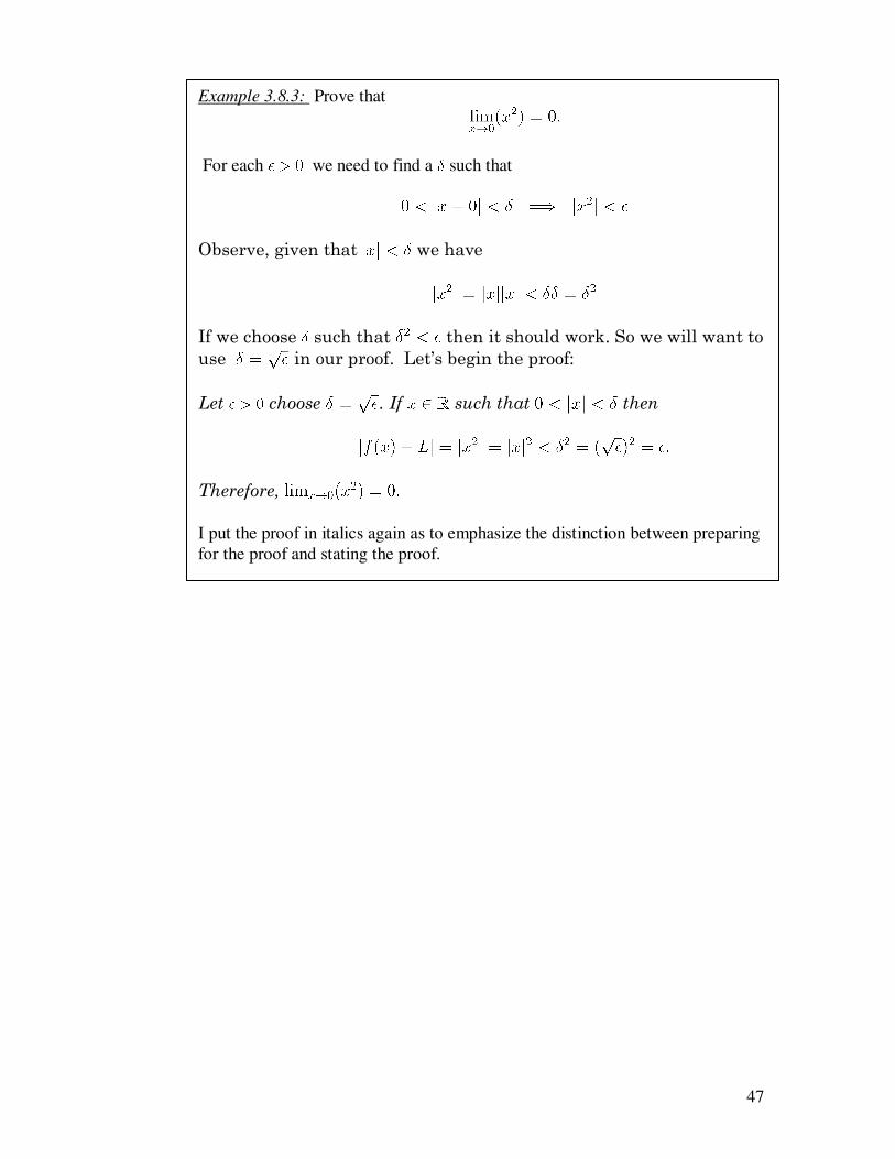
Example 3.8.3: Prove that

For each we need to find a such that

Observe, given that we have

If we choose such that then it should work. So we will want to

use in our proof. Let’s begin the proof:

Let choose . If such that then

Therefore,

I put the proof in italics again as to emphasize the distinction between preparing

for the proof and stating the proof.