Chapter 3 Kinematics

In the first place, what do we mean by time and space? It turns out that these deep philosophical questions have to be analyzed very carefully in physics, and this is not easy to do. The theory of relativity shows that our ideas of space and time are not as simple as one might imagine at first sight. However, for our present purposes, for the accuracy that we need at first, we need not be very careful about defining things precisely. Perhaps you say, “That’s a terrible thing—I learned that in science we have to define everything precisely.” We cannot define anything precisely! If we attempt to, we get into that paralysis of thought that comes to philosophers, who sit opposite each other, one saying to the other, “You don’t know what you are talking about!” The second one says. “What do you mean by know? What do you mean by talking? What do you mean by you?”, and so on. In order to be able to talk constructively, we just have to agree that we are talking roughly about the same thing. You know as much about time as you need for the present, but remember that there are some subtleties that have to be discussed; we shall discuss them later. Richard Feynman , The Feynman Lectures on Physics1

Part A: One-Dimensional Motion Introduction Kinematics is the mathematical description of motion. The term is derived from the Greek word kinema, meaning movement. In order to quantify motion, a mathematical coordinate system, called a reference frame, is used to describe space and time. Once a reference frame has been chosen, we can introduce the physical concepts of position, velocity and acceleration in a mathematically precise manner. Figure 3.1 shows a Cartesian coordinate system in one dimension with unit vector pointing in the direction of increasing

ix -coordinate.

Figure 3.1 A one-dimensional Cartesian coordinate system.

1 Richard P. Feynman, Robert B. Leighton, Matthew Sands, The Feynman Lectures on Physics, Addison-Wesley, Reading, Massachusetts, (1963), p. 12-2.

9/5/2008 1

3.1 Position, Time Interval, Displacement Position Consider an object moving in one dimension. We denote the position coordinate of the center of mass of the object with respect to the choice of origin by ( )x t . The position coordinate is a function of time and can be positive, zero, or negative, depending on the location of the object. The position has both direction and magnitude, and hence is a vector (Figure 3.2), ˆ( ) ( )t x t=x i . (3.1.1)

We denote the position coordinate of the center of the mass at 0t = by the symbol

. The SI unit for position is the meter [m] (see Section 1.3). 0 ( 0x x t≡ = )

Figure 3.2 The position vector, with reference to a chosen origin. Time Interval Consider a closed interval of time . We characterize this time interval by the difference in endpoints of the interval such that

1 2[ , ]t t

2t t t1Δ = − . (3.1.2)

The SI units for time intervals are seconds [s]. Definition: Displacement

The change in position coordinate of the mass between the times and is 1t 2t 2 1

ˆ( ( ) ( )) ( ) ˆx t x t x tΔ ≡ − ≡ Δx i i . (3.1.3)

This is called the displacement between the times and (Figure 3.3). Displacement is a vector quantity.

1t 2t

9/5/2008 2

Figure 3.3 The displacement vector of an object over a time interval is the vector difference between the two position vectors

3.2 Velocity When describing the motion of objects, words like “speed” and “velocity” are used in common language; however when introducing a mathematical description of motion, we need to define these terms precisely. Our procedure will be to define average quantities for finite intervals of time and then examine what happens in the limit as the time interval becomes infinitesimally small. This will lead us to the mathematical concept that velocity at an instant in time is the derivative of the position with respect to time. Definition: Average Velocity

The component of the average velocity, xv , for a time interval is defined to be the displacement

tΔxΔ divided by the time interval tΔ ,

xxvt

Δ≡Δ

. (3.2.1)

The average velocity vector is then

ˆ( ) ( )xxt vt

ˆtΔ≡ =Δ

v i i . (3.2.2)

The SI units for average velocity are meters per second 1m s−⎡ ⎤⋅⎣ ⎦ . Instantaneous Velocity Consider a body moving in one direction. We denote the position coordinate of the body by ( )x t , with initial position 0x at time 0t = . Consider the time interval [ , . The average velocity for the interval

]t t t+ ΔtΔ is the slope of the line connecting the points ( ,

and . The slope, the rise over the run, is the change in position over the change in time, and is given by

( ))t x t( , ( ))t x t t+ Δ

9/5/2008 3

rise ( ) ( )runx

x x t t x tvt t

Δ + Δ −≡ = =

Δ Δ. (3.2.3)

Let’s see what happens to the average velocity as we shrink the size of the time interval. The slope of the line connecting the points ( and , ( ))t x t ( , ( ))t x t t+ Δ approaches the slope of the tangent line to the curve ( )x t at the time (Figure 3.4). t

Figure 3.4 Graph of position vs. time showing the tangent line at time . t In order to define the limiting value for the slope at any time, we choose a time interval . For each value of [ , ]t t t+ Δ tΔ , we calculate the average velocity. As , we generate a sequence of average velocities. The limiting value of this sequence is defined to be the

0tΔ →

x -component of the instantaneous velocity at the time . t Definition: Instantaneous Velocity

The x -component of instantaneous velocity at time t is given by the slope of the tangent line to the curve of position vs. time curve at time : t

0 0 0

( ) ( )( ) lim lim limx xt t t

x x t t x t dxv t vt tΔ → Δ → Δ → dt

Δ + Δ −≡ = = ≡

Δ Δ. (3.2.4)

The instantaneous velocity vector is then ˆ( ) ( )xt v t=v i . (3.2.5) Example 1: Determining Velocity from Position Consider an object that is moving along the x -coordinate axis represented by the equation

9/5/2008 4

20

1( )2

x t x bt= + (3.2.6)

where 0x is the initial position of the object at 0t = . We can explicitly calculate the x -component of instantaneous velocity from Equation (3.2.4) by first calculating the displacement in the x -direction, ( ) ( )x x t t x tΔ = + Δ − . We need to calculate the position at time t t+ Δ ,

(2 20 0

1 1( ) ( ) 22 2 )2x t t x b t t x b t t t t+ Δ = + + Δ = + + Δ + Δ . (3.2.7)

Then the instantaneous velocity is

2 20 0

0 0

1 1( 2 )( ) ( ) 2 2( ) lim limx t t

2x b t t t t x btx t t x tv t

t tΔ → Δ →

⎛ ⎞ ⎛+ + Δ + Δ − +⎜ ⎟ ⎜+ Δ − ⎝ ⎠ ⎝= =Δ Δ

⎞⎟⎠ . (3.2.8)

This expression reduces to

0

1( ) lim2x t

v t bt b tΔ →

⎛ ⎞= + Δ⎜⎝ ⎠

⎟ . (3.2.9)

The first term is independent of the interval tΔ and the second term vanishes because the limit as of is zero. Thus the instantaneous velocity at time t is 0tΔ → tΔ ( )xv t bt= . (3.2.10) In Figure 3.5 we graph the instantaneous velocity, , as a function of time . ( )xv t t

Figure 3.5 A graph of instantaneous velocity as a function of time.

9/5/2008 5

3.3 Acceleration We shall apply the same physical and mathematical procedure for defining acceleration, the rate of change of velocity. We first consider how the instantaneous velocity changes over an interval of time and then take the limit as the time interval approaches zero. Average Acceleration Acceleration is the quantity that measures a change in velocity over a particular time interval. Suppose during a time interval tΔ a body undergoes a change in velocity ( ) (t t t)Δ = + Δ −v v v . (3.3.1) The change in the x -component of the velocity, xvΔ , for the time interval [ is then

, ]t t t+ Δ

( ) (x x xv v t t v t)Δ = + Δ − . (3.3.2) Definition: Average Acceleration

The x -component of the average acceleration for the time interval is defined to be

tΔ

( ( ) ( ))ˆ ˆ ˆ ˆx x xx

v v t t v t vat t t

Δ + Δ −= ≡ = = xΔ

Δ Δa i i i

Δi . (3.3.3)

The SI units for average acceleration are meters per second squared, . 2[m s ]−⋅ Instantaneous Acceleration On a graph of the x -component of velocity vs. time, the average acceleration for a time interval is the slope of the straight line connecting the two points ( and

. In order to define the tΔ , ( ))xt v t

( , (xt t v t t+ Δ + Δ )) x -component of the instantaneous acceleration at time t , we employ the same limiting argument as we did when we defined the instantaneous velocity in terms of the slope of the tangent line. Definition: Instantaneous Acceleration.

The x -component of the instantaneous acceleration at time is the limit of the slope of the tangent line at time t of the graph of the

tx -component of the velocity

as a function of time,

9/5/2008 6

0 0 0

( ( ) ( ))( ) lim lim limx x xx xt t t

v t t v t v dva t at tΔ → Δ → Δ →

x

dt+ Δ − Δ

≡ = = ≡Δ Δ

. (3.3.4)

The instantaneous acceleration vector is then ˆ( ) ( )xt a t=a i . (3.3.5) In Figure 3.6 we illustrate this geometrical construction.

Figure 3.6 Graph of velocity vs. time showing the tangent line at time . t Since velocity is the derivative of position with respect to time, the x -component of the acceleration is the second derivative of the position function,

2

2x

xdv d xadt dt

= = . (3.3.6)

Example 2: Determining Acceleration from Velocity Let’s continue Example 1, in which the position function for the body is given by

20 (1/ 2)x x= + bt , and the x -component of the velocity is xv bt= . The x -component of

the instantaneous acceleration at time is the limit of the slope of the tangent line at time of the graph of the

tt x -component of the velocity as a function of time (Figure 3.5)

0 0

( ) ( )lim limx x xx t t

dv v t t v t bt b t bta bdt t tΔ → Δ →

+ Δ − + Δ −= = = =

Δ Δ. (3.3.7)

Note that in Equation (3.3.7), the ratio /v tΔ Δ is independent of tΔ , consistent with the constant slope of the graph in Figure 3.4.

9/5/2008 7

3.4 Constant Acceleration Let’s consider a body undergoing constant acceleration for a time interval . When the acceleration

[0, ]t tΔ =

xa is a constant, the average acceleration is equal to the instantaneous acceleration. Denote the x -component of the velocity at time by

. Therefore the 0t =

,0 ( 0x xv v t≡ = ) x -component of the acceleration is given by

,0( )x xxx x

v t vva at t

−Δ= = =

Δ. (3.4.1)

Thus the velocity as a function of time is given by ,0( )x x xv t v a t= + . (3.4.2) When the acceleration is constant, the velocity is a linear function of time. Velocity: Area Under the Acceleration vs. Time Graph In Figure 3.7, the x -component of the acceleration is graphed as a function of time.

Figure 3.7 Graph of the x -component of the acceleration for xa constant as a function of time.

The area under the acceleration vs. time graph, for the time interval 0t t tΔ = − = , is

Area( , )x xa t a t≡ . (3.4.3) Using the definition of average acceleration given above, ,0Area( , ) ( )x x x xa t a t v v t vx≡ = Δ = − . (3.4.4)

9/5/2008 8

Displacement: Area Under the Velocity vs. Time Graph In Figure 3.8, we graph the x -component of the velocity vs. time curve.

Figure 3.8 Graph of velocity as a function of time for xa constant. The region under the velocity vs. time curve is a trapezoid, formed from a rectangle and a triangle and the area of the trapezoid is given by

(,0 ,01Area( , ) ( )2x x x xv t v t v t v t= + − ) . (3.4.5)

Substituting for the velocity (Equation (3.4.2)) yields

2,0 ,0 ,0 ,0

1Area( , ) ( )2 2x x x x x x xv t v t v a t v t v t a t= + + − = +

1 . (3.4.6)

Figure 3.9 The average velocity over a time interval. We can then determine the average velocity by adding the initial and final velocities and dividing by a factor of two (see Figure 3.9).

,01 ( ( ) )2x x xv v t v= + . (3.4.7)

9/5/2008 9

The above method for determining the average velocity differs from the definition of average velocity in Equation (3.2.1). When the acceleration is constant over a time interval, the two methods will give identical results. Substitute into Equation (3.4.7) the x -component of the velocity, Equation (3.4.2), to yield

( ) ( )( ),0 ,0 ,0 ,01 1( )2 2

12x x x x x x xv v t v v a t v v a= + = + + = + x t . (3.4.8)

Recall Equation (3.2.1); the average velocity is the displacement divided by the time interval (note we are now using the definition of average velocity that always holds, for non-constant as well as constant acceleration). The displacement is equal to 0( ) xx x t x v tΔ ≡ − = . (3.4.9) Substituting Equation (3.4.8) into Equation (3.4.9) shows that displacement is given by

20 ,0

1( )2x x xx x t x v t v t a tΔ ≡ − = = + . (3.4.10)

Now compare Equation (3.4.10) to Equation (3.4.6) to conclude that the displacement is equal to the area under the graph of the x -component of the velocity vs. time,

20 ,0

1( ) Area( , ),2x x xx x t x v t a t v tΔ ≡ − = + = (3.4.11)

and so we can solve Equation (3.4.11) for the position as a function of time,

20 ,0

1( )2x xx t x v t a t= + + . (3.4.12)

Figure 3.10 shows a graph of this equation. Notice that at 0t = the slope may be in general non-zero, corresponding to the initial velocity component ,0xv .

9/5/2008 10

Figure 3.10 Graph of position vs. time for constant acceleration. 3.5 Integration and Kinematics Change of Velocity as the Integral of Non-constant Acceleration When the acceleration is a non-constant function, we would like to know how the x -component of the velocity changes for a time interval [0, ]t tΔ = . Since the acceleration is non-constant we cannot simply multiply the acceleration by the time interval. We shall calculate the change in the x -component of the velocity for a small time interval

and sum over these results. We then take the limit as the time intervals become very small and the summation becomes an integral of the

1[ , ]i i it t t +Δ ≡x -component of the

acceleration. For a time interval , we divide the interval up into small intervals

, where the index , and [0, ]tΔ = t N

1[ , ]i i it t t +Δ ≡ 1, 2, ... ,i N= 1 0t ≡ , Nt t≡ . Over the interval , we

can approximate the acceleration as a constant, itΔ

( )x ia t . Then the change in the x -component of the velocity is the area under the acceleration vs. time curve, , 1( ) ( ) ( )x i x i x i x i iv v t v t a t t E+Δ ≡ − = Δ + i (3.5.1) where is the error term (see Figure 3.11a). Then the sum of the changes in the iE x -component of the velocity is

(3.5.2) , 2 1 3 21

( ( ) ( 0)) ( ( ) ( )) ( ( ) ( )).i N

x i x x x x x N x Ni

v v t v t v t v t v t t v t=

−=

Δ = − = + − + + = −∑ 1

In this summation pairs of terms of the form ( )2 2( ) ( ) 0x xv t v t− = sum to zero, and the overall sum becomes

,1

( ) (0)i N

x xi

v t v v=

=x i− = Δ∑ . (3.5.3)

Substituting Equation (3.5.1) into Equation (3.5.3),

,1 1

( ) (0) ( )i N i N i N

1x x x i x i i

i i iv t v v a t t E

= = =

= = =

− = Δ = Δ + i∑ ∑ ∑ . (3.5.4)

We now approximate the area under the graph in Figure 3.11a by summing up all the rectangular area terms,

9/5/2008 11

1

Area ( , ) ( )i N

N x x i ii

a t a t t=

=

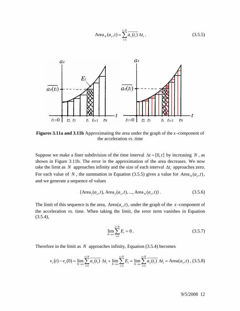
= Δ∑ . (3.5.5)

Figures 3.11a and 3.11b Approximating the area under the graph of the x -component of the acceleration vs. time

Suppose we make a finer subdivision of the time interval [0, ]t tΔ = by increasing , as shown in Figure 3.11b. The error in the approximation of the area decreases. We now take the limit as approaches infinity and the size of each interval

N

N itΔ approaches zero. For each value of , the summation in Equation N (3.5.5) gives a value for , and we generate a sequence of values

Area ( , )N xa t

. (3.5.6) 1 2{Area ( , ), Area ( , ), ..., Area ( , )}x x Na t a t a tx

The limit of this sequence is the area, , under the graph of the Area( , )xa t x -component of the acceleration vs. time. When taking the limit, the error term vanishes in Equation (3.5.4),

1

lim 0i N

iN iE

=

→∞=

=∑ . (3.5.7)

Therefore in the limit as approaches infinity, Equation N (3.5.4) becomes

1 1 1

( ) (0) lim ( ) lim lim ( ) Area( , )i N i N i N

x x x i i i x i i xN N Ni i iv t v a t t E a t t a t

= = =

→∞ →∞ →∞= = =

− = Δ + = Δ =∑ ∑ ∑ , (3.5.8)

9/5/2008 12

and thus the change in the x -component of the velocity is equal to the area under the graph of x -component of the acceleration vs. time. Definition: Integral of acceleration

The integral of the x -component of the acceleration for the interval [0 is defined to be the limit of the sequence of areas, , and is denoted by

, ]tArea ( , )N xa t

. (3.5.9) 0 10

( ) lim ( ) Area( , )i

t t i N

x x i it it

a t dt a t t a t′= =

Δ →=′=

′ ′ ≡ Δ =∑∫ x

Equation (3.5.8) shows that the change in the x –component of the velocity is the integral of the x -component of the acceleration with respect to time.

0

( ) (0) ( )t t

x x xt

v t v a t dt′=

′=

′ ′− = ∫ . (3.5.10)

Using integration techniques, we can in principle find the expressions for the velocity as a function of time for any acceleration. Integral of Velocity We can repeat the same argument for approximating the area A under the graph of the

rea( , )xv tx -component of the velocity vs. time by subdividing the time interval into

intervals and approximating the area by N

1

Area ( , ) ( )i N

N x x i ii

a t v t t=

=

= Δ∑ . (3.5.11)

The displacement for a time interval [0, ]t tΔ = is limit of the sequence of sums

, Area ( , )N xa t

1

( ) (0) lim ( )i N

x iN iix x t x v t t

=

→∞=

Δ = − = Δ∑ . (3.5.12)

This approximation is shown in Figure 3.12.

9/5/2008 13

Figure 3.12 Approximating the area under the graph of the x -component of the velocity vs. time. Definition: Integral of Velocity

The integral of the x -component of the velocity for the interval [ is the limit of the sequence of areas, , and is denoted by

0, ]tArea ( , )N xa t

. (3.5.13) 0 10

( ) lim ( ) Area( , )i

t t i N

x x i it it

v t dt v t t v t′= =

Δ →=′=

′ ′ ≡ Δ =∑∫ x

The displacement is then the integral of the x -component of the velocity with respect to time,

0

( ) (0) ( )t t

xt

x x t x v t dt′=

′=

′ ′Δ = − = ∫ . (3.5.14)

Using integration techniques, we can in principle find the expressions for the position as a function of time for any acceleration. Example: Let’s consider a case in which the acceleration, , is not constant in time, ( )xa t (3.5.15) 2

0 1 2( )xa t b b t b t= + + The graph of the x -component of the acceleration vs. time is shown in Figure 3.13

9/5/2008 14

Figure 3.13 A non-constant acceleration vs. time graph. Let’s find the change in the x -component of the velocity as a function of time. Denote the initial velocity at by 0t = ,0 ( 0x xv v t )≡ = . Then,

2 3

2 1 2,0 1 2 0

0 0

( ) ( ) ( )2 3

t t t t

x x x ot t

b t b tv t v a t dt b b t b t dt b t′ ′= =

′ ′= =

′ ′ ′ ′ ′− = = + + = + +∫ ∫ . (3.5.16)

The x -component of the velocity as a function in time is then

2 3

1 2,0 0( )

2 3x xb t b tv t v b t= + + + . (3.5.17)

Denote the initial position by 0 ( 0x x t )≡ = . The displacement as a function of time is the integral

00

( ) ( ) .t t

xt

x t x v t dt′=

′=

′ ′− = ∫ (3.5.18)

Use Equation (3.5.17) for the x -component of the velocity in Equation (3.5.18) to find

2 3 2 3

1 2 0 1 20 ,0 0 ,0

0

( ) .2 3 2 6 12

t t

x xt

b t b t b t b t b tx t x v b t dt v t′=

′=

′ ′⎛ ⎞′ ′− = + + + = + + +⎜ ⎟

⎝ ⎠∫

4

(3.5.19)

Finally the position is then

9/5/2008 15

2 3

0 1 20 ,0( ) .

2 6 12xb t b t b tx t x v t= + + + +

4

(3.5.20)

3.6 Free Fall An important example of one-dimensional motion (for both scientific and historical reasons) is an object undergoing free fall. Suppose you are holding a stone and throw it straight up in the air. For simplicity, we’ll neglect all the effects of air resistance. The stone will rise and fall along a line, and so the stone is moving in one dimension. Galileo Galilei was the first to definitively state that all objects fall towards the earth with a constant acceleration, later measured to be of magnitude 29.8 m sg −= ⋅ to two significant figures (see Section 4.3). The symbol will always denote the magnitude of the acceleration at the surface of the earth. (We will later see that Newton’s Universal Law of Gravitation requires some modification of Galileo’s statement, but near the earth’s surface his statement holds.) Let’s choose a coordinate system with the origin located at the ground, and the -axis perpendicular to the ground with the -coordinate increasing in the upward direction. With our choice of coordinate system, the acceleration is constant and negative,

g

y y

2( ) 9.8 m s .ya t g −= − = − ⋅ (3.6.1)

When we ignore the effects of air resistance, the acceleration of any object in free fall near the surface of the earth is downward, constant and equal to 29.8 m s−⋅ .

Of course, if more precise numerical results are desired, a more precise value of must be used (see Section 4.3).

g

Equations of Motions We have already determined the position equation (Equation (3.4.12)) and velocity equation (Equation (3.4.2)) for an object undergoing constant acceleration. With a simple change of variables from x y→ , the two equations of motion for a freely falling object are

20 ,0

1( )2yy t y v t g t= + − (3.6.2)

and ,0( )y yv t v g t= − , (3.6.3)

9/5/2008 16

where 0y is the initial position from which the stone was released at , and is the initial

0t = ,0yvy -component of velocity that the stone acquired at 0t = from the act of throwing.

Part B: Two-Dimensional Motion 3.7 Introduction to the Vector Description of Motion in Two and Three Dimensions So far we have introduced the concepts of kinematics to describe motion in one dimension; however we live in a multidimensional universe. In order to explore and describe motion in this universe, we begin by looking at examples of two-dimensional motion, of which there are many; planets orbiting a star in elliptical orbits or a projectile moving under the action of uniform gravitation are two common examples. We will now extend our definitions of position, velocity, and acceleration for an object that moves in two dimensions (in a plane) by treating each direction independently, which we can do with vector quantities by resolving each of these quantities into components. For example, our definition of velocity as the derivative of position holds for each component separately. In Cartesian coordinates, in which the directions of the unit vectors do not change from place to place, the position vector

with respect to some choice of origin for the object at time is given by ( )tr t ˆ( ) ( ) ( )t x t y t= +r i j . (3.7.1) The velocity vector at time t is the derivative of the position vector, ( )tv

( ) ( )ˆ ˆ ˆ( ) ( ) ( )x ydx t dy tt v t

dt dt= + ≡ +v i ˆv tj i j , (3.7.2)

where and ( ) ( ) /xv t dx t dt≡ ( ) ( ) /yv t dy t dt≡ denote the x - and -components of the velocity respectively.

y

The acceleration vector is defined in a similar fashion as the derivative of the velocity vector,

( )ta

( )( ) ˆ ˆ ˆ( ) ( ) ( ) ,yx

x y

dv tdv tt a tdt dt

= + ≡ +a i ˆa tj i j (3.7.3)

where and ( ) ( ) /x xa t dv t dt≡ ( ) ( ) /y ya t dv t dt≡ denote the x - and y -components of the acceleration.

9/5/2008 17

3.8 Projectile Motion A special case of two-dimensional motion occurs when the vertical component of the acceleration is constant and the horizontal component is zero. Then the complete set of equations for position and velocity for each independent direction of motion are given by

( ) 20 ,0 0 ,0

1ˆ ˆ ˆ( ) ( ) ( )2x yt x t y t x v t y v t a t⎛= + = + + + +⎜

⎝ ⎠r i ˆ

y⎞⎟j i j , (3.8.1)

( ),0 ,0

ˆ ˆ ˆ( ) ( ) ( )x y x y yt v t v t v v a t= + = + +v i ˆj i j , (3.8.2) ˆ ˆ( ) ( ) ( ) ˆ

x yt a t a t a= + =a i yj j . (3.8.3) Consider the motion of a body that is released with an initial velocity at a height h above the ground. Two paths are shown in Figure 3.14.

0v

Figure 3.14 Actual orbit and parabolic orbit of a projectile The dotted path represents a parabolic trajectory and the solid path represents the actual orbit. The difference between the paths is due to air resistance. There are other factors that can influence the path of motion; a rotating body or a special shape can alter the flow of air around the body, which may induce a curved motion or lift like the flight of a baseball or golf ball. We shall begin our analysis by neglecting all influences on the body except for the influence of gravity. We shall choose coordinates with our y -axis in the vertical direction with j directed upwards and our x-axis in the horizontal direction with i directed in the direction that the body is moving horizontally. We choose our origin to be the place where the body is released at time 0t = . Figure 3.15 shows our coordinate system with the position of the body at time t and the coordinate functions ( )x t and ( )y t .

9/5/2008 18

Figure 3.15 A coordinate sketch for parabolic motion. The coordinate function represents the distance from the body to the origin along the -axis at time t , and the coordinate function

( )y ty ( )x t represents the distance from the

body to the origin along the x -axis at time t . The y -component of the acceleration, ,ya g= − (3.8.4) is a constant and is independent of the mass of the body. Notice that ; this is because we chose our positive -direction to point upwards.

0ya <y

Since we are ignoring the effects of any horizontal forces, the acceleration in the horizontal direction is zero, 0;xa = (3.8.5) therefore the x -component of the velocity remains unchanged throughout the flight. Kinematic Equations of Motion The kinematic equations of motion for the position and velocity components of the object are 0 ,0( ) xx t x v t= + , (3.8.6) ,0( )x xv t v= , (3.8.7)

20 ,0

1( )2yy t y v t g t= + − , (3.8.8)

9/5/2008 19

,0( )y yv t v g t= − . (3.8.9) Initial Conditions In these equations, the initial velocity vector is 0 ,0 ,

ˆ( ) x yt v v= +v i 0 j . (3.8.10) Often the description of the flight of a projectile includes the statement, “a body is projected with an initial speed at an angle 0v 0θ with respect to the horizontal.” The vector decomposition diagram for the initial velocity is shown in Figure 3.16. The components of the initial velocity are given by ,0 0 0cosxv v θ= , (3.8.11) ,0 0 0sinyv v θ= . (3.8.12)

Figure 3.16 A vector decomposition of the initial velocity Since the initial speed is the magnitude of the initial velocity, we have

( )1/ 22 20 ,0 ,0x yv v v= + . (3.8.13)

The angle 0θ is related to the components of the initial velocity by

,010

,0

tan .y

x

vv

θ −⎛ ⎞

= ⎜ ⎟⎜ ⎟⎝ ⎠

(3.8.14)

The initial position vector appears with components 0 0 0

ˆ ˆx y= +r i j . (3.8.15)

9/5/2008 20

Note that the trajectory in Figure 3.16 has 0 0 0x y= = , but this will not always be the case, as in the analysis below Orbit equation So far our description of the motion has emphasized the independence of the spatial dimensions, treating all of the kinematic quantities as functions of time. We shall now eliminate time from our equation and find the orbit equation of the body. We begin with Equation (3.8.6) for the x -component of the position, 0 ,0( ) xx t x v t= + (3.8.16) and solve Equation (3.8.16) for time t as a function of ( )x t ,

0

,0

( )

x

x t xtv−

= . (3.8.17)

The vertical position of the body is given by Equation (3.8.8),

20 ,0

1( ) .2yy t y v t g t= + − (3.8.18)

We then substitute the above expression, Equation (3.8.17) for time t into our equation for the y -component of the position yielding

2

00 ,0

,0 ,0

( ) 1 ( )( )2y

x x

0x t x x t xy t y v gv v

⎛ ⎞ ⎛ ⎞−= + −⎜ ⎟ ⎜⎜ ⎟ ⎜

⎝ ⎠ ⎝ ⎠

−⎟⎟ . (3.8.19)

This expression can be simplified to give

( ) (,0 20 0 2

,0 ,0

1( ) ( ) ( ) 2 ( )2

y

x x

v g )20 0y t y x t x x t x t x x

v v= + − − − + . (3.8.20)

This is seen to be an equation for a parabola by rearranging terms to find

,0 ,02 200 02 2 2

,0 ,0 ,0 ,0 ,0

1 1( ) ( ) ( ) .2 2

y y

x x x x x

v vg g x g0y t x t x t x x

v v v v v⎛ ⎞

= − + + − − +⎜ ⎟⎜ ⎟⎝ ⎠

y (3.8.21)

The graph of ( )y t as a function of ( )x t is shown in Figure 3.17.

9/5/2008 21

Figure 3.17 The parabolic orbit Note that at any point ( ( ), ( ))x t y t along the parabolic trajectory, the direction of the tangent line at that point makes an angle θ with the positive x -axis as shown in Figure 3.17. This angle is given by

1tan dydx

θ − ⎛= ⎜⎝ ⎠

⎞⎟ , (3.8.22)

where is the derivative of the function /dy dx ( ) ( ( ))y x y x t= at the point ( )( ), ( )x t y t . The velocity vector is given by

( ) ( )ˆ ˆ ˆ( ) ( ) ( )x ydx t dy tt v t

dt dt= + ≡ +v i ˆv tj i j (3.8.23)

The direction of the velocity vector at a point ( )( ), ( )x t y t can be determined from the components. Let φ be the angle that the velocity vector forms with respect to the positive x -axis. Then

1 1 1( ) /tan tan tan .( ) /

y

x

v t dy dt dyv t dx dt dx

φ − − −⎛ ⎞ ⎛ ⎞ ⎛= = =⎜ ⎟ ⎜ ⎟ ⎜⎝ ⎠ ⎝⎝ ⎠

⎞⎟⎠

(3.8.24)

Comparing our two expressions we see that φ θ= ; the slope of the graph of ( )y t vs. ( )x t at any point determines the direction of the velocity at that point. We cannot tell from our graph of ( )y x how fast the body moves along the curve; the magnitude of the velocity cannot be determined from information about the tangent line.

9/5/2008 22

If, as in Figure 4.16, we choose our origin at the initial position of the body at , then and . Our orbit equation, Equation 0t = 0 0x = 0 0y = (3.8.21) can now be

simplified to

,022,0 ,0

1( ) ( ) ( ).2

y

x x

vgy t x tv v

= − + x t (3.8.25)

Part C: Non-Constant Acceleration 3.9 Friction as a linear function of velocity. We have seen an example where the acceleration of an object was a given non-constant function of time, Equation (3.5.15). In many physical situations the force on an object will be modeled as depending on the object’s velocity. (Forces will be discussed in Chapter 4 and will be indispensable in the rest of this subject.) Some friction models result in an acceleration that is proportional to the velocity, γ= −a v , (3.9.1) where γ is a constant that depends on the properties (density, viscosity) of the medium and the size and shape of the object. Note that γ has dimensions of inverse time,

[ ][ ]

21

1

dim acceleration L Tdim[ ] Tdim velocity L T

γ−

−−

⋅= =

⋅= . (3.9.2)

The minus sign in Equation Error! Reference source not found. indicates that the acceleration is directed opposite to that of the object’s velocity (relative to the fluid). The acceleration has no component perpendicular to the velocity, and in the absence of other forces an object with this acceleration will move in a straight line, but with varying speed. Denote the direction of this motion as the x -direction, so that Equation (3.9.1) becomes

xx x

d vadt

vγ= = − . (3.9.3)

Equation (3.9.3) is now a differential equation. For our purposes, we’ll create an initial-condition problem by specifying that the initial x -component of velocity is 0( 0) xv t v= = . Two methods of solving this problem, both used by physicists, will be presented here.

9/5/2008 23

The first is the use of an ansatz2 ; from Equation (3.9.3) we would expect a graph of xv as a function of time to start at 0xv with a negative slope, and since xv is decreasing we expect the slope to decrease. There are many such functions. What we do for an ansatz is to pick a specific functional form that has the desired shape and see how, if at all, the function can be made to satisfy Equation (3.9.3) and the initial condition 0( 0) xv t v= = . Two such functions are considered here:

1/1 0

2 02

1 ,1 /

tv v e

v vt

τ

τ

−=

=+

(3.9.4)

where 1τ and 2τ are constants with dimensions of time that may have to be determined. The two functions and are plotted in Figure 3.18 below. For Plotting purposes, the vertical scale is the ratio or and the horizontal scale is

1v 2v

1 0/v v 2 0/v v /t τ=t . The upper plot (the green plot if viewed in color) is and the lower (red) is . It should be clear that both plots have the desired qualitative property of decreasing with decreasing slope.

2v 1v

We still need to see which of either of the expressions in (3.9.4) satisfy both Equation (3.9.3) and the initial condition 0( 0) xv t v= = . Both satisfy the initial condition, and indeed the leading factor could be changed as desired to match any initial condition. Performing the differentiations,

( )

1/10 1

1 1

220 22

2 02

1 1

1 1 1 .1 /

td v v e vdt

d v v vdt vt

τ

τ τ

τ ττ

−= − = −

= − = −+ 2

(3.9.5)

Thus, as given in the second expression in 2v (3.9.4) cannot be a solution to (3.9.3). We see that will be a solution if we choose 1v 1/τ γ= , with the result 0

txv v e γ−= . (3.9.6)

2 A mathematical assumption, esp. about the form of an unknown function, which is made in order to facilitate solution of an equation or other problem. Oxford English Dictionary. In other words, an inspired guess.

9/5/2008 24

Figure 3.18 Plots of the trial functions

Note that even though the chosen form for did not work for this problem, we see that if we encountered a similar problem with the magnitude of the acceleration proportional to the square of the speed, we’ve got that one solved, if we remember where we did it. (Such a dependence of friction on speed is known as Newtonian Damping, so we suspect it’s worth knowing.)

2v

The differential equation in (3.9.3) is known as a separable equation, in that the equation may be rewritten as

[ ]1 lnxx

x

d v d vv dt dt

γ= = − . (3.9.7)

The integration in this case is simple, leading to

[ ] [ ]0

0

ln ln

,

x

tx

v tv ev

γ

γ

−

= − +

=

v (3.9.8)

reproducing the result of Equation (3.9.6) It should be noted that the result in Equation (3.9.7) is sometimes obtained by “cross-multiplying” the expression in (3.9.3) to obtain

9/5/2008 25

x

x

d v dtv

γ= − (3.9.9)

and then integrating both sides with respect to the respective integration variables, to obtain the same result. This is indeed equivalent to making a “change of variables” in the calculus wording. 3.10 Linear Friction with Gravity A common extension of the above example is to have an object falling through the same viscous medium, subject to gravity but no other forces. Taking the positive y -direction to be downward, the equation of motion becomes

yy

d va g

dt yvγ= = − . (3.10.1)

Note that the expression in Equation (3.10.1) is valid for the vertical velocity directed upwards ( ) or downwards ( ). Unlike the previous example, there is a preferred direction; we expect that in the limit of long times and no other forces, any object would eventually fall straight down. We will use the expectation to simplify our methods of solution, starting with an ansatz that assumes a terminal velocity (actually, a terminal speed) ; the terminal velocity is that for which the acceleration given by Equation

0yv < 0yv >

termv(3.10.1) is zero, term /v g γ= (note that has dimensions of velocity). At this

point, it helps to rewrite Equation termv

(3.10.1) as

( termy

y

d vv v

dtγ= − )

yv yv

. (3.10.2)

If we have, as before, an initial-value problem, in this case the initial condition being

, our trial solution will be one that has 0(0)yv = 0(0)yv = but which approaches for large times. From our previous experience, we suspect that a function involving an exponential will be more likely to lead to success than a rational function. So, our trial function will be

termv

( ) 3/

3 term 0 termtv v v v e τ−= + − . (3.10.3)

Performing the differentiation,

( )

( )

3/30 term

3

3 term3

1

1

td v v v edt

v v

τ

τ

τ

−= − −

= − − (3.10.4)

9/5/2008 26

and we see that is a solution to the problem with the choice 3v 3 1/τ γ= ; ( )term 0 term

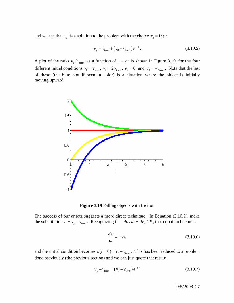
tyv v v v e γ−= + − . (3.10.5)

A plot of the ratio as a function of term/yv v tγ=t is shown in Figure 3.19, for the four different initial conditions , 0 termv v= 0 te2v v rm 0 0v = and 0 tev v= , rm= − . Note that the last of these (the blue plot if seen in color) is a situation where the object is initially moving upward.

Figure 3.19 Falling objects with friction

The success of our ansatz suggests a more direct technique. In Equation (3.10.2), make the substitution . Recognizing that termyu v v= − / /ydu dt dv dt= , that equation becomes

d u udt

γ= − (3.10.6)

and the initial condition becomes 0 ter( 0)u t v v m= = − . This has been reduced to a problem done previously (the previous section) and we can just quote that result; ( )term 0 term

tyv v v v e γ−− = − (3.10.7)

9/5/2008 27

and we’re done. If we hadn’t seen to do this, Equation (3.10.2) is still separable,

termterm

1 lnyy

y

d v d v vv v dt dt

γ⎡ ⎤= − −⎣ ⎦−= − . (3.10.8)

Integrating and exponentiating, including the initial condition,

[ ]

( )term term 0

term term 0

ln ln

,y

ty

v v t v v

v v v v e γ

γ−

⎡ ⎤− = − + −⎣ ⎦− = −

(3.10.9)

reproducing the previous result. In the result, the behavior of the solution should be checked in the large and small limits of time. From the graphs, or from the analytic form, as . For small times

termyv v→ t →∞1/t γ , consider the solution expressed as

( )( )

( )

term 0

0

0

0

1

1

t ty

t t

v v e v e

g e v e

g t v

g t v

γ γ

γ γ

γ

γγ

− −

− −

= − +

= − +

+

= +

(3.10.10)

to zero order in γ , as expected.

9/5/2008 28