Chapter 3 · Chapter 3 Introduction to QM/MM Simulations Gerrit Groenhof Abstract Hybrid quantum mechanics/molecular mechanics (QM/MM) simulations have become a popular tool for

Chapter 3

Introduction to QM/MM Simulations

Gerrit Groenhof

Abstract

Hybrid quantum mechanics/molecular mechanics (QM/MM) simulations have become a popular tool forinvestigating chemical reactions in condensed phases. In QM/MM methods, the region of the system inwhich the chemical process takes place is treated at an appropriate level of quantum chemistry theory, whilethe remainder is described by a molecular mechanics force field. Within this approach, chemical reactivitycan be studied in large systems, such as enzymes. In the first part of this contribution, the basic methodol-ogy is briefly reviewed. The two most common approaches for partitioning the two subsystems arepresented, followed by a discussion on the different ways of treating interactions between the subsystems.Special attention is given on how to deal with situations in which the boundary between the QM and MMsubsystems runs through one or more chemical bonds. The second part of this contribution discusses whatproperties of larger system can be obtained within the QM/MM framework and how. Finally, as an exampleof a QM/MM application in practice, the third part presents an overview of recent QM/MM moleculardynamics simulations on photobiological systems. In addition to providing quantities that are experimen-tally accessible, such as structural intermediates, fluorescence lifetimes, quantum yields and spectra, theQM/MM simulations also provide information that is much more difficult to measure experimentally, suchas reaction mechanisms and the influence of individual amino acid residues.

Key word: Quantum mechanics, Molecular mechanics, QM/MM, Molecular dynamics

1. Introduction

In this chapter we present a short introduction into the developmentand application of computational techniques for modelling chemi-cal reactions in the condensed phase.We start by reviewing the basicconcepts of these methods. We then discuss how these methods canbe used in practical computations and what kind of information canbe obtained. We conclude this chapter with a short review of anapplication on a photobiological system, for which the simulationsnot only revealed the detailed sequence of events that follow photonabsorption but also demonstrate how the biological environmentcontrols the photochemical reaction.

Luca Monticelli and Emppu Salonen (eds.), Biomolecular Simulations: Methods and Protocols, Methods in Molecular Biology,vol. 924, DOI 10.1007/978-1-62703-017-5_3, # Springer Science+Business Media New York 2013

43

2. QM/MM: Theoryand Implementation

The size and complexity of a typical biomolecular system, togetherwith the timescales that must be reached, necessitate the use ofclassical molecular dynamics for the nuclear degrees of freedom.In molecular dynamics (MD) simulations, Newton’s equations ofmotion are solved numerically to obtain a trajectory of the dynamicsof a molecule over a period of time (1). To model electronic rear-rangements during a chemical reaction, a quantum mechanicaldescription (QM) is required for those parts of the system that areinvolved in the reaction. For the remainder, a simple molecularmechanics force field model suffices (MM). The interactions in thesystem are thus computed within a hybrid QM/MM framework.

2.1. Molecular

Mechanics

Molecular dynamics simulations of biological systems have come ofage (2). Since the first application of MD on a small protein invacuum more than three decades ago (3), advances in computerpower, algorithmic developments and improvements in the accu-racy of the used interaction functions have established MD as animportant and predictive technique to study dynamic processes atatomic resolution (4). In the interaction functions, the so-calledmolecular mechanics force field, simple chemical concepts are usedto describe the potential energy of the system (1):

VMM ¼XN bonds

iV bond

i þXN angles

jV j þ

XN torsions

lV torsion

l

þXNMM

i

XNMM

j>iV Coul

ij þXNMM

i

XNMM

j>iV LJ

ij ; (1)

whereNMM is the number of atoms in the system. Bonds and angles(Vbond, Vangle) are normally modelled by harmonic functions, andtorsions by periodic functions (V torsion). The pairwise electrostaticinteraction between atoms with a partial charge (Qi) is given byCoulomb’s law:

V Coulij ¼ e2Q iQ j

4pE0Rij ;(2)

in whichRij denotes the interatomic distance, e the unit charge andE0 the dielectric constant. Van der Waals interactions, for examplethe combination of short-range Pauli repulsion and long-rangedispersion attraction, are most often modelled by the Lennard-Jones potential:

V LJij ¼ Cij

12

Rij

!12

� Cij6

Rij

!6

; (3)

44 G. Groenhof

with C12ij and C6

ij a repulsion and attraction parameter, respec-tively, which depend on the atomtypes of the atoms i and j.

Electrons are thus ignored in molecular mechanics force fields.Their influence is expressed by empirical parameters that are validfor the ground state of a given covalent structure. Therefore,processes that involve electronic rearrangements, such as chemicalreactions, cannot be described at the MM level. Instead, theseprocesses require a quantum mechanics description of the elec-tronic degrees of freedom. However, the computational demandfor evaluating the electronic structure places severe constraints onthe size of the system that can be studied.

2.2. Hybrid Quantum

Mechanics/Molecular

Mechanics Models

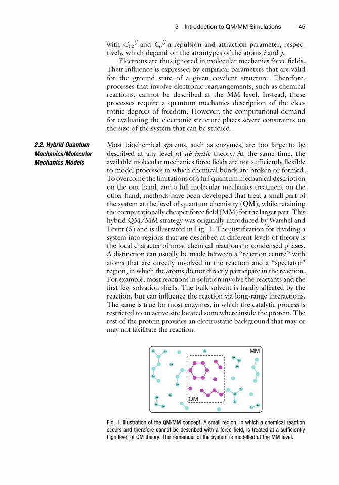
Most biochemical systems, such as enzymes, are too large to bedescribed at any level of ab initio theory. At the same time, theavailable molecular mechanics force fields are not sufficiently flexibleto model processes in which chemical bonds are broken or formed.To overcome the limitations of a full quantummechanical descriptionon the one hand, and a full molecular mechanics treatment on theother hand, methods have been developed that treat a small part ofthe system at the level of quantum chemistry (QM), while retainingthe computationally cheaper force field (MM) for the larger part. Thishybrid QM/MM strategy was originally introduced by Warshel andLevitt (5) and is illustrated in Fig. 1. The justification for dividing asystem into regions that are described at different levels of theory isthe local character of most chemical reactions in condensed phases.A distinction can usually be made between a “reaction centre” withatoms that are directly involved in the reaction and a “spectator”region, in which the atoms do not directly participate in the reaction.For example, most reactions in solution involve the reactants and thefirst few solvation shells. The bulk solvent is hardly affected by thereaction, but can influence the reaction via long-range interactions.The same is true for most enzymes, in which the catalytic process isrestricted to an active site located somewhere inside the protein. Therest of the protein provides an electrostatic background that may ormay not facilitate the reaction.

Fig. 1. Illustration of the QM/MM concept. A small region, in which a chemical reactionoccurs and therefore cannot be described with a force field, is treated at a sufficientlyhigh level of QM theory. The remainder of the system is modelled at the MM level.

3 Introduction to QM/MM Simulations 45

The hybrid QM/MM potential energy contains three classes ofinteractions: interactions between atoms in the QM region, betweenatoms in the MM region and interactions between QM and MMatoms. The interactionswithin theQMandMMregions are relativelystraightforward to describe, that is at the QM andMM level, respec-tively. The interactions between the two subsystems aremore difficultto describe, and several approaches have been proposed. Theseapproaches can be roughly divided into two categories: subtractiveand additive coupling schemes.

2.3. Subtractive

QM/MM Coupling

In the subtractive scheme, the QM/MM energy of the system isobtained in three steps. First, the energy of the total system, con-sisting of both QM and MM regions, is evaluated at the MM level.The QM energy of the isolated QM subsystem is added in thesecond step. Third, the MM energy of the QM subsystem is com-puted and subtracted. The last step corrects for including theinteractions within the QM subsystem twice:

VQM=MM ¼ VMMðMMþQMÞ þ VQMðQMÞ � VMMðQMÞ: (4)

The terms QM and MM stand for the atoms in the QM and MMsubsystems, respectively. The subscripts indicate the level of theory atwhich the potential energies (V ) are computed. The most widelyused subtractive QM/MM scheme is the ONIOM method, devel-oped by the Morokuma group (6, 7), and is illustrated in Fig. 2.

The main advantage of the subtractive QM/MM couplingscheme is that no communication is required between the quantumchemistry andmolecular mechanics routines. This makes the imple-mentation relatively straightforward. However, compared to themore advanced schemes that are discussed below, there are alsodisadvantages.

A major disadvantage is that a force field is required for the QMsubsystem, which may not always be available. In addition, the forcefield needs to be sufficiently flexible to describe the effect of chemi-cal changes when a reaction occurs.

δ+

δ–

δ–

δ–

δ–

δ–

δ–

δ–

δ–

δ–

δ–

δ–

δ–

δ–

δ–

δ–

δ–

δ–

δ+

δ+

δ+

δ+

δ+

δ+

δ+

δ+

δ+ δ+

δ+

δ+

δ+

δ+δ+

δ– δ+

δ+

δ+

δ+

δ+

δ+

δ+

δ+

MM

QM

=

QM

+

MM

–

MM

Fig. 2. Subtractive QM/MM coupling: The QM/MM energy of the total system (left hand side of the equation) is assumed tobe equal to the energy of the isolated QM subsystem, evaluated at the QM level, plus the energy of the complete systemevaluated at the MM level, minus the energy of the isolated QM subsystem, evaluated at the MM level. The last term issubtracted to correct for double counting of the contribution of the QM subsystem to the total energy. A prerequisite for thecalculation is that a force field for the QM subsystem is available.

46 G. Groenhof

A further drawback of this method is absence of polarization ofthe QM electron density by the MM environment. This shortcom-ing can be particularly problematic for modelling biological chargetransfer processes, since these are usually mediated by the proteinenvironment. For a realistic description of such reactions a moreconsistent treatment of the interactions between the electrons andtheir surrounding environment is needed.

2.4. Additive QM/MM

Coupling

In additive schemes, the QM system is embedded within the largerMM system, and the potential energy for the whole system is a sumof MM energy terms, QM energy terms and QM/MM couplingterms:

VQM=MM ¼ VQMðQMÞ þ VMMðMMÞ þ V QM�MMðQMþMMÞ:(5)

Here, only the interactionswithin theMMregion are described at theforce field level, VMM(MM). In contrast to the subtractive scheme,the interactions between the two subsystems are treated explicitly:VQM�MMðQM+MMÞ. These interactions can be described at variousdegrees of sophistication.

2.4.1. Mechanical

Embedding

In the most basic approach, all interactions between the two sub-systems are handled at the force field level. The QM subsystem isthus kept in place by MM interactions. This is illustrated in Fig. 3.Chemical bonds between QM and MM atoms are modelled byharmonic potentials (Vbond), angles defined by one QM atom,and two MM atoms are described by the harmonic potential aswell (V angles), while torsions involving at most two QM atoms arecommonly modelled by a periodic potential function (V torsion).Non-bonded interactions, that is those between atoms separatedby three or more atoms, are also modelled by force field terms: Vander Waals by the Lennard-Jones potential (VLJ) and electrostaticsby the Coulomb potential (V Coul). In the most simple implemen-tation of mechanical embedding, the electronic wave function isevaluated for an isolated QM subsystem. Therefore, the MM envi-ronment cannot induce polarization of the electron density in theQM region. For calculating the electrostatic interactions betweenthe subsystems, one can either use a fixed set of charges for the QMregion, for example, those given by the force field, or re-computethe partial charges on the QM atoms at every integration step of thesimulation. In the second strategy, a least-squares fitting procedureis used to derive atomic charges that optimally reproduce theelectrostatic potential at the surface of the QM subsystem (8, 9).

Lennard-Jones parameters are normally not updated. There-fore, problems may arise if during the simulation, changes occur inthe chemical character of the atoms in the QM region, for example,in reactions that involve changes in the hybridization state of the


atoms. However, since the Lennard-Jones potential is a relativelyshort-ranged function, the error introduced by keeping the sameparameters throughout the simulations is most likely not very large.

2.4.2. Electrostatic

Embedding

An improvement of mechanical embedding is to include polarizationeffects. In the electrostatic embedding scheme, the electrostaticinteractions between the two subsystems are handled during the

a b

dc

e f

Fig. 3. Coupling between the QM and MM subsystems in the additive QM/MM schemes. The top panels (a)–(c) showbonded interactions between QM and MM atoms. These interactions are handled at the force field level (MM). Panel dshows the Van der Waals interactions between an atom in the QM region and three MM atoms. These interactions aremodelled by the Lennard-Jones potential. Panel e illustrates the link atom concept. This atom caps the QM subsystem andis present only in the QM calculation. Panel f demonstrates how the electrostatic QM/MM interactions are handled. In theelectrostatic embedding approach, the charged MM atoms enter the electronic Hamiltonian of the QM subsystem. In themechanical embedding, partial MM charges are assigned to the QM atoms and the electrostatic interactions are computedby the pairwise Coulomb potential.

48 G. Groenhof

computation of the electronic wave function. The charged MMatoms enter the QMHamiltonian as one-electron operators:

hQM�MMi ¼ hQM

i �XMJ

e2Q J

4pE0jri �RJ j ; (6)

where ri andRJ are the positions of electron i andMMatom J, hiQM is

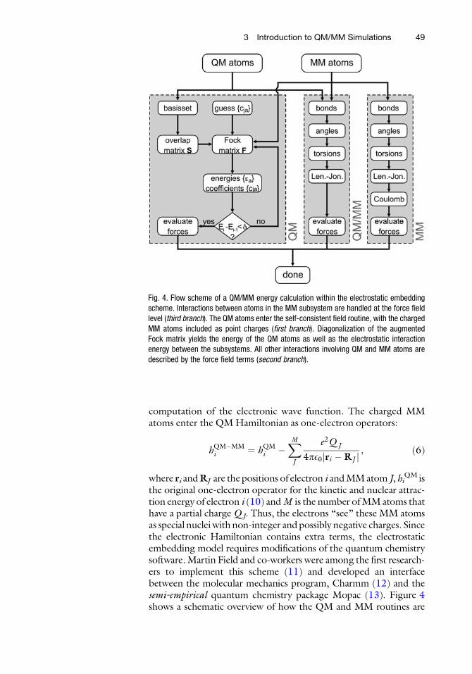
the original one-electron operator for the kinetic and nuclear attrac-tion energy of electron i (10) andM is the number ofMMatoms thathave a partial charge QJ. Thus, the electrons “see” these MM atomsas special nuclei with non-integer and possibly negative charges. Sincethe electronic Hamiltonian contains extra terms, the electrostaticembedding model requires modifications of the quantum chemistrysoftware.Martin Field and co-workers were among the first research-ers to implement this scheme (11) and developed an interfacebetween the molecular mechanics program, Charmm (12) and thesemi-empirical quantum chemistry package Mopac (13). Figure 4shows a schematic overview of how the QM and MM routines are

Fig. 4. Flow scheme of a QM/MM energy calculation within the electrostatic embeddingscheme. Interactions between atoms in the MM subsystem are handled at the force fieldlevel (third branch). The QM atoms enter the self-consistent field routine, with the chargedMM atoms included as point charges (first branch). Diagonalization of the augmentedFock matrix yields the energy of the QM atoms as well as the electrostatic interactionenergy between the subsystems. All other interactions involving QM and MM atoms aredescribed by the force field terms (second branch).


interconnected in a practical implementation of electrostaticembedding. In the electrostatic coupling approach, the MM atomscan polarize the electrons in QM subsystem. However, the atomiccharges of the MM atoms have been parametrized to provide arealistic description of an MM system, rather than of a physicallycorrect charge distribution. Therefore, the question arises whetherpolarization induced by these MM charges is realistic or not.In principle, one would need to re-derive the charges for use inQM/MM frameworks. In reality, interactions between the systemsare not only due to electrostatics between charged atoms, but alsodue to polarization, exchange, charge transfer, dispersion and Paulirepulsion. In force fields, only the combination of atomic charges andLennard-Jones parameters provides a reasonable description ofall these effects taken together, albeit in an implicit manner. Partof the interaction due to polarization of theQMregion is thus alreadyaccounted for by the Lennard-Jones potential. Therefore, not onlytheMM charges, but also the Lennard-Jones parameters would needto be reparametrized for use in electrostatic embedding QM/MMsimulations. However, in practice this is hardly done, andmost work-ers use default force field parameters.

A further problem that may arise when using standard MMatomic charges to describe the charge distribution in the MM sys-tem, is the risk of over-polarization near the boundary. The pointcharges on the MM side of the interface may attract (or repel) theelectrons too strongly, which could lead to electron density spillingout into the MM region. Such artefacts can become serious if largeflexible basis set (e.g., with polarization and diffuse functions), orplane waves are used in the QM calculations. The electron spill outcan be avoided by using smeared-out charges instead of the tradi-tional point charges (14). A convenientway for smearing the chargesis to use a Gaussian distribution centred at the MM atom:

OMMJ ðrÞ ¼

ffiffiffiffiffiffiffiffiffiffiffiffiQMM

J

pa3

sexp � jðr�RJ Þj2

2a2

" #; (7)

where |OJMM(r)|2 is the charge density at position r, due to MM

atom J at position RJ and charge Q J. The factor a controls thewidth of the distribution and is a parameter that needs to becalibrated. In contrast to the point charge model, the Coulombinteraction between the QM electrons and the Gaussian chargedistributions does not diverge if the electrons approach the MMatoms:

hij ðr1Þ ¼ Q J

Zf�i ðr1Þ

erf ðjr1 �RJj=aÞjr1 �RJ j fj ðr1Þdr1; (8)

with fi the molecular orbital and hij the one-electron integraldescribing the interaction of a single electron with MM atom J.Such renormalization of the coulomb interaction avoids the

50 G. Groenhof

unphysical attraction of the electrons to charged atoms at theboundary between the two subsystems.

2.4.3. Polarization

Embedding

The next step in increasing the level of sophistication is to includethe polarizability of the MM atoms. In the polarization embeddingscheme both regions can mutually polarize each other. Thus, notonly is the QM region polarized by the MM atoms, the QM regioncan also induce polarization in the MM system. Differentapproaches have been developed to model polarization of MMatoms. Among the most popular methods are the charge-on-a-spring model (15), the induced dipole model (16) and the fluctu-ating charge model (17).

To obtain the total QM/MM energy in the polarizable embed-ding approach, theMM polarizations need to be computed at everystep of the self consistent-field iteration of the QM wave function.Since the polarization is computed in a self-consistent manner aswell, the QM/MM computation can become very cumbersomeand demanding. As a compromise, Zhang and co-workers havesuggested to include polarization only in a small shell of MMatoms around the QM region (18).

Although polarization embedding offers the most realisticcoupling between the QM and MM regions, polarizable forcefield for biomolecular simulations are not yet available. Therefore,despite progress in the development of such force fields, QM/MMstudies with polarizable MM regions have so far been largelyrestricted to non-biological systems (19).

2.5. Capping Bonds

at the QM/MM Boundary

If the QM and MM subsystems are connected by chemical bonds,care has to be taken when evaluating the QM wave function.A straightforward cut through the QM/MM bond creates one ormore unpaired electrons in the QM subsystem. In reality, theseelectrons are paired in bonding orbitals with electrons belongingto the atom on the MM side. A number of approaches to remedythe artefact of such open valences have been proposed.

2.5.1. Link Atoms The most easy solution is to introduce a monovalent link atom at anappropriate position along the bond vector between the QM andMM atoms (Figs. 3e and 5). Hydrogen is most often used, butthere is no restriction on the type of the link atom and evencomplete fragments, such as methyl groups, can be used tocap the QM subsystem. The link atoms are present only in theQM calculation, and are invisible for the MM atoms. In principleeach link atom introduces three additional degrees of freedom tothe system. However, in practice the link atom is placed at a fixedposition along the bond in every step of the simulation, so thatthese additional degrees of freedom are removed again. At eachstep, the force acting on the link atoms are distributed over the QMand MM atoms of the bond according to the lever rule.


2.5.2. Localized Orbitals A popular alternative to the link atom scheme is to replace achemical bond between the QM and MM subsystem by a double-occupied molecular orbital. This idea, which dates back to thepioneering work of Warshel and Levitt (5), assumes that theelectronic structure of the bond is insensitive to changes in theQM region. The two most widely used approaches are the localizedhybrid orbital method (20), which introduces orbitals at the QMatom (Fig. 5b), and the generalized hybrid orbital approach (21),which places additional orbitals on the MM atom (Fig. 5c).

In the localized self-consistent field (LSCF) method by Rivailand co-workers (20), the atomic orbitals on the QM atom of thebroken bond are localized and hybridized. The hybrid orbitalpointing towards the MM atom is occupied by two electrons. Theother orbitals are each occupied by a single electron. During theSCF optimization of the QM wave function, the double-occupiedorbital is kept frozen, while the other hybrid orbitals are optimizedalong with all orbitals in the QM region. The parameters in thismethod are the molecular orbital coefficients of the hybrid orbitals.In the original approach, these parameters are obtained by localis-ing orbitals in smaller model systems. This procedure thus assumesthat the electronic structure of a chemical bond is transferablebetween different systems.

Alternatively, the coefficients of the frozen orbital can beobtained by performing a single point QM/MM calculation witha slightly enlarged QM subsystem. Any further broken bondsbetween the larger QM subsystem and the MM region are cappedby link atoms in this calculation. The advantage of this so-calledfrozen orbital approach (22) is that no assumption is made on theelectronic structure of the chemical bond. The disadvantage is thatan electronic structure calculation has to be performed on a largerQM subsystem.

MM

QM

QM

QM

MM

MM

MM

QM

QM

QM

MM

MM

MM

QM

QM

QM

MM

MM

link atom LSCF orbitals GHO orbitals

MMH

a b c

Fig. 5. Different approaches to cap the QM region: link atoms (a) and frozen orbitals (b,c). The hydrogen link atom (a) isplaced at an appropriate distance along the QM/MM bond vector and is present only in the QM calculation. In the localizedSCF method (b), a set of localized orbitals is placed on the QM atom. During the SCF iterations, the orbital pointing towardsthe MM atom is double-occupied and frozen, while the other orbitals are single-occupied and optimized. In the generalizedhybrid orbital approach (c), a set of localized orbitals is placed on the MM atom. During the SCF interaction, the orbitalspointing towards the other MM atoms are double occupied and frozen, while the orbital pointing towards the QM atom issingle-occupied and optimized.

52 G. Groenhof

In the generalized hybrid orbital approach (GHO) of Gao andco-workers, hybrid orbitals are placed on the MM atom of thebroken bond (21). In contrast to the LSCF scheme, the orbitalpointing to the QM atom is optimized, while the others are keptdouble-occupied and frozen (Fig. 5).

In all localized orbital approaches, one or more parametrizationsteps are required. For this reason, the link atom is still the mostwidely adopted procedure for capping the QM region. Further-more, studies that compared the accuracy of both methods showedthat there is little advantage in using a localized orbitals rather thanlink atoms (23, 24).

In addition to capping the QM subsystem, one also needs to becareful if the MM atom at the other side of the chemical bond ischarged. Since this atom is very near theQM subsystem, artefacts caneasily arise due to the over-polarization effect, as discussed above. Theeasiest way to avoid this problem is to set the charges of that MMatom to zero. Alternatively, the charge can be shifted to MM atomsfurther away from the bond. The latter solution keeps the overallcharge of the system constant.

3. QM/MMApplications

3.1. Molecular

Dynamics Simulations

TheQM/MMmethod provides both potential energies and forces.With these forces, it is possible to perform a molecular dynamicssimulation. However, because of the computational effortsrequired to perform ab initio calculations, the timescales that canbe reached in QM/MM simulations is rather limited. At the abinitio or DFT level, the limit is in the order of few hundreds ofpicoseconds. With semi-empirical methods (e.g., AM1 (25),PM3 (26, 27), or DFTB (28)) for the QM calculation, the limit isroughly 100 times longer. Therefore, unless the chemical processunder consideration is at least an order of magnitude faster than thetimescale that can be reached, an unrestrainedMD simulation is notthe method of choice to investigate that process. Although the lackof sampling can be overcome by using enhanced sampling techni-ques, most researchers rely on energy minimization techniques tostudy chemical reactivity in condensed phases.

3.2. Geometry

Optimization

The traditional approach to study reactivity on a computer has beento characterize stationary points on the potential energy surface of theisolated system. The minima are identified as reactants and products,whereas the lowest energy saddle points that connect these minimaare interpreted as the transition states. Extending this approach toQM/MM potential energy surfaces, however, is difficult, due to themuch higher dimensionality of a typical QM/MM system. Sincethere are many more degrees of freedom that have to be optimized,


the geometry optimizer needs to be very efficient. Furthermore, thenumber of local minima in high dimensional systems is usually verylarge. At temperatures above zero, many of these minima are popu-lated and there are also many paths connecting them. Therefore,even if the optimization can be carried out successfully, it may bedifficult, if not impossible, to characterize all reaction pathways thatare relevant for the process under study (29).

Despite these problems, optimizing the stationary points onthe QM/MM potential energy surface is often the first step inexploring the reaction pathway. It usually gives important insightsinto the mechanism of the reaction, and the way by which it iscontrolled by the environment.

3.3. Free Energy

Computation

To understand reactivity, one rather needs the free energy surface ofthe process. Computing free energies requires sampling of theunderlying potential energy surface to generate ensembles. In equi-librium, the free energy difference DGA!B between the reactantstate (A) and the product state (B), both defined as areas on the freeenergy landscape, is determined by their populations p:

DGA!B ¼ �kBT lnpBpA

; (9)

with kB the Boltzmann constant, and T the temperature. However,for chemical reactions, the barriers separating the statesA and B arehigh, and transitions are rare events. Therefore, it is not likely thatboth states are sampled sufficiently in a normal MD simulation toprovide a reasonable estimate for DGA!B.

3.3.1. Umbrella Sampling Equal sampling ofA and B can be enforced by introducing a biasingpotential that drives the system from state A into state B. Aftercorrecting for such biasing potential, the free energy can, in princi-ple, be calculated with sufficient accuracy (30). A single simulationwith a bias potential is not very efficient. Therefore, in practice,several independent simulations are carried out, each with a differ-ent biasing potential. These potentials are called umbrellas and areplaced at different points along the reaction pathway. In eachsimulation, or window, the sampling is enhanced around the centreof the umbrella potential. Umbrella sampling yields a set of biasedprobability distributions. To generate the free energy profile for theentire pathway, the results of the various windows are combinedand unbiased (31).

In QM/MM simulations, even the sampling of the windows canpose a problem due to the high demand on the computationalresources for computing the wave function. As an approximation,the QM subsystem can be kept frozen in the windows. If alsothe charges on the QM atoms are kept fixed at each umbrella, noQM calculations are needed during the sampling of the remainingMM degrees of freedom. Thus, within this approach, the QM and

54 G. Groenhof

MMdegrees of freedom are assumed to be uncoupled. Whether suchassumption is valid, depends on the process at hand. Another issueconcerns finding a suitable reaction path along which the umbrellasampling will be carried out.

3.3.2. Free Energy

Perturbation

An alternative approach for extracting the free energy associatedwith the conversion between two states fromQM/MM simulationsis to use a combination of thermodynamic integration (32) and freeenergy perturbation (33). In thermodynamic integration (TI), theHamiltonian is interpolated between the two states with a couplingparameter l:

H ðq;p; lÞ ¼ ð1� lÞHAðq;pÞ þ lHBðq;pÞ; (10)

where q and p are the positions and momenta of all atoms in thesystem. To obtain the free energy difference between state A, whenl ¼ 0, and stateB, when l ¼ 1, the system is sampled at fixed valuesof l between 0 and 1, followed by integration over the ensembleaverages of h∂H / ∂lil at these l values with respect to l:

DG ¼Z 1

0

@H

@l

� �ldl: (11)

An advantage of the TI approach is that the pathway connectingthe two states does neither have to be physically meaningful norpossible. For example, the free energy cost of changing or evendisappearing atoms, can be computed efficiently this way. Suchnon-physical transformations are usually only possible at the MMlevel. To get the free energy change at the QM/MM level, anadditional step is required (34).

Because the free energy is a state function, its magnitude does notdepend on the pathway taken. Therefore, one can always construct aso-called thermodynamic cycle, as shown in Fig. 6. For the free energyof a transformation at theQM/MMlevel, thequantityof interest is the

A(MM) B(MM)

GAQM / MM

GAMM

B

GAMM QM / MM GB

MM QM / MM

A(QM / MM) B(QM / MM) B

Fig. 6. Thermodynamic cycle for computing the free energy difference between states A andB at the QM/MM level (DGA ! B

QM/MM ). In the first step, the free energy difference between A andB is determined at the MM level (DGA ! B

MM ), either by thermodynamic integration or freeenergy perturbation. In the second step, the free energy required to transform the MMensemble of A and B into the QM/MM ensemble (DGA

MM ! QM/MM andDGBMM ! QM/MM ) are

computed by free energy perturbation. The QM/MM free energy of converting A into B iscalculated by adding up the free energy differences in going around the cycle from A(QM/MM) to B(QM/MM). This procedure avoids computing the DGA ! B

QM/MM directly.


free energy associated with the top process DGQM=MMA!B

� �. Since the

cycle is closed (i.e. theDGs add up to zero upon completing the cycle),this quantity can be computed as:

DGQM=MMA!B ¼ DGMM

A!B þ DGMM!QM=MMB � DGMM!QM=MM

A ; (12)

with the free energies defined in Fig. 6.Thus, instead of calculating DGQM=MM

A!B directly, which is oftenimpossible, one can evaluate this free energy in three steps. First,the free energy of the process is calculated at the MM level, bymeans of thermodynamic integration (Eq. 11). In the second andthird steps, the free energy associated with changing the potentialenergy landscape from MM to QM/MM is computed for the endstates of the TI process (DGMM!QM/MM}). One way of obtainingthese two quantities is to make use of the free energy perturbationformalism that describes the free energy difference between twostates as the overlap between the ensembles (33):

DGMM!QM=MM ¼ GQM=MM � GMM

¼ �kBT ln exp �VQM=MM � VMM

kBT

!* +MM

;

(13)

with kB the Boltzmann constant, T the temperature, VMM andVQM/MM the potential energy at the QM/MM and MM levels,respectively. The Boltzmann factor is averaged over the ensemblegenerated at the MM level. Since many MM snapshots may berequired to get a converged Boltzmann factor, sampling remains acritical issue.

3.4. Computational

Spectroscopy

Spectroscopy in the visible and infrared spectral regions are amongmost important experimental techniques to probe the structure anddynamics of sub-picosecond photochemical processes. However,the interpretation of the spectra requires knowledge about thestructure and dynamics of the system under study. Therefore, thefull potential of this technique can only be realized when it iscomplemented by computational modelling. Many spectroscopicquantities can be computed accurately with quantum chemistrymethods, but mostly for small model systems in isolation. Includ-ing the environment, as in QM/MM methods, therefore, may berequired to obtain spectra that can be compared to experiment.

3.4.1. UV/vis Absorption

Spectra

This class of spectroscopic techniques probes the energy gapsbetween the different electronic states of the system. The absorption(or stimulated emission) spectra are sensitive to the structure, andstructural changes can be traced in real time by time-resolved spec-troscopic measurements (e.g. pump-probe). For small systems, theenergy levels of the electronic states can be computed accurately

56 G. Groenhof

with high-end ab initiomethods. Suitable methods are based on thecomplete active space self-consistent fieldmethod, such as CASSCF,RASSCF, and CASPT2 (35). However, these methods are too timeand memory consuming for larger systems. Therefore, computingspectra of condensed phase systems requires a QM/MM approach.A realistic spectrum is obtained by evaluating the excitation energiesin snapshots taken from classical MD trajectories. After averagingthe excitation energies over the ensemble, the computed spectrumcan be compared directly to the experimental spectrum (36).

3.4.2. IR Absorption Spectra Infrared spectroscopy probes transitions between vibrational states.The spectra provide a wealth of information about the structure ofthe systemunder study, but the assignment of the observed vibrationalbands often requires modelling. A popular computational approachfor computing vibrational spectra is the normalmode analysis (NMA).In this technique the matrix of second derivatives of the energy withrespect to the nuclear displacements is evaluated and diagonalized.The resulting eigenvalues and eigenvectors are the intensities andvibrational modes of the system, respectively. Because this procedureis preceded by a rigorous energy minimization, the spectra are effec-tively calculated at zero Kelvin. Therefore, the width of the absorptionbands, which reflects thermal averaging, are not accessible in theNMA approach.

An alternative approach to extract IR spectra from QM/MMsimulations is to take the Fourier transform of the dipole-dipoleautocorrelation function:

I ðoÞ /Z 1

�1hmðtÞ � mð0Þi expð�iotÞdt ; (14)

with I the intensity at the vibrational frequency o, m(t) the system’sdipole at time t. The major drawback of this method, however, isthat the dipole moment needs to be sampled sufficiently. Therefore,this approach is most often used in conjunction with semi-empiricalmethods (37).

4. Case Study:QM/MM Simulationsof a PhotochemicalProcess Photoactive yellow protein (PYP) is believed to be the primary

photoreceptor for the photo-avoidance response of the salt-tolerant bacterium Halorhodospira halophila (38). PYP contains adeprotonated 4-hydroxycinnamic acid (or p-coumaric acid, PCA)chromophore linked covalently to the g-sulphur of Cys69 via athioester bond (Fig. 7). Upon absorbing a blue-light photon,PYP enters a fully reversible photocycle involving several intermedi-ates on timescales ranging from a few hundred femtoseconds toseconds (38). Before the QM/MMwork that was done to elucidate


the mechanism by which photon absorption induces signalling, webriefly introduce the basic concepts of photochemistry.

4.1. Photochemical

Reactions

The central mechanistic feature in a photochemical reaction is theintersection seam between the potential energy surfaces of theexcited (S1) and ground states (S0, Fig. 8). Any point on the seamprovides a funnel for efficient radiationless decay to the groundstate. Just as a transition state separates reactants and products inground-state chemistry, the seam separates the excited-state branchfrom the ground-state branch in a photochemical reaction. Thecrucial difference, however, is that while a transition state connectsa reactant to a single product via a single reaction path, the seamconnects the excited state and reacts to several products on theground state via several paths. Just as ground-state reactivity isenhanced by a stabilization of the transition state, photoreactivityis also enhanced by stabilization of the seam.

4.1.1. MD Simulations

of Photochemical Processes

To model the dynamics of a photochemical reaction, the ground-state and excited-state potential energy surfaces must be described

cis-conformation

S0

0°

h!radiationlesstransition

90°

S1/ S030 %70 %

trans-conformation

S0

180°

torsion b

torsion a

wild

-typ

e

Fig. 7. Snapshots from excited-state trajectories of wild-type PYP, showing the chromophore (pca) in the active site pocket.The first snapshot is at the excitation. The second shows the configuration at the radiationless transition from S1 to S0. Thethird snapshot shows the photoproduct, in which the carbonyl oxygen of the thioester linkage has flipped and is no longerhydrogen bonded to the backbone of Cys69.

Fig. 8. Schematic overview of a photochemical reaction pathway (dashed line). After photon absorption, evolution takesplace on the excited-state potential energy surface (red) until the system hits the S1/S0 intersection seam. At theintersection, a radiationless transition to the ground state occurs (blue). After the decay, the system continues evolvingin the ground state.

58 G. Groenhof

accurately. After light absorption, the reaction starts in the excitedstate (S1), but ends in the ground state (S0). Therefore, it is essentialto model the radiationless transition between the excited-andground-state surfaces in a manner that is consistent with a quantummechanical treatment of the complete system. Because we useNewton’s equation of motion to compute molecular dynamicstrajectories, the quantum mechanical character of the nuclei isignored. As a consequence, population transfer from S1 to S0 cannotoccur, and the classical trajectory is restricted to a single potentialenergy surface. Thus, in contrast to a full quantum mechanicalapproach, radiationless transitions do not take place spontaneously.Instead, a binary decision to jump to a different electronic surfacemust be made at every timestep in a single trajectory. The criterionfor switching between electronic states must result in a distributionof state populations, whose average can be compared to observablequantities, such as quantum yield, lifetimes, etc.

In our simulations we allow hopping only at the intersectionseam. In principle, this strict diabatic hopping criterion could leadto an underestimation of the population transfer probability. How-ever, because of the high dimensionality of the seam, most trajec-tories can usually encounter such regions of high probability. Thediabatic hopping model is clearly an approximation, but helps oneto keep a proper physical insight, which is crucial in understandingcomplex systems.

4.2. Chromophore

in Vacuum

To understand the intrinsic photochemical properties of the PYPchromophore, we have performed geometry optimizations of anisolated chromophore analogue at the CASSCF level of ab initiotheory (39). In these optimizations, the complete p system of thechromophore was included in the active space, which thus con-sisted of 12 electrons in 11 p orbitals. In addition to optimizingthe local minima on the S1 potential energy surface and the bar-riers that separate them, we also located conical intersections inthe vicinity of theseminima. The optimizations revealed that thereare two minima on S1: the single-bond twisted minimum, inwhich the bond adjacent to the phenol ring is rotated by 90∘,and the double-bond twisted minimum, in which the ethylenicbond is twisted at 90∘ (Fig. 9). In the isolated chromophore,there is almost no barrier for reaching the single-bond twistedS1 minimum from the Franck-Condon region, whereas there is asignificant barrier to double-bond rotation. Thus, after photonabsorption in vacuum, the main relaxation channel on S1 involvesrotation of the single bond to 90∘. We furthermore found thatthe S1/S0 intersection seam lies very far away from this minimum.As a consequence, radiationless decay is not very efficient in vac-uum. In subsequent QM/MM simulations, we have probed theeffect of different environments on the photochemistry of thechromophore.


4.3. Chromophore

in Water

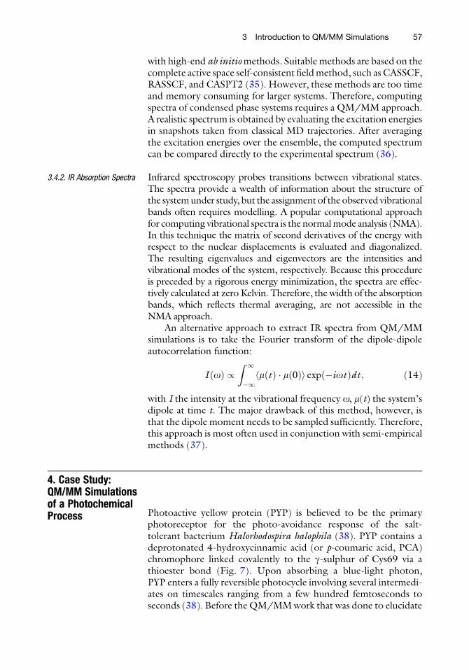
To examine the effect of an aqueous environment, we haveperformed 91 QM/MM excited-state dynamics simulations of achromophore analogue in water (39). The chromophore wasdescribed at the CASSCF(6,6)/3-21G level of theory, while thewater molecules were modelled by the SPC/E force field (40). Theresults of these simulations demonstrate that in water, radiationlessdecay is very efficient (39). The predominant excited-state decaychannel involves twisting of the single bond (88%) rather than thedouble bond (12%). In contrast to vacuum, decay takes place verynear these minima. Inspection of the trajectories revealed that decayis mediated by specific hydrogen bond interactions with watermolecules. These hydrogen bonds are different for the single-anddouble-twisted S1 minima, which reflects the difference in chargedistribution between these minima (41). In the single-bond twistedS1 minimum, the negative charge resides on the alkene moiety ofthe chromophore (Fig. 9). Three strong hydrogen bonds to thecarbonyl oxygen stabilize this charge distribution to such an extentthat the seam almost coincides with the single-bond twisted S1minimum (Fig. 10). In the double-bond twisted S1 minimum,the negative charge is localized on the phenolate ring (Fig. 9).Transient stabilization of this charge distribution by two or morestrong hydrogen bonds to the phenolate oxygen brings the seamvery close to this S1 minimum (Fig. 10). Thus, in water, the ultra-fast excited-state decay is mediated by hydrogen bonds.

4.4. Chromophore

in the Protein

To find out how the protein mediates the photochemical process,we also carried out a series of QM/MM simulations of wild-typePYP (42). Fig. 7 shows the primary events after photoexcitationin the simulation. The chromophore rapidly decays to the groundstate via a 90∘ rotation of the double bond (Fig. 7), rather thanthe single bond. During this photo-isomerization process, thehydrogen bonds between the chromophore’s phenolate oxygenatom and the side chains of the highly conserved Tyr42 and

Fig. 9. Excited-state minimum energy configurations of a chromophore analogue. In both the single-bond twisted S1minimum (a) and the double-bond twisted S1 minimum (b) there is a substantial energy gap between the ground andexcited state. The distribution of the negative charge in these minima is opposite.

60 G. Groenhof

Glu46 residues remain intact. Just as in water, these hydrogenbonds enhance excited-state decay from the double-bond twistedminimum.

Upon returning to the ground state, the chromophore eitherrelaxes back to the original trans conformation (180∘) or it con-tinues isomerizing to a cis conformation (0∘). In the latter case, therelaxation also involves a flip of the thioester linkage, which causesthe carbonyl group to rotate 180∘. During this rotation, the hydro-gen bond between the carbonyl oxygen and the Cys69 backboneamino group is broken (Fig. 7). In total, 14 MD simulations werecarried out, initiated from different snapshots from a classicalground-state trajectory. The fluorescence lifetime (200 fs) andisomerization quantum yield (30%) in the simulations agree wellwith experiments (400 fs (43) and 35% (38), respectively).

In the wild-type protein, no single-bond isomerization wasobserved. Thus, the protein not only provides the hydrogenbonds required for ultrafast decay but also controls which of thechromophore’s bonds isomerizes upon photoexcitation. We iden-tified the positive guanidinium moiety of Arg52 located just abovethe chromophore ring as the “catalytic” residue that enforcesdouble-bond isomerization. The preferential electrostatic stabiliza-tion of the double-bond twisted S1 minimum by the positive Arg52strongly favors double-bond isomerization over single-bondisomerization.

To elucidate the role of this arginine in the activation process inmore detail, we performed excited-state dynamics simulations onthe Arg52Gln mutant of PYP (44). This mutant can still enter thephotocycle, albeit with a lower rate and quantum yield (45, 46).Without the positive Arg52, the predominant excited-state reactionin the mutant involves isomerization of a single bond in the

Fig. 10. In water the chromophore undergoes both single-and double-bond isomerization. Excited-state decay from theseminima is very efficient due to stabilization of the chromophore’s S1 charge distribution by specific hydrogen bondinteractions.


chromophore, rather than the double bond (Fig. 11) (47). Thisobservation confirms that the role of Arg52 is to steer the initialevents after photoabsorption to ensure rotation of the doublerather than the single bond in the chromophore.

During the rotation of the single bond, the hydrogen bondbetween the carbonyl oxygen and Cys69 backbone amino group isbroken. As shown in Fig. 12, new hydrogen bonds are rapidlyformed between the carbonyl oxygen atom and the backboneamino groups of Tyr98 and Asp97. A water molecule from outsideenters the chromophore pocket to donate a third hydrogen bond.With these three hydrogen bonds stabilizing the negative charge onthe alkene moiety, the chromophore rapidly decays to S0. Thus, thedecay mechanism in the Arg52Gln mutant and in water are essen-tially the same.

Although single-bond isomerization does not result in the for-mation of the cis chromophore, a 180∘ flip of the thioester groupand a rupture of the hydrogen bond to Cys69 was observed with a20% quantum yield (Fig. 12). Together with the experimental

Fig. 12. Snapshots from an excited-state trajectory of the Arg52Gln mutant of PYP, demonstrating that three hydrogenbonds to the carbonyl moiety are essential for S1 decay at the single-bond twisted minimum. The first snapshot is at theexcitation to S1. The second snapshot shows the twisted configuration without hydrogen bonds to the carbonyl. The gapbetween S1 and S0 is far too high for decay at this configuration. However, the third snapshot shows two backbone aminogroups and a bulk water that has moved into the chromophore pocket during the excited-state dynamics, donating thethree hydrogen bonds that are required for efficient decay from the S1 minimum.

Fig. 11. Snapshots from an excited-state trajectory of the Arg52Gln mutant of PYP, showing the chromophore (pca) in theactive site pocket. The first snapshot is at the excitation. The second snapshot shows the configuration at the radiationlesstransition from S1 to S0. The third snapshot shows the photoproduct. In the mutant, isomerization takes place around thesingle bond. Like in the wild-type protein, the carbonyl oxygen of the thioester linkage flips, causing the break of thehydrogen bond to the backbone of Cys69.

62 G. Groenhof

observation that the mutant has a photoactivation quantum yield ofabout 21% (46), this suggests that the key step to enter the photo-cycle is the oxygen flip rather than the double-bond isomerization.

To summarize, the simulations are consistent with experimen-tal observations and have provided detailed structural and dynamicinformation at a resolution well beyond that achievable by othermeans. From the simulations, key amino acids have been identifiedand the mechanism by which they control the primary events in thephotocycle of PYP. These are (i) double-bond photoisomerization,and (ii) the break of a hydrogen bond between the chromophoreand the protein backbone. These events trigger a proton transferfrom the protein to the chromophore, which ultimately leads to thesignalling state of PYP (48).

5. Conclusionand Outlook

In this contribution we have reviewed the basic concepts of hybridQM/MM simulation techniques. More elaborate discussions onthe QM/MM method are available as review articles, see forinstance references (49–53). In principle, QM/MM simulationscan provide detailed structural information of chemical reactionsin the condensed phase at an atomic resolution. In practice, theQM/MM methods still suffer from limitations in computationalhardware, which restrict both system size and timescale of theprocesses that can be studied today. However, the expected increasein computer power, complemented by the development of moreefficient electronic structure methods and new algorithms maysoon enable the investigation of reactions in larger systems and atlonger timescales. Therefore, QM/MM simulation has the poten-tial to lead to a better understanding of chemical reactions, and themechanisms by which in particular protein environments controlthese reactions. Ultimately, these simulations may not only enableaccurate predictions of chemical properties but also become astandard tool for rational design of artificial molecular devices.

Acknowledgements

The Volkswagenstiftung and Deutsche Forschungsgemeinschaft(SFB755) are acknowledged for their financial support. I am grate-ful to Dr. Mehdi Davari and Pedro Valiente for critically reading themanuscript.


References

1. Jensen F (2001) Introduction to computa-tional chemistry. Wiley, New York

2. Berendsen HJC (2001) Bio-molecular dynam-ics comes of age. Science 271:954–955

3. McCammon JA, Gelin BR, Karplus M,Wolynes PG (1976) Hinge-bending mode inlysozyme. Nature 262:325–326

4. Shaw D,Maragakis P, Lindorff-Larsen K, PianaS, Dror R, Eastwood M, Bank J, Jumper J,Salmon J, Shan Y, Wriggers W, (2010)Atomic-level characterization of the structuraldynamics of proteins. Science 330:341–346

5. Warshel A, Levitt M (1976) Theoretical studiesof enzymatic reactions: dielectric, electrostaticand steric stabilization of carbonium ion in thereaction of lysozyme. J Mol Biol 103:227–249

6. Maseras F, Morokuma K (1995) IMOMM—anew integrated ab-initio plus molecularmechanics geometry optimization scheme ofequilibrium structures and transition-states.J Comput Chem 16:1170–1179

7. SvenssonM,Humbel S, Froese RDJ,MatsubaraT, Sieber S, Morokuma K (1996) ONIOM: amultilayered integrated MO + MM method forgeometry optimizations and single point energypredictions. A test for Diels–Alder reactions andPt(P(t-Bu)3)2 + H2 oxidative addition. J PhysChem 100:19357–19363

8. Bayly C, Cieplak P, Cornell W, Kollman P(1993) A well-behaved electrostatic potentialbsed method using charge restraints for deriv-ing atomic charges—the RESP model. J PhysChem 97:10269–10280

9. Besler B, Merz K, Kollman P (1990) Atomiccharges derived from semiempirical methods.J Comput Chem 11:431–439

10. Szabo A, Ostlund NS (1989) Modern quan-tum chemistry. Dover Publications, New York

11. Field MJ, Bash PA, Karplus M (1990) A com-bined quantum-mechanical and molecularmechanical potential for molecular-dynamicssimulations. J Comp Chem 11:700–733

12. Brooks B, Karplus M (1983) Harmonicdynamics of proteins—normal-modes and fluc-tuations in bovine pancreatic trypsin-inhibitor.Proc Natl Acad Sci USA 80:6571–6575

13. Dewar M (1983) Development and status ofMINDO/3 and MNDO. J Mol Struct100:41–50

14. Amara P, Field MJ (2003) Evaluation of an abinitio quantum mechanical/molecularmechanical hybrid-potential link-atommethod. Theor Chem Acc 109:43–52

15. Lamoureux G, Roux B (2003) Modelinginduced polarization with classical Drude oscil-lators: theory and molecular dynamics simula-tion algorithm. J Chem Phys 119:3025–3039

16. Warshel A, Sharma PK, Kato M, Xiang Y, LiuHB,OlssonMHM(2006) Electrostatic basis forenzyme catalysis. Chem Rev 106:3210–3235

17. Rappe AK, Goddard III WA (1991) Chargeequilibration for molecular dynamics simula-tions. J Phys Chem 95:3358–3363

18. Zhang Y, Lin H, Truhlar D (2007) Self-consistent polarization of the boundary in theredistributed charge and dipole scheme forcombined quantum-mechanical andmolecular-mechanical calculations. J ChemTheory Comput 3:1378–1398

19. Hillier I (1999) Chemical reactivity studied byhybrid QM/MM methods. J Mol Struct(Theochem) 463:45–52

20. Assfeld X, Rivail J (1996) Quantum chemicalcomputations on parts of large molecules: theab initio local self consistent field method.Chem Phys Lett 263:100–106

21. Gao J, Amara P, Alhambra C, FieldM (1998) Ageneralized hybrid orbital (GHO) method forthe treatment of boundary atoms in combinedQM/MM calculations. J Phys Chem A102:4714–4721

22. Philipp DM, Friesner RA (1999) Mixed abinitio QM/MM modeling using frozen orbi-tals and tests with alanine dipeptide and tetra-peptide. J Comput Chem 20:1468–1494

23. Nicoll R, Hindle S, MacKenzie G, Hillier I,Burton N (2001) Quantum mechanical/molecular mechanical methods and the studyof kinetic isotope effects: modelling the cova-lent junction region and application to theenzyme xylose isomerase. Theor Chem Acc106:105–112, 10th International Congress ofQuantum Chemistry, Nice, France, June13–15, 2000

24. Rodriguez A, Oliva C, Gonzalez M, van derKamp M, Mulholland A, (2007) Comparisonof different quantum mechanical/molecularmechanics boundary treatments in the reactionof the hepatitis C virus NS3 protease with theNS5A/5B substrate. J Phys Chem B111:12909–12915

25. Dewar MJS, Zoebisch EG, Healy EF, StewartJJP (1985) The development and use ofquantum-mechanical molecular modelsAM1—a new general-purpose quantum-mechanical molecular-model. J Am Chem Soc107:3902–3909

64 G. Groenhof

26. Stewart JJP (1989) Optimization of para-meters for semiempirical methods. 1. Method.J Comput Chem 10:209–220

27. Stewart JJP (1989) Optimization of para-meters for semiempirical methods. 2. Applica-tions. J Comput Chem 10:221–264

28. Elstner M, Porezag D, Jungnickel G, Elsner J,Haugk M, Frauenheim T, Suhai S, Seifert G(1998) Self-consistent-charge density-functional tight-binding method for simula-tions of complex materials properties. PhysRev B 58:7260–7268

29. Klahn M, Braun-Sand S, Rosta E, Warshel A(2005) On possible pitfalls in ab initio quan-tum mechanics/molecular mechanics minimi-zation approaches for studies of enzymaticreactions. J Phys Chem B 109:15645–15650

30. Torrie GM, Valle JP (1977) Non-physical sam-pling distributions in Monte-Carlo free energyestimation—umbrella sampling. J ComputPhys 23:187–199

31. Roux B (1995) The calculation of the potentialof mean force using computer-simulations.Comp Phys Comm 91:275–282

32. Kirkwood J (1935) Statistical Mechanics ofFluid Mixtures. J Chem Phys 3:300–313

33. Zwanzig R (1954) High-temperature equationof state by a perturbation method. I. Nonpolargases. J Chem Phys 22:1420–1426

34. Muller R, Warshel A (1995) Ab-initio calcula-tions of free energy barriers for chemical-reactions in solution. J Phys Chem99:17516–17524

35. Roos BO (1999) Theoretical studies of elec-tronically excited states of molecular systemsusing multiconfigurational perturbation the-ory. Acc Chem Res 32:137–144

36. Sch€afer LV, Groenhof G, Klingen AR, UllmannGM, Boggio-Pasqua M, Robb MA, Grubm€ul-ler H (2007) Photoswitching of the fluorescentprotein asFP595: mechanism proton pathways,and absorption spectra. Angew Chemie Int Ed46:530–536

37. Kaminski S, Gaus M, Phatak P, von Stetten D,Elstner M, Mroginski M (2010) VibrationalRaman spectra from the self-consistent chargedensity functional tight binding method viaclassical time-correlation functions. J ChemTheory Comput 6:1240–1255

38. Hellingwerf KJ, Hendriks J, Gensch T (2003)Photoactive yellow protein, a new type of pho-toreceptor protein: will this “yellow lab” bringus where we want to go? J Phys Chem A107:1082–1094

39. Boggio-Pasqua M, Robb M, Groenhof G(2009) Hydrogen bonding controls excited-

state decay of the photoactive yellow proteinchromophore. J Am Chem Soc 131:13580

40. Berendsen H, Grigera J, Straatsma T (1987)The missing term in effective pair potentials.J Phys Chem 91:6269–6271

41. Gromov EV, Burghardt I, Hynes JT, KoppelH, Cederbaum LS (2007) Electronic structureof the photoactive yellow protein chromo-phore: ab initio study of the low-lying excitedsinglet states. J Photochem Photobiol A190:241–257

42. Groenhof G, Bouxin-Cademartory M, Hess B,De Visser, S., Berendsen H, Olivucci M, MarkA, Robb M (2004) Photoactivation of thephotoactive yellow protein: why photonabsorption triggers a trans-to-cis lsomerizationof the chromophore in the protein. J AmChemSoc 126:4228–4233

43. Mataga N, Chosrowjan H, Shibata Y, ImamotoY, Tokunaga F (2000) Effects of modificationof protein nanospace structure and change oftemperature on the femtosecond to picosecondfluorescence dynamics of photoactive yellowprotein. J Phys Chem B 104:5191–5199

44. Shimizu N, Kamikubo H, Yamazaki Y, Ima-moto Y, kataoka M (2006) The crystal struc-ture of the R52Q mutant demonstrates a rolefor R52 in chromophore pK(a) regulation inphotoactive yellow protein. Biochemistry45:3542–3547

45. Changenet-Barret P, Plaza P, Martin MM,Chosrowjan H, Taniguchi S, Mataga N, Ima-moto Y, Kataoka M (2007) Role of arginine 52on the primary photoinduced events in the PYPphotocycle. Chem Phys Lett 434:320–325

46. Takeshita K, Imamoto Y, Kataoka M, Mihara K,Tokunaga F, Terazima M (2002) Structuralchange of site-directed mutants of PYP: newdynamics during pR state. Biophys J83:1567–1577

47. Groenhof G, Sch€afer LV, Boggio-Pasqua M,Grubm€uller H, Robb MA (2008) Arginine 52controls photoisomerization in photoactiveyellow protein. J Am Chem Soc in press JACS130: 3250–3251

48. Groenhof G, Lensink MF, Berendsen HJC,Mark AE (2002) Signal transduction in thephotoactive yellow protein. II. Proton transferinitiates conformational changes. Proteins48:212–219

49. Gao J (1996) Hybrid quantum and molecularmechanical simulations: an alternative avenueto solvent effects in organic chemistry. AccChem Res 29:298–305

50. Monard G, Merz K (1999) Combined quan-tum mechanical/molecular mechanical


methodologies applied to biomolecularsystems. Acc Chem Res 32:904–911

51. Gao J, Truhlar D (2002) Quantum mechanicalmethods for enzyme kinetics. Annu Rev PhysChem 53:467–505

52. Friesner R, Guallar V (2005) Ab initio quan-tum chemical and mixed quantum mechanics/

molecular mechanics (QM/MM) methods forstudying enzymatic catalysis. Annu Rev PhysChem 56:389–427

53. Senn H, Thiel W (2009) QM/MM methodsfor biomolecular systems. Angew Chem Int Ed48:1198–1229

66 G. Groenhof

Documents

Chapter 3 · Chapter 3 Introduction to QM/MM Simulations Gerrit Groenhof Abstract Hybrid quantum mechanics/molecular mechanics (QM/MM) simulations have become a popular tool for