1

CHAPTER 22

VALUING FIRMS WITH NEGATIVE EARNINGS

In most of the valuations thus far in this book, we have looked at firms that have

positive earnings. In this chapter, we consider a subset of firms with negative earnings or

abnormally low earnings that we categorize as troubled firms. We begin by looking at why

firms have negative earnings in the first place and look at the ways that valuation has to

be adapted to reflect these underlying reasons.

For firms with temporary problems – a strike or a product recall, for instance –

we argue that the adjustment process is a simple one, where we back out of current

earnings the portion of the expenses associated with the temporary problems. For

cyclical firms, where the negative earnings are due to a deterioration of the overall

economy, and for commodity firms, where cyclical movements in commodity prices can

affect earnings, we argue for the use of normalized earnings in valuation. For firms with

long-term strategic problems, operating problems – outdated plants, a poorly trained

workforce or poor investments in the past – or financial problems – too much debt – the

process of valuation becomes more complicated because we have to make assumptions

about whether the firm will be able to outlive its problems and restructure itself or

whether it will go bankrupt. Finally, we look at firms that have negative earnings because

they have borrowed too much and consider how best to deal with the potential for

default.

Negative Earnings: Consequences and Causes

A firm with negative earnings or abnormally low earnings is more difficult to value

than a firm with positive earnings. In this section, we look at why such firms create

problems for analysts in the first place and then follow up by examining the reasons for

negative earnings.

The Consequences of Negative or Abnormally Low Earnings

Firms that are losing money currently create several problems for the analysts who

are attempting to value them. While none of these problems are conceptual, they are

significant from a measurement standpoint.

2

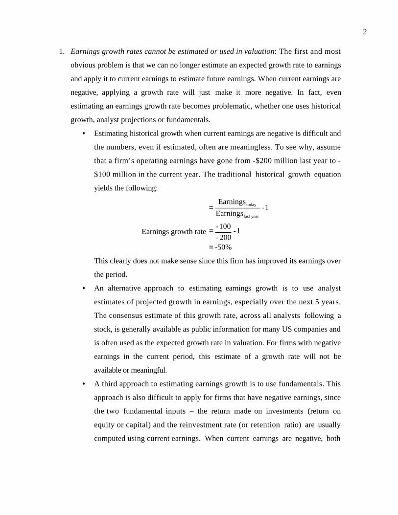
1. Earnings growth rates cannot be estimated or used in valuation: The first and most

obvious problem is that we can no longer estimate an expected growth rate to earnings

and apply it to current earnings to estimate future earnings. When current earnings are

negative, applying a growth rate will just make it more negative. In fact, even

estimating an earnings growth rate becomes problematic, whether one uses historical

growth, analyst projections or fundamentals.

• Estimating historical growth when current earnings are negative is difficult and

the numbers, even if estimated, often are meaningless. To see why, assume

that a firm’s operating earnings have gone from -$200 million last year to -

$100 million in the current year. The traditional historical growth equation

yields the following:

Earnings growth rate

-50%

1-200-

100-

1-Earnings

Earnings

yearlast

today

=

=

=

This clearly does not make sense since this firm has improved its earnings over

the period.

• An alternative approach to estimating earnings growth is to use analyst

estimates of projected growth in earnings, especially over the next 5 years.

The consensus estimate of this growth rate, across all analysts following a

stock, is generally available as public information for many US companies and

is often used as the expected growth rate in valuation. For firms with negative

earnings in the current period, this estimate of a growth rate will not be

available or meaningful.

• A third approach to estimating earnings growth is to use fundamentals. This

approach is also difficult to apply for firms that have negative earnings, since

the two fundamental inputs – the return made on investments (return on

equity or capital) and the reinvestment rate (or retention ratio) are usually

computed using current earnings. When current earnings are negative, both

3

these inputs become meaningless from the perspective of estimating expected

growth.

2. Tax computation becomes more complicated: The standard approach to estimating

taxes is to apply the marginal tax rate on the pre-tax operating income to arrive at the

after-tax operating income.

After-tax Operating Income = Pre-tax Operating Income (1 – tax rate)

This computation assumes that earnings create tax liabilities in the current period.

While this is generally true, firms that are losing money can carry these losses forward

in time and apply them to earnings in future periods. Thus, analysts valuing firms

with negative earnings have to keep track of the net operating losses of these firms

and remember to use them to shield income in future periods from taxes.

3. The Going Concern Assumption: The final problem associated with valuing companies

that have negative earnings is the very real possibility that these firms will go

bankrupt if earnings stay negative. And the assumption of infinite live that underlies

the estimation of terminal value may not apply in these cases.

The problems are less visible but exist nevertheless for firms that have abnormally

low earnings, i.e, the current earnings of the firm are much lower than what the firm has

earned historically. Though you can compute historical growth and fundamental growth

for these firms, they are likely to be meaningless because current earnings are depressed.

The historical growth rate in earnings will be negative and the fundamentals will yield

very low estimates for expected growth.

The Causes of Negative Earnings

There are several reasons why firms have negative or abnormally low earnings.

Some of which can be viewed as temporary, some of which are long term and some of

which relate to where a firm stands in the life cycle.

Temporary Problems

For some firms, negative earnings are the result of temporary problems,

sometimes affecting the firm alone, sometimes affecting an entire industry and sometimes

the result of a downturn in the economy.

4

• Firm-specific reasons for negative earnings can include a strike by the firm’s

employees, an expensive product recall or a large judgment against the firm in a

lawsuit. While these will undoubtedly lower earnings, the effect is likely to be

one-time and not affect future earnings.

• Sector-wide reasons for negative earnings can include a downturn in the price of a

commodity for a firm that produces that commodity. It is common, for instance,

for paper and pulp firms to go through cycles of high paper prices (and profits)

followed by low paper prices (and losses). In some cases, the negative earnings

may arise from the interruption of a common source of supply for a necessary

raw material or a spike in its price. For instance, an increase in oil prices will

negatively affect the profits of all airlines.

• For cyclical firms, a recession will affect revenues and earnings. It is not

surprising, therefore, that automobile companies report low or negative earnings

during bad economic times.

The common thread for all of these firms is that we expect earnings to recover sooner

rather than later as the problem dissipates. Thus, we would expect a cyclical firm’s

earnings to bounce back once the economy revives and an airline’s profits to improve

once oil prices level off.

Long Term Problems

Negative earnings are sometimes reflections of deeper and much more long-term

problems in a firm. Some of these are the results of poor strategic choices made in the

past, some reflect operational inefficiencies and some are purely financial, the result of a

firm borrowing much more than it can support with its existing cash flows.

• A firm’s earnings may be negative because its strategic choices in terms of product

mix or marketing policy might have backfired. For such a firm, financial health is

generally not around the corner and will require a substantial makeover and, often,

new management.

• A firm can have negative earnings because of inefficient operations. For instance,

the firm’s plant and equipment may be obsolete or its work force may be poorly

trained. The negative earnings may also reflect poor decisions made in the past by

5

management and the continuing costs associated with such decisions. For instance,

firms that have gone on acquisition binges and overpaid on a series of acquisitions

may face several years of poor earnings as a consequence.

• In some cases, a firm that is in good health operationally can end up with negative

equity earnings because it has chosen to use too much debt to fund its operations.

For instance, many of the firms that were involved in leveraged buyouts in the

1980s reported losses in the first few years after the buyouts.

Life Cycle

In some cases, a firm’s negative earnings may not be the result of problems in the

way it is run but because of where the firm is in its life cycle. We can think of at least

three examples.

• Firms in businesses that require huge infrastructure investments up front will often

lose money until these investments are in place. Once they are made and the firm is

able to generate revenues, the earnings will turn positive. You can argue that this was

the case with the phone companies in the early part of the twentieth century in the

United States, the cable companies in the 1980s and the cellular companies in the

early 1990s.

• Small biotechnology or pharmaceutical firms often spend millions of dollars on

research and come up with promising products that they patent, but then have to wait

years for FDA approval to sell the drugs. In the meantime, they continue to have

research and development expenses and report large losses.

• The third group includes young, start-up companies. Often these companies have

interesting and potentially profitable ideas, but they lose money until they convert

these ideas into commercial products. Until the late 1990s, these companies seldom

went public but relied instead of venture capital financing for their equity needs. One

of the striking features of the boom in new technology companies from 1997 to 2000

was the number of such firms that chose to bypass the venture capital route and go to

the markets directly.

Making the Call: Short term versus Long term Problems

6

In practice, it is often difficult to disentangle temporary or short-term problems

from long term ones. There is no simple rule of thumb that works and accounting

statements are not always forthcoming about the nature of the problems. Most firms,

when reporting negative earnings, will claim that their problems are transitory and that

recovery is around the corner. Analysts have to make their own judgments on whether

this is the case and they should consider the following.

- The credibility of the management making the claim: The managers of some firms are

much more forthcoming than others in revealing problems and admitting their

mistakes, and their claims should be given much more credence.

- The amount and timeliness of information provided with the claim: A firm that

provides detailed information backing up its claim that the problem is temporary is

more credible than a firm that does not provide such information. In addition, a firm

that reveals its problems promptly is more believable than one that delays reporting

problems until its hand is forced.

- Confirming reports from other companies in industry: A cyclical company that claims

that its earnings are down because of an economic slowdown will be more believable if

other companies in the sector also report similar slowdowns.

- The persistence of the problem: If poor earnings persist over multiple periods, it is

much more likely that the firm is facing a long-term problem. Thus, a series of

restructuring charges should be viewed with suspicion.

Valuing Negative Earnings Firms

The way we deal with negative earnings will depend upon why the firm has

negative earnings in the first place. In this section, we explore the alternatives that are

available for working with negative earnings firms.

Firms with temporary problems

When earnings are negative because of temporary or short-term problems, the

expectation is that earnings will recover in the near term. Thus, the solutions we devise

will be fairly simple ones, which for the most part will replace the current earnings (which

7

are negative) with normalized earnings (which will be positive). How we normalize

earnings will vary depending upon the nature of the problem.

Firm-Specific

A firm can have a bad year in terms of earnings, but the problems may be isolated

to that firm, and be short-term in nature. If the loss can be attributed to a specific event –

a strike or a lawsuit judgment, for instance – and the accounting statements report the

cost associated with the event, the solution is fairly simple. You should estimate the

earnings prior to these costs and use these earnings not only for estimating cash flows but

also for computing fundamentals such as return on capital. In making these estimates,

though, note that you should remove not just the expense but all of the tax benefits

created by the expense as well, assuming that it is tax deductible.

If the cause of the loss is more diffuse or if the cost of the event causing the loss is

not separated out from other expenses, you face a tougher task. First, you have to ensure

that the loss is in fact temporary and not the symptom of long term problems at the firm.

Next, you have to estimate the normal earnings of the firm. The simplest and most direct

way of doing this is to compare each expense item for the firm for the current year with

the same item in previous years, scaled to revenues. Any item that looks abnormally high,

relative to prior years, should be normalized (by using an average from previous years).

Alternatively, you could apply the operating margin that the firm earned in prior years to

the current year’s revenues and estimate an operating income to use in the valuation.

In general, you will have to consider making adjustments to the earnings of firms

after years in which they have made major acquisitions, since the accounting statements in

these years will be skewed by large items that are generally non-recurring and related to

the acquisition.

Illustration 22.1: Normalizing Earnings for a Firm after a Poor Year: Daimler Benz in

1995

In 1995, Daimler Benz reported an operating loss of DM 2,016 million and a net loss

of DM 5,674 million. Much of the loss could be attributed to firm-specific problems

including a large write off of a failed investment in Fokker Aerospace, an aircraft

manufacturer. To estimate normalized earnings at Daimler Benz, we eliminated all charges

8

related to these items and estimated a pre-tax operating income of DM 5,693 million. To

complete the valuation, we made the following additional assumptions.

• Revenues at Daimler had been growing 3-5% a year prior to 1995 and we anticipated

that the long term growth rate would be 5% in both revenues and operating income.

• The firm had a book value of capital invested of DM 43,558 million at the beginning

of 1995, and was expected to maintain its return on capital (based upon the adjusted

operating income of DM 5,693 million)

• The firm’s tax rate is 44%.1

To value Daimler, we first estimated the return on capital at the firm, using the adjusted

operating income.

Return on capital

( )

( )

%32.743558

44.015693

invested capital of Book value

t-1EBIT

=

−=

=

Based upon the expected growth rate of 5%, this would require a reinvestment rate of

68.31%.

Reinvestment rate %31.68%32.7

%5

ROC=== g

With these assumptions, we were able to compute Daimler’s expected free cash flows in

1996.

EBIT1995 (1+g) (1-t) = 5,693 (1.05) (1-0.44) = 3,347 Mil DM

- Reinvestment = 5,693 (1.05) (1-0.44) (0.6831)= 2,287 Mil DM

Free Cash Flow to Firm = 1,061 Mil DM

To compute the cost of capital, we used a bottom-up beta of 0.95, estimated using

automobile firms listed globally. The long-term bond rate (on a German government bond

denominated in DM) was 6%, and Daimler Benz could borrow long term at 6.1%. We

1 Germany has a particularly complicated tax structure since it has different tax rates for retained earningsand dividends, which makes the tax rate a function of a firm’s dividend policy.

9

assumed that a market risk premium of 4%. The market value of equity was 50,000

million DM, and there was 26,281 million DM in debt outstanding at the end of 1995.

Cost of Equity = 6%+ 0.95(4%)= 9.8%

Cost of Debt = 6.1%(1-.44) = 3.42%

Debt Ratio = 26,281/(50,000+26,281) = 34.45%

Cost of Capital = 9.8%(.6555) + 3.42% (.3445) = 7.60%

Note that all of the costs are computed in DM terms to be consistent with our cash

flows. The firm value can now be computed, if we assume that earnings and cash flows

will grow at 5% a year in perpetuity.

Value of the operating assets

DMmillion 40,787

0.05-0.076

1061

g-capital ofCost

FCFF

rategrowth Expected-capital ofCost

1996in FCFF Expected

1996

=

=

=

=

Adding to this the value of the cash and marketable securities (13,500 million DM) held

by Daimler at the time of this valuation and netting out the market value of debt yields an

estimated value of 28,006 million for equity, significantly lower than the market value of

50,000 million DM.

Value of equity = Value of operating assets + Cash and Marketable securities – Debt

= 40787+13500 – 26281 = 28,006 million DM

As in all firm valuations, there is an element of circular reasoning2 involved in this

valuation.

Sector Wide or Market Driven Problems

The earnings of cyclical firms are, by definition, volatile and dependent upon the

state of the economy. In economic booms, the earnings of these firms are likely to

increase, while, in recessions, the earnings will be depressed. The same can be said of

2 The circular reasoning comes in because we use the current market value of equity and debt to computethe cost of capital. We then use the cost of capital to estimate the value of equity and debt. If this is

10

commodity firms that go through price cycles, where periods of high prices for the

commodity are often followed by low prices. In both cases, you can get misleading

estimates of value if you use the current year’s earnings.

Valuing Cyclical Firms

In most discounted cashflow valuations, the current year is used as the base year

and growth rates are used to project future earnings and cashflows. Depending upon what

stage of the economic cycle a valuation is done at, the current year's earnings may be too

low (if you are in a recession) or too high (if the economy is at a peak) to use as a base

year. The failure to adjust the base year's earnings for cyclical effects can lead to

significant errors in valuation, since the earnings are likely to adjust as the economic cycle

changes. There are two potential solutions – one is to adjust the expected growth rate in

the near periods to reflect cyclical changes and the other is to value the firm based upon

normalized rather than current earnings.

a. Adjust Expected Growth

Cyclical firms often report low earnings at the bottom of an economic cycle, but the

earnings recover quickly when the economy recovers. One solution, if earnings are not

negative, is to adjust the expected growth rate in earnings, especially in the near term, to

reflect expected changes in the economic cycle. This would imply using a higher growth

rate in the next year or two, if both the firm’s earnings and the economy are depressed

currently but are expected to recover quickly. The strategy would be reversed if the

current earnings are inflated (because of an economic boom) and if the economy is

expected to slow down. The disadvantage of this approach is that it ties the accuracy of

the estimate of value for a cyclical firm to the precision of the macro-economic

predictions of the analyst doing the valuation. The criticism, though, may not be

avoidable since it is difficult to value a cyclical firm without making assumptions about

future economic growth. The actual growth rate in earnings in 'turning-point' years (years

unacceptable, the process can be iterated, with the cost of capital being recomputed using the estimatedvalues of debt and equity and continued until there is convergence.

11

when the economy goes into or comes out of a recession) can be estimated by looking at

the experience of this firm (or similar firms) in prior recessions.

Illustration 22.2: Valuing a cyclical firm during a recession – adjusting the growth rate:

Chesapeake Corp. in early 1993

Chesapeake Corporation, which makes recycled commercial and industrial tissue,

is a cyclical firm in the paper products industry, had earnings per share in1992 of $0.63,

down from $2.51 in 1988. If the 1992 earnings per share had been used as the base year's

earnings, Chesapeake Corporation would be valued based upon the following inputs.

Current earnings per share = $ 0.63

Current depreciation per share = $ 2.93

Current capital spending per share = $3.63

Debt Ratio for financing capital spending = 45%

Chesapeake had a beta of 1.00 and no significant working capital requirements. The

treasury bond rate was 8.5% at the time of this analysis and the risk premium of 4% for

stocks over bonds is used.

Cost of equity = 8.5% + 1 (4%) = 12.5%

If we valued Chesapeake based upon current earnings and assume a long-term growth rate

of 6%, we would have estimated a value per share of $ 4.00.

Free Cashflow to Equity in 1992 = $ 0.63 - (1-0.45) ($3.63 - $2.93) = $0.245

Value per share ( )( )

$4.000.06-0.125

1.06$0.245 ==

Chesapeake Corp. was trading at $20 per share in May 1993.

Assume that the economy is expected to recover slowly in 1993 and much faster

in 1994. As a consequence, the growth rates in earnings projected for Chesapeake

Corporation are as follows.

Year Expected Growth RateEarnings per share

1993 5% $ 0.66

1994 100% $ 1.32

1995 50% $ 1.98

After 1996 6%

12

The capital spending and depreciation are expected to grow at 6%. The free cashflow to

equity can be estimated as follows.

1993 1994 1995 1996

EPS $0.66 $1.32 $1.98 $2.10

- (Cap Ex - Deprecn) ( 1- Debt Ratio) $0.41 $0.43 $0.46 $0.49

= FCFE $0.25 $0.89 $1.53 $1.62

Terminal price (at the end of 1995) $24.880.06- 0.125

$1.62 ==

Present Value per share =0.25

1.125+

0.89

1.1252 +1.53 + 24.88

1.1253 =19.47

b. Normalize Earnings

For cyclical firms, the easiest solution to the problem of volatile earnings over time

and negative earnings in the base period is to normalize earnings. When normalizing

earnings for a firm with negative earnings, we are simply trying to answer the question:

“What would this firm earn in a normal year?” Implicit in this statement is the

assumption that the current year is not a normal year and that earnings will recover

quickly to normal levels. This approach, therefore, is most appropriate for cyclical firms

in mature businesses. There are a number of ways in which earnings can be normalized.

• Average the firm’s dollar earnings over prior periods: The simplest way to

normalize earnings is to use the average earnings over prior periods. How many

periods should you go back in time? For cyclical firms, you should go back long

enough to cover an entire economic cycle – between 5 and 10 years. While this

approach is simple, it is best suited for firms that have not changed in scale (or

size) over the period. If it is applied to a firm that has become larger or smaller (in

terms of the number of units it sells or total revenues) over time, it will result in a

normalized estimate that is incorrect.

• Average the firm’s return on investment or profit margins over prior periods: This

approach is similar to the first one, but the averaging is done on scaled earnings

instead of dollar earnings. The advantage of the approach is that it allows the

normalized earnings estimate to reflect the current size of the firm. Thus, a firm

13

with an average return on capital of 12% over prior periods and a current capital

invested of $1,000 million would have normalized operating income of $120

million. Using average return on equity and book value of equity yields normalized

net income. A close variant of this approach is to estimate the average operating or

net margin in prior periods and apply this margin to current revenues to arrive at

normalized operating or net income. The advantage of working with revenues is

that they are less susceptible to manipulation by accountants.

There is one final question that we have to deal with when normalizing earnings and it

relates to when earnings will be normalized. Replacing current earnings with normalized

earnings essentially is equivalent to assuming that normalization will occur

instantaneously (i.e., in the very first time period of the valuation). If earnings will be

normalized over several periods, the value obtained by normalizing current earnings will

be too high. A simple correction that can be applied is to discount the value back by the

number of periods it will take to normalize earnings.

Illustration 22.3: Normalizing Earnings for a Cyclical Firm in a Recession: Historical

Margin

In 1992, towards the end of a recession in Europe and the United States, Volvo

reported an operating loss of 2,249 million Swedish Kroner (Sk) on revenues of 83,002

million Sk. To value the firm, we first had to normalize earnings. We used Volvo’s average

pre-tax operating margin from 1988 to 1992 of 4.1% as a measure of the normal margin

and applied it to revenues in 1992 to estimate normalized operating income.

Normalized operating income in 1992

( )( )( )( )

Skmillion 403,3

041.0002,83

\Margin Normalized92Revenues19

===

To value the operating assets of the firm, we assumed that Volvo was in stable growth, a

reasonable assumption given its size and the competitive nature of the automobile

industry, and that the expected growth rate in perpetuity would be 4%. To estimate the

firm’s reinvestment needs, we assumed that Volvo’s return on capital in the future would

be equal to the average return on capital that the firm earned between 1988 and 1992,

14

which was 12.2%. This allowed use to estimate a reinvestment rate for the firm of

32.78%.

Reinvestment rate in stable growth 32.78%ROC

4%

ROC

g ===

The expected free cash flow to the firm in 1993, based upon the normalized pre-tax

operating income of 3,403 million Sk, an estimated tax rate of 35%, the expected growth

rate of 4% and the reinvestment rate of 32.78% can be estimated.

Expected free cash flow to the firm in 1993

= 3403 (1.04) (1-.35) (1 - .3278) = 1,546 million Sk

To estimate the cost of capital for Volvo, we computed weights upon the market value of

equity of 22,847 million Sk at the end of 1992 and the debt outstanding of 42641 million

Sk. We used a bottom-up beta of 1.20 for Volvo and a pre-tax cost of debt of 8.00%,

reflecting its high leverage at the time of the analysis. The riskfree rate in Swedish kroner

was 6.6% and the risk premium used was 4%:

Cost of equity = 6.6% + 1.2 (4%) = 11.40%

Cost of capital = 11.40%( ) 22847

22847 + 42641

+ 8%( ) 1−0.35( ) 42641

22847 + 42641

= 7.36%

The value of the operating assets of Volvo can now be estimated.

Value of operating assets

= Expected FCFF in 1993

Cost of capital -Expected growth

=1546

0.0736 − 0.04= 45,977 million Sk

Adding to this the value of cash and marketable securities (20,760 million Sk) held by the

firm at the end of 1992 and subtracting out debt yields an estimated value for equity.

Value of equity = Value of operating assets + Cash & marketable securities – Debt

= 45977 + 20760 – 42641 = 24,096 million Sk

Based upon this estimate, Volvo was slightly undervalued at the end of 1992.

Implicitly, we are assuming that Volvo’s earnings will rebound quickly to

normalized levels and that the recession will end in the very near future. If we assume that

the recovery will take time, we can incorporate the effect into value by discounting the

15

value estimated in the analysis above back by the number of years that it will take Volvo

to return to normal earnings. For instance, if we assume that adjustment will take 2 years,

we could discount the value of the firm back two years at the cost of capital and then add

cash and subtract out the debt outstanding:

Value of the operating assets assuming 2-year recovery = 45977/1.07362 = 39,889

+ Cash and marketable securities + 20,760

- Value of Debt outstanding - 42641

= Value of Equity =18,008

If we assume that the recovery will take two years or more, Volvo’s equity is overvalued.

normearn.xls: This spreadsheet allows you to normalize the earnings for a firm,

using a variety of approaches.

Macro-economic views and Valuation

The earnings of cyclical firms tend to be volatile, with the volatility linked to how

well or badly the economy is performing. One way to incorporate these effects into value

is to build in expectations of when future recessions and recoveries will occur into the

cashflows. This exercise is fraught with danger, since the error in such predictions is likely

to be very large. Economists seldom agree on when a recovery is imminent, and most

categorizations of recessions occur after the fact. Furthermore, a valuation that is based

upon specific macro-economic forecasts makes it difficult for users to separate how much

of the final recommendation, i.e. that the firm is under or over valued, comes from the firm

being mis-priced and how much reflects the analyst’s optimism or the pessimism about

the overall economy.

The other way to incorporate earnings variability into the valuation is through the

discount rate - cyclical firms tend to be more risky and require higher discount rates. This

is what we do when we use higher unlevered betas and/or costs of debt for cyclical firms.

Valuing Commodity and Natural Resource Firms

Commodity prices are not only volatile but go through cycles – periods of high

prices followed by periods with lower prices. Figure 22.1 summarizes the levels of three

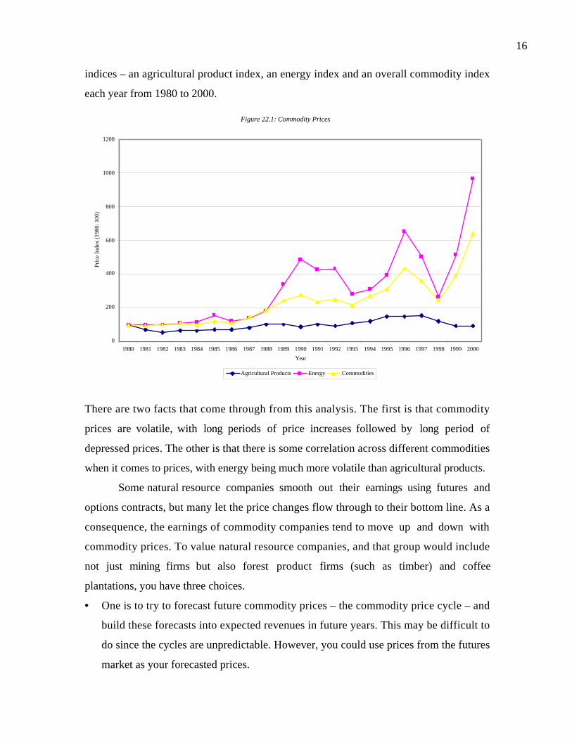
16

indices – an agricultural product index, an energy index and an overall commodity index

each year from 1980 to 2000.

There are two facts that come through from this analysis. The first is that commodity

prices are volatile, with long periods of price increases followed by long period of

depressed prices. The other is that there is some correlation across different commodities

when it comes to prices, with energy being much more volatile than agricultural products.

Some natural resource companies smooth out their earnings using futures and

options contracts, but many let the price changes flow through to their bottom line. As a

consequence, the earnings of commodity companies tend to move up and down with

commodity prices. To value natural resource companies, and that group would include

not just mining firms but also forest product firms (such as timber) and coffee

plantations, you have three choices.

• One is to try to forecast future commodity prices – the commodity price cycle – and

build these forecasts into expected revenues in future years. This may be difficult to

do since the cycles are unpredictable. However, you could use prices from the futures

market as your forecasted prices.

Figure 22.1: Commodity Prices

0

200

400

600

800

1000

1200

1980 1981 1982 1983 1984 1985 1986 1987 1988 1989 1990 1991 1992 1993 1994 1995 1996 1997 1998 1999 2000

Year

Pric

e In

dex

(198

0: 1

00)

Agricultural Products Energy Commodities

17

• You could value the firms using a normalized commodity price, estimated by looking

at the average price of the commodity over a cycle. Thus, the average price of coffee

over the last decade can be used to estimate the value of a coffee plantation. The

danger, of course, is that the price of coffee may stay well above or below this average

price for an extended period, throwing off estimates of value.

• You could value the firm’s current production using the current price for the

commodity, low though it might be, and add to it the value of the option that the

company possesses, which is to produce more if prices go up and less if they go

down. We will look at this approach in more detail in Chapter 28.

Illustration 22.4: Valuing a Commodity company: Aracruz Celulose

Aracruz Celulose is a Brazilian paper and pulp manufacturer and, like all firms in

this sector, it is susceptible to the ups and downs of the price of paper and pulp. In

Figure 22.2, we report on the revenues and operating income at Aracruz over the last

decade and, in the same graph, we provide an index of the price of paper and pulp each

year.

18

Note the correlation between Aracruz’s fortunes and the price of paper and pulp. The

years with low or negative earnings for Aracruz generally are also the years when paper

prices decline.

In May 2001, when we valued Aracruz, the firm had just emerged from a year of

high paper prices and profitability to report 666 million BR of operating income on

revenues of 1,342 million BR in 2000; the firm faced a tax rate of 33%. If we use this

operating income to value Aracruz, we are assuming that paper prices will continue to

remain high. To prevent this from biasing the valuation, we re-estimated revenues and

operating income in 2000, using the average price of paper over the last decade.

Restated revenues = Revenues2000*(Average Paper Price91-00/Paper

= 1342 * (102.58/109.39) = 1258 million BR

Restated operating income = Restated revenues – Operating expenses

= 1258 - (1342-666) = 582 million BR

This operating income was used to compute a normalized return on capital for the firm of

10.55%, based upon the book values of debt ($1549 million) and equity ($2149 million)

invested at the end of the previous year:

Figure 22.2: Aracruz Celulose: Revenues, Profits and the Price of Paper

-$200.00

$0.00

$200.00

$400.00

$600.00

$800.00

$1,000.00

$1,200.00

$1,400.00

$1,600.00

1991 1992 1993 1994 1995 1996 1997 1998 1999 2000

Year

Rev

enue

s &

Ope

ratin

g In

com

e

80

85

90

95

100

105

110

115

Pric

e of

pap

er (

1992

: 100

)

RevenuesOperating IncomePrice of pulp

19

Normalized Return on capital

=Operating Income 2000 1-t( )

Book value of debt 1999 + Book value of equity 1999

=582 1−0.33( )1549 + 2149

=10.55%

We assumed that the firm would maintain this return on capital and grow 10% a year, in

real terms, for the next 5 years and 3% a year in real terms in perpetuity after that. Table

22.1 summarizes projections of free cash flows to the firm for Aracruz for the next 5

years and for the first year of stable growth (6 years from now).

Table 22.1: Operating Income and Expected Free Cashflows to the Firm

1 2 3 4 5

Terminal

year

Expected Growth 10% 10% 10% 10% 10% 3%

Reinvestment rate 94.79% 94.79% 94.79% 94.79% 94.79% 28.44%

EBIT $644 $712 $787 $870 $961 $1,063

EBIT (1-t) $431 $477 $527 $583 $644 $712

- Reinvestment $409 $452 $500 $552 $611 $203

= FCFF $22 $25 $27 $30 $34 $510

Note that the reinvestment rate each year is computed based upon the expected growth

rate and return on capital,

Reinvestment rate capitalon return Normalized

g=

As expected growth declines in year 6 (the terminal year), the reinvestment rate also

declines.

The cost of capital was estimated in real terms, using a bottom-up beta of 0.70

estimated by looking at paper and pulp firms and an additional risk premium for exposure

to Brazilian country risk – 10.24% for the next 5 years and 5% after 5 years. This is in

addition to the equity risk premium of 4%. We use a real riskfree rate of 4%: To estimate

20

the real cost of debt, we assume a pre-tax real cost of borrowing of 7.5% for Aracruz for

both the high growth and stable growth periods.

Real after-tax cost of debt = 7.5% (1-0.33) = 5.03%

The current market values of equity (3749 million BR) and debt (1395 million BR) were

used to compute a market debt to capital ratio of 27.11% and the costs of capital for both

periods are shown in Table 22.2.

Table 22.2; Costs of capital – High Growth and Stable growth periods

High Growth Stable Growth

Beta 0.7 0.7

Riskfree Rate 4% 4%

Mature Market Premium 4% 4%

Country premium 10.24% 5%

Cost of equity = 4%+0.7(4%+10.24%) =13.97%4%+0.7(4%+5%) =10.30%

Cost of debt = 5.03% 5.03%

Debt ratio = 27.11% 27.11%

Cost of capital = 11.54% 8.87%

The terminal value is first estimated using the terminal year’s cash flows estimated in

Table 22.1 and the perpetual growth rate of 3%.

Terminal value = FCFFTerminal year/ (Cost of capitalstable – g)

= 510/(.0887- .03) = 8,682 million BR

The value of the operating assets of firm can be computed today as the present value of

the cash flows for the next 5 years and the present value of the terminal value, using the

high growth period cost of capital as the discount rate:

Value of operating assets = 22/1.1154 + 25/1.11542+ 27/1.11543+ 30/1.11544+

34/1.11545+ 8682/1.11545 = 5,127 million BR

We added back the value of cash and marketable securities (849 million BR) and

subtracted outstanding debt (1395 million) to estimate a value of equity:

Value of equity = 5127 + 849 – 1395 = 4,581 million BR

This would suggest that the firm is under valued at its current value of 2,149 million BR.

Multiples and Normalized Earnings

21

Would you have to make these adjustments to earnings if you were doing relative

valuation rather than discounted cash flow valuation? The answer is generally yes and

when adjustments are not made, you are implicitly assuming normalization of earnings.

To see why, assume that you are comparing steel companies using price earnings

ratios and that one of the firms in your group has just reported very low earnings because

of a strike during the last year. If you do not normalize the earnings, this firm will look

over valued relative to the sector, because the market price will probably be based upon

the expectation that the labor troubles, though costly, are in the past. If you use a

multiple such as price to sales to make your relative valuation judgments and you

compare this firm’s price to sales ratio to the industry average, you are assuming that the

firm’s margins will converge on industry averages sooner rather than later.

What if an entire sector’s earnings are affected by an event? Would you still need

to normalize? We believe so. Though the earnings of all automobile stocks may be

affected by a recession, the degree to which they are affected can vary widely depending

upon differences in operating and financial leverage. Furthermore, you will find yourself

unable to compute multiples such as price earnings ratios for many of the firms in the

group that lose money during recessions. Using normalized earnings will yield multiples

that are more reliable measures of true value.

Firms with long-term problems

In all of the valuations that we presented in the last section, we adjusted earnings

either instantaneously to reflect normal levels or very quickly, reflecting our belief that

the negative earnings will soon pass. In some cases, though, the negative earnings are a

manifestation of more long-term problems at the firm. In such cases, we will be forced to

make judgments on whether the problem will be overcome and, if so, when this will occur.

In this section, we present a range of solutions for companies in this position.

Strategic Problems

Firms can sometimes make mistakes in terms of the product mix they offer, the

marketing strategies they adopt or even the markets that they choose to target. They

22

often end up paying a substantial cost in terms of negative or lower earnings and perhaps

a permanent loss of market share. Consider the following examples.

• IBM found its dominant position in the mainframe computer business and the

extraordinary profitability of that business challenged by the explosion of the

personal computer market in the 1980s. While IBM could have developed the

operating system for personal computers early in the process, it ceded that

business to an upstart called Microsoft. By 1989, IBM had lost more than half its

market value and its return on equity had dropped into the single digits.3

• For decades, Xerox dominated the copier business to the extent that its name

became synonymous with the product. In the 1970s and 1980s, it was challenged

by Asian firms, with lower cost structures, like Ricoh and Canon for the market.

After initial losses, Xerox was able to recoup some of its market share. However

the last part of the 1990s saw a steady decline in Xerox’s fortunes as technology

(in the form of emails, faxes and low cost printers) took its toll. By the end of

2000, there were questions about whether Xerox had a future.

• Under the leadership of Michael Armstrong, AT&T tried to shed its image as a

stodgy phone company and became a technology firm. After some initial

successes, a series of miscues and poor acquisitions saw the firm enter the new

millennium with a vastly reduced market capitalization and no clear vision on

where to go next.

When firms have low or negative earnings that can be traced to strategic missteps, you

have to determine whether the shift is a permanent one. If it is, you will have to value the

firm on the assumption that it will never recover lost ground and scale down your

expectations of revenue growth and expected margins. If, on the other hand, you are more

optimistic about the firm’s recovery or its entry into new markets, you can assume that

the firm will be able to revert back to its traditional margins and high growth.

Operating Problems

3 It is worth noting that IBM made a fulsome recovery in the following decades by going back to basics,cutting costs and refocusing its efforts on business services.

23

Firms that are less efficient in the delivery of goods and services than their

competitors will also be less profitable and less valuable. But how and why do firms

become less efficient? In some cases, it can be traced to a failure to keep up with the times

and replenish existing assets and keep up with the latest technology. A steel company

whose factories are decades old and whose equipment is outdated will generally bear

higher costs for every ton of steel that it produces than its newer competitors. In other

cases, the problem may be labor costs. A steel company with plants in the United States

faces much higher labor costs than a similar company in Asia.

The variable that best measures operating efficiency is the operating margin, with

firms that have operating problems tending to have much lower margins than their

competitors. One way to build in the effect of operating improvements over time is to

increase the margin towards the industry average, but the speed with which the margins

will converge will depend upon several factors.

- Size of the firm: Generally, the larger the firm, the longer it will take to eliminate

inefficiencies. Not only is inertia a much stronger force in large firms, but the absolute

magnitude of the changes that have to be made are much larger. A firm with $10 billion

in revenues will have to cut costs by $300 million to achieve a 3% improvement in

pre-tax operating margin, whereas a firm with $100 million in revenues will have to

cut costs by $3 million to accomplish the same objective.

- Nature of the inefficiency: Some inefficiencies can be fixed far more quickly than

others. For instance, a firm can replace outdated equipment or a poor inventory

system quickly, but retraining a labor force will take much more time.

- External constraints: Firms are often restricted in terms of how much and how quickly

they can move to fix inefficiencies by contractual obligations and social pressure. For

instance, laying off a large portion of the work force may seem to obvious solution for

a firm that is overstaffed, but union contracts and the potential for negative publicity

may make firms reluctant to do so.

- Management Quality: A management that is committed to change is a critical

component of a successful turnaround. In some cases, a replacement of top

management may be necessary for a firm to resolve its operating problems.

24

Illustration 22.5: Valuing a firm with operating problems: Marks and Spencer

Marks and Spencer, a multinational retailer headquartered in the U.K, saw is

operating income halved from 1996 to 2000, partly because of a high cost structure and

partly because of ill-conceived expansion. In 2000, the firm reported £552 million in

operating income on revenues of £8,196 million - a pre-tax operating margin of 6.73%. In

contrast, the average operating margin for department stores in the U.K. and U.S. is 12%

and Market and Spencer’s own historical margin (over the previous decade) is 11%. To

value Marks and Spencer, we will assume the following.

- Revenues will grow 5% a year in perpetuity. The firm is a large firm in a mature

market and it does seem unrealistic to assume much higher growth in revenues.

- The firm reported capital expenditures of £448 million and depreciation of £262

million for the 2000 financial year. In addition, the non-cash working capital at the end

of the year was £1948 million. We will assume that net capital expenditures and non-

cash working capital will continue to grow at the same rate as revenues, i.e., 5% a year

forever.

- We will assume that the pre-tax operating margin of the firm will improve over the

next 10 years from 6.73% to 11.50%, with more significant improvements occurring

in the next 2 years and smaller improvements thereafter.

- We will use a tax rate of 33% to estimate after-tax cash flows. The cost of capital for

the firm is estimated using its current market debt to capital ratio of 20%, a cost of

equity of 9.52% and a pre-tax cost of debt of 6%.

Cost of capital = 9.52% (0.80) + 6% (1-0.33) (0.2) = 8.42%

Table 22.3 summarizes the forecasts of revenues, operating income and free cash flows to

the firm every year for the next 6 years.

Table 22.3: Forecasts of free cash flow to the firm

Year Revenues

Operating

Margin EBIT EBIT(1-t)Net Cap Ex

Change in

Working Capital FCFF

Current $8,196 6.73% $552 $370 $186

1 $8,606 8.32% $716 $480 $195 $97 $187

2 $9,036 9.38% $848 $568 $205 $102 $261

25

3 $9,488 10.09% $957 $641 $215 $107 $319

4 $9,962 10.56% $1,052 $705 $226 $113 $366

5 $10,460 10.87% $1,137 $762 $237 $118 $406

6 $10,983 11.08% $1,217 $815 $249 $124 $442

7 $11,533 11.22% $1,294 $867 $262 $131 $475

8 $12,109 11.31% $1,370 $918 $275 $137 $506

9 $12,715 11.38% $1,446 $969 $289 $144 $537

10 $13,350 11.42% $1,524 $1,021 $303 $151 $567

Term

year $14,018 11.50% $1,612 $1,080

After year 10, we assume that revenues and operating income will continue to grow 5% a

year forever, and that Marks and Spencer will earn an industry average return on capital

of 15%. This allows us to estimate a stable period reinvestment rate and terminal value.

Reinvestment rate in stable growth 33.33%15%

5%

ROC

g ===

Terminal value

( )( )

( )

million 054,21£05.00842.0

3333.011080

g-capital ofCost

ratent Reinvestme-1t-1EBIT11

=−

−=

=

Adding the present value of the cash flows in Table 22.3 to the present value of the

terminal value, using the cost of capital of 8.42% as the discount rate, yields a value for

the operating assets of £11,879 million. Adding the value of cash and marketable

securities at the end of 2000 to this amount and subtracting out the debt yields a value of

equity of £10,612 million.

Value of operating assets = £11,879 million

+ Cash & Securities = £687 million

- Debt = £1,954 million

Value of equity = £10,612 million

Dividing by the 2875 million shares outstanding yields a value per share of £3.69, higher

than the stock price of £2.72 prevailing at the time of this analysis in May 2001.

26

The Special Case of Privatizations

In many privatizations, we are called upon to value firms with long financial

histories but not very profitable ones. The lack of profitability is not surprising, however,

since many of these firms have been run with objectives other than maximizing value or

profitability. In some cases, employment in these firms has been viewed as a source of

political patronage. Consequently, they end up over-staffed and inefficient.

Will this all change as soon as they are privatized? Not necessarily, and certainly

not immediately. The power of unions to preserve existing jobs, the power that

governments continue to have on how they are run and the sheer size of these firms

makes change both daunting and slow. While it is reasonable to assume that these firms

will, in fact, become more efficient once they are privatized, the speed of the

improvement will vary from firm to firm. In general, you would expect the adjustment to

be much quicker if the government relinquishes its power to control the management of

the firm and if there are strong competitive pressures to become more efficient. It will be

slower if the firm is a monopoly and the government continues to handpick the top

management of the firm.

Illustration 22.6: Valuing a privatization – CVRD

In 1995, the Brazilian government privatized Compahnia Vale Dio Roce (CVRD),

Latin America’s biggest mining company. In the year the firm was privatized, it reported

after-tax operating income of 717 million BR on revenues of 4714 million BR. Based on

the capital invested in the firm at the beginning of the year of 14,722 million BR, the

after-tax return on capital earned by the firm was 5.33%.

If we assumed a stable real growth rate of 3% and a real cost of capital of 10%,

and valued CVRD on the basis of these inputs, we would have estimated the following

value for the firm.

Reinvestment rate 56.29%5.33%

3%

ROC

g ===

27

Value of the firm

( )( )( )

( )( )( )

BRmillion 611,403.010.0

5629.0103.1717

g-capital ofCost

ratent Reinvestme-11t-1EBIT

=−

−=

+= g

Note, though, that this assumes that CVRD’s return on capital will remain at existing

levels in perpetuity. If privatization leads to operating efficiencies at the firm, its margins

and return on capital can be expected to improve. For instance, if we valued CVRD using

the real return on capital of 7% earned by mining companies in the United States, we

would have estimated the following.

Reinvestment rate %86.247%

3%

ROC

g ===

Value of the firm

( )( )( )

( )( )( )

BRmillion 029,603.010.0

4286.0103.1717

g-capital ofCost

ratent Reinvestme-11t-1EBIT

=−

−=

+= g

Is it reasonable to assume this improvement in margins? It depends upon which

side of the transaction you are on. If you were an investor interested in buying the stock,

you might argue that the firm is too entrenched in its ways to make the changes needed

for higher profitability and use the value estimated with current margins. If you are the

government and want to obtain the highest value you can, you would argue for the latter.

Golden Shares and the Value of Privatized firms

While governments are always eager to receive the cash proceeds from privatizing

the firms that they own, they are generally not as eager to give up control of these firms.

One way they attempt to preserve power is by maintaining what is called a golden share

in the firm that gives them veto power and control over some or many aspects of the

firm’s management.

For instance, the Brazilian government maintains a golden share in CVRD,

allowing it the final decision on whether mines can be closed and other major financial

decisions. While governments often view these golden shares as a costless way to

privatize and preserve control at the same time, there is a cost that they will bear.

28

Investors valuing firms with golden shares will generally be much less willing to assume

radical changes in management and improvements in efficiency. Consequently, the values

attached to these firms by the market will be much lower. The more inefficient the firm

being privatized and the more restrictive the golden share, the greater will be the loss in

value to the government.

Financial Leverage

In some cases firms get into trouble because they borrow too much and not

because of operating or strategic problems. In these cases, it will be the equity earnings

that will be negative while operating earnings will be positive. The solution to the

problem depends, in large part, on how distressed the firm really is. If the distress is not

expected to push the firm into bankruptcy, there are a variety of potential solutions. If on

the other hand, the distress is likely to be terminal, finding a solution is much more

difficult.

Overlevered with no immediate threat of bankruptcy

Firms that borrow too much are not always on the verge of bankruptcy. In fact,

firms with valuable operating assets and substantial operating cash flows can service

much more debt than is optimal for them, even though they might not do so comfortably.

So, what are the costs of being overlevered? First, the firm might end up with a large

enough exposure to default risk that it affects its operations – customers might not buy

its products, suppliers might demand speedier payment and it might have trouble

retaining valued employees. Second, the higher beta and cost of debt that goes with the

higher leverage may increase the firm’s cost of capital and reduce its value. It is therefore

in the best interests of the firm to reduce its debt ratio, if not immediately, at least over

time. There are two choices when it comes to valuing levered firms as going concerns.

a. You can estimate free cashflows to the firm and value the firm. If the firm is

operationally healthy (the operating margins are both positive and similar to those

of comparable firms), the only modification you have to make is to reduce the

debt ratio over time – in practical terms, a disproportionate share of the

reinvestment each year has to come from equity – and compute costs of capital

29

that change with the debt ratio. If the firm’s operating margins have suffered

because it borrowed too much, you might need to adjust the operating margins

over time towards industry averages as well.

b. You can use the adjusted present value approach and value the firm as an

unlevered firm and subtract from this unlevered firm value the costs (expected

bankruptcy costs) and add to it the benefits (tax benefits) of debt. As noted in

Chapter 15, though, estimating the expected bankruptcy cost can be difficult to

do.

Illustration 22.7: Adjust debt ratio over time: Hyundai

Hyundai Corporation is a Korean company that is part of the Hyundia group and

handles the trading operations for the firm. Like many other Korean companies, Hyundai

borrowed large amounts to fund expansion until the late 1990s. By the end of 2000,

Hyundai had debt outstanding of 848 billion Korean Won (krw) and had a market value of

equity of 163 billion krw, resulting a debt to capital ratio of 83.85%. The high leverage

has three consequences.

- The bottom-up beta for the firm is 2.60, reflecting the firm’s high debt to equity ratio.

With a riskfree rate of 9% and the risk premium of 7% - 4% as the mature market

premium and 3% for Korean country risk - we estimate a cost of equity in Korean

won for the firm of 27.20%.

Cost of equity = 9% + 2.6 (7%) = 27.20%

- The firm has high default risk, leading to a pre-tax cost of borrowing in Korean won

terms of 12.5%; the tax rate for the firm is 30%.

- The firm reported pre-tax operating income of 89.42 billion krw, but the interest

expenses of the firm amounted to 99 billion krw, resulting in a loss for the firm. Note,

though, that the firm is still obtaining the tax benefits of almost all of its interest

payments.4

4 Without interest expenses, Hyundai would have paid taxes on its operating income of 93 billion won.Because of its interest payments, Hyundai was able to not pay taxes. Of the 99 billion won in interestpayments, Hyundai is receiving tax benefits on 93 billion won.

30

We will assume that the operating income will grow 10% a year for the next 6 years and

8% a year beyond that point in time. Over that period, we will assume that the firm’s

capital expenditures (which are currently 12 billion won), depreciation (which is currently

4 billion won) and that non-cash working capital (which is currently 341 billion won) will

grow at the same rate as operating income, yielding the following estimates for the cash

flows.

Table 22.4: Expected Cash Flow: Hyundai

1 2 3 4 5 6

EBIT (1-t) $68.86 $75.74 $83.32 $91.65 $100.81 $110.89

+ Depreciation $4.40 $4.84 $5.32 $5.86 $6.44 $7.09

- Capital Spending $13.20 $14.52 $15.97 $17.57 $19.33 $21.26

- Chg. Working

Capital $34.11 $37.52 $41.27 $45.40 $49.94 $54.93

Free CF to Firm $25.95 $28.54 $31.40 $34.54 $37.99 $41.79

Over the next 6 years, we will assume that the firm will reduce its debt ratio from 83.85%

to 50%, which will result in the beta decreasing from 2.60 to 1.00 and the pre-tax cost of

debt from 12.5% to 10.5% - we assume that the changes occur linearly over the period.

The costs of capital for Hyundai are estimated each year for the next 6 years.

Table 22.5: Costs of capital: Hyundai

1 2 3 4 5 6

Beta 2.60 2.28 1.96 1.64 1.32 1.00

Cost of Equity 27.20% 24.96% 22.72% 20.48% 18.24% 16.00%

Cost of Debt (After-

tax) 8.75% 8.47% 8.19% 7.91% 7.63% 7.35%

Debt Ratio 83.85% 77.08% 70.31% 63.54% 56.77% 50.00%

Cost of Capital 11.73% 12.25% 12.50% 12.49% 12.22% 11.68%

31

To estimate the terminal value, we assume a growth rate of 8% in perpetuity, after year 6,

and a return on capital of 16%. This allows us to estimate a reinvestment rate and

terminal value for the firm at the end of year 6.

Reinvestment rate 50%16%

8%

ROC=== g

Terminal value ( )( )( )

krwbillion 1,6260.08-0.1168

0.50-11.08110.89 ==

Discounting the cash flows over the next 6 years and the terminal value using the

cumulated cost of capital yields the following.

Present Value of FCFF in high growth phase = 132.34 billion krw

Present Value of Terminal Value = 819.19

Value of the operating assets = 951.52

+ Cash and Marketable Securities = 80.46

- Market Value of Debt = 847.73

Market Value of Equity = 184.25 billion krw

Dividing by the number of shares results in an estimated value of equity for the firm of

2504 won per share, a little higher than the actual trading price of 2220 won per share.

Can equity value be negative?

We generally subtract out the value of outstanding debt from firm value to get to

the value of equity. But can the value of the outstanding debt exceed the value of the firm?

If you are using market values for both the firm (obtained by adding the market values of

debt and equity) and debt, this will never occur. This is because the market value of

equity can never be less than zero. However, if you are using your estimated value for the

firm, obtained by discounting cash flows to the firm at the cost of capital, the estimated

firm value can be less than the market value of the outstanding debt. When this occurs,

there are three possible interpretations.

- The first and most obvious reading is that you have made a mistake in estimating firm

value and that your estimate is too low. In this case, the obvious solution is to redo

the firm valuation.

- The second possibility is that the market value of debt is overstated. This can happen

if you are using the book value of debt as a proxy for market value for troubled firms

32

or if the bond market is making a mistake in pricing the debt. Estimating the correct

market value of debt5 will eliminate the problem.

- The third and most intriguing possibility is that your estimate of firm value and the

market value of debt are both correct, in which case the equity value is, in fact,

negative. Since the market price of equity cannot be less than zero, the implication is

that the equity in this firm is worth nothing. However, as you will see below, equity

may still continue to command value, even under these circumstances, if it is viewed

as a call option on the firm’s assets.

Overlevered with high probability of bankruptcy

Discounted cashflow valuation is conditioned on a firm being a going concern, with

cashflows continuing into the future. When a firm’s financial problems are severe enough

to suggest a strong likelihood of bankruptcy, other approaches may need to be used to

value a firm and the equity claim in it. There are two possible approaches – one is to

estimate a liquidation value for the assets today and the other is to continue to treat the

firm as a going concern and value the equity in it as an option.

a. Liquidation Value

The liquidation value of a firm is the aggregate of the value that the assets of the

firm would command on the market, net of transactions and legal costs. The value of

equity can be obtained by subtracting the value of the outstanding debt from the asset

value.

Value of Equity = Liquidation Value of Assets - Outstanding Debt

Estimating liquidation value is complicated when the assets of the firm are not easily

separated and thus cannot be valued individually. Furthermore, the likelihood that assets

will fetch their fair market value will decrease as the urgency of the liquidation increases.

A firm in a hurry to liquidate its assets may have to accept a discount on fair market value

as a price for speedy execution.

5 You could discount the expected cash flows on the debt at a pre-tax cost of debt that reflects the firm’scurrent standing.

33

As a note of caution, it is almost never appropriate to treat the book value of the

assets as the liquidation value. Most distressed firms earn sub-par returns on their assets,

and the liquidation value will reflect the earning capacity of the assets rather than the

price paid for the assets (which is what the book value measures, net of depreciation).

b. Option Pricing Models

The liquidation value approach presumes that the market value of the assets

currently exceeds the face value of outstanding debt. When this assumption is violated,

the only approach left to value the equity in a distressed firm may be to use option

pricing models. Equity in heavily levered firm, where the value of the assets is lower than

the face value of the debt can be viewed an out-of-the-money call option on the

underlying firm and can be valued as such. We will return to examine this concept in more

detail in Chapter 30.

dbtfund.xls: There is a dataset on the web that summarizes book and market

value debt ratios by industry group in the United States for the most recent year

Life Cycle Earnings

As noted earlier in the chapter, it is normal for firms to lose money at certain

stages in their life cycles. When valuing such firms, you cannot normalize earnings, as we

did with cyclical firms or firms with temporary problems. Instead, you have to estimate

the cash flows of the firm over its lifecycle and let them turn positive at the right stage of

the cycle. In this section, we will consider one group of firms – those with large

infrastructure investments – in detail. The other two – pharmaceutical firms that derive

the bulk of their value from a patent or patents and young start up companies – will be

considered in more detail in the coming chapters.

Infrastructure Firms

If the business that a firm is in requires large infrastructure investments early in

the life cycle and the firm has to wait for a long period before it can generate earnings, it is

entirely possible that the firm will report large losses in the initial periods when the

investments are made. In fact, as an added complication, many of these firms have to

34

borrow large amounts to fund their infrastructure investments, creating a fairly toxic

combination – negative earnings and high leverage.

Given this combination, how can an infrastructure firms – a telecom firm or cable

company – ever be valuable? Consider one possible path to success. A firm borrows

money and makes large investments in infrastructure. Having made these investments,

though, it has a secure market where entry is prohibitively expensive. In some cases, the

firm may have a legally sanctioned monopoly to provide the service. No further

investments are needed in infrastructure but depreciation on the existing investments

continues to generate large tax benefits. The net effect is that the firm will be sitting on a

cash machine that allows it to not only pay off its debt but ready itself for the next

generation of investments. In a sense, phone companies and power companies, as well as

some cable and cellular firms, have followed this path to success.

In the 1990s, we saw an explosion both in the number of telecom firms and the

capital raised by telecom firms in a variety of ventures. While they followed the time-

worn path of high debt and large up-front infrastructure investments laid by their

predecessors, we believe that there are two critical ingredients that are missing with this

generation of firms. The first is that technology has become a wild card and large

investments in infrastructure do not guarantee future profitability or even the existence of

a market. The second is that the protection from competition that allowed the old-time

technology firms to generate large and predictable profits is unlikely to be there for this

new generation of telecom firms. As a consequence, we would predict that far more of

these firms will go bankrupt and that they might be well advised to rethink their policies

on financial leverage as a consequence.

Illustration 22.8: Valuing an infrastructure firm – Global Crossing

Global Crossing provides managed data and voice products over a fiber optic

network. Over its three-year history, the firm has increased revenues from $420 million in

1998 to $3,789 million in 2000, but it has gone from an operating income of $120 million

in 1998 to an operating loss of $1,396 million in 2000. In addition, the firm is capital

intensive and reported substantial capital expenditures ($4,289 million) and depreciation

($1,381 million) in 2000.

35

In making the valuation, we assume that there will be no revenue growth in the

first year (to reflect a slowing economy) and that revenue growth will be brisk for the next

4 years and then taper off to a stable growth rate of 5% in the terminal phase, that

EBITDA as a percent of sales will move from the current level (of close to 0%) to a

industry average of 33% by the end of the tenth year and that capital expenditures will be

ratcheted down over the next two years to maintenance levels. Table 22.6 summarizes our

assumptions on revenue growth, EBITDA/Sales and reinvestment needs over the next 10

years.

Table 22.6: Assumptions used to value Global Crossing

Year Growth Rate inEBITDA/Revenue Growth Rate in Growth Rate inWorking Capital

Revenue Capital Spending Depreciation as % of Revenue

1 0.00% 0.00% -20% 10% 3.00%

2 30.00% 7.50% -50% 10% 3.00%

3 25.00% 15.00% -50% 10% 3.00%

4 20.00% 22.50% -50% 10% 3.00%

5 10.00% 30.00% 5% -50% 3.00%

6 10.00% 30.60% 5% -50% 3.00%

7 10.00% 31.20% 5% 5% 3.00%

8 8.00% 31.80% 5% 5% 3.00%

9 6.00% 32.40% 5% 5% 3.00%

10 5.00% 33.00% 5% 5% 3.00%

For both revenue growth and improvement in EBITDA margins, we assume that the

larger changes occur in the earlier years. Note that the changes in depreciation lag the

changes in capital spending – the capital spending is cut first and depreciation drops later.

Finally, we assume that the firm will need to set aside 3% of the revenue change each year

into working capital based upon the industry averages.

With these forecasts, we estimated revenues, operating income and after-tax

operating income each year for the high growth period in Table 22.7. To estimate taxes,

we consider the net operating losses carried forward into 2001 of $2,075 million and add

on the additional losses that we expect in the first few years of the projection.

36

Table 22.7: Expected free cash flows to firm: Global Crossing

Year Revenues EBITDA Depreciation EBIT

NOL atbeginning of

year Taxes EBIT (1-t)1 $3,789 $0 $1,519 -$1,519 $2,075 0 -$1,5192 $4,926 $369 $1,671 -$1,302 $3,594 $0 -$1,3023 $6,157 $924 $1,838 -$915 $4,896 $0 -$9154 $7,389 $1,662 $2,022 -$359 $5,810 $0 -$3595 $8,127 $2,438 $1,011 $1,427 $6,170 $0 $1,4276 $8,940 $2,736 $505 $2,230 $4,742 $0 $2,2307 $9,834 $3,068 $531 $2,538 $2,512 $9 $2,5298 $10,621 $3,314 $557 $2,756 $0 $965 $1,7929 $11,258 $3,580 $585 $2,995 $0 $1,048 $1,94710 $11,821 $3,830 $614 $3,216 $0 $1,125 $2,090

Term. Year $12,412 $4,096 $645 $3,451 $0 $1,208 $2,243The accumulated losses over the first few years shield the firm from paying taxes until

ninth year. After that point, we assume a marginal tax rate of 35%.

Finally, we estimated free cash flows to the firm with our assumptions about

capital expenditures and working capital.

Table 22.8: Expected free cashflows to the firm: Global Crossing

Year EBIT (1-t) Capital Expenditures Depreciation Change in working capital FCFF

1 -$1,519 $3,431 $1,519 $0 -$3,4312 -$1,302 $1,716 $1,671 $34 -$1,3803 -$915 $858 $1,838 $37 $294 -$359 $429 $2,022 $37 $1,1975 $1,427 $450 $1,011 $22 $1,9666 $2,230 $473 $505 $24 $2,2387 $2,529 $497 $531 $27 $2,5368 $1,792 $521 $557 $24 $1,8049 $1,947 $547 $585 $19 $1,96510 $2,090 $575 $614 $17 $2,113

Term.Year $2,243 $1,562 $645 $18 $1,308

The firm uses debt liberally to fund these investments and had debt outstanding of

$7,271 million at the end of 2000. Based upon its market capitalization of $11,142 million

at the time of this valuation, we estimated a market debt to capital ratio for the firm.

Debt to capital 39.49%111427271

7271 =+

=

Equity to capital %51.06111427271

11142 =+

=

37

Using a bottom-up beta of 2.00 for the equity and a cost of debt of 8.9% based upon the

current rating for the firm, we can estimate a cost of capital for the next 5 years. (The

riskfree rate is 5.4% and the risk premium is 4%.)

Cost of equity = 5.4% + 2 (4%) = 13.40%

After-tax cost of debt = 8.9% (1-0) = 8.9% (The firm does not pay taxes)

Cost of capital = 13.40% (0.6051) + 8.9% (0.3949) = 11.62%

In stable growth, after year 10, we assume that the beta will decrease to 1.00 and that the

pre-tax cost of debt will decrease to 8%. The adjustment occurs in linear increments from

years 6 through 10 as shown in Table 22.9.

Table 22.9: Cost of capital – Global Crossing

Year 1-5 6 7 8 9 10

Tax Rate 15% 35%

Beta 2.00 1.80 1.60 1.40 1.20 1.00

Cost of Equity 13.40% 12.60% 11.80% 11.00% 10.20% 9.40%

After-tax Cost of Debt 8.90% 8.72% 8.51% 5.43% 5.32% 5.20%

Debt Ratio 39.49% 39.49% 39.49% 39.49% 39.49% 39.49%

Cost of Capital 11.62% 11.07% 10.50% 8.80% 8.27% 7.74%

To estimate the reinvestment rate in the terminal year, we assume that Global Crossing

would earn a 12% return on capital in perpetuity after year 10, and that the expected

growth rate would be 5%. This yields a reinvestment rate of 41.67%.

Reinvestment rate in stable growth 41.67%12%

5% ==

Expected FCFF in terminal year

= EBIT10 1+ g( ) 1-t( ) 1-reinvestment rate( )= 32161.05( ) 1− 0.35( ) 1−0.4167( )= $1,308 million

Terminal value =FCFF11

Cost of capital -g=

1308

0.0774 -0.05= $47,762 million

Adding the present value of the cash flows over the high growth period to the present

value of the terminal value, we obtain the value of the operating assets.

Value of operating assets = $20,127 million

38

+ Cash & Marketable securities = $ 1,477 million

- Debt = $ 7,271 million

Value of Equity = $14,033 million

In May 2001, Global Crossing’s market value of equity of $11,143 million suggests that

the stock is undervalued.

Firms with patents

The value of a firm generally comes from two sources - assets in place and

expected future growth opportunities. The value of the former is generally captured in

current cashflows, while the value of the latter is reflected in the expected growth rate. In

the special case of a firm that derives a large portion of its value from a product patent or

patents, expected growth will be from developing the patents. Ignoring them in a

discounted cash flow valuation will understate the value of the firm.

There are three possible solutions to the problems associated with valuing firms

with product options.

(a) Value the product options on the open market and add them on to the value from DCF

valuation: If there is an active market trading in product options, this offers a viable and

simple way of valuing these options. In the absence of such a market, or when the

product options are not separable and tradable, this approach becomes difficult to apply.

(b) Use a higher growth rate than the one justified by existing projects and assets, to

capture the additional value from product options. While this keeps the analysis within

the traditional discounted cashflow valuation framework, the increase in the growth rate is

essentially subjective and it converts contingent cashflows (i.e., the product option will

be exercised if and only if makes economic sense) to expected cashflows.

(c) Use an option pricing model to value product options and add on the value to that

obtained from DCF valuation of assets in place. The advantage of this approach is that it

mirrors the cashflow profile of a product option much more precisely.

The primary problem in valuing firms with product options is not that these

options are ignored, but that they are often double counted. Analysts, all too frequently,

use a higher growth rate to reflect the product options that a firm owns, but then add on a

39

premium to the DCF value for the same product options. We will return to examine the

valuation of these firms in Chapter 28.

Young, Start-up Firms

Many firms begin as ideas in the mind of entrepreneurs and develop into

commercial ventures over time. During this transition from idea companies to commercial

ventures, it is not unusual for these firms to lose money. This does not make them

worthless. In fact, the boom in the market value of new economy companies in the late

1990s brought home the fact that good ideas can have substantial values, though the

correction in 2000 also illustrated how volatile these values can be.

Valuing young, start-up firms is perhaps the most difficult exercise in valuation

and one that was, until very recently, the domain of venture capitalists and private equity

investors, who are often compensated for uncertainty by demand extremely high returns

on these investments. The challenge becomes much more daunting if a young, start-up

firm is publicly traded. In the next chapter, we will examine the estimation issues that we

face in valuing such a firm.

Conclusion

There are many cases where traditional discounted cashflow valuation has to be

modified or adapted to provide reasonable estimates of value. Some of these cases are

presented in this chapter. Cyclical firms can be difficult to value because their earnings

track the economy. The same can be said about commodity firms in relation to the

commodity price cycle. A failure to adjust the earnings for these cyclical ups and downs

can lead to significant undervaluation of these firms at the depth of a recession and a

significant overvaluation at the peak of a recovery.

When a firm’s earnings are negative because of long term strategic, operating or

financial problems, the process of valuing these firms becomes more complicated. You

have to make a judgment of whether the firm’s problems will be solved, and if so, when.

For those firms where there is a significant chance of bankruptcy, you might have to

consider the liquidation value of the assets. Valuing firms early in their life cycles poses

similar problems, but they are accentuated when earnings, cashflow and book value all

40

turn negative. In most of these cases, discounted cashflow valuation is flexible enough to

be used to estimate value.

41

Problems

1. Intermet Corporation, the largest independent iron foundry organization in the country,

reported a deficit per share of $0.15 in 1993. The earnings per share from 1984 to 1992,

were as follows:

Year EPS

1984 $0.69

1985 $0.71

1986 $0.90

1987 $1.00

1988 $0.76

1989 $0.68

1990 $0.09

1991 $0.16

1992 <$0.07>

The firm had capital expenditures of $1.60 per share and depreciation per share of $1.20

in 1993. Working capital was expected to increase $0.10 per share in 1994. The stock has

a beta of 1.2, which is expected to remain unchanged, and finances its capital expenditure

and working capital requirements with 40% debt (D/(D+E)). The firm is expected, in the

long term, to grow at the same rate as the economy (6%).

a. Estimate the normalized earnings per share in 1994, using the average earnings

approach.

b. Estimate the normalized free cash flow to equity per share in 1994, using the average

earnings approach.

2. General Motors Corporation reported a deficit per share in 1993 of $4.85, following

losses in the two earlier years (The average earnings per share is negative.) The company

had assets, with a book value of $25 billion, and spent almost $7 billion on capital

expenditures in 1993, which was partially offset by a depreciation charge of $6 billion.

The firm had $19 billion in debt outstanding, on which it paid interest expenses of $1.4

billion. It intends to maintain a debt ratio (D/(D+E)) of 50%. The working capital

requirements of the firm are negligible and the stock has a beta of 1.10. In the last normal

period of operations for the firm between 1986 and 1989, the firm earned an average

return on assets of 12%. (Return on Assets = Earnings before interest and taxes (1- tax

rate)/ Total Assets; The tax rate was 40%.) The treasury bond rate is 7%.

Once earnings are normalized, GM expects them to grow 5% a year forever and

capital expenditures and depreciation to keep track.

42

a. Estimate the value per share for GM, assuming earnings are normalized

instantaneously.

b. How would your valuation be affected if GM is not going to reach its normalized

earnings until 1995 (in two years)?

3. Toro Corporation, which manufactures lawn mowers and tractors, had revenues of

$635 million in 1992, on which it reported a loss of $7 million (largely as a consequence

of the recession). It had interest expenses of $17 million in 1992 and its bonds were rated

BBB. (A typical BBB rated company had an interest coverage ratio (EBIT/Interest

Expenses) of 3.10.) The company faced a 40% tax rate. The stock had a beta of 1.10.

(The treasury bond rate is 7%.)

Toro spent $25 million on capital expenditures in 1992, and had depreciation of

$20 million. Working capital amounted to 25% of sales. The company expects to maintain

a debt ratio of 25%. In the long term, growth in revenues and profits is expected to be 4%,

once earnings return to normal levels.

a. Assuming that the bond rating reflects normalized earnings, estimate the normalized

earnings for Toro Corporation.

b. Allowing for the long term growth rate on normalized earnings, estimate the value of

equity for Toro Corporation.

4. Kollmorgen Corporation, a diversified technology company, reported sales of $194.9

million in 1992 and had a net loss of $1.9 million in that year. Its net income had traced a

fairly volatile course over the previous five years.

Year Net Income

1987 $0.3 million

1988 $11.5 million

1989 -$2.4 million

1990 $7.2 million

1991 -$4.6 million

The stock had a beta of 1.20 and the normalized net income is expected to increase 6% a

year until 1996, after which the growth rate is expected to stabilize at 5% a year (The

beta will drop to 1.00). The depreciation amounted to $8 million in 1992 and capital

spending amounted to $10 million in that year. Both items are expected to grow 5% a

year in the long term. The firm expects to maintain a debt ratio of 35%. (The treasury

bond rate is 7%.)

a. Assuming that the average earnings from 1987 to 1992 represents the normalized

earnings, estimate the normalized earnings and free cash flow to equity.

43

b. Estimate the value per share.

5. OHM Corporation, an environmental service provider, had revenues of $209 million in

1992 and reported losses of $3.1 million. It had earnings before interest and taxes of $12.5

million in 1992 and had debt outstanding of $104 million (in market value terms). There

are 15.9 million shares outstanding, trading at $11 per share. The pre-tax interest rate on

debt owed by the firm is 8.5% and the stock has a beta of 1.15. The firm's EBIT is

expected to increase 10% a year from 1993 to 1996, after which the growth rate is

expected to drop to 4% in the long term. Capital expenditures will be offset by

depreciation and working capital needs are negligible. (The corporate tax rate is 40% and

the treasury bond rate is 7%.)

a. Estimate the cost of capital for OHM.

b. Estimate the value of the firm.

c. Estimate the value of equity (both total and on a per share basis).

6. You have been asked by the owner of a small firm, that produces and sells computer

software, to come up with an estimate of value for his firm. The firm had revenues of $20

million in the most recent year, on which it made earnings before interest and taxes of $2

million. The firm had debt outstanding of $10 million, on which pre-tax interest expenses

amounted to $ 1million. The book value of equity is $10 million. The average beta of

publicly traded firms that are in the same business is 1.30 and the average debt-equity

ratio if 0.2 (based upon the market value of equity). The market value of equity of these

firms is, on average, three times the book value of equity.) All firms face a 40% tax rate.

Capital expenditures amounted to $1 million in the most recent year and were twice the

depreciation charge in that year. Both items are expected to grow at the same rate as

revenues for the next five years and to offset each other in steady state.

The revenues of this firm are expected to grow 20% a year for the next five years

and 5% after that. Net income is expected to increase 25% a year for the next five years

and 8% after that. The treasury bond rate is 7%.

a. Estimate the cost of equity for this private firm.

b. Estimate the cost of capital for this private firm.

c. Estimate the value of the owner's stake in this private firm, using both the firm

approach and the equity approach.

7. You have been provided the following information on CEL Inc, a manufacturer of high-

end stereo systems.

44

• In the most recent year, which was a bad one, the company made only $40 million in

net income. It expects next year to be more normal. The book value of equity at the

company is $1 billion and the average return on equity over the previous 10 years

(assumed to be a normal period) was 10%.

• The company expects to make $80 million in new capital expenditures next year. It

expects depreciation, which was $60 million this year, to grow 10% next year.

• The company had revenues of $1.5 billion this year and it maintained a non-cash

working capital investment of 10% of revenues. It expects revenues to increase 20%

next year and working capital to decline to 9.5% of revenues.

• The firm expects to maintain its existing debt policy (in market value terms). The

market value of equity is $1.5 billion and the book value of equity is $500 million.

The debt outstanding (in both book and market terms) is $500 million.

Estimate the FCFE next year.