Chapter 21: The Costs of Production

McGraw-Hill/Irwin Copyright © 2013 by The McGraw-Hill Companies, Inc. All rights reserved.

13e

21-2

The Costs of Production

• Before anyone can consume to satisfy wants and needs, goods and services must be produced.

• Producers are profit-seeking, so they aim to produce a salable product at the lowest cost of resources used.– Many times this means producing overseas.

21-3

The Costs of Production• However, costs are not the only consideration.

Productivity is also important.– Paying $10 an hour to typist A who types 90 words

a minute is a lot cheaper than paying $2 an hour to typist B who types 10 words a minute.

• Exercise: Compare the cost of words per hour in the example above.– A: 5,400 words/$10 = 540 words/$1– B: 600 words/$2 = 300 words/$1

21-4

Learning Objectives• 21-01. Know what the production function

represents.• 21-02. Know how the law of diminishing

returns applies to the production process.• 21-03. Describe how the various measures of

cost are related.• 21-04. Discuss how economic and accounting

costs are different.• 21-05. Understand (dis)economies of scale.

21-5

The Production Function

• Production function: a technological relation-ship expressing the maximum quantity of a good attainable from different combinations of factor inputs.– In other words, how much can we produce with

the land, labor, and capital available?– We will consider the land to be a fixed amount.

So we can vary only the labor and the capital.

21-6

The Production Function

• In order for labor to produce, it needs land and capital. With neither, production is zero.

• With fixed land and capital, adding more labor will increase production.– First, at a rapid rate as the added workers put

the capital to full use.– Later, more workers will not add as much new

production as workers overwhelm the available capital.

21-7

The Production Function

• The productivity of any factor of production (e.g., labor) depends on the amount of other resources (e.g., capital) available to it.

21-8

The Production Function

• Note that when capital is fixed, as labor increases, output increases but ultimately at a slower rate. Ultimately output maxes out and begins to decline.– The measure of this added output as labor

increases is marginal physical product (MPP).

21-9

Marginal Physical Product (MPP)

21-10

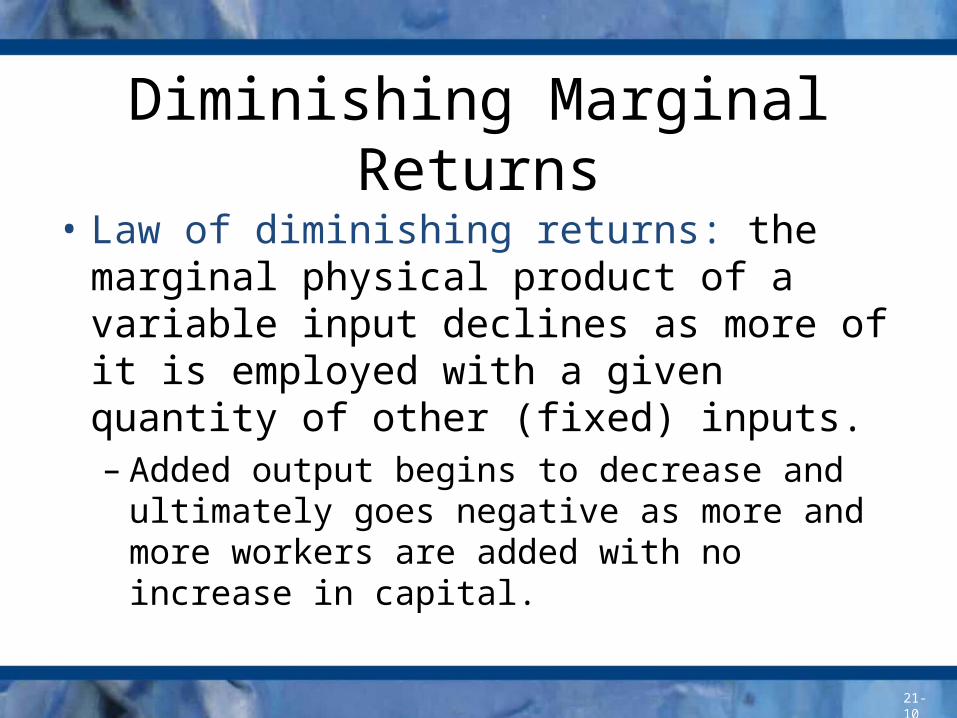
Diminishing Marginal Returns

• Law of diminishing returns: the marginal physical product of a variable input declines as more of it is employed with a given quantity of other (fixed) inputs.– Added output begins to decrease and ultimately

goes negative as more and more workers are added with no increase in capital.

21-11

Resource Costs

• The sales manager wants to maximize sales revenue.

• The production manager wants to minimize production costs.

• The business owner wants, instead, to maximize profit.

• There is no reason to expect these three goals to occur at the same output.

21-12

Resource Costs

21-13

Resource Costs

• As MPP decreases with added workers, we continue to pay the added workers, but we get less added product with each added worker.

• Therefore, the cost per added product increases as MPP declines.

• Marginal cost (MC): the increase in total cost associated with a one-unit increase in production.

21-14

Marginal Cost (MC)

• When MPP decreases, MC must increase, and vice versa.

• For any production with fixed capital, the MC curve will fall at low levels of production but will rise sharply at higher levels when diminishing marginal returns set in.

Change in total costMarginal cost (MC) = Change in output

21-15

Dollar Costs

• Total cost (TC): the market value of all resources used to produce a good or service.

• Fixed cost (FC): costs of production that don’t change when the rate of output is altered.

• Variable cost (VC): costs of production that change when the rate of output is altered.

Total Costs = Fixed costs + Variable costs TC = FC + VC

21-16

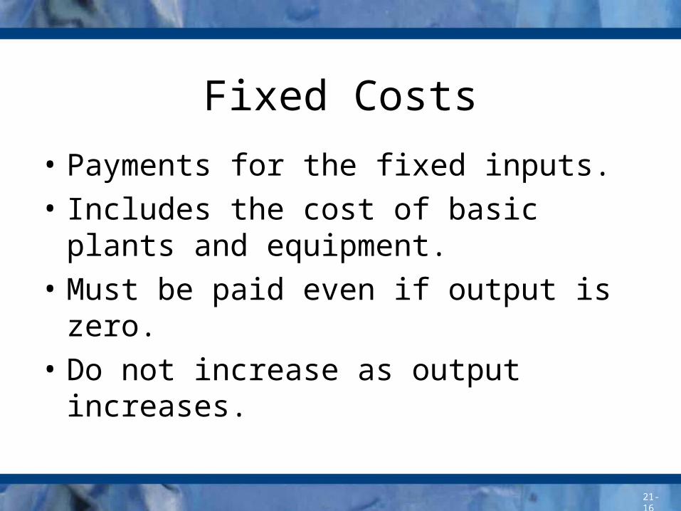
Fixed Costs

• Payments for the fixed inputs.• Includes the cost of basic plants and

equipment.• Must be paid even if output is zero.• Do not increase as output increases.

21-17

Variable Costs

• Payments for the variable inputs.• Include the costs of labor and raw materials.• At zero output, these costs are zero.• As output increases, variable costs increase

rapidly at first, then more slowly, and finally very fast as the firm approaches maximum capacity.

21-18

Average Costs• Average total cost (ATC): total cost divided by the

quantity of output in a given time period.– ATC = TC / q

• Average fixed costs (AFC): total fixed cost divided by the quantity of output in a given time period.– AFC = FC / q

• Average variable cost (AVC): total variable cost divided by the quantity of output in a given time period.– AVC = VC / q

21-19

Characteristics of the Cost Curves• Falling AFC: as output increases, AFC decreases

rapidly. Any increase in output will lower AFC.• U-shaped AVC: AVC decreases at first, hits a

minimum, and then rises as output increases (as a result of diminishing returns).

• U-shaped ATC: at low output, falling AFC dominates and ATC decreases. As output increases, rising AVC begins to dominate. ATC hits a minimum, then begins to rise.

21-20

Minimum Average Cost• The output at which ATC switches from being

dominated by AFC to being dominated by rising AVC is the point where average costs are minimal.– It is at this output where the firm can produce at

the lowest cost per unit...– … and where the firm minimizes the amount of

resources being used.– However, this amount of output is not necessarily

the output where profit is maximized.

21-21

Marginal Cost (MC)

• Diminishing returns in production cause MC to increase as output increases.

• After a brief drop in MC at low output, MC rises rapidly as output increases.

• As MC rises, it intersects ATC at its minimum point.

• ATC decreases when MC<ATC.• ATC increases when MC>ATC.

Change in total costMarginal cost (MC) = Change in output

21-22

Economic vs. Accounting Costs

• Accountants count only dollar costs of production – that is, the explicit costs. – Explicit costs: a payment made for the use of a

resource.

• Economists add the value of all other resources used in production, including resources not paid for in dollars. – Implicit costs: the value of resources used in

production, even when no direct payment is made.

21-23

Economic vs. Accounting Costs

• Explicit costs can be identified by the accountant with a paper trail denominated in dollars.

• Implicit costs are the cost of resources for which no payment is made – that is, the opportunity cost of using those resources. They can be identified only by the entrepreneur.

Economic cost = Explicit costs + Implicit costs

21-24

Long-Run Costs• The short run is characterized by fixed costs. – In the short run, the plants and equipment are

fixed.– The objective is to make the best use of those fixed

inputs while making the production decision.• In the long run, we can change the plants and

equipment.– Long run: a period of time long enough for all

inputs to be varied.– There are no fixed costs in the long run. All costs

are variable.

21-25

Long-Run Average Costs• In the long run, a firm

can build a plant of any desired size.

• As plant size gets larger, each plant’s ATC curve has a lower minimum point.

• In this case, building a larger plant would lower production costs.

21-26

Long-Run Average Costs• There are unlimited

options.• One option delivers

the lowest ATC. • It is at this point

where the long-run marginal cost curve intersects the long-run average total cost curve.

21-27

Economies of Scale

• Economies of scale: reductions in minimum average costs that come through increases in the size (scale) of plants and equipment.– Larger plants reduce minimum average costs.– Greater efficiency may come from• Specialization vs. multifunction workers.• Mass production vs. small batch mode production.

21-28

Diseconomies of Scale

• If the plant size gets too big, however, long-run average costs begin to rise, creating diseconomies of scale.– Operating efficiency may be reduced.– Worker alienation may increase.– Rigid corporate structures emerge.– Off-site management may be unresponsive.

• Bigger isn’t always better.