Chapter 2 Meshless Method

4

Chapter 2

Element Free Galerkin (EFG) method

2.1 Introduction

The element free Galerkin (EFG) method is a meshless method developed by Belytschko,

Lu and Gu (1994). This method only requires a set of nodes and a description of the

boundaries to construct an approximation solution. The connectivity between the data points

and the shape functions are constructed by the method without recourse to elements.

The EFG method employs the moving least square (MLS) approximations, which are

composed of three components: a weight function of compact support associated with each

node, a polynomial basis and a set of coefficients that depend on position. The support of the

weight function defines a node the domain of influence, which is the sub-domain over which

a particular node contributes to the approximation. The overlap of the nodal influence domain

defines the nodal connectivity.

One useful property of MLS approximations is that their continuity is equal to the

continuity of the weight function; highly continuous approximations can be generated by an

appropriate choice of the weight function. Although the EFG can be considered meshless with

respect to shape function construction or function approximation, a mesh will be required for

solving partial differential equations by the Galerkin approximation procedure. This is

because evaluation of the integrals in the weak form requires a subdivision of the domain

unless nodal quadrature is used.

CHAPTER 2: ELEMENT FREE GALERKIN METHOD 5

This chapter describes the construction of MLS approximations and the resulting EFG

shape functions in two types of support domains either circle or rectangle. In my work, the

second-derivatives of the shape function are required for equilibrium model in Chapter 3. So,

there are two cases to compute the second-order derivatives of the shape functions also

presented here. The first case is referred in the PhD thesis of Duflot (2004), Duflot (2005) and

Duflot and Nguyen-Dang (2001), (2004). And the other is in Belytschko, Lu and Gu (1994),

Dolbow and Belytschko (1998) and Liu (2003). In the course of this description, the effect of

different weight functions is illustrated.

Finally, the choice of the basic functions, the support and influence domain concepts are

defined on that. The determination of the dimension of a support domain and the detail

algorithm to compute the shape function and their derivatives are also presents in this chapter

as follows.

2.2 Moving least square (MLS) approximation

In this section, I would like to present the MLS approximation, which was introduced by

Lancaster and Salkauskas (1981) for smoothing and interpolating data. Currently the MLS

method is a widely used alternative for constructing meshless shape functions for

approximation. The first, Nayroles et al (1992) were used MLS approximation to construct

shape functions for their diffuse element method (DEM), after Belytschko, Lu and Gu (1994),

who named it the EFG method, where the MLS approximation is also employed.

This method employs MLS approximants to approximate the function with as

in Liu (2003), Fries and Matthies (2004), and Belytschko, Lu and Gu (1994). We consider a

sub-domain , the neighbourhood of a point

)(xu )(xu h

xΩ x and denoted as the domain of definition of

the MLS approximation for the trial function x , which is located in the problem domain Ω .

Let be the function of the field variable defined in the domain )(xu xΩ . The approximation of

at point )(xu x is denoted . The MLS approximation first writes the field function in

the form

)(xu h

(2.1) ∑ Τ==m

iii

h apu )()()()()( xaxpxxx

where is the number of terms of monomials, is a vector of basis functions that

consists most often of monomials of the lowest orders to ensure minimum completeness.

m )(xp


The coefficient are also functions of )(xia x , in the equation (2.1) is obtained at

any point

)(xia

x by performing a weighted least square fit for the local approximation, which is

obtained by minimizing the difference between the local approximation and the function. The

discrete norm as follows: 2L

∑=

−−=n

II

hI xuuxxwJ

1

2))()()(( x

(2.2) 2

1])()([)( II

n

II uxxxw −−= Τ

=∑ xap

where is a weight function with compact support and n is the number of points in

the neighbourhood of

)( Ixxw −

x , for which the weight function xΩ 0)( ≠− Ixxw , and is the

nodal value of at .

Iu

u Ixx =

iu

ix

)( ih xu

)(xu hu

x 0

• ••

••

•

Figure 2.1: The approximation function and the nodal parameters in the MLS approximation )(xu hiu

Equation (2.2) can be rewritten in the form

(2.3) ))(()( uPaxWuPa −−= ΤJ

there

(2.4) ),,,( 21 nuuu K=Τu

(2.5)

⎥⎥⎥⎥

⎦

⎤

⎢⎢⎢⎢

⎣

⎡

=

)()()(

)()()()()()(

21

22221

11211

nmnn

m

m

xpxpxp

xpxpxpxpxpxp

L

MOMM

L

L

P


and

(2.6)

⎥⎥⎥⎥

⎦

⎤

⎢⎢⎢⎢

⎣

⎡

−

−−

=

)(00

0)(000)(

)( 2

1

nxxw

xxwxxw

L

MOM

L

L

xW

The functional can be minimized by setting the derivative of with respect to equal

to zero i.e.,

J J a

0=∂∂

aJ . The following system of equation results: m

0])()()[(2)(0

0])()()[(2)(0

0])()()[(2)(0

1

12

2

11

1

∑

∑

∑

=

Τ

=

Τ

=

Τ

=−−⇔=∂∂

=−−⇔=∂∂

=−−⇔=∂∂

n

IIIImI

m

n

IIIII

n

IIIII

uxxxpxxwaJ

uxxxpxxwaJ

uxxxpxxwaJ

ap

ap

ap

MMM

(2.7)

This is in vector notation

∑ (2.8) =

Τ =−−n

IIIII uxxxxxw

10])()()[(2)( app

(2.9) 0)()()()()()(21

=−−−∑=

ΤIIII

n

III uxxxwxxxxxw papp

Eliminating the constant factor and separating the right hand side given

(2.10) ∑∑==

Τ −=−n

IIIII

n

III uxxxwxxxxxw

11)()()()()()( papp

or

(2.11) PuxWxaPPxW )()()( =Τ

So, we have

(2.12) uxBxAxa )()()( 1−=

with (2.13a) ∑=

ΤΤ −==n

IIII xxxxw

1)()()()()( ppPPxWxA

is often called moment matrix, and

])()()()()()([)()( 2211 nn xxxwxxxwxxxw pppPxWxB −−−== L (2.13b)


Finally, we substitute the equations (2.12), (2.13a) and (2.13b) into (2.1) and obtaining an

approximation of the form

(2.14) uxBxApx )()()()( 1−Τ= xu h

or more detail

(2.15) I

n

III

n

IIII

h uxxxwxxxxwxu ∑∑=

−

=

ΤΤ −⎥⎦

⎤⎢⎣

⎡−=

1

1

1)()()()()()()( ppppx

This can be written shortly as

(2.16) uxxx )()()(1

Τ

=

Φ== ∑n

III

h uu φ

where the shape function is defined by )(xΦ

(2.17) )()]()[()( 1 xBxAxpx −ΤΤ =Φ

and thus for one certain shape function Iφ at a point x

(2.18) )()()]()[()( 1III xxxw pxAxpx −= −Τφ

or (2.19) )()()()( xpxcx III wxΤ=φ

with (2.20) )()()( 1 xpxAxc −=

To compute the shape functions from (2.17) it is necessary to invert the A matrix. In one

dimension, this operation is not computationally expensive, but here we need to compute in

two or three dimensions it becomes burdensome. In this section, we present two cases to

compute the shape functions and their derivatives as following.

Case one: According to the PhD thesis of Duflot (2004), Duflot (2005), and Duflot

and Nguyen-Dang (2001), (2004). We have the first-order derivatives of the MLS shape

functions

(2.21) )()()()()()()( ,,, xpxcxpxcx kIIIIkkI wxwx ΤΤ +=φ

with

)()()()()()( ,1

,1

, xpxAxpxAxc kkk−− +=

)()()()()()( ,11

,1 xpxAxpxAxAxA kk

−−− +−=


)]()()()[( ,,1 xpxcxAxA kk +−= −

(2.22) ])[(1kbxA −=

and

(2.23) ∑=

Τ=n

IIIkIk xxw

1,, )()()()( ppxxA

The second-order derivatives are

++= ΤΤ )()()()()()()( ,,,, xpcxpxcx lIIkIIklklI wxxwxφ

(2.24) )()()()()()( ,,, xpxcxpxc klIIkIIl wxwx ΤΤ ++

with

)]()()()()()()()[()( ,,,,,,1

, xcxAxcxAxcxAxpxAxc klkllkklkl −−−= −

(2.25) ])[(1klbxA −=

and

(2.26) ∑=

Τ=n

IIIklIkl xxw

1,, )()()()( ppxxA

Case two: According to Belytschko, Lu and Gu (1994), Dolbow and Belytschko

(1998) and Liu (2003). This method involves the LU decomposition of the A matrix. The

shape function in (2.17) can be written as

(2.27) )()()()]()[()( 1 xBxxBxAxpx Τ−ΤΤ ==Φ γ

which leads to the relationship

)()()( xpxxA =γ (2.28)

the vector )(xγ can be determined using an LU decomposition of the A matrix and followed

by back substitution. The derivatives of )(xγ can be compute similarly, which leads to a

computationally efficient procedure for computing the derivatives of . We have )(xhu

γγ kkk ,,, ApA −= (2.29)


)( ,,,,,,, γγγγ klkllkklkl AAApA ++−= (2.30)

This leads to a simple relationship for the first derivatives of the shape function in (2.27)

given by

kkk ,,, BB γγ +=Φ (2.31)

and second-derivative is

klkllkklkl ,,,,,,, BBBB γγγγ +++=Φ (2.32)

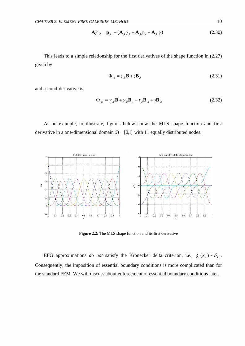
As an example, to illustrate, figures below show the MLS shape function and first

derivative in a one-dimensional domain ]1,0[=Ω with 11 equally distributed nodes.

Figure 2.2: The MLS shape function and its first derivative

EFG approximations do not satisfy the Kronecker delta criterion, i.e., IJJI x δφ ≠)( .

Consequently, the imposition of essential boundary conditions is more complicated than for

the standard FEM. We will discuss about enforcement of essential boundary conditions later.


2.3 . The basic functions In meshless methods, the shape functions depended on the basis functions, which play an

important role with respect to the accuracy of results in computational. So, in this thesis, we

approached the problems by both displacement and equilibrium models. Therein equilibrium

model needs the second-order derivatives of shape functions, so we need to choose the basis

function and also need the second order. Here, we discuss the use of the pure basic

polynomial in 1D and 2D according to the PhD thesis of Duflot (2004), Duflot (2005) as

follows.

1D 2D Constant ]1[ ]1[ Linear ],1[ x ],,1[ yx

Quadratic ],,1[ 2xx ],,,,,1[ 22 xyyxyx

Table 2.1: Basic polynomial in 1D and 2D

k,,AA and matrices and vector in the equation (2.1), (2.20) and (2.23) do not

depend on the evaluation point. So, if the size of the problem permits it, it is efficient to store

once for all these values at each node, together with the coordinates of the node and a pointer

to the weight function. Furthermore, we can benefit from the fact that the first basis function

is always the unit function and that the next basis functions are the coordinates if the basis is

at least linear. So, we can cleverly store only and find inside it the basis

and the coordinates . For example, for linear and quadratic functions, the dyadic products

of linear function are

kl,A )( Ixp

)()( II xx Τpp )( Ixp

Ix

(2.33) ⎟⎟⎟

⎠

⎞

⎜⎜⎜

⎝

⎛=Τ

2

2

1)()(

IIII

IIII

II

II

yyxyyxxx

yxxx pp

and quadratic function

(2.34)

⎟⎟⎟⎟⎟⎟⎟⎟

⎠

⎞

⎜⎜⎜⎜⎜⎜⎜⎜

⎝

⎛

=Τ

22

34

3224

2322

2232

221

)()(

II

III

IIIII

IIIIII

IIIIIIII

IIIIII

II

yxyxySYMyxyxxyxyyxyyxyxxyxxyxyxyx

xx pp


2.4 Concept of the support domain

In the solid body of the structure, we use the sets of nodes scattered in the problem

domain and its boundary. The density of the nodes depends on the accuracy requirement of

the analysis and the resources available.

The nodal distribution is usually not uniform and a denser distribution of nodes is often

used in the area where the displacement gradient is larger. To interpolate the value at a point

within the problem domain, we used the concept of the support domain at that points, this

domain included the number of nodes in a “small local domain”. This small local domain is

often called the support domain. A support domain of a point x determines the number of

nodes to be used to support or approximate the function value at x . It can have different

shapes and its dimension and shape can be different for different points of interest x , as

shown in figure 2.3 below.

The shapes most often used are circular or rectangular. We always use the concept of

support domain to select the nodes for constructing shape functions. These choices relate to

determine the dimension of the support domain. We can see in Liu (2003), Fleming (1997)

and Krongauz (1996).

Figure 2.3: The rectangular and circle support domains


2.5 Concept of the influence domain

We should understand and distinguish clearly between support and influence domains in

meshless methods. According to Liu (2003), and the PhD thesis of Fleming (1997) the

influence domain is defined as a domain that a node exerts an influence upon. It goes with a

node, in contrast to the support domain, which goes with a point of interest x that can be, but

does not necessarily have to be, at the node.

Use of an influence domain is an alternative way to select nodes for interpolation, and it

works well for domains with highly non-regularly distributed nodes. The influence domain is

defined for each node in the problem domain, and it can be different from node to node

represent the area of influence of the node, as shown in figure 3.5 below. Node 1 has an

influence radius of , node 2 has and node 3 has , etc. 3r1r 2r

xQ *Ωο 1

r1 ο 3

r3

ο 2r2

Γt

uΓ

tΓ

Figure 2.4: Influence domain of nodes

The node will be involved in the shape function construction for any point that is within

its influence domain. As above figure, in constructing the shape functions for the point ,

nodes 1 and 2 will be used, but node 3 will not be used. The fact that the dimension of the

influence domain can be different from node to node allows some nodes to have further

influence than others and prevents unbalanced nodal distribution for constructing shape

functions. Also in above figure, nodes 1, 2 are included for constructing shape functions for

the point , but node 3 is not included, even though node 3 is closer to compared with

node 1.

Qx

Qx Qx


2.6 Determination of the dimension of a support domain

In meshless methods, currently there are many methods to determine the dimension of a

support domain in problems depending on each of type difference problems. In fact, none

of methods can be totally suitable to all types of nodal distributions. In this thesis, we present

some relative methods to determine the dimension of a support domain.

dm

The accuracy of interpolation depends on the nodes in the support domain of the point of

interest, which is often a quadrature point or the center of integration cells. Therefore, a

suitable support domain should be chosen to ensure a proper area of coverage for

interpolation.

cs ddm α= (2.35)

with is a characteristic length that relates to the nodal spacing near the point of interest. If

the nodes are uniformly distributed, is simply the distance between two neighbouring

nodes. In the opposite case non-uniformly distributed, can be defined as a value average

nodal spacing in the support domain by computational the minimum, the maximum nodal

spacing for a given node. And

cd

cd

cd

sα is a coefficient that according to computed experience,

generally, a 4.1=sα to lead to good results. We can see this problem clearly in Liu

(2003), Liu and Gu (2003).

0.4

Moreover, we can use the method fixed minimum number of supporting points in the

domain of interpolation. This method may be suitable to cases the domain of problem such as

crack, plasticity or complex problem domain and currently, this method is used almost.

In my opinion, there are some remarks for this determination: we note that the accuracy

of interpolation depends on the nodes in the support domain of the point of interest. The first

it ensures that there are enough particles inside the support. The second, it makes sure that

there should not have too many particles inside a support. Because, if there are not enough

particles inside the support, when we calculate meshless shape function, we will encounter

singularity problem. If it has too many particles in a support, the bandwidth of stiffness matrix

will be large, so computationally it is not efficient. The third, with respect to above average

computation, we should take care the difference between the minimum and maximum support

size is not too large.


2.7 The weight functions

The weight functions play an important role in meshless methods. The weight function

should be non-zero only over a small neighbourhood of , called the domain of influence of

node

IxthI . This domain of influence will be defined latter. The various weight functions that

greatly affect the accuracy of the numerical results need to satisfy the following conditions

− , inside a sub-domain 0)( >xwi , xΩ− , outside the sub-domain 0)( =xwi , xΩ− is a monotonically decreasing function )(xwi

To understand more clearly and detail about the above conditions we can be refer to Liu

G.R. (2003), Belytschko, Lu and Gu (1994) and Shuyao and De’an (2003).

According to the PhD thesis of Organ (1996), the choice of the weight function

affects the resulting approximate function . As the illustration, consider the

three cases be shown in figure 2.5, figure 2.6 and figure 2.7 where the function is

approximated by using the nodal values at eleven spaced nodes, and using together a

linear polynomial basis . In each case, a representative weight function

corresponding to node 6 is plotted along with the resulting MLS approximation for the entire

domain.

)(xu h)( Ixxw −

)(xu

)(xu h

],1[ x=Τp

If we use the weight function unsuitable, it won’t get well for approximate solution. As a

result, we can scan to the plots below. For example, we consider the domain scattered by 11

nodes. The constant and cubic spline weight functions and resulting MLS approximations,

together with FEM approximation also shows follows

In figure 2.5, we used the constant weight function and the solution of MLS

approximation is linear. So in this case, the result is not good because of error between exact

and approximate solution is too large. Let’s look at in figure 2.6, when we used the cubic

spline weight function, it had given a better result. Together the FEM approximation is given

good result as figure 2.7.


Figure 2.5: Constant weight function and corresponding approximation result

Figure 2.6: Cubic spline weight function and corresponding approximation result


Figure 2.7: FEM approximation result

For more details, the size of support of weight function associated with node

should be chosen such that should be large enough to have a sufficiently large number of

nodes to cover the domain of definition of the MLS approximation for the trial function at

every sample point to ensure the regularity of A. A very small may result in a relatively

large numerical error in using Gauss numerical quadrature to calculate the elements in the

system matrix.

iiwIdm

Idm

Idm

On the other hand, should be also small enough to maintain the local character for

the MLS approximation. As above mentioned, we can see that the weight function affects the

resulting approximation, if the weight function is continuous then the shape functions are also

continuous.

Idm

In this thesis, we used the weight functions according to the thesis PhD of Dufot (2004),

Duflot (2005), Duflot and Nguyen-Dang (2001), (2004), Dolbow and Belytschko (1998) and

Liu (2003) as follows

a. Cubic spline weight function

⎪⎩

⎪⎨

⎧

>≤<−+−

≤+−=

1|s|if01||if44

||if44)( 2

13342

34

2132

32

1 sssssss

sw (2.36)


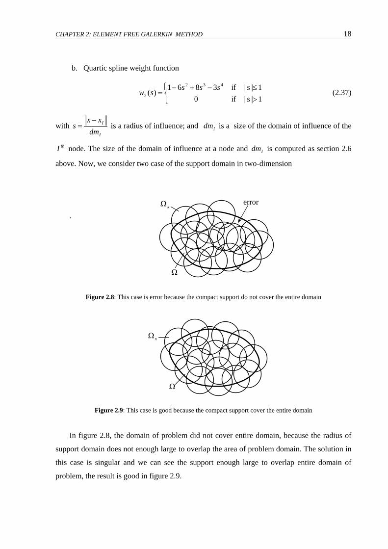
b. Quartic spline weight function

(2.37) ⎩⎨⎧

>≤−+−

=1|s|if01|s|if3861

)(432

2sss

sw

I

I

dmxx

s−

= is a radius of influence; and is a size of the domain of influence of the Idmwith

thI node. The size of the domain of influence at a node and is computed as section 2.6

above. Now, we consider two case of the support domain in two-dimension

Idm

error

Ω

xΩ.

Figure 2.8: This case is error because the compact support do not cover the entire domain

xΩ

Ω

Figure 2.9: This case is good because the compact support cover the entire domain

In figure 2.8, the domain of problem did not cover entire domain, because the radius of

support domain does not enough large to overlap the area of problem domain. The solution in

this case is singular and we can see the support enough large to overlap entire domain of

problem, the result is good in figure 2.9.


Figure 2.10: Cubic spline weight functions and first derivative in one-dimension

In two-dimension, the weight function corresponding to circle domain

⎟⎟⎠

⎞⎜⎜⎝

⎛ −=

i

iai dm

xxww )(x (2.39)

and rectangular domain

⎟⎟⎠

⎞⎜⎜⎝

⎛ −⎟⎟⎠

⎞⎜⎜⎝

⎛ −= y

i

iax

i

iai dm

yywdm

xxww ||||)(x (2.40)

Referring to the equations of derivative of the shape functions, it can be seen that the

spatial derivative of the weight function is necessary to compute the spatial derivative of the

A and B matrices. For circle domains in two-dimension is i

idm

xxs −= , for example with the

quartic spline weight function )(2 sw

2,2, )(i

ikkkki sdm

xxww −=x (2.41)


2,242,2

,2,))((

)(i

klk

i

illikkkklkli sdm

wdms

xxxxs

www

δ+

−−⎟⎟⎠

⎞⎜⎜⎝

⎛−=x (2.42)

with

(2.43) ⎩⎨⎧

>≤−+−

=1|s|if01|s|if122412

)(32

,2sss

sw k

(2.44) ⎩⎨⎧

>≤−+−

=1|s|if01|s|if364812

)(2

,2ss

sw kl

i

klikli dm

xw δ12)(,−

=if we have ; ixx = 1)( =ixw 0)(, =iki xw and

Similarly, for rectangular domain we used the tensor product weights follows

yxyxi wwswswxxw .)().()( ==− (2.45)

where and is given by (2.36) and (2.37) with replaced by and

respectively

)( xsw )( ysw xs yss

x

ix dm

xxs

−= (2.46)

y

iy dm

yys

−= (2.47)

xIx cdm α= yIy cdm α=with ; (2.48)

Thus derivatives of the weight function in (2.45) is calculated by

yx

x wdx

dww ., = (2.49)

xy

y wdy

dww ., = (2.50)

yx

xx wdx

wdw .2

2

, = (2.51)

xy

yy wdy

wdw .2

2

, = (2.52)


dydw

dxdww yx

xy ., = (2.53)

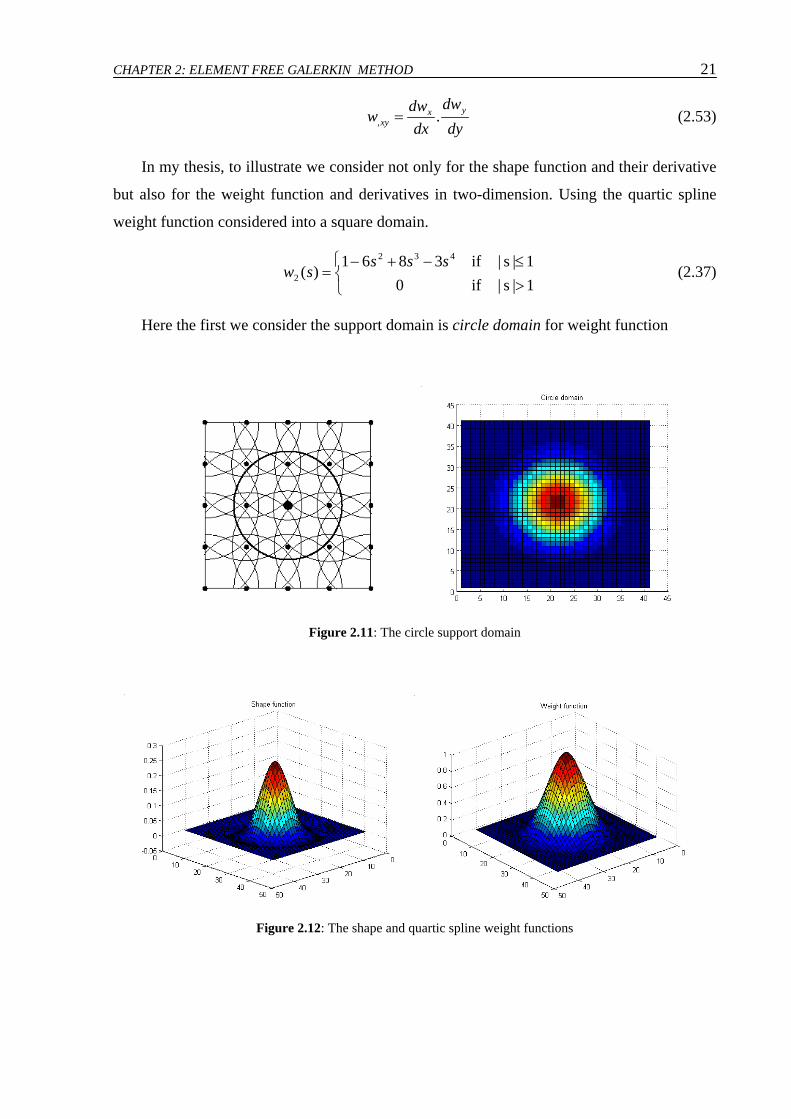
In my thesis, to illustrate we consider not only for the shape function and their derivative

but also for the weight function and derivatives in two-dimension. Using the quartic spline

weight function considered into a square domain.

(2.37) ⎩⎨⎧

>≤−+−

=1|s|if01|s|if3861

)(432

2sss

sw

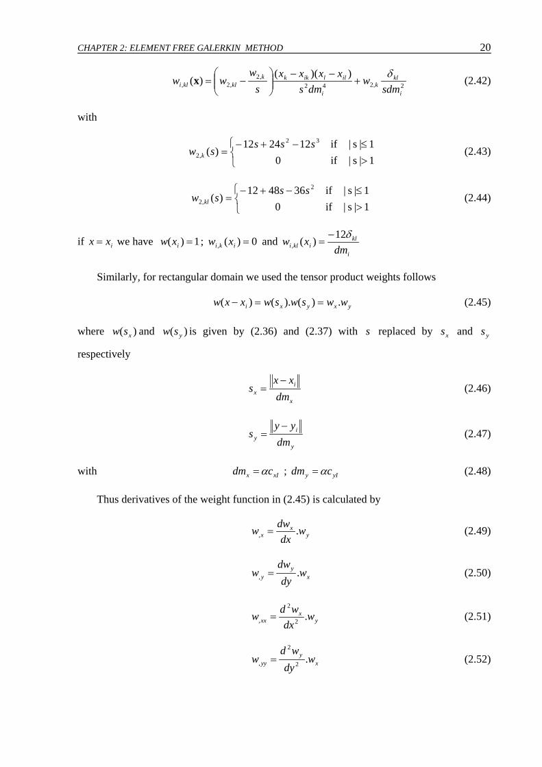
Here the first we consider the support domain is circle domain for weight function

Figure 2.11: The circle support domain

Figure 2.12: The shape and quartic spline weight functions


Figure 2.13: The x- derivatives of shape and weight functions

Figure 2.14: The y- derivatives of shape and weight functions

Figure 2.15: The xx- derivatives of shape and weight functions


Figure 2.16: The yy- derivatives of shape and weight functions

Figure 2.17: The yy- derivatives of shape and weight functions

In the derivatives of the shape and weight functions, the first- and second-derivatives are

must be symmetric.


The second we consider the support domain is rectangular domain for weight function

Figure 2.18: The rectangular support domain

Figure 2.19: The x- and y- derivatives of shape functions

Figure 2.20: The xx- and yy- derivatives of shape functions


2.8 Algorithm to compute the shape function and their derivatives , kI ,φIφ and klI ,φ

List of candidate nodes

of problem domain

Set up initial symmetric matrices A , k,A , kl,A

and )()( II xx Τpp are equal zero for 2,1, =lk .

Loop on all the candidate nodes and compute the weight function )(xIw and their derivatives )(, xkIw and )(, xklIw . If the weight

function of the candidates is non-zero, it is an influencing node

Determine the influence domain at point Ix

Store the weight function )(xIw and its derivatives )(, xkIw and )(, xklIw .

Add the contribution of this candidate to A by equation (2.13a), k,A by equation (2.23) and

kl,A by equation (2.26) for 2,1, =lk with the help of the pre-computed dyadic product

)()( II xx Τpp by equations (2.33) or (2.34).

Compute the Cholesky factorisation of A . We can use the computationally more efficient Cholesky factorisation instead of

the LU factorisation since A is symmetric definite positive.

Compute p

Compute pAc 1−= also by equation (2.20) with the help of the factorisation of A .

1


1

Compute k,p , kl,p . For 2,1, =lk

Compute k,c and kl,c by equations (2.22) and (2.25) with the help of the factorisation of A . For 2,1, =lk

Loop on all the influencing nodes ),2,1( nI L= for 2,1, =lk

Compute )()( IxpxcΤ , )()(, Ik xpxcΤ and )()(, Ikl xpxcΤ with the help of the pre-computed )( Ixp

Compute the shape function )(xIφ by equation (2.19) knowing )()( IxpxcΤ and the stored )(xIw

Compute kI ,φ and klI ,φ by equations (2.21) and (2.24)

knowing )()(, Ik xpxcΤ ; )()(, Ikl xpxcΤ ; k,c and kl,c , the pre-computed )( Ixp and the stored )(xIw , )(, xkIw and )(, xklIw .

End

Figure 2.21: Flowchart of algorithm to compute the shape function and their derivatives

This algorithm based on the PhD thesis of Duflot (2004) and Duflot (2005). Currently

there are many other methods to compute the MLS shape functions and their derivatives.


2.9 Weak form or variational formulation

The weak forms to be used in meshless methods are the same as those used in FEM. In

FEM, one seldom uses the constrained principles and weak forms. The procedures used in

applying these weak forms in meshless methods will be slightly different from those in FEM,

because of the difference in the forms of the shape functions. The integration domain may no

longer be the union of the element, and it may overlap depending on the meshless method

used.

The EFG method employed the Galerkin weak form to derive the discretize system

equations from strong form system equations. We will present in detail the Galerkin

variational principle or weak form of equilibrium equations are posed in the chapter three for

both models. Besides we will use the Lagrange multipliers to impose the essential boundary

conditions.

2.10 Conclusions

In the EFG method, the shape function does not satisfy the Kronecker delta criterion, i.e.,

IJJI x δφ ≠)( . Consequently, the imposition of essential boundary conditions is more

complicated than for the standard EFM. Currently, there are several methods have been

developed, including Lagrange multipliers Belytschko, Lu and Gu (1994), modified

variational principles Lu, Belytschko, and Gu (1994), and in the FE-EFG coupled method as

in Belytschko, Organ and Krongauz (1995), etc. These issues can be avoided if the essential

boundaries are along finite element domains, where the essential boundary conditions can be

prescribed directly as nodal values.

Properly choosing the domain of influence or nodal support is an important aspect of

meshless methods. The size of the support should be sufficiently large so that the moment

matrix is regular and well conditioned. So, the spatial distribution of neighbors is fairly even.

On the other hand, choosing domains of influence that are too large leads to a great deal of

computational expense in forming the approximations as well as assembling the stiffness

matrix. Support sizes that are too large also detract from the local character of the

approximation, for problems involving sharp gradients; some loss of accuracy is typically

noted as the effect of the gradient is smeared.


66 ×Figure 2.22: The example for the integration of Gauss quadrature point


In Chapter 3, to compute the stiffness and flexibility matrices, force vectors, etc requires

integration over the domain Ω or a part Γ . Which in two-dimensions corresponds to an area

integration. Currently there are many techniques to compute the numerical integration such as

cell quadrature, element quadrature or the technique of nodal integration was proposed by

Beissel and Belytschko (1996), Dolbow (1998), Dolbow and Belytschko (1999), etc. But in

this thesis, element quadrature is used with Gauss quadrature points in each cell by numerical

integration, for example as in figure 2.22.

Documents

Chapter 2 Meshless Method