University of Mississippi University of Mississippi

eGrove eGrove

Electronic Theses and Dissertations Graduate School

2012

Accelerating the Performance of a Novel Meshless Method Based Accelerating the Performance of a Novel Meshless Method Based

on Collocation With Radial Basis Functions By Employing a on Collocation With Radial Basis Functions By Employing a

Graphical Processing Unit as a Parallel Coprocessor Graphical Processing Unit as a Parallel Coprocessor

Derek Owusu-Banson

Follow this and additional works at: https://egrove.olemiss.edu/etd

Part of the Electromagnetics and Photonics Commons

Recommended Citation Recommended Citation Owusu-Banson, Derek, "Accelerating the Performance of a Novel Meshless Method Based on Collocation With Radial Basis Functions By Employing a Graphical Processing Unit as a Parallel Coprocessor" (2012). Electronic Theses and Dissertations. 217. https://egrove.olemiss.edu/etd/217

This Thesis is brought to you for free and open access by the Graduate School at eGrove. It has been accepted for inclusion in Electronic Theses and Dissertations by an authorized administrator of eGrove. For more information, please contact egrove@olemiss.edu.

ACCELERATING THE PERFORMANCE OF A NOVEL MESHLESS METHOD BASED ON

COLLOCATION WITH RADIAL BASIS FUNCTIONS BY EMPLOYING A GRAPHICAL

PROCESSING UNIT AS A PARALLEL COPROCESSOR

A Thesis

presented in partial fulfillment of requirements

for the degree of Master of Science

in the Department of Electrical Engineering

The University of Mississippi

by

DEREK OWUSU-BANSON

December 2012

Copyright Derek Owusu-Banson 2012

ALL RIGHTS RESERVED

ii

ABSTRACT

In recent times, a variety of industries, applications and numerical methods including the

meshless method have enjoyed a great deal of success by utilizing the graphical processing unit

(GPU) as a parallel coprocessor. These benefits often include performance improvement over the

previous implementations. Furthermore, applications running on graphics processors enjoy

superior performance per dollar and performance per watt than implementations built exclusively

on traditional central processing technologies. The GPU was originally designed for graphics

acceleration but the modern GPU, known as the General Purpose Graphical Processing Unit

(GPGPU) can be used for scientific and engineering calculations. The GPGPU consists of

massively parallel array of integer and floating point processors. There are typically hundreds of

processors per graphics card with dedicated high-speed memory.

This work describes an application written by the author, titled GaussianRBF to show the

implementation and results of a novel meshless method that in-cooperates the collocation of the

Gaussian radial basis function by utilizing the GPU as a parallel co-processor. Key phases of the

proposed meshless method have been executed on the GPU using the NVIDIA CUDA software

development kit. Especially, the matrix fill and solution phases have been carried out on the

GPU, along with some post processing. This approach resulted in a decreased processing time

compared to similar algorithm implemented on the CPU while maintaining the same accuracy.

Along the way, some challenges were faced. They are also discussed in the following chapters.

iii

DEDICATION

This thesis is dedicated to my family, who supported me each step of the way.

iv

LIST OF SYMBOLS

In this text all acronyms are defined as they are introduced. Italicized text refers to physical/mathematical quantities, programming code, or emphasized terminology. Additional attributed are applied to physical and mathematical variables, as defined below.

Matrices are represented by bold-italic attributes with an over-bar, as in𝑴 .

Vectors: Structural vectors (column arrays) are indicated by bold-italic text.

Scalar variables are represented using italicized text.

When discussing equations the shorthand notation LHS and RHS are used to refer to the expressions to the left and right hand side of the equal sign respectively.

v

ACKNOWLEDGEMENTS

I would like to thank Dr Elliott Hutchcraft and Dr Richard Gordon for their guidance and

wisdom, and all my friends for their help and motivation over the years.

vi

TABLE OF CONTENTS ABSTRACT ............................................................................................................................................... ii

DEDICATION ........................................................................................................................................... iii

LIST OF SYMBOLS.................................................................................................................................... iv

ACKNOWLEDGEMENTS ............................................................................................................................ v

LIST OF FIGURES ....................................................................................................................................viii

INTRODUCTION ....................................................................................................................................... 1

1. GENERAL PUROPOSE GRAPHICAL PROCESSING UNITS ...................................................................... 3

GPU COMPUTING ................................................................................................................................ 4

GRAPHICS PIPELINE ............................................................................................................................. 7

GRAPHICS APIs .................................................................................................................................... 9

PROGRAMMABLE GRAPHICS HARDWARE .......................................................................................... 10

SYSTEM ARCHITECTURE ..................................................................................................................... 13

GPU FLOATING-POINT PERFORMANCE .............................................................................................. 15

GPGPU FOR SOLVING PARTIAL DIFFERENTIAL EQUATIONS ................................................................. 16

2. OVERVIEW OF CUDA TECHNOLOGY ............................................................................................... 18

THE GEFORCE 8 ARCHITECTURE ......................................................................................................... 19

CUDA C PROGRAMMING MODEL ....................................................................................................... 24

DEDICATED HIGH PERFORMANCE COMPUTING ................................................................................. 27

CUBLAS and CUFFT ............................................................................................................................ 28

3. MATHEMATICAL BACKGROUND ..................................................................................................... 29

OVERVIEW OF MESHLESS IN ELECTROMAGNETICS ............................................................................. 31

RADIAL BASIS FUNCTION ................................................................................................................... 33

NOVEL MESHLESS METHOD ............................................................................................................... 35

4. CUDA IMPLEMENTATION ............................................................................................................... 41

C REFERENCE PROGRAM.................................................................................................................... 41

CODE PARALLLELIZATION................................................................................................................... 42

THE GAUSSIANRBF CUDA KERNELS .................................................................................................... 43

vii

PERFORMANCE .................................................................................................................................. 49

LIMITATIONS ..................................................................................................................................... 76

5. CONCLUSION ................................................................................................................................. 77

6. REFERENCES .................................................................................................................................. 79

7. APPENDICES .................................................................................................................................. 85

8. VITA ............................................................................................................................................... 91

viii

LIST OF FIGURES

Figure 1.1. GPU Devotes More Transistors to Data Processing ...................................................6 Figure 1.2. Conceptual Illustration of Graphics Pipeline ..............................................................8 Figure 1.3. Instruction based processing .................................................................................... 11 Figure 1.4. Data stream processing ............................................................................................ 12 Figure 1.5. The overall system architecture of a typical PC ....................................................... 14 Figure 1.6. Floating-point performance of commodity Intel CPUs versus commodity ATI and

NVIDIA GPUs................................................................................................................... 16 Figure 2.1. NVIDIA GeForce 8800 GTX block diagram. Image courtesy Owens et al[11] ........ 20 Figure 3.1. Processes that lead to building a complicated engineering system [16] .................... 30 Figure 3.2. Problem domain ...................................................................................................... 36 Figure 3.3. Enforcing equations 5 and 6 at different points on the problem domain ................... 39 Figure 4.1. Different block shapes ............................................................................................. 43 Figure 4.2. Shared memory ....................................................................................................... 44 Figure 4.3. Description of GaussianRBF kernel algorithm ......................................................... 45 Figure 4.4. Dense Matrix Fill Code ........................................................................................... 47 Figure 4.5 A 2D Hierarchy of Blocks and Threads used in the Dense Matrix Fill ..................... 48 Figure 4.6. Execution time for matrix fill using Intel i7 CPU and NVIDIA GeForce GTX 460

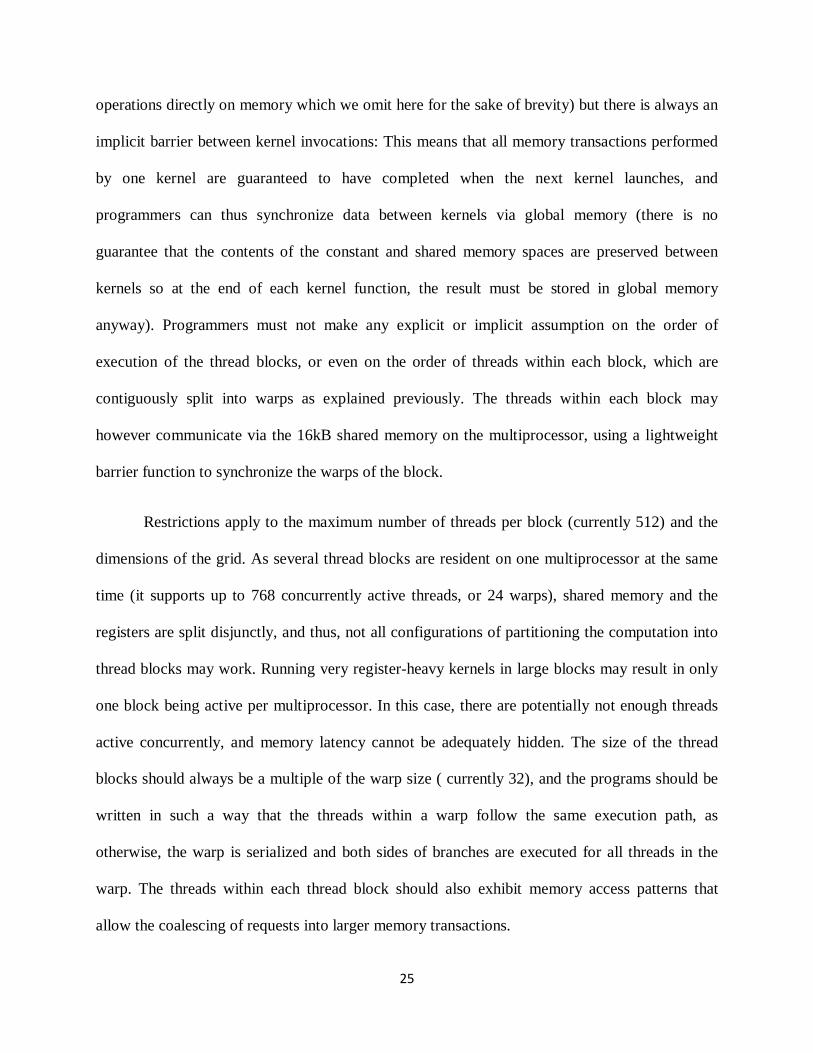
GPU. .................................................................................................................................. 51 Figure 4.7. Speedup for matrix fill using Intel i7 CPU and NVIDIA GeForce GTX 460 GPU ... 52 Figure 4.8. Execution time for summation using Intel i7 CPU and NVIDIA GeForce GTX 460

GPU. .................................................................................................................................. 53 Figure 4.9. Speedup for summation using Intel i7 CPU and NVIDIA GeForce GTX 460 GPU .. 54 Figure 4.10. Execution time for matrix solution using Intel i7 CPU and NVIDIA GeForce GTX

460 GPU. ........................................................................................................................... 55 Figure 4.11. Speedup for matrix solution using Intel i7 CPU and NVIDIA GeForce GTX 460

GPU ................................................................................................................................... 56 Figure 4.12. Overall Execution time using Intel i7 CPU and NVIDIA GeForce GTX 460 GPU . 57 58 Figure 4.13 Overall Speedup factor using Intel i7 CPU and NVIDIA GeForce GTX 460 GPU .. 58 Figure 4.14. Execution time for matrix fill using Intel i3 CPU and NVIDIA GeForce GT 525M

GPU. .................................................................................................................................. 59 Figure 4.15. Speedup curve for matrix fill using Intel i3 CPU and NVIDIA GeForce GT 525M

GPU. .................................................................................................................................. 60

ix

Figure 4.16. Execution time for summation of using Intel i3 CPU and NVIDIA GeForce GT 525M GPU. ........................................................................................................................ 61

Figure 4.17. Speedup for summation using Intel i3 CPU and NVIDIA GeForce GT 525M GPU. .......................................................................................................................................... 62

Figure 4.18. Execution time for matrix solution using Intel i3 CPU and NVIDIA GeForce GT 525M GPU. ........................................................................................................................ 63

Figure 4.19 Speedup factor for matrix solution using Intel i3 CPU and NVIDIA GeForce GT 525M GPU. ........................................................................................................................ 64

Figure 4.20 Overall Execution time using Intel i3 CPU and NVIDIA GeForce GT 525M GPU. 65 Figure 4.21 Processing Time for Matrix Fill .............................................................................. 66 Figure 4.22 Processing Time for Summation ............................................................................. 67 Figure 4.23. RMSE Analysis on the CPU and GPU ................................................................... 68 Figure 4.24. Pseudo code of the Jacobi Preconditioned BiCG Method ....................................... 70 Figure 4.25. Execution time for summation using BiCG solver ................................................. 71 Figure 4.26. Speedup for summation using BiCG solver........................................................... 72 Figure 4.27. Execution time for matrix solution using BiCG solver ........................................... 73 Figure 4.28. Speedup for matrix solution using BiCG solver ..................................................... 74 Figure 4.29 RMSE Analysis for CPU and GPU using the Iterative Solver ................................. 75

1

INTRODUCTION

The performance of Graphical Processing Units or GPU has been improved significantly

in recent years. Compared with the CPU, the GPU is better suited for parallel processing and

vector processing and has evolved to perform various types of computations. General-purpose

computations on GPUs (GPGPU) have been examined for various applications.

The purpose of this research is to develop a program that uses a novel proposed meshless

method based on collocation with radial basis functions and increase speed up by implementing

key phases on the graphical processing unit (GPU). In the past, the numerical solution of the

electromagnetic (EM) wave equation has commonly been obtained by using the finite element

methods (FEM) and finite difference methods (FDM). However, the lack for robust and efficient

3D mesh generators makes the solution of 3D problems a difficult task. Furthermore, mesh-

based methods are also not well suited to the problems associated with extremely large

deformation and problems associated with frequency remeshing. To avoid these drawbacks of

the FEM, considerable effort has been devoted during recent years to the development of

meshless methods. The novel proposed meshless method uses the Gaussian radial basis function

(RBF) to expand the potential.

In the development process, several software packages were tested for implementing

stages within the overall meshless method sequence on the GPU. Extensive experimentation was

carried out on both the GPU global matrix fill and the GPU matrix equation solution stages.

Numerous techniques will be presented along with their motivation and background, in an

2

attempt to provide a comprehensive examination into the process of developing solution to the

EM wave equation employing the graphics hardware.

3

1. GENERAL PUROPOSE GRAPHICAL PROCESSING UNITS

Graphics processing units (GPUs) are primarily designed for one particular class of

applications, rasterization and depth-buffering based interactive computer graphics. One could

argue that this is no longer the case as certain features are being added to the processors that are

not needed in graphics workloads, a consequence of GPUs transforming into a viable general-

purpose (data-parallel) computing resource known as GPGPU, general-purpose graphical

processing unit.

In the last decade, the performance of the Graphical Processing Units (GPU) has been

dramatically increased by the development of novel technology. In the beginning, a graphics

card was designed for purpose of display, so the main features of a graphics card were 2D

Graphics such as the number of colors, the quality of display, and the support of high resolution.

In the mid 1990s, enhanced Operating Systems (O/S) with user friendly Graphics User Interface

(GUI) led to demanding multi-media environments in order to play video files, to support 3D

graphics games, and to manage multiple displays. The demands of 3D graphics led to the

creation of the GPU, which had better integration and faster speed. In 2000, the multi-core

platform was incorporated in the design of GPU. Major vendors such as ATI, NVIDIA, and 3D

Labs competed to develop real time 3D graphics capable GPUs and they used the multi-core

technology for parallel processing. Now, floating point performance of the GPU is higher than

performance of the CPU because the architecture of the GPU is dramatically changed via

4

improvement of the chip design and manufacturing technology [1]. Thus people want to use this

great capability for general purpose applications.

GPU COMPUTING

At the present time, the GPUs are the most economical and powerful computational

hardware because they are inexpensive and user programmable, and they achieve high

performance. The increased flexibility and high computing capabilities of GPUs have led to a

new research field that explores the performance of GPUs for general purpose computation. The

general purpose computation on the GPU (GPGPU) is getting the attention of many researchers

and developers [2].

Graphics processing in the GPU is like an assembly line with each stage affecting

successive stages and all stages working in parallel. This architecture is called graphics pipeline.

The technology of the GPU has evolved into a more flexible programmable pipeline, and the

graphics pipeline has been replaced by the user programmable vertex shader and pixel shader.

“ A programmer can now implement custom transformation, lighting, or texturing algorithms by

writing programs called shaders”[3]. The pixel shader is more flexible than vertex shader to

program the GPGPU applications. Recent GPUs have fully programmable unified processing

units with support for single precision floating-point computation. Furthermore, the latest

generation of GPUs, such as ATI’s RV770 and NVIDIA’s GT200, is expanding on its

capabilities to support double precision floating point computation [4]-[5]. High speed, increased

precision, and rapidly expanding programmability of GPUs have transformed GPUs to a

powerful platform for general purpose computations.

5

Most modern PCs have programmable GPUs. Such GPUs typically give a floating point

computational power that is more than one order of magnitude higher compared to the CPU in

modern PC. In the coming decade, the computational power of GPUs is expected to grow

considerably faster than the computational power of CPUs, because the GPU architecture is more

scalable.

While CPUs are instructional driven, GPUs are data-stream driven. This means that the

GPU executes the same instruction sequence on large data sets. The instruction sequence to be

executed is uploaded to the GPU, before the execution is triggered by a data-stream being

assigned. The result of the computation can then be used for visualization, processed by a new

instruction sequence, or read back to the CPU. The use of parallel processing has traditionally

been hampered by the high cost of specialized hardware. With the current introduction of

clusters and more recently, multi-core CPUs, the cost of hardware for parallel processing is

drastically reduced.

The reason behind the discrepancy in floating-point capability between the CPU and the

GPU is that the GPU is specialized for compute-intensive, highly parallel computation and

therefore designed such that more transistors are devoted to data processing rather than data

caching and flow control, as shown in Figure 1.1 [6]

6

Figure 1.1. GPU Devotes More Transistors to Data Processing

More specifically, the GPU is especially well-suited to address problems that can be

expressed as data-parallel computations. Meaning the same program is executed on many data

elements in parallel with high arithmetic intensity. Because the same program is executed for

each data element, there is a lower requirement for sophisticated flow control, and because it is

executed on many data elements and has high arithmetic intensity, the memory access latency

can be hidden with calculations instead of big data caches.

Data-parallel processing maps data elements to parallel processing threads. Many

applications that process large data sets can use a data-parallel programming model to speed up

the computations. In 3D rendering, large sets of pixels and vertices are mapped to parallel

threads. Similarly, image and media processing applications such as post-processing of rendered

images, video encoding and decoding, image scaling, stereo vision, and pattern recognition can

map image blocks and pixels to parallel processing threads. In fact, many algorithms outside the

7

field of image rendering and processing are accelerated by data-parallel processing, from general

signal processing or physics simulation to computational finance or computational biology. [6]

GRAPHICS PIPELINE

All commodity GPUs and the APIs-application programming interfaces-used to program

them are organized in a so-called graphics pipeline. This concept was first introduced by Silicon

Graphics Inc. (SGI) in 1992 with the first version of the OpenGL standard, even though at that

time, not all features were implemented in hardware. As an abstraction of the actual

implementation, the pipeline divides the computation (i.e the rendering of an image into several

disjunct stages which are explained below. The pipeline is feed-forward, which naturally leads to

task parallelism between the stages. Within each stage, data parallelism is trivially abundant, as

all primitives are treated separately. From a hardware perspective, the pipeline concept removes

the necessity of expensive control logic to counteract typical hazards induced by the parallelism

such as read-after-write, write-after-read, and synchronization, deadlocks and other race

conditions. To maximize throughput over latency, the pipeline is very deep, with thousands of

primitives in flight at a time. In a CPU, any given operation may take on the order of 20 cycles

between entering and leaving the processing pipeline (assuming a level-1 cache hit for data); on

the GPU, in contrast, operations may take thousands of cycles to finish. In summary, the

implementation of the graphics pipeline in hardware allows to dedicate a much larger percentage

of the available transistors to actual computation rather than to control logic, at least compared to

commodity CPU designs.

8

CPUs are dealing with memory bandwidth and latency limitations by using ever-larger

hierarchies of caches. The working set sizes of graphics applications have grown approximately

as fast as transistor density. Therefore, it is prohibitive to implement a large enough caching

hierarchy on the GPU chip that delivers a reasonably high cache hit rate and maintains

coherency. GPUs do have caches, but they are comparatively small and optimized for spatial

locality, as this is the relevant case in texture filtering operations. More importantly, the memory

subsystem is designed to maximize streaming bandwidth ( and hence, throughput) by latency

tolerance, page-locality, minimization of read-write direction changes and even lossless

compression.[3]

Finally, another important aspect is that the market volume of interactive computer games

amounts to billions of dollars per year, creating enough critical mass and market pressure to

drive rapid hardware evolution, in terms of both absolute performance and broadening feature set

(economies of scale). Figure 1.2 depicts a simplified graphics pipeline.

Figure 1.2. Conceptual Illustration of Graphics Pipeline

9

GRAPHICS APIs

The hardware is not exposed directly to the programmer; in fact, most details of the

hardware realization of the graphics pipeline are proprietary and largely secret. Instead, well-

defined APIs offer a set of data containers and functions to map operations and data to the

hardware. These APIs are typically implemented by the vendors as a set of libraries and header

files interacting with the low-level device driver.

DirectX (more specifically, Direct3D as a subset of DirectX) and OpenGL are the two

dominant APIs to program graphics hardware. DirectX is restricted to Microsoft Windows ( and

Microsoft’s gaming consoles such as the Xbox), while Open GL has been implemented for, e.g.,

Windows, Linux, MacOS and Solaris. Both APIs are defined by consortia in which hardware and

software vendors collaborate closely. The DirectX specification is headed by Microsoft, whereas

the open Khronos group leads the development of OpenGL, more specifically, the OpenGL ARB

(architecture review board) as part of the Khronos consortium. The pipeline concept has been

integral component of both APIs since their initial revisions, in 1995 and 1992 respectively.

As both APIs map to the same hardware, there is usually a one-to-one correspondence;

typically, no (major) features exist that are only exposed through one of the APIs. The

fundamental design difference between the two APIs is how new hardware features are exposed.

The goal of DirectX is to specify a set of features that hardware must implement for a longer

product cycle, typically three years. It is therefore convenient to identify a certain class of GPUs

by the highest DirectX version it supports, one speaks for instance of DirectX 10 class hardware.

As the hardware development cycles are usually shorter, OpenGL includes the concept of

10

extensions to expose new or experimental features faster. Not all extensions are supported on all

hardware, and software developers have to check at runtime if a given extension is supported.

Only after extensions are supported by a wide range of GPUs, then they are considered for

inclusion in the OpenGL core and consequently, the OpenGL version numbers are incremented

at a slower rate than for DirectX.

In the domain of computer games, DirectX is almost exclusively used, and with Linux

increasing its market shares, is not even restricted to Microsoft Windows alone anymore.

However, in academia and for “professional” applications, OpenGL is often favored.

PROGRAMMABLE GRAPHICS HARDWARE

The reason why GPUs are well suited for general-purpose computations lies in the

architecture. GPUs are stream processors and are therefore designed to uniformly process large

amounts of data. As a consequence of this, the memory on a graphics card is fast and the internal

bandwidth is very high.

Data processing on a CPU is traditionally based on an instruction driven model as

illustrated in Figure 1.3. This model is called Single Instruction, Single Data (SISD) and

corresponds to the von Neumann architecture. In this architecture, a single processor executes a

single instruction stream to operate on data stored in the same memory as the instructions. The

instructions needed in the execution of the program in turn refer to data, or to other instructions

in the case of branching. The data needed for the execution of an instruction are loaded into the

cache memory during the processing.

11

Figure 1.3. Instruction based processing

The cache is a high-speed memory integrated on a chip (e.g., the CPU). If the data are not

present in cache, they are loaded from the system memory over the relatively slow front-side

bus. This makes instruction driven processing flexible but also inefficient when it comes to

uniform operations on large blocks of data.GPUs are based on data-stream processing using a

model called Single Instruction, Multiple Data (SIMD). In this model, the processor is first

configured by the instructions that will be executed, and then the data stream is processed as

illustrated in Figure 1.4. In other words, all data are processed by the same instructions until the

processor is reconfigured. This model often leads to cache-friendly implementations on the GPU.

The execution is parallelized by distributing the processing among several pipelines doing the

same operations.

12

Figure 1.4. Data stream processing

The computing paradigms for the CPU and the GPU are very different because the CPU

is traditionally based on an instruction driven model, while the GPU is based on a stream

processing model. As an example one may want to create a 𝑚 × 𝑛 matrix C by adding two

𝑚 × 𝑛 matrices A and B. On the CPU, the addition of the two matrices is done by a double for-

loop, where we transverse all elements in the matrix and do the computations sequentially, e.g.,

// instruction stream

for (i=0; i<m; i++)

for (j=0; j<n; j++)

C[i][j] = A[i][j] + B[i][j];

In the stream based computing model, we set up a data stream consisting of the two

matrices A and B as input and matrix C as output. Then we create a computational kernel that

takes one element from each data stream, adds them, and outputs the result. Finally the

corresponding processing pipeline is “executed”. In pseudo-code, this reads:

13

// data stream

setInputArrays (A, B);

setOutputArrays (C);

loadKernel (“matrix_sum_kernel”);

execute ();

where the computational kernel simply corresponds to:

return (A[i][j] + B[i][j]);

As opposed to traditional instruction-driven algorithms, the nested for-loop and the call to the

computational kernel never appear explicitly in the code. The for-loop is replaced by the

mechanism that feeds the two input streams through the processing pipeline, and the

computational kernel is called ‘automatically’ each time new elements from the two input

streams arrives at one of the data-processing units.

On the GPU, our abstract processing pipeline is the graphics pipeline that renders

graphics primitives to the screen. To add the matrices, we simply draw a rectangle with a

resolution of 𝑚 × 𝑛 pixels, and set the color of each pixel in the rectangle equal to the sum of

the corresponding pixels in the two 𝑚 × 𝑛 input textures A and B. The for-loop is then called

implicitly when the geometry is rendered.

SYSTEM ARCHITECTURE

The overall system architecture of a PC can be illustrated as in Figure 1.5. The North

Bridge and the South Bridge are the two main motherboard chips and together these are often

referred to as the chipset. The North Bridge typically handles the communication between CPU,

14

memory, graphics card, and the South Bridge. The South Bridge handles communication with

the “slower” peripherals, like the network card, the hard-disk controller, and more. In some

systems these controllers are included in the South Bridge. The front-side bus (FSB) is the term

used to describe the data bus that carries all information passing from the CPU to other devices

within the system.

Figure 1.5. The overall system architecture of a typical PC

In a computer system (as of 2006) the communication between the CPU and the GPU is

through a graphics connector called the PCI Express, which has a theoretical bandwidth of 4

GB/s simultaneously in each direction.

The internal memory bandwidth of the GPU is typically one order of magnitude higher

compared to the CPU memory interface. For instance, the CPU memory interface is 6.4 GB/s

15

with a 800 MHz FSB, whereas on a NVIDIA GeForce 7800 GTX 512 GPU, the bandwidth is 55

GB/s. Algorithms that run on the GPU can take advantage of this higher bandwidth to achieve

performance improvements, and this is one of the main reasons why GPUs are well suited for

general-purpose computations.

GPU FLOATING-POINT PERFORMANCE

Modern GPUs have high number of pipelines performing the same type of operations,

e.g., the new ATI chip with code name R600 is expected to have 64 pipelines. A higher number

of pipelines gives the GPU a higher degree of parallelism. The GPU is designed to process 4-

component floating-point vectors. Arithmetic operations that can be performed simultaneously

for all four components are therefore implemented efficiently in a GPU.

Implementations that take advantage of the GPU architecture can give very high floating-

point performance. Figure 1.6 is based on data from GPU-Bench [7], and illustrates the

performance of CPUs versus GPUs in recent years. The performance gap between CPUs and

GPUs is expected to grow, making GPUs even more attractive as a computational resource in the

future.

16

Figure 1.6. Floating-point performance of commodity Intel CPUs versus commodity ATI and NVIDIA GPUs

GPGPU FOR SOLVING PARTIAL DIFFERENTIAL EQUATIONS

As early as 2001, even in the earliest stages of GPGPU, methods were already being

developed to solve popular differential equations such as the Navier-Stokes fluid dynamics

equations [8] and the heat equation [9]. To facilitate this, these applications typically involved

replicating the input data as a texture- a technique still employed by models today. Also, these

techniques required ways to emulate common linear algebra functions.

More specifically to electromagnetics and partial differential equations, in 2005 Inman

and Elsherbeni [10] used the GU to perform finite difference time domain computations. In 2006

Baron et. al. [11] used the GPU to simulate the propagation of wireless signals within an indoor

environment. Woolsey et al [12] in 2007 increased the performance of a finite element method

electromagnetics simulation using GPU. Zainud-Deen et.al. [13] used AMD’s Brook+ GPGPU

17

model to solve Maxwell’s equations using a GPU based finite difference frequency-domain

method.

18

2. OVERVIEW OF CUDA TECHNOLOGY

In November 2006, NVIDIA unveiled the industry’s first DirectX 10 GPU, the GeForce

8800 GTX. The GeForce 8800 GTX was also the first GPU to be built with NVIDIA’s CUDA

Architecture. This architecture included several new components designed strictly for GPU

computing and aimed to alleviate many of the limitations that prevented previous graphics

processors from being legitimately useful for general-purpose computation. Unlike previous

generations that partitioned computing resources into vertex and pixel shader, the CUDA

Architecture included a unified shader pipeline, allowing each and every arithmetic logic unit

(ALU) on the chip to be marshaled by a program intending to perform general-purpose

computations [14]. These ALUs were built to comply with IEEE requirements for single-

precision floating-point arithmetic and were designed to use an instruction set tailored for

general computation rather than specifically for graphics. The execution units on the GPU were

allowed arbitrary read and write access to memory as well as to software-managed cache known

as shared memory. All of these features of the CUDA Architecture were added in order to create

a GPU that would excel at computation in addition to performing well at traditional graphics

tasks. At the time of launch, NVIDIA spelled out the acronym as Compute Unified Device

Architecture but has since transitioned to using it as a fixed term as explained earlier.

19

THE GEFORCE 8 ARCHITECTURE

The GeForce 8800 GTX (chip name G80) is the first CUDA-capable GPU at the time of

launch. The GeForce 8 also is the first GPU complaint with the DirectX 10 specification. Figure

2.1 shows a functional block diagram of the GeForce 8800 GTX (chip name G80).

The design is built around a scalable processor array (SPA) of stream processor “cores”

(ALUs also called thread processors, abbreviated SP), organized as streaming multiprocessors

(SM) or cooperative thread arrays (CTA) of eight SPs each, which in turn are grouped in pairs

into independent processing units called texture processor clusters (TPC) [15]. The GeForce

8800 GTX comprises 16 multiprocessors for a total of 128 thread processors. By varying the

number of SMs per chip, different price-performance regimes can be targeted.

20

Figure 2.1. NVIDIA GeForce 8800 GTX block diagram. Image courtesy Owens et al[16]

At the highest level, the SPA performs all computations, and shader programs from the

programmable stages are mapped to it using dynamic load balancing in hardware. The memory

system is also designed in a scalable way, with external, off-chip DRAM control and

composition processors (ROP – raster operation processors) performing color and depth frame

buffer operations like antialiasing and blending directly on memory streams to maximize

performance. A powerful interconnection network (realized via a crossbar switch) carries

21

computed pixel values from the SPA to the ROPs, and also routes (texture) memory requests to

the SPA, using on-chip level-2 caches. As in previous designs, these caches are optimized for

streaming throughput and strongly localized data reuse.

All fixed-function hardware is grouped around the SPA. The data flow for a typical

rendering task and thus, the mapping of the graphics pipeline to this processor, is as follows: The

input assembler collects per vertex operations and a dedicated unit distributes them to the

multiprocessors in the SPA, which executes vertex and geometry shader programs. Results are

written into on-chip buffers, and passed to the Setup-Raster-ZCull unit, in short the rasterizer,

which continues to be realized as fixed-function hardware for performance reasons. Rastered

fragments are routed through the SPA analogously, before being sent over the interconnection

network to the ROPs and to off-chip memory. The SPA accepts and processes work for multiple

logical streams simultaneously, to allow for dynamic load balancing. A dedicated unit called

computes work distribution dispatches blocks of work accordingly. Three different clock

domains control the chip, the reference design of G80-based graphics boards prescribes the

following values: Most fixed-function and scheduling hardware uses the core clock of 575 MHz,

the SPA runs at 1350 MHz, and the GDDR3 memory is clocked at an effective 1.8 GHz (900

MHz double data rate). The chip is fabricated in a 90nm process and comprises almost 700

million transistors, a significant increase compared to 220 million for the GeForce 6800 Ultra,

which is only two generations older.

The streaming multiprocessor is at the core a unified graphics and compute processor.

Each SM comprises eight streaming processor cores (ALUs), two special function units, a

multithreaded instruction fetch and issue unit, disjunct data and instruction level-1 caches, a

read-only constant cache and 16kB shared “scratchpad” memory allowing arbitrary read and

22

write operations. Each ALU comprises scalar floating point multiply-add as well as integer and

logic operations, whereas the special function units provide transcendental (trigonometric, square

root, logarithm and exponentiation) functions as well as four additional scalar multipliers used

for attribute interpolation.

To dynamically balance the shifting vertex, geometry, pixel and compute thread

workloads, each multiprocessor is hardware multithreaded, and able to manage and execute up to

768 concurrent threads with zero scheduling overhead. The total number of threads concurrently

executing on a GeForce 8800 GTX is thus 12288. Each SM thread has its own execution state

and can execute its own independent code path. However, for performance reasons, the chip

designers implemented a single instruction multiple thread (SIMT) execution model, creating,

managing and executing threads in groups of 32 called warps [17]. Every instruction issue item,

the scheduler selects a warp that is ready to execute and issues the next instruction to the active

threads of the warp. Instructions are issued to all threads in the same warp simultaneously (the

warp executes a common instruction at a time), so there is only one instruction unit per

multiprocessor. Full efficiency is released when all 32 threads of a warp agree on their execution

path, as it is commonly known in other SIMD architectures. If threads of a warp diverge at a

data- dependent conditional branch, the warp serially executes each branch path taken, disabling

threads that are not on that path, and when all paths complete, the threads converge back to the

same execution path. Branch divergence occurs only within a warp; different warps execute

independently regardless of whether they are executing common or disjointed code paths.

As with previous generation GPUs, hardware multithreading with zero-overhead

scheduling is exploited to hide the latency of off-chip memory accesses, which can easily reach

23

more than 1000 clock cycles. This approach again maximizes throughput over latency, in

particular for memory-bound workloads.

We describe the memory hierarchy from the bottom up: The constant memory is shared

between multiprocessors, implemented in the form of a register file with 8192 entries with a

typical latency of 2-4 clock cycles. Constant memory is cached, but the cache is not coherent to

save logic and thus, constant memory is read-only as the name implies. The shared memory per

multi-processor is implemented in 16 DRAM banks, reaching a similarly low latency as long as

certain restrictions are met for the location each thread within a warp accesses, see the

programming[18]. Multiprocessors can only communicate data via off-chip DRAM. The bus

width is 384 pins, arranged in six independent partitions for a maximum theoretical bandwidth of

86.4 GB/s, more than a factor of two faster compared to the launch model of the previous

generation. This bandwidth is however only achievable if requests from several threads can be

coalesced into a single, greater memory transaction, to exploit DRAM burst reads and writes.

The hardware performs this coalescing only if strict rules for data size and warp-relative

addresses are adhered to.

Until recently, floating point representation on the GPU was limited to single-precision.

The NVIDIA GeForce 200 series was released in June 2008 [19]. These devices incorporate a

double-precision floating point unit within each multiprocessor. They also allow more freedom

in memory access patterns for achieving high bandwidth, in which multiple values are obtained

from a single memory access utilizing the GPU’s large memory bus width.

24

CUDA C PROGRAMMING MODEL

The key idea of the CUDA programming model is to expose the scalable processor array

and the on- and off-chip memory spaces directly to the programmer, ignoring all fixed function

components. This approach is legitimate from a transistor-efficiency point of view as the SPA

constitutes the bulk of the chip’s processing power.

CUDA C compromises both an extension of standard C as well as a supporting runtime

API. Instead of writing compute kernels in a shader language like OpenGL Shading Language

(GLSL), the programmer uses CUDA C. A set of additional keywords exists to explicitly specify

the location with the memory hierarchy in which variables used in the kernel code are stored; for

instance, the __constant__ qualifier marks a variable to be stored in fast, read-only constant

memory. For the actual kernel code, essentially all arithmetic and flow control instructions of

standard C are supported. It is not possible to perform operations like dynamically allocating

device memory on the GPU from within a kernel function, and other actions typically in the

operating system’s responsibility.

Each kernel instance corresponds to exactly one device thread. The programmer

organizes the parallel execution by specifying a so-called grid of thread blocks which

corresponds to the underlying hardware architecture: Each thread block is mapped to a

multiprocessor, and all thread blocks are executed independently. The thread blocks thus

constitute virtualized multiprocessors. Consequently, communication between thread blocks

within the granularity of the kernel launch is not possible( except for slow atomic integer

25

operations directly on memory which we omit here for the sake of brevity) but there is always an

implicit barrier between kernel invocations: This means that all memory transactions performed

by one kernel are guaranteed to have completed when the next kernel launches, and

programmers can thus synchronize data between kernels via global memory (there is no

guarantee that the contents of the constant and shared memory spaces are preserved between

kernels so at the end of each kernel function, the result must be stored in global memory

anyway). Programmers must not make any explicit or implicit assumption on the order of

execution of the thread blocks, or even on the order of threads within each block, which are

contiguously split into warps as explained previously. The threads within each block may

however communicate via the 16kB shared memory on the multiprocessor, using a lightweight

barrier function to synchronize the warps of the block.

Restrictions apply to the maximum number of threads per block (currently 512) and the

dimensions of the grid. As several thread blocks are resident on one multiprocessor at the same

time (it supports up to 768 concurrently active threads, or 24 warps), shared memory and the

registers are split disjunctly, and thus, not all configurations of partitioning the computation into

thread blocks may work. Running very register-heavy kernels in large blocks may result in only

one block being active per multiprocessor. In this case, there are potentially not enough threads

active concurrently, and memory latency cannot be adequately hidden. The size of the thread

blocks should always be a multiple of the warp size ( currently 32), and the programs should be

written in such a way that the threads within a warp follow the same execution path, as

otherwise, the warp is serialized and both sides of branches are executed for all threads in the

warp. The threads within each thread block should also exhibit memory access patterns that

allow the coalescing of requests into larger memory transactions.

26

In order to parameterize code with the dimensions of the grid and the number of threads

per block, and to be able to compute memory addresses of offsets in input- and output arrays, the

current configuration is available via special keywords that are mapped to reserved input

registers for each thread. In other words, each thread can look up its block number, the number

of threads per block and its offset within the block. This also allows to mask certain threads from

execution.

The so-called “launch configuration”, the partioning of the problem into a grid of thread

blocks is realized via a minimal extension of the C language on the host side. The kernel is called

just like any other procedure, passing input and output arguments as pointers to device memory

and using a special notation to pass the configuration.

The CUDA runtime API provides all necessary routines to allocate memory on the device

to copy data to and from the device, and to query device parameters such as the number of

multiprocessors, the limits of the launch configuration, the available memory etc.

The tool chain includes nvcc, the CUDA complier driver. Nvcc can be configured to

output a binary object file that can be linked into larger applications, or raw PTX assembly, or

standard C code that can be complied with any other complier by linking to the appropriate

CUDA libraries. In our implementations, we decided to separate the CUDA kernel code from the

rest of the application in small compilation units that contain only the kernel and some wrapper

code to launch it. These files are compiled with nvcc into object files that are added to the entire

application during linking. Since the initial version, NVIDIA has continuously added features to

cuda both in terms of hardware and software. Backward and forward compatibility is realized by

assigning each new GPU model a so-called compute capability that can be queried using the run-

27

time API. See the compute capabilities of different devices in Appendix A. The programming

guide [20] documents improvements in software like the exposure of overlapping computation

with PCIe transfers, a feature called streams.

DEDICATED HIGH PERFORMANCE COMPUTING

Tesla is NVIDIA’s product line targeting the high performance computing domain, not to

be confused with the internal code name for the architecture underlying the G80 chip and its two

successors. All hardware in this brand is based on consumer-level products, with a few but

important modifications: These GPUs do not have display connectors; and the on-board memory

is significantly increased up to 4GB per GPU for the latest models to enable calculations on

much larger datasets. These products are subject to much more rigorous testing than the GPUs

intended for the mass market, and to increase reliability and stability, their memory clock is

reduced.

NVIDIA provides three different solutions, all based on the same chip: The GPU

computing processor is a single GPU in the same PCIe form factor as a regular graphics card.

The personal supercomputer, a multi-GPU workstation and finally, the GPU computing server, a

1U rack-mounted frame housing four GPUs. It uses a proprietary connector that combines two

GPUs into one PCIe slot, and separate power and cooling and is designed to enable dense

commodity-based GPU-accelerated clusters. Despite being offered in separate frames, GPUs

continue to be co-processors in the traditional sense, and a standard CPU is always needed to

control them.

28

To be technically correct, Tesla is NVIDIA’s third brand of GPUs, the second one which

has been available before is Quadro, used in production and engineering, for instance in CAD

workstations. The GPUs also undergo much more rigorous testing than their consumer-level

counterparts, and the corresponding display driver is certified to work with established software

in the field.

CUBLAS and CUFFT

The CUDA toolkit includes optimized implementations of the Basic Linear Algebra

Subprograms (BLAS) collection and Fast Fourier Transforms (FFTs) on CUDA-capable GPUs,

which require only minor changes to existing codes to benefit from GPU acceleration. The

release marks an important step forward towards employing the GPU by the average user

unwilling to learn CUDA C and get accustomed to the unfamiliar programming model.

29

3. MATHEMATICAL BACKGROUND

In building a modern and advanced engineering system, engineers must undertake a very

sophisticated process in modeling, simulation, visualization, analysis, designing, prototyping,

testing, fabrication, and construction. The process is illustrated in the flow chart shown in Figure

3.1 The process is often iterative in nature; that is some of the procedures are repeated based on

the assessment of the results obtained at the current stage to achieve optimal performance.

30

Figure 3.1. Processes that lead to building a complicated engineering system [21]

Modeling (Physical, mathematical, numerical, operational, economical)

Simulation (Experimental, analytical, and computational)

Analysis (Photography, visual reality, and computer graphics)

Design

Prototyping

Testing

31

OVERVIEW OF MESHLESS IN ELECTROMAGNETICS

During the past thirty years, the numerical solution of partial differential equations (PDEs)

has commonly been obtained by using the finite element methods (FEM) and finite difference

methods (FDM). However, the lack for robust and efficient 3D mesh generators makes the

solution of 3D problems a difficult task. Furthermore, mesh-based methods are also not well

suited to the problems associated with extremely large deformation and problems associated with

frequency remeshing. To avoid these drawbacks of the FEM, considerable effort has been

devoted during recent years to the development of the so-called meshless method, and about 10

different meshless methods have been developed, such as the Smooth Particle Hydrodynamics

(SPH) [22] the Element-free Galerkin(EFG) method [23],the Reproducing Kernel Particle (RKP)

method [24], the Finite Point (FP) method [25] the hp clouds method [26], Meshless Local

Petrov-Galerkin (MLPG) [27]-[29]Local Boundary Integral Equation (LBIE) [30]-[32] and

several others.

The application of meshless methods to computational electromagnetic started in the early

90’s, just after Nayroles published his paper on the Diffuse Element method. However, at

present, the range of application is still very modest as compared with that found in the field of

Computational Mechanics. In this section the most relevant publications on the subject are

covered briefly. The application of meshless methods to model computational electromagnetic

was first introduced by Yve Marechal in 1992, when he applied the Diffuse Element method to

model two-dimensional static problems [33]. More recently, the Diffuse Element method has

been used in electromagnetic device optimization [34]-[35].

32

In 1998, the Moving Least Square Reproduction Kernel Particle Method (MLSRKPM) was

applied to model two-dimensional static electromagnetic problems[36]. This technique is a

modified version of the Element-Free Galerkin where the Moving Least Square (MLS)

approximation is replaced by the MLSRKPM approximation. The Element-Free Galerkin

method has been applied to model small gaps between conductors [38], static and quasi-static

problems [39] and to model the detection of cracks by pulsed eddy current in Non-Destructive

Testing [40].

The Point Collocation Fast Moving Least Square Reproducing Kernel method was

introduced and applied to model two dimensional electromagnetic problems [37]. Different

meshless methods have been proposed to model a two dimensional power transformer. In [41]

the Wavelet-Element Free Galerkin method combined with single layer of Finite Element mesh

along the boundary containing essential boundary conditions. In [42] the Meshless Local Petrov-

Galerkin based on the MLS approximation modified by the jump function was used. Lagrange

Multipliers were employed to enforce the essential boundary conditions. In [43] a hybrid

Wavelet and Radial basis function was investigated. The radial basis functions approximation

method is used along the external boundaries to enforce the essential boundary conditions in a

straightforward manner.

A coupled Meshless Local Petrov-Galerkin and FEM was investigated in [44] to model a two

dimensional electrostatics problem. Meshless Radial Basis Functions have also been applied

Computational Electromagnetics (CEM). In [45] the authors apply the Hermite-collocation

method using Wendland’s RBF to model elliptical waveguides. The use of meshless techniques

to model curved boundaries offers great advantages over mesh based methods, since the

boundaries can be accurately represented. The results shown in [46] presented reasonable

33

accuracy when compared with the analytical solutions. The Meshless Local Petrov-Galerkin

(MLPG) with Radial basis functions was applied to model 2-D magnetostatic problems in [47].

In this work a Heaviside step function was used as the test function in the RBF-MLPG

formulation. The procedure reduces considerably the computational cost required in the

numerical integration and the results presented good agreement with the Finite Element method.

Later, Viana examined the Local Radial Point Interpolation Method to model 2-D eddy current

problems [48] The method yielded good agreement compared to the analytical solution. In [47]

and [48] Viana used the Local Multiquadric approach and the local weak form technique. The

procedure results in a truly mesh-free method, alleviating the need for a background mesh and

constraint techniques to impose the essential boundary condition.

Very recently the use of the SPH to model time-domain Maxwell equations was proposed in

[49]. This procedure uses the SPH approximation function to represent the fields, E and H, in the

finite difference time domain scheme. The nodes, or particles, as they are normally referred to in

the SPH, are arranged in a uniform grid, similar to the Yee grid [50]. The absorbing boundary

conditions, traditionally used in the Finite Difference Time Domain (FDTD), are easily

implemented in the SPH procedure. The application of the SPH to model time domain

electromagnetic problems may open a new range of possibilities in Computational

Electromagnetics Modeling.

RADIAL BASIS FUNCTION

Radial basis functions (RBF) were first applied to solve partial differential equations in

1991 by Kansa, when a technique based on the direct Collocation method and the Multiquadric

34

RBF was used to model fluid dynamics [51] [52] The direct Collocation procedure used by

Kansa is relatively simple to implement, however it results in an asymmetric system of equations

due to the mix of governing equations and boundary conditions. Moreover, the use of

Multiquadric RBF results in global approximation, which leads to a system of equations that is

characterized by a dense stiffness matrix. Both globally and compactly supported radial basis

functions have been used to solve PDEs and results have shown that the global RBF yielded

better accuracy.

The radial basis functions (RBFs) have been successfully developed for multivariate

interpolation. [53] compared the results of 29 scattered data interpolation methods, and showed

that Hardy’s multiquadric (MQ) [54] and Duchon’s thin plate spline (TPS), two of special class

of RBFs, methods were ranked the best accuracy. Wu [55] proved existence and characterization

theorems for Hermite-Birthoff interpolation of scattered multidimensional data by radial basis

function. Recently, Kansa[51] [52] introduced the concept of solving PDEs using RBFs with

collocation for hyperbolic, parabolic, and elliptic types.

Using radial basis functions (RBFs) as a meshless collocation method to solve partial

differential equations (PDEs) possesses some advantages. It is a truly mesh-free method, and is

space dimension independent. In the context of scattered data interpolation it is known that some

radial basis functions have spectral convergence orders (e.g. (reciprocal) multiquadratics,

Gaussians). This should also be evident in some form when using collocation. However radial

basis functions are generally globally supported and poorly conditioned. There are currently

several ways to overcome these disadvantages of using RBFs for solving PDEs such as domain

decomposition [56], preconditioning, and fine tuning of the shape parameter of Multiquadrics

[57].

35

NOVEL MESHLESS METHOD

Although the theoretical contents of meshless methods have been fully demonstrated by

researchers in related fields, it is felt that there is still a need to give a detailed description of the

novel method to improve understanding of this new computational technique and its

implementation on the GPU. RBFs are known to have very good interpolation qualities, so this

has led to their significant utilization in inverse methods. However, RBFs have not been widely

used in partial differential equation (PDE) techniques; employing RBFs in a meshless algorithm

is a primary focus of this novel method. Most commonly used RBFs are infinitely smooth; this is

convenient for many applications.

The novel meshless method is a non symmetric method for solving elliptic PDEs with

RBFs. The solution leads to a matrix equation Mc f= considering a domain sRΩ⊂ . The

method uses only the boundary conditions and nodes inside the domain to assemble the

nonsymmetric matrix. Symmetric matrix is more complicated to assemble. It requires smoother

basis functions than the non symmetric method. The novel meshless method may not work well

with non-linear problems. One should be able to use the novel meshless method especially well

for (high-dimensional) PDE problems with smooth solutions on possibly irregular domains.

Often, the most accurate results were achieved with the multiquadric and Gaussian RBFs.

Let use the novel meshless method to solve an example problem. In this example,

consider a square region as shown in Figure 3.2. The permittivity in the region is one. The

problem is then modeled using the wave equation.

36

∇ + =< < < <

2 2 ( , ) ( , ) 0 (0 1) (0 1)

u x y k u x yx and y

(1)

Figure 3.2. Problem domain

Assume:

=

=∑1

( , ) ( , ) N

j jj

u x y u B x y (2)

37

where ( , )jB x y is the Gaussian basis function and ju is an unknown weight coefficient

− − + −=2 2[( ) ( ) ]( , ) j j jc x x y y

jB x y e (3)

Putting equation (2) into (3), we obtain

− − + −

=

=∑2 2[( ) ( ) ]

1

( , ) j j jN

c x x y yj

j

u x y u e (4)

It can be observed that the RBFs are equal to 1.0 at their central location ( ,jx jy ), and that the

function get larger in value as one moves away from the central location. The parameter, jc is

called the shape function, and it relates to how quickly the function decreases as one moves away

from their central location. The shape function =∆ 2

0.13( )jc

x where ∆x is spacing distance among

nodes in the x direction. Ideally, ∆x should be as small as possible. As ∆x approaches zero, jc

approaches infinity; therefore the basis function would decay infinitely quick.

The boundary conditions are such that

38

π

π

= =

==

( ,0.0) sin for 0.0 < x < 1.01.0

( ,1.0) sin for 0.0 < x < 1.01.0

(0.0, ) 0.0 for 0.0 < y < 1.0 (1.0, ) 0.0 for 0.0 < y < 1.0

m xu x

n xu x

u yu y

(5)

Substituting (4) into (1), we get

− − + − − − + −

= =

+= =

∇ = = =∑ ∑

2 2 2 2[( ) ( ) ] [( ) ( ) ]2 2

1 1

0 j j j j j jN Ni i

c x x y y c x x y yj j

j ji i

x x x xe u k u e

y y y y (6)

How do we find N values for ju ? Since we have N unknowns, we need N equations. Where do

we get these equations? We get them by enforcing equations 5 and 6 at N different points. For

the boundary nodes (shown in red on figure 3.3), equation 5 is enforced and for the internal

nodes (shown in blue on figure 3.3), equation 6 is enforced. In this example, we used uniform

displacement of nodes in the x and y direction. This is not always the case. In other meshless

method algorithms, the nodes can be randomly displaced.

39

Figure 3.3. Enforcing equations 5 and 6 at different points on the problem domain

We obtain a matrix equation Mu f= where the coefficient matrix M is nonsymmetrical and

dense. The solution to the matrix equation was obtained using a direct solver and iterative solver

as discussed in the next section. The analytical solution to the problem is

y

x https://developer.nvidia.com/cuda-gpus0.0

1.0

1.0

40

π π π ππ π

π ππ π

− − − = + − − −

2 22 2

2 22 2

sin sin (2 ) ( 1.0) sin sin (2 ) ( )1.0 1.0 1.0 1.0

( , )

sin (2 ) ( 1.0) sin (2 ) (1.0)1.0 1.0

m x m n x ny y

u x ym n

(7)

where m and n are integers. We chose m=1 and n=1 for this example.

41

4. CUDA IMPLEMENTATION

In this work, a CUDA program known as GaussianRBF is written which aims to solve the

electromagnetic wave equation in the example problem discussed above.

The problem was first solved using a serial computer program written in C programming

language. This program serves as the code base for the new GaussianRBF CUDA

implementation to solve PDE using the meshless method on the GPU. This chapter describes the

program and the challenges of converting the existing serial code into parallel CUDA code, and

ends with a discussion on performance.

C REFERENCE PROGRAM

The original GaussianRBF program used in this research was developed in Matlab. It was

ported to C to provide a fair performance comparison with the CUDA version, as well as to

develop and test components that were common to both versions.

The matrix fill is carried out serially using two for loops. The first loop is carried out

node-by-node. It handles boundary conditions, modifying the global matrix and forcing vector as

required. The second loops through each basis function and computes the elemental matrix

entries.

42

The matrix equation solver is built from the routines from the Intel Math kernel Library

(MKL) which provides among others, BLAS and LAPACK routines optimized for Intel

processors and accessible from both C and Fortran [58]. The library is available for download

from Intel and is somewhat easy to integrate within the Microsoft Visual Studio IDE. The library

can use optimized routines for multicore environments, which would produce a better

representation of the performance of a modern CPU; however, this would add an extra degree of

complexity, and was not included in this project.

The reference program was also used to test the convergence of the iterative solver.

Occasionally both the GPU and CPU double-precision solvers would not reach the selected

convergence threshold. By producing double precision solver using MKL routines, experiments

were performed using the reference program in anticipation of double-precision support in

graphics hardware. This version was then used in the development of the GPU based solver

when double-precision hardware became available. They also provide performance references in

terms of both accuracy and processing time.

CODE PARALLLELIZATION

At a minimum, a CUDA kernel must be written in C. This is because the CUDA toolkit

source code compiler, nvcc, is a modified C language compiler. Therefore, the base code was

written in C and after testing for correct output, the C code was parallelized and rewritten into

CUDA kernel. Due to the simplicity of the algorithm, the parallel portion of it has been easily

extracted and placed into a CUDA kernel.

43

THE GAUSSIANRBF CUDA KERNELS

One of the most important factors in achieving high performance with CUDA is the block

shape (figure 4.1) and the memory access scheme. Ideally, the kernel should take advantage of

shared memory whenever possible. After each thread writes to shared memory, it calls

Figure 4.1. Different block shapes

_synchthreads(), which makes sure all threads in a block have reached the same point before

continuing. This slows the process down and should not be used unless necessary. At this point

the threads go about their processing, reading data from shared memory instead of global

44

memory as shown in Figure 4.2. The key benefit of this technique is that each thread is involved

in a minimal amount of global memory transactions, which take 400 to 600 clock cycles a piece

as mentioned earlier. The remaining transactions involve shared memory. For comparison, each

shared memory transaction takes only 4 clock cycles plus slight delays due to memory-bank

conflicts if they arise. However, due to limitations on the amount of shared memory available, it

is critical to choose a block shape which covers a decently large subset of the domain, yet small

enough so as not to exceed the amount of shared memory available in the event of extremely

large data sets.

Figure 4.2. Shared memory

45

Additionally, the kernel should use coalesced reads and writes whenever possible. This is

facilitated first by using cudaMalloc and cudaMemcpy CUDA API calls. The code is broken

into three steps. First, read input values. Second, initialize the input arrays in memory. Third,

perform an algorithm on the input arrays to solve the partial differential equation. These same

steps are used in the CUDA implementation. The first and second steps must be performed on

the host. Therefore the kernel consists only of the algorithm in step three. Pseudo code for this

algorithm is described in Figure 4.3.

Figure 4.3. Description of GaussianRBF kernel algorithm

In order to increase the performance of the GaussianRBF program, key phases were

implemented on the GPU. Using this approach, serial tasks remain on the host while the GPU is

used as a coprocessor for tasks that can be performed in a data-parallel fashion. The first task

selected to run on the GPU was the matrix fill. Although the matrix fill itself is not a major factor

in the performance of this program, building the matrix on the GPU avoids the need to transfer it

from the host to the device. The program solves the wave equation, using a direct solver included

in the CULA (set of GPU-accelerated linear algebra) routines [59]. Due to lack of any GPU

1. Compute the thread id 2. Read from memory data

required for computation 3. Compute a new value

pertaining to this thread id 4. Write the new value to

memory.

46

iterative solver for dense matrix as at the time of writing, an iterative matrix solver was built to

run on the GPU.

The matrix fill used throughout this research was designed specifically with a highly

dense matrix in mind. In Figure 4.4, first we declare two two-dimensional variables, blocks and

threads. As our naming convention makes obvious, the variable blocks represents the number of

parallel blocks we will lunch in our grid. The variable threads represent the number of threads

we will lunch per block. Because we are generating an n × n matrix, we use two-dimensional

indexing so that each thread will have a unique (x,y) index that we can easily put into

correspondence with a matrix element in the global matrix. We have chosen each block to be

square, 16 by 16 in order to contain 256 threads. The grid would, therefore be, a tiling of these

blocks with dimensions covering the dimensions of the global matrix. Each thread would

compute its entry based on the interaction of a particular basis function at a location. Figure 4.5

shows how this block and thread configuration would be like for a 256 × 256 matrix.

47

Figure 4.4. Dense Matrix Fill Code

void gpuGaussian_matrixFill( int n, double* matrix, double2* node_h, double alpha, int* boundary, double k )

dim3 block, thread;

thread.x = 16;

block.x = ceil( (double)n / (double)thread.x ); // calcs # of blocks in the x-dimension

thread.y = 16;

block.y = ceil( (double)n / (double)thread.y ); // calcs # of blocks in the y-dimension

kernel_fillMatrix<<< block, thread >>>( n, matrix, node_h,alpha, boundary, k);

cudaThreadSynchronize();

cudaError_t errorStatus = cudaGetLastError();

if( errorStatus != cudaSuccess )

printf( "Matrix fill: %s \n", cudaGetErrorString( errorStatus ) );

48

Figure 4.5 A 2D Hierarchy of Blocks and Threads used in the Dense Matrix Fill

If you have done any multithreaded CPU programming, you may be wondering why we

would launch so many threads. For example, if we choose to fill a matrix of 6400 × 6400, this

method will create more than 4 million threads. Although we routinely create and schedule this

many threads on a GPU, one would not dream of creating this many threads on a CPU. Because

CPU thread management and scheduling must be done in software, it simply cannot scale to the

number of threads that a GPU can. Because we can simply create a thread for each matrix

element we want to process, parallel programming on a GPU can be far simpler than on a CPU.

After declaring the variables that hold the dimensions of our lunch we simply launch the

kernel that will compute the matrix elements.

kernel_fillMatrix<<< block, thread >>>( n, matrix, node_h,alpha, boundary, k);

When applying the GaussianRBF, the vector field under investigation is approximated by

a set of radial basis functions with unknown weights. At each node in the testing procedure, the

1,1 1,16 1,17 1,32 1,241 1,256

16,1 16,16 16,17 16,32 16,241 16,256

Block [0,0] Block [0,1] Block [0,16]

M M M M M M

M M M M M M

241,1 241,16

256,

Block [16,0] Block [16,1] Block [16,16]

M M

M

241,17 241,32 241,241 241,256

1 256,16 256,17 256,32 256,241 256,256

M M M M

M M M M M

49

testing functions are applied at the position of each basis function. This results in a system of n

equations for the n unknowns generated by the basis function expansion. As explained in the

novel meshless method in the previous section, the elemental matrices are computed in the

matrix fill routine. At this point of the program, boundary conditions must also be considered.

The matrix sum is the last kernel called in the GaussianRBF application. The matrix sum

kernel sums the product of the matrix solution and the RBF. The algorithm used emulates the dot

product. Each thread multiplies a pair of corresponding entries, and then every thread moves on

to its next pair. Because the result needs to be the sum of these pairwise products, each thread

keeps a running sum of the pairs it has added. The threads increment their indices by the total

number of threads to ensure we don’t miss any elements and don’t multiply a pair twice.

PERFORMANCE

The deterministic GaussianRBF formulation reduces to a matrix equation consisting of a

non-symmetric matrix, a forcing vector, and an unknown vector corresponding to a particular

basis function coefficient. The primary means to increase performance is through the application

of GPU matrix equation solvers. Two solvers were developed for the GPU. The first is a direct

solver which utilizes the GPU Accelerated Linear Algebra Libraries known as CULAtools. The

second method required an iterative solver which led to implementation of the preconditioned

BiCG method. Significant issues arose regarding the slow or failed convergence of this method

in single precision for some cases. Because of these issues, double precision techniques were

pursued. Only the most recent generation of graphics hardware contains native double precision

50

processors (one for each multiprocessor). With this technology in mind, double precision solver

was developed and tested.

First, we look at a comparison of execution times between the C implementation of the

matrix fill, matrix solution and summation and the parallelized, CUDA implementation using the

direct solver. In all the performance demonstrations, the speedup was calculated as the ratio of

the CPU time to the GPU time. The execution testbed used an Intel Core i7 960 @3.20Hz (8

CPUs) CPU for the C program and Nvidia GeForce GTX 460 GPU for the CUDA execution.

The smallest number of nodes is 36 and the largest is 6400. Even for relatively small number of

nodes, the CUDA implementation of the matrix fill outperforms the C implementation. (Figure

4.6-4.11)

51

Number of nodes

0 1000 2000 3000 4000 5000 6000 7000

Exec

utio

n tim

e fo

r Mat

rix fi

ll (lo

g)

0.00001

0.0001

0.001

0.01

0.1

1

10

CPU TimeGPU Time

Figure 4.6. Execution time for matrix fill using Intel i7 CPU and NVIDIA GeForce GTX 460 GPU.

52

Number of nodes

0 1000 2000 3000 4000 5000 6000 7000

Spee

dup

Fact

or fo

r mat

rix fi

ll

0

10

20

30

40

50

Speedup

Figure 4.7. Speedup for matrix fill using Intel i7 CPU and NVIDIA GeForce GTX 460 GPU

From figure 4.8, it is obvious that summation implemented on the GPU is faster than that

of the CPU. The reason is that, the summation implemented on the GPU was done using the

method of reduction. Reduction is the process of taking an input array and performing some

computations that produce a smaller array of results. On the GPU, there are hundreds of threads

available to do work, so the reduction was done in parallel and as such it took time proportional

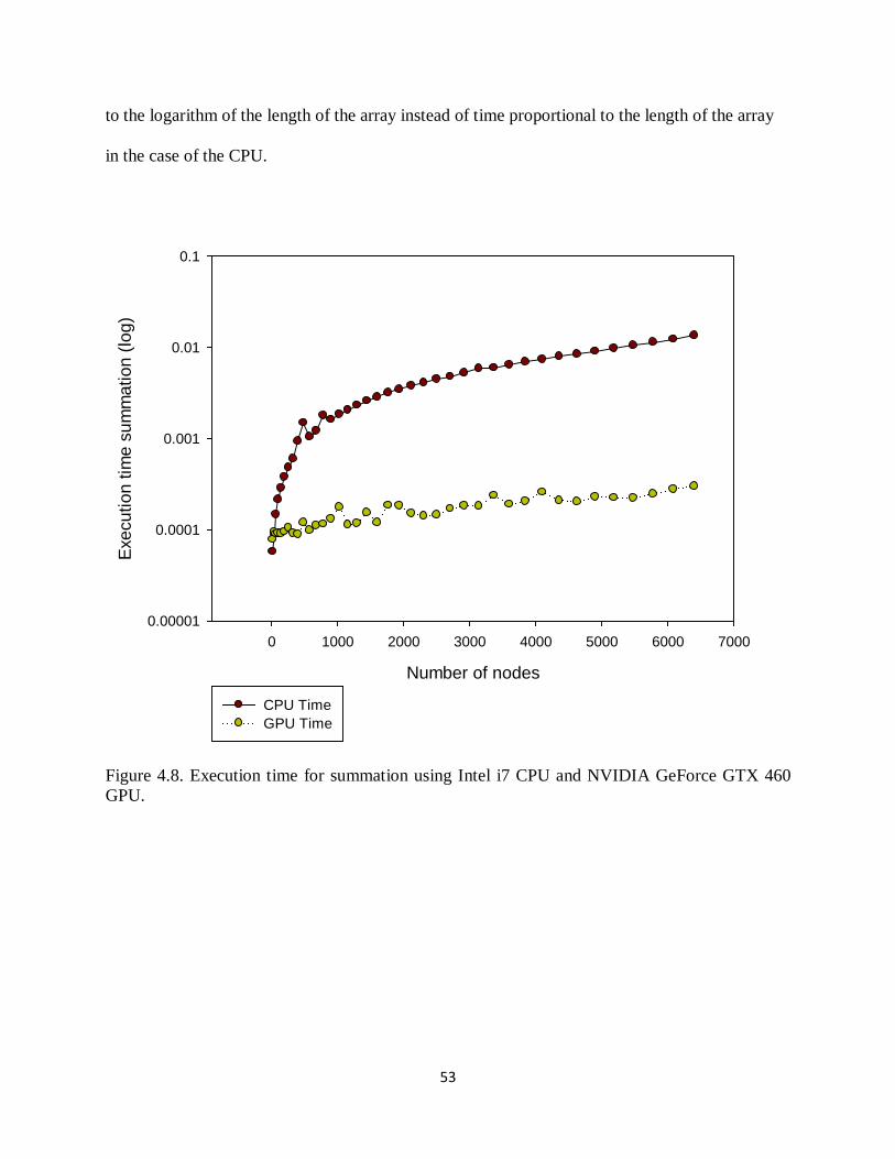
53

to the logarithm of the length of the array instead of time proportional to the length of the array

in the case of the CPU.

Number of nodes

0 1000 2000 3000 4000 5000 6000 7000

Exec

utio

n tim

e su

mm

atio

n (lo

g)

0.00001

0.0001

0.001

0.01

0.1

CPU TimeGPU Time

Figure 4.8. Execution time for summation using Intel i7 CPU and NVIDIA GeForce GTX 460 GPU.

54

Number of nodes

0 1000 2000 3000 4000 5000 6000 7000

Spee

dup

Fact

or s

umm

atio

n

0

10

20

30

40

50

Speedup

Figure 4.9. Speedup for summation using Intel i7 CPU and NVIDIA GeForce GTX 460 GPU

The result obtained from the matrix solution is a good example of how to utilize GPU. In

figure 4.10, it can be observed that with the number of nodes less than 500, the CPU seems to be

faster than the GPU but the GPU outperforms the CPU as the number of nodes increase past 500.

It turns out that a massively parallel machine like a GPU tends to waste its resources and

therefore performs less when the number of data set is so small compared to the intensity of the

computation. The GPU provides more benefit when the reduction in computation time on the

GPU over the CPU exceeds the cost of the data transfer. Solving system of linear equations

55

ranges from O(n2) to O(n3) complexity. For a very small number of nodes (in this case less than

500), the computational complexity is not large enough to offset the cost of data transfer. But

clearly as the number of nodes become larger, the computational complexity offset the cost of

the data transfer.

Number of nodes

0 1000 2000 3000 4000 5000 6000 7000

Exec

utio

n Ti

me

mat

rix s

olut

ion

(log)

1e-5

1e-4

1e-3

1e-2

1e-1

1e+0

1e+1

1e+2

1e+3

CPU TimeGPU Time

Figure 4.10. Execution time for matrix solution using Intel i7 CPU and NVIDIA GeForce GTX 460 GPU.

The speedup for the matrix solution using Intel i7 CPU and NVIDIA GeForce GTX 460 GPU is shown in Figure 4.11. The GPU is about 60 times faster than the CPU.

56

Number of nodes

0 1000 2000 3000 4000 5000 6000 7000

Spee

dup

Fact

or m

atrix

sol

utio

n

0

20

40

60

80

Speedup

Figure 4.11. Speedup for matrix solution using Intel i7 CPU and NVIDIA GeForce GTX 460 GPU

57

Figure 4.12. Overall Execution time using Intel i7 CPU and NVIDIA GeForce GTX 460 GPU

58

Number of nodes

0 1000 2000 3000 4000 5000 6000 7000

Ove

rall

Spee

dup

fact

or

0

20

40

60

80

Speedup

Figure 4.13 Overall Speedup factor using Intel i7 CPU and NVIDIA GeForce GTX 460 GPU

Although the speedup results obtained using Intel i7 CPU and NVIDIA GeForce GTX

460 GPU were good, they seemed to be an outlier. This anomaly may be due to software update,

or a process running on the CPU background such that it made the CPU significantly slower

compared to the GPU. To remedy this problem, the execution testbed was then changed to Intel

i3 CPU @ 2.10 GHz (4 CPUs) for the C program and NVIDIA GeForce GT 525M for the

59

CUDA program. The results shows that the GPU execution was faster than the CPU. As the

number of nodes increased, the time it took to compute on the CPU increased significantly

(Figure 4.14 and 4.19).

Number of nodes

0 1000 2000 3000 4000 5000 6000 7000

Exec

utio

n Ti

me

Mat

rix fi

ll (L

og)

1e-4

1e-3

1e-2

1e-1

1e+0

1e+1

1e+2

CPUGPU

Figure 4.14. Execution time for matrix fill using Intel i3 CPU and NVIDIA GeForce GT 525M GPU.

60

Number of nodes

0 1000 2000 3000 4000 5000 6000 7000

Spee

dup

Fact

or m

atrix

fill

0

2

4

6

8

10

12

14

Speedup

Figure 4.15. Speedup curve for matrix fill using Intel i3 CPU and NVIDIA GeForce GT 525M GPU.

61

Number of nodes

0 1000 2000 3000 4000 5000 6000 7000

Exec

utio

n Ti

me

Sum

mat

ion

(log

)

0.0001

0.001

0.01

0.1

CPUGPU

Figure 4.16. Execution time for summation of using Intel i3 CPU and NVIDIA GeForce GT 525M GPU.

62

Number of nodes

0 1000 2000 3000 4000 5000 6000 7000

Spee

dup

Fact

or S

umm

atio

n

0

2

4

6

8

10

12

14

16

18

20

Speedup

Figure 4.17. Speedup for summation using Intel i3 CPU and NVIDIA GeForce GT 525M GPU.

63

Number of nodes

0 1000 2000 3000 4000 5000 6000 7000

Exec

utio

n Ti

me

mat

rix s

olut

ion

(Log

)

1e-3

1e-2

1e-1

1e+0

1e+1

1e+2

CPUGPU

Figure 4.18. Execution time for matrix solution using Intel i3 CPU and NVIDIA GeForce GT 525M GPU.

64

Number of nodes

0 1000 2000 3000 4000 5000 6000 7000

Spee

dup

Fact

or m

atrix

sol

utio

n

0.0

0.5

1.0

1.5

2.0

2.5

Speedup

Figure 4.19 Speedup factor for matrix solution using Intel i3 CPU and NVIDIA GeForce GT 525M GPU.

65

Figure 4.20 Overall Execution time using Intel i3 CPU and NVIDIA GeForce GT 525M GPU.

As discussed earlier, the example problem was solved using the GPUs indicated and

various forms of the CPU reference program. For all results, the reference programs were run on

Intel Core i3 CPU @ 2.10 GHz. Results were collected and the values returned by each program

configuration were averaged over all trials.

First the matrix fill will be examined, followed by the summation, The measured speedup

which is defined in this research as the CPU time divided by GPU time is plotted for both GPUs

relative to the double precision i3 CPU and i7 CPU solvers as indicated.

66

Figure 4.21 Processing Time for Matrix Fill

0

200

400

600

800

1000

1200

1400

1600

i3 CPU i7 CPU GT 525M GTX 460

Aver

age

Proc

essi

ng ti

me

for m

atrix

fill

67

Figure 4.22 Processing Time for Summation

The computational result is in agreement with the analytical results for the example

problem solved, as shown in figure 4.23. The RMSE error was calculated as follows

=

−=∑100

2

1

( ) (8)

100i

Exact numRMSE

In the error computation, 100 nodes were used. All the nodes were specifically chosen

from within the interior of the domain. Because the meshless algorithm implemented results in a

non symmetric matrix, it will be inconsistent to compare solution derived from boundary nodes

to solution obtained from the interior nodes.

0

2

4

6

8

10

12

i3 CPU i7 CPU GT 525M GTX 460

Aver

age

Proc

essi

ng T

ime

for s

umm

atio

n

68

RMSE Analysis of CPU and GPU using Direct Solver

Number of nodes

0 1000 2000 3000 4000 5000 6000 7000

RM

SE

1.800e-3

2.000e-3

2.200e-3

2.400e-3

2.600e-3

2.800e-3

3.000e-3

3.200e-3

3.400e-3

3.600e-3

3.800e-3

CPU ErrorGPU Error

Figure 4.23. RMSE Analysis on the CPU and GPU

Second, a conjugate gradient method was pursued for use as the GaussianRBF matrix

equation solver. The conjugate gradient uses the value of the residual to compute a search vector

that is used to update the unknown. Each residual, therefore each search vector, is orthogonal to

the previous values. Theoretically, this means that the method will converge to the exact solution

when the number of iterations equals the number of unknowns [59]. The conjugate gradient

method is well suited to solving positive definite Hermetian systems. The Biconjugate method

69

(BiCG) on the other hand, can be applied to general matrix equations, but it lacks the

convergence properties of the former method. The BiCG replaces the orthogonal sequence above

with two sequences, one using the original matrix and one using its transpose, that are orthogonal

to each other [60]. A significant effect of this modification is that each iteration does not

necessarily reduce the residual and convergence becomes erratic. When using the BiCG method

exclusively for real symmetric global matrices, the method simplifies to the same structure of the

conjugate gradient method with the only difference being the use of different inner product, as

defined by the equations below. These inner products only differ by a single conjugate operation,

so that they are identical for real symmetric matrices.

Conjugate gradient: *

1

,n

i ii

f g f g=

=∑ (9)

Biconjugate gradient: 1

, .n

i ii

f g f g f g=

= =∑ (10)

The number of iterations required for convergence can be reduced by preconditioning,

which involves multiplying the matrix by the inverse of a new matrix (the preconditioner) in

order to reduce its condition number. This new matrix should approximate the original. In an

extreme case, if the original matrix is used as the preconditioner the equation will be solved in a

single iteration, but this would require inverting the global matrix, negating the need for an

iterative solver in the first place [59]. A Jacobi or diagonal preconditioner is a matrix containing

the main diagonal of the original array. Its inverse simply contains the reciprocals of the main

diagonal entries in their original locations. Pseudocode for the preconditioned BiCG method for

real symmetric matrices can be seen in [60] with the version used described in Figure 4.21

( where double brackets represent the Euclidean norm and is the convergence threshold)

70

Figure 4.24. Pseudo code of the Jacobi Preconditioned BiCG Method

𝑆𝑜𝑙𝑣𝑖𝑛𝑔 𝑨𝒙 = 𝒃

𝑰𝒏𝒊𝒕𝒊𝒂𝒍𝒊𝒛𝒆 𝒗𝒂𝒓𝒊𝒂𝒃𝒍𝒆𝒔:

𝑙𝑒𝑡 𝒙𝒐 = 0

𝑙𝑒𝑡 𝑴𝒊𝒊 =𝟏𝑨𝒊𝒊

𝒓𝒐 = 𝒃 − 𝑨𝒙𝒐 = 𝒃

𝒛𝒐 = 𝑴𝒓𝒐

𝒑𝒐 = 𝒛𝒐

𝑝𝑜 = 𝑟𝑜. 𝑧𝑜

𝑰𝒕𝒆𝒓𝒂𝒕𝒆 𝒇𝒓𝒐𝒎 𝒌 = 𝟏 𝒕𝒐 𝒎𝒂𝒙𝑰𝒕𝒆𝒓:

𝒒𝒌 = 𝑨𝒑𝒌−𝟏

𝜶𝒌 =𝒑𝒌−𝟏

𝒒𝒌.𝒑𝒌−𝟏

𝒙𝒌 = 𝒙𝒌−𝟏 + 𝜶𝒌𝒑𝒌−𝟏

𝒓𝒌 = 𝒓𝒌−𝟏 − 𝜶𝒌𝒒𝒌

𝒛𝒌 = 𝑴𝒓𝒌

𝑝𝑘 = 𝑟𝑘 . 𝑧𝑘

𝜷𝒌 =𝒑𝒌𝒑𝒌−𝟏

𝒑𝒌 = 𝒛𝒌 + 𝜷𝒌𝒑𝒌−𝟏

𝑩𝒓𝒆𝒂𝒌 𝑳𝒐𝒐𝒑 𝒊𝒇: ‖𝒓𝒌‖‖𝒃‖< 𝜖

71

A double precision BiCG solver was implemented on the CPU reference program as well

as the GPU. Using this solver requires less iteration to converge than the single precision solvers,

but each iteration requires significantly more computational time. The factors that limits a

particular routine depends on both the algorithm and hardware. The results in figures 4.24-4.27

shows the number of nodes (900) which reached the convergence threshold after 100 × number

of nodes on both the CPU and GPU

Number of nodes

0 200 400 600 800 1000

Exec

utio

n Ti

me

for s

umm

atio

n us

ing

BiC

G (l

og)

0.00001

0.0001

0.001

0.01

GPU CPU

Figure 4.25. Execution time for summation using BiCG solver

72

Number of nodes

0 200 400 600 800 1000

Spee

dup

Fact

or fo

r sum

mat

ion

0

2

4

6

8

10

12

Speedup

Figure 4.26. Speedup for summation using BiCG solver

73

Number of nodes

0 200 400 600 800 1000

Exec

utio

n Ti

me

mat

rix s

olut

ion

usin

g Bi

CG

(log

)

1e-4

1e-3

1e-2

1e-1

1e+0

1e+1

1e+2

1e+3

1e+4

1e+5

GPUCPU

Figure 4.27. Execution time for matrix solution using BiCG solver

74

Number of nodes

0 200 400 600 800 1000

Spee

dup

Fact

or m

atrix

sol

utio

n us

ing

BiC

G

0

1

2

3

4

5

6

Speedup

Figure 4.28. Speedup for matrix solution using BiCG solver

75

RMSE Analysis for CPU and GPU using BiCG Solver

Number of nodes

0 200 400 600 800 1000

RM

SE

0.0018

0.0020

0.0022

0.0024

0.0026

0.0028

0.0030

0.0032

0.0034

0.0036

0.0038

CPUGPU

Figure 4.29 RMSE Analysis for CPU and GPU using the Iterative Solver

In the future, more simulation will be conducted on GTX 480 and Quadro 2000 GPU to

justify the anomaly speedup obtained from the GTX 460.

76

LIMITATIONS

While the GaussianRBF CUDA kernel can handle relatively large data sets and provides

data coherence to the developer, it does have some limitations. CUDA has limitations on the

dimension of a grid. The maximum grid size for all existing Compute Capabilities is 65535 in

the X and Y dimensions. The maximum Z dimension is always 1. Therefore, an extremely large

input volume with row or plane axes greater than 65535 will cause the kernel to fail to run.

77

5. CONCLUSION

We have presented an application capable of utilizing the NVIDIA CUDA architecture to

solve a simple problem using a novel meshless method. A performance increase was

accomplished by implementing a matrix fill, direct solver, Biconjugate gradient solver, and

summation of matrix solution and RBFs on the GPU using the NVIDIA CUDA interface.

The project culminated in a program that solves the wave equation for a two dimensional

structure using the GaussianRBF. The program outputs the solution to the wave equation of the

rectangular structure. By examining a problem for which the analytical results could be easily

calculated, proper operation of the program was confirmed. In the performance tests, the

computational results were confirmed to be in agreement with analytical results.

While this program marks the endpoint of this research, it is expandable to serve as a

foundation for future work. Based on the framework of this project, options could be explored

including advanced solvers, modifying or using different method that is better conditioned to

solve the PDE. With the recent manufacturer investments and growing popularity of these

techniques in the developer community, this work should be viable for years to come.

78

LIST OF REFERENCES

79

6. REFERENCES

1.http://developer.download.nvidia.com/compute/DevZone/docs/html/C/doc/CUDA_C_Programming_Guide.pdf.

2.http://developer.download.nvidia.com/compute/DevZone/docs/html/C/doc/CUDA_C_Programming_Guide.pdf.

3.http://developer.download.nvidia.com/compute/DevZone/docs/html/C/doc/CUDA_C_Programming_Guide.pdf.

4.http://www.nvidia.com/content/PDF/fermi_white_papers/NVIDIAFermiComputeArchitectureWhitepaper.pdf.

5. ATI CTM Guide. (2007), http://www.cct.lsu.edu/~scheinin/Parallel/R600_ISA.pdf

6. Proceedings - DSD'2005: 8th Euromicro Conference on Digital System Design - Architectures, Methods and Tools 2005, 306 (2005).

7. ATI RADEON HD 4800 SERIES, http://www.amd.com/us/products/desktop/graphics/ati-radeon-hd-4000/hd-4800/Pages/ati-radeon-hd-4800-overview.aspx.

8. Kruger J., Rudiger W., “Linear Algebra Operators for GPU Implementation of Numerical Algorithms”, In ACM Transactions on Graphics, 908-916, 2003.

9. Rumpf M., Strzodka R., “Using Graphics Cards for Quantized FEM Computations,” 2001.

10. Inman, M.J.; Elsherbeni, A.Z.; Maloney, J.G.; Baker, B.N.; , "GPU based FDTD solver with CPML boundaries," Antennas and Propagation Society International Symposium, 2007 IEEE , vol., no., pp.5255-5258, 9-15 June 2007

11. Baron, G.S.; Sarris, C.D.; Fiume, E. “Real-time S-MRTD simulation of electrically large indoor wireless channels with commodity GPUs”, Antennas and Propagation Society International Symposium 2006, IEEE.

12. Woolsey, M.; Hutchcraft, W.E.; Gordon, R.K.; , "High-Level programming of graphics hardware to increase performance of electromagnetics simulation," Antennas and Propagation Society International Symposium, 2007 IEEE , vol., no., pp.5925-5928, 9-15 June 2007

80

13. Zainud-Deen SH. “Electromagnetic scattering using gpu-based finite difference frequency domain method”. Progress in electromagnetics research. Research B. 2009;16:351-369.

14. NVIDIA'S 1.4 BILLION TRANSISTOR GPU, http://www.anandtech.com/show/2549.

15. http://graphics.stanford.edu/projects/gpubench/.

16. http://developer.amd.com/tools/cpu/acml/onlinehelp/Documents/index.html.

17. - Hardy, R. L. - Multiquadric Equations of Topography and Other Irregular Surfaces. - J. Geophys. Res., - 1905.

18. Ala, G. G. A smoothed particle interpolation scheme for transient electromagnetic simulation. IEEE Trans. Magn. 42, 647-650 (2006).

19. Atluri, S. N., Kim, H. -. & Cho, J. Y. A critical assessment of the truly Meshless Local Petrov-Galerkin (MLPG), and Local Boundary Integral Equation (LBIE) methods. Computational Mechanics 24, 348-372 (1999).

20. Atluri, S. N., Sladek, J., Sladek, V. & Zhu, T. The local boundary integral equation (LBIE) and it's meshless implementation for linear elasticity. Computational Mechanics 25, 180-198 (2000).

21. Atluri, S. N. & Zhu, T. A new Meshless Local Petrov-Galerkin (MLPG) approach in computational mechanics. Computational Mechanics 22, 117-127 (1998).

22. Atluri, S. N. & Zhu, T. -. The meshless local Petrov-Galerkin (MLPG) approach for solving problems in elasto-statics. Computational Mechanics 25, 169-179 (2000).

23. Atluri, S. N. & Zhu, T. New concepts in meshless methods. Int J Numer Methods Eng 47, 537-556 (2000).

24. http://crd.lbl.gov/~dhbailey/mpdist.

25. Bakhoda, A., Yuan, G. L., Fung, W. W. L., Wong, H. & Aamondt, T. M. Analyzing CUDA workloads using a detailed GPU simulator (In 2009 IEEE InternationalSymposium on Performance Analysis of Systems and Software (ISPASS), 2009).

26. Barrett, R. in Templates for the solution of linear systems : building blocks for iterative methods (SIAM, Philadelphia, 1994).

81

27. Belytschko, T., Lu, Y. Y. & Gu, L. Element-free Galerkin methods. Int J Numer Methods Eng 37, 229-256 (1994).

28. Caldora Costa, M. M. An adaptive method applied to the diffuse element approximation in optimization process. IEEE Trans. Magn. 37, 3418-3422 (2001).

29. Costa, M. C. M. C. Optimisation of a switched reluctance motor using experimental design method and diffuse elements response surface. IEE proceedings.Science, measurement and technology 151, 411 (2004).

30. Franke, R. Scattered data interpolation: Tests of some methods. Mathematics of computation 38, 181 (1982).

31. Gingold, R. A. & Moraghan, J. J. Smoothed particle hydrodynamics; theory and applications to non-spherical stars. Monthly Notices of the Royal Astronomical Society 181, 375-389 (1977).

32. Gordon, R. R. K. Two approaches for the numerical determination of electromagnetic fields near material interfaces using radial basis functions in a meshless method. Numerical methods for partial differential equations 26, NA-NA (2009).

33. Ho, S. L. S. L. A Meshless Collocation Method Based on Radial Basis Functions and Wavelets. IEEE Trans. Magn. 40, 1021-1024 (2004).

34. Jiang, P. P. L. Analysis of elliptical waveguides by a meshless collocation method with the Wendland radial basis functions. Microwave Opt Technol Lett 32, 162-165 (2002).

35. Kansa, E. J. E. J. Multiquadrics—A scattered data approximation scheme with applications to computational fluid-dynamics—I surface approximations and partial derivative estimates. Computers & mathematics with applications (1987) 19, 127-145 (1990).

36. Kansa, E. J. E. J. Multiquadrics—A scattered data approximation scheme with applications to computational fluid-dynamics—II solutions to parabolic, hyperbolic and elliptic partial differential equations. Computers & mathematics with applications (1987) 19, 147-161 (1990).

37. Kim, D. D. W. Point collocation methods using the fast moving least-square reproducing kernel approximation. Int J Numer Methods Eng 56, 1445-1464 (2003).

38. Liszka, T. J., Duarte, C. A. M. & Tworzydlo, W. W. hp-Meshless cloud method. Comput. Methods Appl. Mech. Eng. 139, 263-288 (1996).

82

39. Liu, G. R. (. in Mesh free methods : moving beyond the finite element method 692 p. : (CRC Press, Boca Raton, Fla. :, 2003).

40. Liu, S. S. Improvement of the Element-Free Galerkin Method for Electromagnetic Field Calculation. IEEE Trans. Appl. Supercond. 14, 1866-1869 (2004).

41. Liu, W. K., Jun, S. & Zhang, Y. F. Reproducing kernel particle methods. Int. J. Numer. Methods Fluids 20, 1081-1106 (1995).

42. Marechal, Y. Y. Use of the diffuse element method for electromagnetic field computation. IEEE Trans. Magn. 29, 1475-1478 (1993).

43. Ni, G. Meshless local Petrov-Galerkin method and its application to electromagnetic field computations. Int. J. Appl. Electromagn. Mech. 19, 111 (2004).

44. OÑATE, E., IDELSOHN, S., ZIENKIEWICZ, O. C. & TAYLOR, R. L. A FINITE POINT METHOD IN COMPUTATIONAL MECHANICS. APPLICATIONS TO CONVECTIVE TRANSPORT AND FLUID FLOW. Int J Numer Methods Eng 39, 3839-3866 (1996).

45. Owens, J. D. et al. GPU Computing. Proceedings of the IEEE 96, 879-899 (2008).

46. Sanders, J. in CUDA by example : an introduction to general-purpose GPU programming p.7-12 (Addison-Wesley, Upper Saddle River, NJ :, 2011).

47. http://reference.kfupm.edu.sa/content/i/n/an_introduction_to_the_conjugate_gradient_55475.pdf.

48. Shiyou Yang, J. R. S. A combined wavelet-element free galerkin method for numerical calculations of electromagnetic fields. IEEE Trans. Magn. 39, 1413-1416 (2003).

49. Taflove, A. in Computational electrodynamics : the finite-difference time-domain method (Artech House, Boston Mass. [u.a.], 2000).

50. Viana, S. A. S. A. Meshless local Petrov–Galerkin method with radial basis functions applied to electromagnetics. IEE proceedings.Science, measurement and technology 151, 449 (2004).

51. Viana, S. A. S. A. Meshless local Petrov–Galerkin method with radial basis functions applied to electromagnetics. IEE proceedings.Science, measurement and technology 151, 449 (2004).

52. Viana, S. A. S. A. Moving least square reproducing kernel method for electromagnetic field computation. IEEE Trans. Magn. 35, 1372-1375 (1999).

83

53. Volakis, J. in Finite element method electromagnetics : antennas, microwave circuits, and scattering applications (Wiley-IEEE, Piscataway, NJ :, 1998).

54. Wong, A. S. M. A. S. M. Multizone decomposition for simulation of time-dependent problems using the multiquadric scheme. Computers & mathematics with applications (1987) 37, 23-43 (1999).

55. Xuan, L. Element-free Galerkin method in pulsed eddy currents. Int. J. Appl. Electromagn. Mech. 19, 463 (2004).

56. Xuan, L. L. Element-Free Galerkin Method for Static and Quasi-Static Electromagnetic Field Computation. IEEE Trans. Magn. 40, 12-20 (2004).

57. Zhao Meiling, N. Y. A new coupled MLPG-FE method for electromagnetic field computations. Computational Electromagnetics and Its Applications, Proceedings, ICCEA, International Conference on, 29-32 (2004).

58. Zhu, T., Zhang, J. -. & Atluri, S. N. A local boundary integral equation (LBIE) method in computational mechanics, and a meshless discretization approach. Computational Mechanics 21, 223-235 (1998).

59. Zongmin, W. Hermite-Birkhoff interpolation of scattered data by radial basis functions. Approximation Theory and its Applications 8, 1-10 (1992).

60. Jin, J. The Finite Element Method in Electromagnetics. 2nd ed. New York: Wiley, 2002

61. Barrett R., Berry M., Chan T.F., Demmel J., Donato J.M., Dongarra J., Eijkhout V., Pozo R., Romine C., Van der Vorst H., Templates for the Solution of Linear Systems: Building Blocks for Iterative Methods 2nd ed. s.l.: Society for Industrial and Applied Mathematics, 1993.

84

LIST OF APPENDICES

85

7. APPENDICES

Appendix A Compute capabilities of CUDA enabled GPUs ……………….71

Appendix B How to configure Visual C++ to run CUDA program…………72

86

APPENDIX A: COMPUTE CAPABILITY OF CUDA ENABLED GPUS

87

88

APPENDIX B: HOW TO CONFIGURE VISUAL C++ TO RUN CUDA PROGRAM

89

1. Open Visual C++ and Select File > New > Project

2. Select Win32 under Project types and Win32 Console Application under Visual Studio

installed templates.

3. Enter in the name of your project and select OK

4. When the wizard pops up select Next, then check Empty project and select Finish.

90

5. Right click on your project and select Custom Build Rules.

6. If there is a CUDA Build Rules listed then go to step 10, otherwise continue to step 7.

7. Select New Rule File…

8. In the Display Name box put CUDA Build Rules, for File Name put the name of the file

(usually cuda.rules), and then for Directory browse to the CUDA rules file on the machine.

9. Once that is complete select Add Build Rule… and press OK.

10. Check the CUDA Build Rules listed under Available Rule Files and select OK.

11. Now you should be able to add your header, resources, and source files in their

respective folders.

Note: It may be easier to locate the Template.sln file on your machine under the sample

NVIDIA projects and use that as a starting point to write your program. This project is already

configured and all you would have to do is add your files.

91

8. VITA

Derek Owusu-Banson was born in Takoradi, Western Region of Ghana. He graduated from

St Augustine’s College in Cape Coast, Central Region of Ghana in 2003. During this time he was

a member of the school’s Science and Math Quiz Team. After graduating from high school, he

worked for the then Ghana Telecommunications Company as phone cards whole sale distributor.

In Spring 2005, he enrolled in the University of Mississippi in Oxford, Mississippi of United

States. During his undergraduate period, he worked part-time on campus doing technical support

for the University of Mississippi Housing Department. During this time, he also worked for the

Material Handling branch of FMC in tupelo, where he was involved in the light electromagnetic

feeder research and development projects. He also worked at the National Center for Physical

Acoustics in Oxford, where he researched and implemented a new method of characterizing

acoustic anechoic chambers. He received the degree of Bachelor of Science in Electrical

Engineering with Emphasis in Computer Engineering from the University of Mississippi in

December 2009. In August 2010, he entered the Graduate School at the University of

Mississippi. During this time he worked on accelerating the performance of a new meshless

method by utilizing the GPU as a parallel co-processor.

92