Embed Size (px)
Citation preview

Chapter 12
Fourier Series
Just before 1800, the French mathematician/physicist/engineer Jean Baptiste JosephFourier made an astonishing discovery. As a result of his investigations into the partial dif-ferential equations modeling vibration and heat propagation in bodies, Fourier was led toclaim that “every” function could be represented by an infinite series of elementary trigono-metric functions — sines and cosines. As an example, consider the sound produced by amusical instrument, e.g., piano, violin, trumpet, oboe, or drum. Decomposing the signalinto its trigonometric constituents reveals the fundamental frequencies (tones, overtones,etc.) that are combined to produce its distinctive timbre. The Fourier decomposition liesat the heart of modern electronic music; a synthesizer combines pure sine and cosine tonesto reproduce the diverse sounds of instruments, both natural and artificial, according toFourier’s general prescription.
Fourier’s claim was so remarkable and unexpected that most of the leading mathe-maticians of the time did not believe him. Nevertheless, it was not long before scientistscame to appreciate the power and far-ranging applicability of Fourier’s method, therebyopening up vast new realms of physics, engineering, and many other fields, to mathematicalanalysis. Indeed, Fourier’s discovery easily ranks in the “top ten” mathematical advancesof all time, a list that would include Newton’s invention of the calculus and Riemann’sestablishment of differential geometry that, 70 years later, became the foundation of Ein-stein’s general relativity. Fourier analysis is an essential component of much of modernapplied (and pure) mathematics. It forms an exceptionally powerful analytical tool forsolving a broad range of partial differential equations. Applications in pure mathematics,physics and engineering are almost too numerous to catalogue — typing in “Fourier” inthe subject index of a modern science library will dramatically demonstrate just how ubiq-uitous these methods are. For instance, modern signal processing, including audio, speech,images, videos, seismic data, radio transmissions, and so on, is based on Fourier analysis.Many modern technological advances, including television, music CD’s and DVD’s, videomovies, computer graphics, image processing, and fingerprint analysis and storage, are, inone way or another, founded upon the many ramifications of Fourier’s discovery. In yourcareer as a mathematician, scientist or engineer, you will find that Fourier theory, like cal-culus and linear algebra, is one of the most basic and essential tools in your mathematicalarsenal. Mastery of the subject will be unavoidable.
In addition, a remarkably large fraction of modern pure mathematics is the result ofsubsequent attempts to place Fourier series on a firm mathematical foundation. Thus,all of the student’s “favorite” analytical tools, including the modern definition of a func-tion, the ε–δ definition of limit and continuity, convergence properties in function space,
2/25/04 465 c© 2004 Peter J. Olver
including uniform convergence, weak convergence, etc., the modern theory of integrationand measure, generalized functions such as the delta function, and many others, all owea profound debt to the prolonged struggle to establish a rigorous framework for Fourieranalysis. Even more remarkably, modern set theory, and, as a result, mathematical logicand foundations, can be traced directly back to Cantor’s attempts to understand the setsupon which Fourier series converge!
As we will appreciate, Fourier series are, in fact, a very natural outgrowth of the basiclinear algebra constructions that we have already developed for analyzing discrete dynam-ical processes. The Fourier representation of a function is a continuous counterpart of theeigenvector expansions used to solve linear systems of ordinary differential equations. Thefundamental partial differential equations governing heat propagation and vibrations incontinuous media can be viewed as the function space versions of such discrete systems. Inthe continuous realm, solutions are expressed as linear combinations of simple “separable”solutions constructed from the eigenvalues and eigenfunctions of an associated boundaryvalue problem. The efficacy of Fourier analysis in practice rests on the orthogonalityproperties of the trigonometric functions, which is a direct consequence of their status aseigenfunctions of the most basic self-adjoint boundary value problem. So, Fourier seriescan be rightly viewed as a function space version of the finite-dimensional spectral theoryof symmetric matrices and orthogonal eigenvector bases. The main complication is thatwe must now deal with infinite series rather than finite sums, and so convergence issuesthat do not appear in the finite-dimensional situation become of paramount importance.
Once we have established the proper theoretical background, the trigonometric Fourierseries will no longer be a special, isolated phenomenon, but, rather, in its natural context asthe simplest representative of a broad class of orthogonal eigenfunction expansions basedon self-adjoint boundary value problems. Modern and classical extensions of the Fouriermethod, including Fourier integrals, wavelets, discrete Fourier series, Bessel functions,spherical harmonics, as well as the entire apparatus of modern quantum mechanics, all reston the same basic theoretical foundation, and so gaining familiarity with the general theoryand abstract eigenfunction framework will be essential. Many of the most important casesused in modern physical and engineering applications will appear in the ensuing chapters.
We begin our development of Fourier methods with a section that will explain whyFourier series naturally appear when we move from discrete systems of ordinary differen-tial equations to the partial differential equations that govern the dynamics of continuousmedia. The reader uninterested in motivations can safely omit this section as the samematerial reappears in Chapter 14 when we completely analyze the dynamical partial differ-ential equations that lead to Fourier methods. Beginning in Section 12.2, we shall review,omitting proofs, the most basic computational techniques in Fourier series, for both ordi-nary and generalized functions. In the final section, we include an abbreviated introductionto the analytical background required to develop a rigorous foundation for Fourier seriesand their convergence.
12.1. Dynamical Equations of Continuous Media.
In continuum mechanics, systems of discrete masses and springs are replaced by con-tinua, e.g., one-dimensional bars and strings, two-dimensional plates and membranes or
2/25/04 466 c© 2004 Peter J. Olver
three-dimensional solid bodies. Of course, real physical bodies are composed of atoms,and so could, at least in principle, be modeled by discrete mechanical systems. However,the number of atoms is so large that any direct attempt to analyze the resulting system ofordinary differential equations would be completely impractical. Thus, regarding bodies asideal continuous media not only leads to very accurate physical models, but is absolutelycrucial for significant progress towards their mathematical and computational analysis.Paradoxically, the numerical solution of such partial differential equations returns us tothe discrete realm, but now in a computationally tractable form. While one might envisiongoing directly from the discrete atomic system to the discrete numerical approximation,this is not a simple matter. The analytical power and insight offered by calculus in thecontinuous regime makes this intermediate construction an essential component for theeffective modeling of physical phenomena.
As we saw in Chapter 6, the equilibrium configurations of discrete mechanical systemsare found by solving a linear algebraic systemKu = f with positive (semi-)definite stiffnessmatrix for the displacement vector u. In Chapter 11, we learned that the same abstractformalism applies to the equilibrium equations of one-dimensional media — bars, beams,etc. The solution is now a function u(x) representing, say, displacement or temperature ofthe bar, while the linear matrix system is replaced by a positive (semi-)definite boundaryvalue problem K[u ] = f involving a linear ordinary differential equation supplemented bya suitable collection of boundary conditions.
In Chapter 9, we studied the dynamics of discrete systems, which are governed by ini-tial value problems for linear systems of ordinary differential equations. The two principalclasses that were treated are the first order systems (9.22) governing gradient flows, andthe second order Newtonian vibration systems (9.54). Let us first consider the unforcedgradient flow system
du
dt= −Ku, u(t0) = u0, (12.1)
associated with the positive (semi-)definite coefficient matrix K. Gradient flows are de-signed to decrease the quadratic energy function q(u) = 1
2 uTKu as rapidly as possible.
By analogy, in a continuum, a (linear) gradient flow will be a partial differential equationfor a function u(t, x) depending upon time and spatial position and taking the general,abstract form
∂u
∂t= −K[u ], u(t0, x) = f(x), (12.2)
in which the differential operator K is supplemented by the same equilibrium spatialboundary conditions. Such partial differential equations model diffusion processes in whicha quadratic energy functional is decreasing as rapidly as possible. A good physical exampleis the flow of heat in a body in which u(t, x) represents the temperature at time t andposition x. Heat disperses throughout the body so as to decrease the thermal energy as fastas it can, tending (in the absence of external heat sources) to thermal equilibrium. Otherphysical processes modeled by (12.2) include diffusion of chemicals (solvents, pollutants,etc.), and of populations (animals, bacteria, people, etc.).
The simplest and most instructive example is the case of a uniform periodic (or cir-cular) bar of length 2π. As we saw in Chapter 11, the equilibrium equation for the
2/25/04 467 c© 2004 Peter J. Olver
temperature u(x) takes the form
K[u ] = −u′′ = f, u(−π) = u(π), u′(−π) = u′(π), (12.3)
associated with the positive semi-definite differential operator
K = D∗ ◦D = (−D)D = −D2 (12.4)
acting on the space of 2π periodic functions. The corresponding gradient flow (12.2) is thepartial differential equation
∂u
∂t=
∂2u
∂x2, u(t,−π) = u(t, π),
∂u
∂x(t,−π) = ∂u
∂x(t, π), (12.5)
known as the heat equation. A physical derivation of (12.5) will appear in Chapter 14.The solution to (12.5) is uniquely prescribed by the initial temperature distribution,
u(0, x) = f(x), −π ≤ x ≤ π. (12.6)
Solving the initial-boundary value problem (12.5)perheaticn for the periodic heat equationwas the seminal problem that led Fourier to develop the profound theory that now bearshis name.
Now, to solve a finite-dimensional system of ordinary differential equations such as(12.1), we sought solutions of pure exponential form u(t) = e−λtv. The net effect wasto reduce the differential equation to the eigenvector equation Kv = λv for the stiffnessmatrix K. The general solution was then realized as a linear superposition of the basiceigensolutions. This same idea carries over directly to the continuous realm! To findthe basic solutions to the partial differential equation (12.2), we postulate an exponentialformula
u(t, x) = e−λt v(x), (12.7)
in which the function v(x) assumes the role of the eigenvector v. Since v doesn’t dependon t,
∂u
∂t=
∂
∂t
[e−λt v(x)
]= −λ e−λt v(x),
while
−K[u ] = −K[e−λt v(x)
]= −e−λtK[v ],
since the linear operator K only involves differentiation with respect to x and so doesn’taffect the exponential factor. Substituting these two expressions into the dynamical equa-tions (12.2) and canceling the common exponential factor, we conclude that v(x) mustsolve the ordinary differential equation
K[v ] = λ v. (12.8)
Moreover, to guarantee that our exponential formula (12.7) defines a solution, we mustalso require that v(x) satisfy the relevant boundary conditions, and hence (12.8) consti-tutes a boundary value problem for v(x). We interpret λ as the eigenvalue and v(x) as the
2/25/04 468 c© 2004 Peter J. Olver

corresponding eigenfunction for the operator K subject to the relevant boundary condi-tions. Each eigenvalue and eigenfunction pair will produce a solution (12.7) to the partialdifferential equation, and the general solution can be built up through linear superposition.
Returning to our example, substituting the exponential ansatz (12.7) into the periodicheat equation (12.5) leads to the eigenvalue problem
v′′ + λv = 0, v(−π) = v(π), v′(−π) = v′(π). (12.9)
for the eigenfunction v(x). Now, it is not hard to show that if λ < 0 or λ is complex, thenthe only periodic solution to (12.9) is the trivial solution v(x) ≡ 0. Thus, all eigenvaluesmust be real and non-negative: λ ≥ 0; in fact, this is a direct consequence of the fact,established in Section 11.3, that the underlying differential operator (12.4) is positive semi-definite when subject to periodic boundary conditions. When λ = 0, periodicity singlesout the nonzero constants v(x) ≡ c 6= 0 as the associated eigenfunctions. If λ = ω2 > 0,then the general solution to the differential equation (12.9) is
v(x) = a cosωx+ b sinωx. (12.10)
Assuming v(x) 6≡ 0, the 2π periodic boundary conditions require that ω = k is an inte-ger, in which case every nonzero solution to the differential equation is an eigenfunction.Therefore, the eigenvalues
λ = k2, 0 ≤ k ∈ N,
are the squares of positive integers. Each positive eigenvalue λ = k2 > 0 admits twolinearly independent eigenfunctions, namely sin kx and cos kx, while the zero eigenvalueλ = 0 has only one, the constant function 1. We conclude that the elementary trigonometricfunctions
1, cosx, sinx, cos 2x, sin 2x, cos 3x, . . . (12.11)
form a complete system of independent eigenfunctions for the periodic boundary valueproblem (12.9).
By construction, each eigenfunction gives rise to a particular solution (12.7) to theperiodic heat equation (12.5). We have therefore discovered an infinite collection of inde-pendent solutions:
uk(x) = e−k2 t cos kx, uk(x) = e−k2 t sin kx, k = 0, 1, 2, 3, . . . .
Linear superposition tells us that linear combinations of solutions are also solutions, andso we are inspired to try an infinite series†
u(t, x) =a0
2+
∞∑
k=1
[ak e
−k2 t cos kx+ bk e−k2 t sin kx
](12.12)
† For technical reasons, one takes the basic null eigenfunction to be 12 instead of 1. The
explanation will be revealed in the following section.
2/25/04 469 c© 2004 Peter J. Olver

to represent the general solution to the periodic heat equation. (Of course, the super-position principle only applies without qualification to finite sums, but let us ignore this“technicality” for a moment.) As in the discrete version, the coefficients ak, bk are foundby substituting the solution formula into the initial condition (12.6), whence
u(0, x) =a0
2+
∞∑
k=1
[ak cos kx+ bk sin kx
]= f(x). (12.13)
The result is the Fourier series representation of the initial temperature distribution. Oncewe have prescribed the Fourier coefficients ak, bk induced by f(x), we will then have anexplicit formula for the solution to the periodic initial-boundary value problem for the heatequation.
However, since we are dealing with infinite series, the preceding solution is purelya formal construction, and sorely in need of some serious analysis to place it on a firmfooting. The key questions are
• First, when does such an infinite trigonometric series converge?• Second, what kinds of functions f(x) can be represented by a convergent Fourier series?• Third, if we have such an f , how do we determine its Fourier coefficients ak, bk?• And lastly, since we are trying to solve differential equations, can we safely differentiate
a Fourier series?
Without some serious analysis, we will be unable to ascertain the full scope of the Fourierseries method for our chosen applications. The bulk of this chapter will be devoted towardanswering these fundamental questions. Once we have acquired a firm foundation in thebasics of Fourier theory, we can then return, in Chapter 14, to establish the validity of ourFourier series solution and discover what it tells us about the quantitative and qualitativeproperties of the dynamical solutions to the heat equation.
A similar analysis applies to the partial differential equations governing the dynamicalmotions of continuous media. Recall, (9.54), that the free vibrations of a discrete mechan-ical system are governed by a second order system of ordinary differential equations of theform†
d2u
dt2= −Ku
with symmetric, positive (semi-)definite stiffness matrix K. In the continuous realm,Newton’s laws of motion lead to a second order partial differential equation of the analogousform
∂2u
∂t2= −K[u ], (12.14)
in which the solution u(t, x) measures displacement at time t and position x and K rep-resents the same self-adjoint differential operator, supplemented by appropriate boundary
† We are ignoring the effects of variable mass or density in the current simplified discussion.Density effects will be included in the continuous models when we return to a more detaileddevelopment in Section 14.4.
2/25/04 470 c© 2004 Peter J. Olver
conditions, that appears in the corresponding equilibrium boundary value problem. SuchNewtonian systems are used to describe the free vibrations of continuous mechanical sys-tems, such as bars, beams, and, in higher dimensions, membranes and solid bodies. Theyalso arise in the propagation of electromagnetic and light waves, water waves and otherfluid vibrations, and many other physical systems. In particular, the equation (12.14)induced by the simplest self-adjoint differential operator (12.4) is the wave equation
∂2u
∂t2=
∂2u
∂x2, (12.15)
which models stretching vibrations of a bar, sound vibrations in a column of air, e.g., insidea wind instrument, and the transverse vibrations of a string, e.g., on a violin or piano.
To proceed, we must also impose suitable boundary conditions. Consider, for example,the wave equation with homogeneous Dirichlet boundary conditions
∂2u
∂t2=
∂2u
∂x2, u(t, 0) = 0, u(t, `) = 0, (12.16)
that models, for instance, the vibrations of a uniform violin string whose ends are tied down.In the discrete matrix ordinary differential equation, we used a trigonometric ansatz of theform cos(ωt)v to find the basic solutions. By analogy, we look for a separable solution ofthe form
u(t, x) = cos(ωt) v(x) (12.17)
in which ω represents the vibrational frequency. Substituting (12.17) into the wave equa-tion and the boundary conditions, we deduce that v(x) must be a solution to the boundaryvalue problem
d2v
dx2+ ω2 v = 0, v(0) = 0 = v(`), (12.18)
in which ω2 = λ plays the role of the eigenvalue. If ω2 is either complex, or non-positive,ω2 ≤ 0, then the boundary value problem only admits the trivial solution v(x) ≡ 0, andso all the eigenvalues are strictly positive, which is, in fact, a consequence of positivedefiniteness. When ω2 > 0, the general solution to the differential equation is, as before,
v(x) = a cosωx+ b sinωx.
The boundary condition at x = 0 requires a = 0, and so
v(x) = b sinωx.
The second boundary condition requires
v(`) = b sinω` = 0.
Assuming b 6= 0, as otherwise the solution is trivial, ω` = kπ must be an integer multipleof π. Thus, the natural frequencies of vibration are
ωk =kπ
`, k = 1, 2, 3, . . . .
2/25/04 471 c© 2004 Peter J. Olver
The corresponding eigenfunctions are
vk(x) = sink π x
`, k = 1, 2, 3, . . . , (12.19)
resulting in the following natural modes of vibration for the wave equation:
uk(t, x) = coskπ t
`sin
kπx
`, uk(t, x) = sin
kπ t
`sin
kπx
`.
Each solution represents a spatially periodic standing wave form. We expect to be able towrite the general solution to the boundary value problem as an infinite series
u(t, x) =∞∑
k=1
(bk cos
kπ t
`sin
kπx
`+ dk sin
kπ t
`sin
kπx
`
)(12.20)
in the natural modes. The coefficients bk, dk will be determined by the initial conditions.At each fixed t, the solution assumes the form of a Fourier series in which only the sineterms appear. Again, we must deal with the same convergence issues in order to ascertainthe validity of this solution formula.
We have now completed our brief introduction to the dynamical equations of continu-ous media and the Fourier series method of solution. The student should now be sufficientlymotivated, and it is time to delve into the theory of basic Fourier series. We will not try todeal with more general eigenfunction expansions until much later, in Chapter 17, but beginby concentrating on the simplest and most important special case, when the eigenfunctionsare trigonometric, and the series is a classical Fourier series. In Chapter 14 we will applywhat we learn to study the one-dimensional heat and wave equations in depth.
12.2. Fourier Series.
The preceding section served as a launching pad to motivate Fourier analysis. Webegin the discussion with the basic definition.
Definition 12.1. A Fourier series is an infinite trigonometric series
f(x) ∼ a0
2+
∞∑
k=1
[ ak cos kx+ bk sin kx ] . (12.21)
The extra factor of 12 is traditionally included in the first term for later convenience.
Of course, without additional assumptions on the coefficients ak, bk, the Fourier series(12.21) may not converge. This is the reason that we use the ∼ symbol instead of an equalssign.
The first order of business is to determine the formulae for the Fourier coefficientsak, bk. The key is orthogonality. We already observed, in Example 5.12, that the trigono-metric functions are orthogonal with respect to the (rescaled) L2 inner product
〈 f ; g 〉 = 1π
∫ π
−πf(x) g(x) dx (12.22)
2/25/04 472 c© 2004 Peter J. Olver

on the interval† [−π, π ]. The explicit orthogonality relations are
〈 cos kx ; cos l x 〉 = 〈 sin kx ; sin l x 〉 = 0,〈 cos kx ; sin l x 〉 = 0,
‖ 1 ‖ =√2 , ‖ cos kx ‖ = ‖ sin kx ‖ = 1,
for k 6= l,
for all k, l,
for k 6= 0,(12.23)
where k and l indicate non-negative integers.
Remark : If we were to replace the constant function 1 by 1√2, then the resulting
functions would form an orthonormal system. However, this extra√2 factor turns out to
be utterly annoying, and is best omitted from the outset.
If we ignore convergence issues for the moment and treat the Fourier series represen-tation (12.21) as an equality, then the orthogonality relations (12.23) serve to immediatelydetermine the Fourier coefficients. Taking the inner product of both sides with, respec-tively, cos kx and sin kx, we find
ak = 〈 f ; cos kx 〉 =1
π
∫ π
−πf(x) cos kx dx, k = 0, 1, 2, 3, . . . ,
bk = 〈 f ; sin kx 〉 =1
π
∫ π
−πf(x) sin kx dx, k = 1, 2, 3, . . . .
(12.24)
These fundamental formulae prescribe the Fourier coefficients of the function f . The factthat we can also use them as written for a0 is the reason for including the
12 in the constant
term of the Fourier series (12.21).
Example 12.2. Consider the function f(x) = x. We may compute its Fouriercoefficients directly, using integration by parts to evaluate the integrals:
a0 =1
π
∫ π
−πx dx = 0, ak =
1
π
∫ π
−πx cos kx dx =
1
π
[x sin kx
k+cos kx
k2
] ∣∣∣∣π
x=−π= 0,
bk =1
π
∫ π
−πx sin kx dx =
1
π
[− x cos kx
k+sin kx
k2
] ∣∣∣∣π
x=−π=2
k(−1)k+1 . (12.25)
Therefore, the Fourier cosine coefficients of the function x all vanish, ak = 0, and itsFourier series is
x ∼ 2
(sinx − sin 2x
2+sin 3x
3− sin 4x
4+ · · ·
). (12.26)
The convergence of this series is not an elementary matter. Standard tests, including theratio and root tests, that almost always work for power series, fail to apply. Even if we
† We have chosen the interval [−π, π ] for convenience. A common alternative is the interval[0, 2π ]. In fact, since the trigonometric functions are 2π periodic, any interval of length 2πwill serve equally well. Adapting Fourier series to intervals of other lengths will be discussed inSection 12.4.
2/25/04 473 c© 2004 Peter J. Olver

know that the series converges (which it does, for all x) it is certainly not obvious whatfunction it converges to. Indeed, it cannot converge to the function f(x) = x for all valuesof x. If we substitute x = π, then every term in the series is zero, and so the Fourier seriesconverges to 0 — which is not the same as f(π) = π.
The nth partial sum of a Fourier series is the trigonometric polynomial†
sn(x) =a0
2+
n∑
k=1
[ ak cos kx+ bk sin kx ] . (12.27)
Thus, the Fourier series converges at a point x if and only if the partial sums have a limit
limn→∞
sn(x) = f(x), (12.28)
which may or may not equal the value of the original function f(x). Thus, a key require-ment is to formulate easily verifiable conditions on the function f(x) that guarantee thatthe Fourier series converges, and, even more importantly, the limiting sum reproduces theoriginal function: f(x) = f(x). This will all be done in detail below.
Remark : The passage from trigonometric polynomials to Fourier series is analogousto the passage from polynomials to power series. A power series
f(x) ∼ c0 + c1 x+ · · · + cn xn + · · · =
∞∑
k=0
ck xk
can be viewed as an infinite linear combination of the basic monomials 1, x, x2, x3, . . . .
According to Taylor’s formula, (C.8), the coefficients ck =f (k)(0)
k!are given in terms of
the derivatives of the function at the origin. The partial sums
sn(x) = c0 + c1 x+ · · · + cn xn =
n∑
k=0
ck xk
of a power series are ordinary polynomials, and similar convergence issues arise.
Although superficially similar, in actuality the two theories are profoundly different. Apower series either converges everywhere, or on an interval centered at 0, or nowhere exceptat 0. (See Section 16.2 for additional details.) On the other hand, a Fourier series canconverge on quite bizarre sets. In fact, the detailed analysis of the convergence properties ofFourier series led Georg Cantor to formulate modern set theory, and, thus, played a seminalrole in the establishment of the foundations of mathematics. Secondly, when a powerseries converges, it converges to an analytic function, which is infinitely differentiable, andwhose derivatives are represented by the power series obtained by termwise differentiation.Fourier series may converge, not only to a periodic continuous function, but also to a wide
† The reason for the term “trigonometric polynomial” was discussed at length in Exam-ple 2.16(c).
2/25/04 474 c© 2004 Peter J. Olver

-5 5 10 15
-3
-2
-1
1
2
3
Figure 12.1. Periodic extension of x.
variety of discontinuous functions and, even, when suitably interpreted, to generalizedfunctions like the delta function! Therefore, the termwise differentiation of a Fourier seriesis a nontrivial issue. Indeed, while the theory of power series was well established in theearly days of the calculus, there remain, to this day, unresolved foundational issues inFourier theory.
Once one comprehends how different the two subjects are, one begins to understandwhy Fourier’s astonishing claims were initially widely disbelieved. Before the advent ofFourier, mathematicians only accepted analytic functions as the real thing. The fact thatFourier series can converge to nonanalytic, even discontinuous functions was extremelydisconcerting, and led to a complete re-evaluation of function theory, culminating in themodern definition of function that you now learn in first year calculus. Only through thecombined efforts of many of the leading mathematicians of the nineteenth century was arigorous theory of Fourier series firmly established.
Periodic Extensions
The trigonometric constituents (12.11) of a Fourier series are all periodic functions
of period 2π. Therefore, if the series converges, the resulting function f(x) must also beperiodic of period 2π:
f(x+ 2π) = f(x) for all x ∈ R.
A Fourier series can only converge to a 2π periodic function. Therefore, we should notexpect the Fourier series (12.26) to converge to f(x) = x everywhere, since it is not aperiodic function. Rather, it converges to its periodic extension, as we now define.
Lemma 12.3. If f(x) is any function defined for −π < x ≤ π, then there is a unique
2π periodic function f , known as the 2π periodic extension of f , that satisfies f(x) = f(x)for all −π < x ≤ π.
Proof : Pictorially, the graph of the periodic extension of a function f(x) is obtainedby repeatedly copying that part of the graph of f between −π and π to all other adjacentintervals of length 2π; see, for instance, Figure 12.1. More formally, given x ∈ R, there is
2/25/04 475 c© 2004 Peter J. Olver

a unique integer m so that −π < x− 2mπ ≤ π. Periodicity of f leads us to define
f(x) = f(x− 2mπ) = f(x− 2mπ).
In particular, if −π < x ≤ π, then m = 0 and hence f(x) = f(x). The proof that the
resulting function f is 2π periodic is left as Exercise . Q.E.D.
Remark : The construction of the periodic extension of Lemma 12.3 uses the valuef(π) at the right endpoint and requires f(−π) = f(π) = f(π). One could, alternatively,
require f(π) = f(−π) = f(−π), which, if f(−π) 6= f(π), leads to a slightly different 2πperiodic extension of the function, differing when x is an odd multiple of π. There is no apriori reason to prefer one over the other. In fact, for Fourier theory, as we shall discover,one should use neither, but rather an “average” of the two. Thus, the preferred Fourierperiodic extension f(x) will satisfy
f(π) = f(−π) = 12
[f(π) + f(−π)
], (12.29)
which then fixes its values at the odd multiples of π.
Example 12.4. The 2π periodic extension f(x) of f(x) = x is the “sawtooth”function graphed in Figure 12.1. It agrees with x between −π and π. If we adopt theFourier extension (12.29), then, for any odd integer k, we set f(kπ) = 0, the average ofthe values of f(x) = x at the endpoints ±π. Thus, explicitly,
f(x) =
{x− 2mπ, (2m− 1)π < x < (2m+ 1)π,
0, x = (2m− 1)π, where m is an arbitrary integer.
With this convention, it can be proved that the Fourier series (12.26) for f(x) = x converges
everywhere to the 2π periodic extension f(x). In particular,
2∞∑
k=1
(−1)k+1 sin kx
k=
{x, −π < x < π,
0, x = ±π. (12.30)
Even this very simple example has remarkable and nontrivial consequences. For in-stance, if we substitute x = 1
2 π in (12.26) and divide by 2, we obtain Gregory’s series
π
4= 1 − 1
3+1
5− 1
7+1
9− · · · . (12.31)
While this striking formula predates Fourier theory — it was first discovered by Leibniz— a direct proof is not easy.
Remark : While fascinating from a numerological viewpoint, Gregory’s series is ofscant practical use for actually computing π since its rate of convergence is painfullyslow. The reader may wish to try adding up terms to see how far out one needs to go toaccurately compute even the first two decimal digits of π. Round-off errors will eventuallyinterfere with any attempt to compute the complete summation to any reasonable degreeof accuracy.
2/25/04 476 c© 2004 Peter J. Olver
-1 1 2 3 4
-1
-0.5
0.5
1
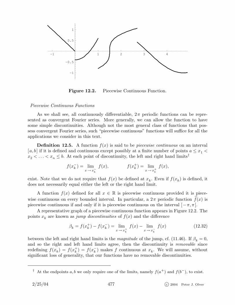
Figure 12.2. Piecewise Continuous Function.
Piecewise Continuous Functions
As we shall see, all continuously differentiable, 2π periodic functions can be repre-sented as convergent Fourier series. More generally, we can allow the function to havesome simple discontinuities. Although not the most general class of functions that pos-sess convergent Fourier series, such “piecewise continuous” functions will suffice for all theapplications we consider in this text.
Definition 12.5. A function f(x) is said to be piecewise continuous on an interval[a, b ] if it is defined and continuous except possibly at a finite number of points a ≤ x1 <x2 < . . . < xn ≤ b. At each point of discontinuity, the left and right hand limits†
f(x−k ) = limx→ x−
k
f(x), f(x+k ) = lim
x→ x+
k
f(x),
exist. Note that we do not require that f(x) be defined at xk. Even if f(xk) is defined, itdoes not necessarily equal either the left or the right hand limit.
A function f(x) defined for all x ∈ R is piecewise continuous provided it is piece-
wise continuous on every bounded interval. In particular, a 2π periodic function f(x) ispiecewise continuous if and only if it is piecewise continuous on the interval [−π, π ].
A representative graph of a piecewise continuous function appears in Figure 12.2. Thepoints xk are known as jump discontinuities of f(x) and the difference
βk = f(x+k )− f(x−k ) = lim
x→ x+
k
f(x)− limx→ x−
k
f(x) (12.32)
between the left and right hand limits is the magnitude of the jump, cf. (11.46). If βk = 0,and so the right and left hand limits agree, then the discontinuity is removable sinceredefining f(xk) = f(x+
k ) = f(x−k ) makes f continuous at xk. We will assume, withoutsignificant loss of generality, that our functions have no removable discontinuities.
† At the endpoints a, b we only require one of the limits, namely f(a+) and f(b−), to exist.
2/25/04 477 c© 2004 Peter J. Olver
-1 1 2 3 4
-1
-0.5
0.5
1
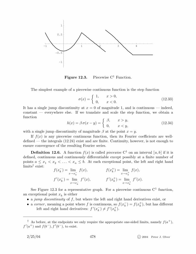
Figure 12.3. Piecewise C1 Function.
The simplest example of a piecewise continuous function is the step function
σ(x) =
{1, x > 0,
0, x < 0.(12.33)
It has a single jump discontinuity at x = 0 of magnitude 1, and is continuous — indeed,constant — everywhere else. If we translate and scale the step function, we obtain afunction
h(x) = β σ(x− y) =
{β, x > y,
0, x < y,(12.34)
with a single jump discontinuity of magnitude β at the point x = y.
If f(x) is any piecewise continuous function, then its Fourier coefficients are well-defined — the integrals (12.24) exist and are finite. Continuity, however, is not enough toensure convergence of the resulting Fourier series.
Definition 12.6. A function f(x) is called piecewise C1 on an interval [a, b ] if it isdefined, continuous and continuously differentiable except possibly at a finite number ofpoints a ≤ x1 < x2 < . . . < xn ≤ b. At each exceptional point, the left and right handlimits† exist:
f(x−k ) = limx→x−
k
f(x), f(x+k ) = lim
x→x+
k
f(x),
f ′(x−k ) = limx→x−
k
f ′(x), f ′(x+k ) = lim
x→x+
k
f ′(x).
See Figure 12.3 for a representative graph. For a piecewise continuous C1 function,an exceptional point xk is either
• a jump discontinuity of f , but where the left and right hand derivatives exist, or• a corner , meaning a point where f is continuous, so f(x−k ) = f(x+
k ), but has differentleft and right hand derivatives: f ′(x−k ) 6= f ′(x+
k ).
† As before, at the endpoints we only require the appropriate one-sided limits, namely f(a+),
f ′(a+) and f(b−), f ′(b−), to exist.
2/25/04 478 c© 2004 Peter J. Olver
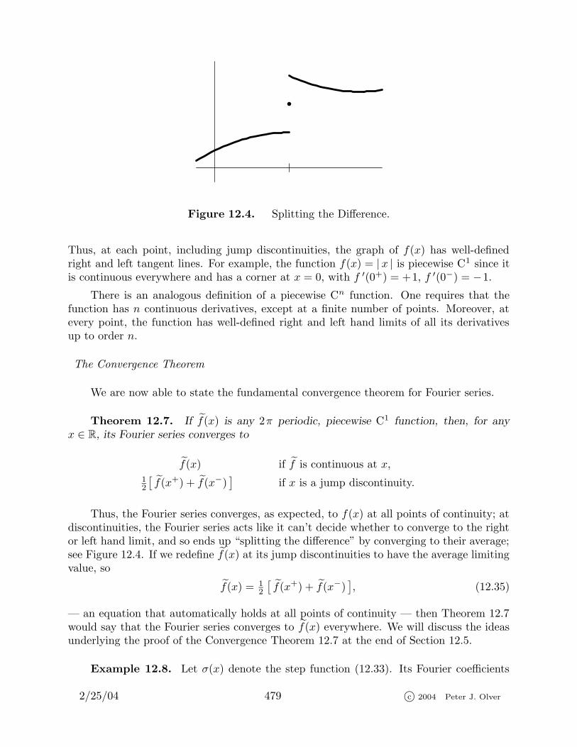
Figure 12.4. Splitting the Difference.
Thus, at each point, including jump discontinuities, the graph of f(x) has well-definedright and left tangent lines. For example, the function f(x) = |x | is piecewise C1 since itis continuous everywhere and has a corner at x = 0, with f ′(0+) = +1, f ′(0−) = −1.
There is an analogous definition of a piecewise Cn function. One requires that thefunction has n continuous derivatives, except at a finite number of points. Moreover, atevery point, the function has well-defined right and left hand limits of all its derivativesup to order n.
The Convergence Theorem
We are now able to state the fundamental convergence theorem for Fourier series.
Theorem 12.7. If f(x) is any 2π periodic, piecewise C1 function, then, for any
x ∈ R, its Fourier series converges to
f(x) if f is continuous at x,12
[f(x+) + f(x−)
]if x is a jump discontinuity.
Thus, the Fourier series converges, as expected, to f(x) at all points of continuity; atdiscontinuities, the Fourier series acts like it can’t decide whether to converge to the rightor left hand limit, and so ends up “splitting the difference” by converging to their average;see Figure 12.4. If we redefine f(x) at its jump discontinuities to have the average limitingvalue, so
f(x) = 12
[f(x+) + f(x−)
], (12.35)
— an equation that automatically holds at all points of continuity — then Theorem 12.7would say that the Fourier series converges to f(x) everywhere. We will discuss the ideasunderlying the proof of the Convergence Theorem 12.7 at the end of Section 12.5.
Example 12.8. Let σ(x) denote the step function (12.33). Its Fourier coefficients
2/25/04 479 c© 2004 Peter J. Olver
-5 5 10 15
-1
-0.5
0.5
1
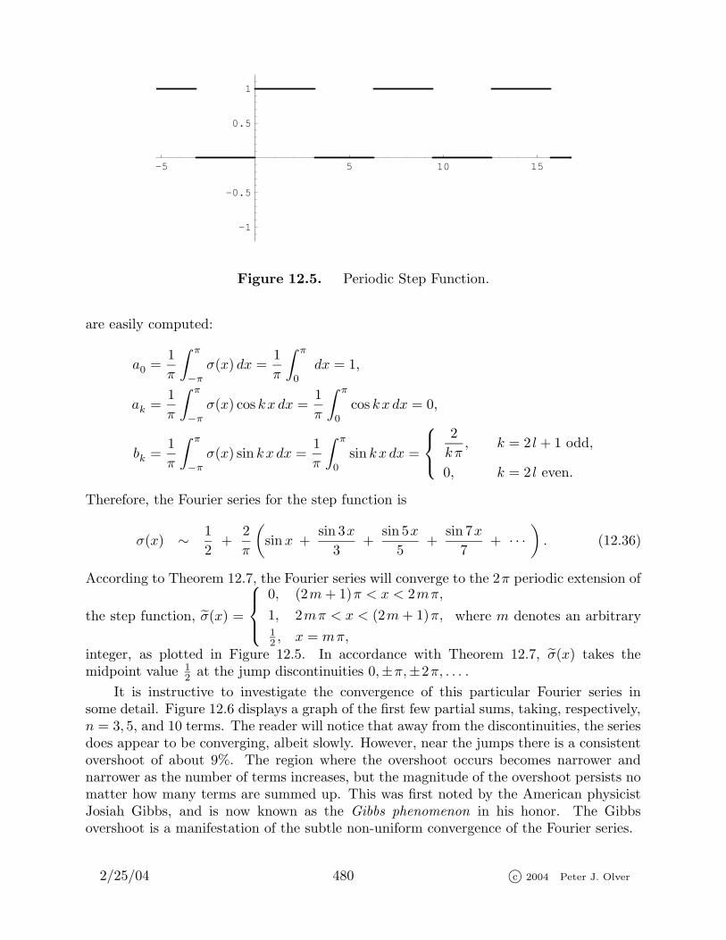
Figure 12.5. Periodic Step Function.
are easily computed:
a0 =1
π
∫ π
−πσ(x) dx =
1
π
∫ π
0
dx = 1,
ak =1
π
∫ π
−πσ(x) cos kx dx =
1
π
∫ π
0
cos kx dx = 0,
bk =1
π
∫ π
−πσ(x) sin kx dx =
1
π
∫ π
0
sin kx dx =
2
kπ, k = 2 l + 1 odd,
0, k = 2 l even.
Therefore, the Fourier series for the step function is
σ(x) ∼ 1
2+2
π
(sinx +
sin 3x
3+sin 5x
5+sin 7x
7+ · · ·
). (12.36)
According to Theorem 12.7, the Fourier series will converge to the 2π periodic extension of
the step function, σ(x) =
0, (2m+ 1)π < x < 2mπ,
1, 2mπ < x < (2m+ 1)π,12 , x = mπ,
where m denotes an arbitrary
integer, as plotted in Figure 12.5. In accordance with Theorem 12.7, σ(x) takes themidpoint value 1
2 at the jump discontinuities 0,±π,±2π, . . . .It is instructive to investigate the convergence of this particular Fourier series in
some detail. Figure 12.6 displays a graph of the first few partial sums, taking, respectively,n = 3, 5, and 10 terms. The reader will notice that away from the discontinuities, the seriesdoes appear to be converging, albeit slowly. However, near the jumps there is a consistentovershoot of about 9%. The region where the overshoot occurs becomes narrower andnarrower as the number of terms increases, but the magnitude of the overshoot persists nomatter how many terms are summed up. This was first noted by the American physicistJosiah Gibbs, and is now known as the Gibbs phenomenon in his honor. The Gibbsovershoot is a manifestation of the subtle non-uniform convergence of the Fourier series.
2/25/04 480 c© 2004 Peter J. Olver
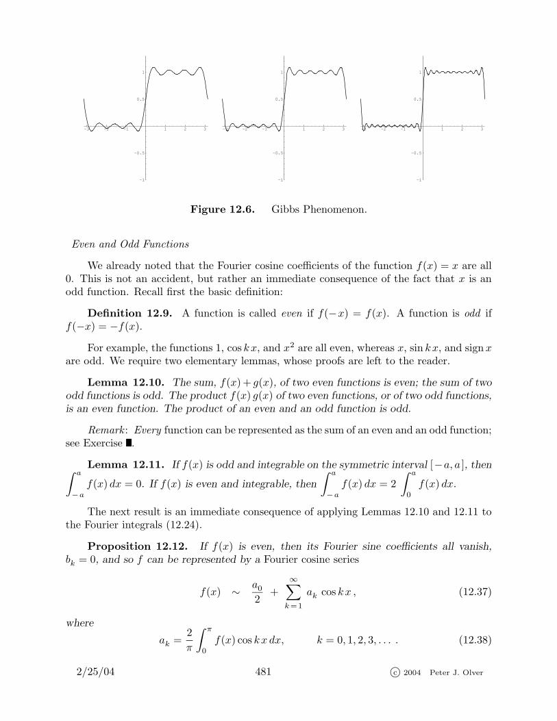
-3 -2 -1 1 2 3
-1
-0.5
0.5
1
-3 -2 -1 1 2 3
-1
-0.5
0.5
1
-3 -2 -1 1 2 3
-1
-0.5
0.5
1
Figure 12.6. Gibbs Phenomenon.
Even and Odd Functions
We already noted that the Fourier cosine coefficients of the function f(x) = x are all0. This is not an accident, but rather an immediate consequence of the fact that x is anodd function. Recall first the basic definition:
Definition 12.9. A function is called even if f(−x) = f(x). A function is odd iff(−x) = −f(x).
For example, the functions 1, cos kx, and x2 are all even, whereas x, sin kx, and signxare odd. We require two elementary lemmas, whose proofs are left to the reader.
Lemma 12.10. The sum, f(x)+ g(x), of two even functions is even; the sum of twoodd functions is odd. The product f(x) g(x) of two even functions, or of two odd functions,is an even function. The product of an even and an odd function is odd.
Remark : Every function can be represented as the sum of an even and an odd function;see Exercise .
Lemma 12.11. If f(x) is odd and integrable on the symmetric interval [−a, a ], then∫ a
−a
f(x) dx = 0. If f(x) is even and integrable, then
∫ a
−a
f(x) dx = 2
∫ a
0
f(x) dx.
The next result is an immediate consequence of applying Lemmas 12.10 and 12.11 tothe Fourier integrals (12.24).
Proposition 12.12. If f(x) is even, then its Fourier sine coefficients all vanish,bk = 0, and so f can be represented by a Fourier cosine series
f(x) ∼ a0
2+
∞∑
k=1
ak cos kx , (12.37)
where
ak =2
π
∫ π
0
f(x) cos kx dx, k = 0, 1, 2, 3, . . . . (12.38)
2/25/04 481 c© 2004 Peter J. Olver

-5 5 10 15
-3
-2
-1
1
2
3
Figure 12.7. Periodic extension of |x |.
If f(x) is odd, then its Fourier cosine coefficients vanish, ak = 0, and so f can be representedby a Fourier sine series
f(x) ∼∞∑
k=1
bk sin kx , (12.39)
where
bk =2
π
∫ π
0
f(x) sin kx dx, k = 1, 2, 3, . . . . (12.40)
Conversely, a convergent Fourier cosine (respectively, sine) series always represents an even(respectively, odd) function.
Example 12.13. The absolute value f(x) = |x | is an even function, and hence hasa Fourier cosine series. The coefficients are
a0 =2
π
∫ π
0
x dx = π, (12.41)
ak =2
π
∫ π
0
x cos kx dx =2
π
[x sin kx
k+cos kx
k2
]π
x=0
=
0, 0 6= k even,
− 4
k2π, k odd.
Therefore
|x | ∼ π
2− 4
π
(cosx +
cos 3x
9+cos 5x
25+cos 7x
49+ · · ·
). (12.42)
According to Theorem 12.7, this Fourier cosine series converges to the 2π periodic extensionof |x |, the “sawtooth function” graphed in Figure 12.7.
In particular, if we substitute x = 0, we obtain another interesting series
π2
8= 1 +
1
9+1
25+1
49+ · · · =
∞∑
n=0
1
(2n+ 1)2. (12.43)
2/25/04 482 c© 2004 Peter J. Olver
It converges faster than Gregory’s series (12.31), and, while far from optimal in this regards,can be used to compute reasonable approximations to π. One can further manipulate thisresult to compute the sum of the series
S =
∞∑
n=1
1
n2= 1 +
1
4+1
9+1
16+1
25+1
36+1
49+ · · · .
We note that
S
4=
∞∑
n=1
1
4n2=
∞∑
n=1
1
(2n)2=1
4+1
16+1
36+1
64+ · · · .
Therefore, by (12.43),
3
4S = S − S
4= 1 +
1
9+1
25+1
49+ · · · = π2
8,
from which we conclude that
S =∞∑
n=1
1
n2= 1 +
1
4+1
9+1
16+1
25+ · · · = π2
6. (12.44)
Remark : The most famous function in number theory — and the source of the mostoutstanding problem in mathematics, the Riemann hypothesis — is the Riemann zetafunction
ζ(s) =∞∑
n=1
1
ns. (12.45)
Formula (12.44) shows that ζ(2) = 16 π
2. In fact, the value of the zeta function at any evenpositive integer s = 2n can be written as a rational polynomial in π.
Remark : If f(x) is either even or odd and 2π periodic, then it is uniquely determinedby its values on the interval [0, π ]. This is proved by a straightforward adaptation of theproof of Lemma 12.3; see Exercise .
Complex Fourier Series
An alternative, and often more convenient, approach to Fourier series is to use complexexponentials instead of sines and cosines. Indeed, Euler’s formula
e i kx = cos kx+ i sin kx, e− i kx = cos kx− i sin kx, (12.46)
shows how to write the trigonometric functions
cos kx =e i kx + e− i kx
2, sin kx =
e i kx − e− i kx
2 i, (12.47)
in terms of complex exponentials. Orthonormality with respect to the rescaled L2 Hermi-tian inner product
〈 f ; g 〉 = 1
2π
∫ π
−πf(x) g(x) dx , (12.48)
2/25/04 483 c© 2004 Peter J. Olver
was proved by direct computation in Example 3.46:
〈 e i kx ; e i lx 〉 = 1
2π
∫ π
−πe i (k−l)x dx =
{1, k = l,
0, k 6= l,
‖ e i kx ‖2 = 1
2π
∫ π
−π| e i kx |2 dx = 1.
(12.49)
Again, orthogonality follows from their status as (complex) eigenfunctions for the periodicboundary value problem (12.9).
The complex Fourier series for a (piecewise continuous) real or complex function f is
f(x) ∼∞∑
k=−∞ck e
i kx = · · · +c−2 e−2 i x+c−1 e
− i x+c0+c1 ei x+c2 e
2 i x+ · · · . (12.50)
The orthonormality formulae (12.48) imply that the complex Fourier coefficients are ob-tained by taking the inner products
ck = 〈 f ; e i kx 〉 = 1
2π
∫ π
−πf(x) e− i kx dx (12.51)
with the associated complex exponential. Pay attention to the minus sign in the integratedexponential — the result of taking the complex conjugate of the second argument in theinner product (12.48). It should be emphasized that the real (12.21) and complex (12.50)Fourier formulae are just two different ways of writing the same series! Indeed, if we applyEuler’s formula (12.46) to (12.51) and compare with the real Fourier formulae (12.24), wefind that the real and complex Fourier coefficients are related by
ak = ck + c−k,
bk = i (ck − c−k),
ck =12 (ak − i bk),
c−k =12 (ak + i bk),
k = 0, 1, 2, . . . . (12.52)
Remark : We already see one advantage of the complex version. The constant function1 = e0 i x no longer plays an anomalous role — the annoying factor of 1
2 in the real Fourierseries (12.21) has mysteriously disappeared!
Example 12.14. For the step function σ(x) considered in Example 12.8, the complexFourier coefficients are
ck =1
2π
∫ π
−πσ(x) e− i kx dx =
1
2π
∫ π
0
e− i kx dx =
12 , k = 0,
0, 0 6= k even,
1
i k π, k odd.
Therefore, the step function has the complex Fourier series
σ(x) ∼ 1
2− i
π
∞∑
l=−∞
e(2 l+1) i x
2 l + 1.
2/25/04 484 c© 2004 Peter J. Olver

You should convince yourself that this is exactly the same series as the real Fourier series(12.36). We are merely rewriting it using complex exponentials instead of real sines andcosines.
Example 12.15. Let us find the Fourier series for the exponential function eax. Itis much easier to evaluate the integral for the complex Fourier coefficients, and so
ck = 〈 eax ; e i kx 〉 = 1
2π
∫ π
−πe(a− i k)x dx =
e(a− i k)x
2π (a− i k)
∣∣∣∣π
x=−π
=e(a− i k)π − e−(a− i k)π
2π (a− i k) = (−1)k eaπ − e−aπ
2π (a− i k) =(−1)k(a+ i k) sinh aπ
π (a2 + k2).
Therefore, the desired Fourier series is
eax ∼ sinh aπ
π
∞∑
k=−∞
(−1)k(a+ i k)a2 + k2
e i kx. (12.53)
As an exercise, the reader should try writing this as a real Fourier series, either by breakingup the complex series into its real and imaginary parts, or by direct evaluation of the realcoefficients via their integral formulae (12.24).
The Delta Function
Fourier series can even be used to represent more general objects than mere functions.The most important example is the delta function δ(x). Using its characterizing properties(11.37), the real Fourier coefficients are computed as
ak =1
π
∫ π
−πδ(x) cos kx dx =
1
πcos k0 =
1
π,
bk =1
π
∫ π
−πδ(x) sin kx dx =
1
πsin k0 = 0.
(12.54)
Therefore,
δ(x) ∼ 1
2π+1
π
(cosx+ cos 2x+ cos 3x+ · · ·
). (12.55)
Since δ(x) is an even function, it should come as no surprise that it has a cosine series.
To understand in what sense this series converges to the delta function, it will help torewrite it in complex form
δ(x) ∼ 1
2π
∞∑
k=−∞e i kx =
1
2π
(· · · + e−2 i x + e− i x + 1 + e i x + e2 i x + · · ·
). (12.56)
where the complex Fourier coefficients are computed† as
ck =1
2π
∫ π
−πδ(x) e− i kx dx =
1
2π.
† Or, we could use (12.52).
2/25/04 485 c© 2004 Peter J. Olver
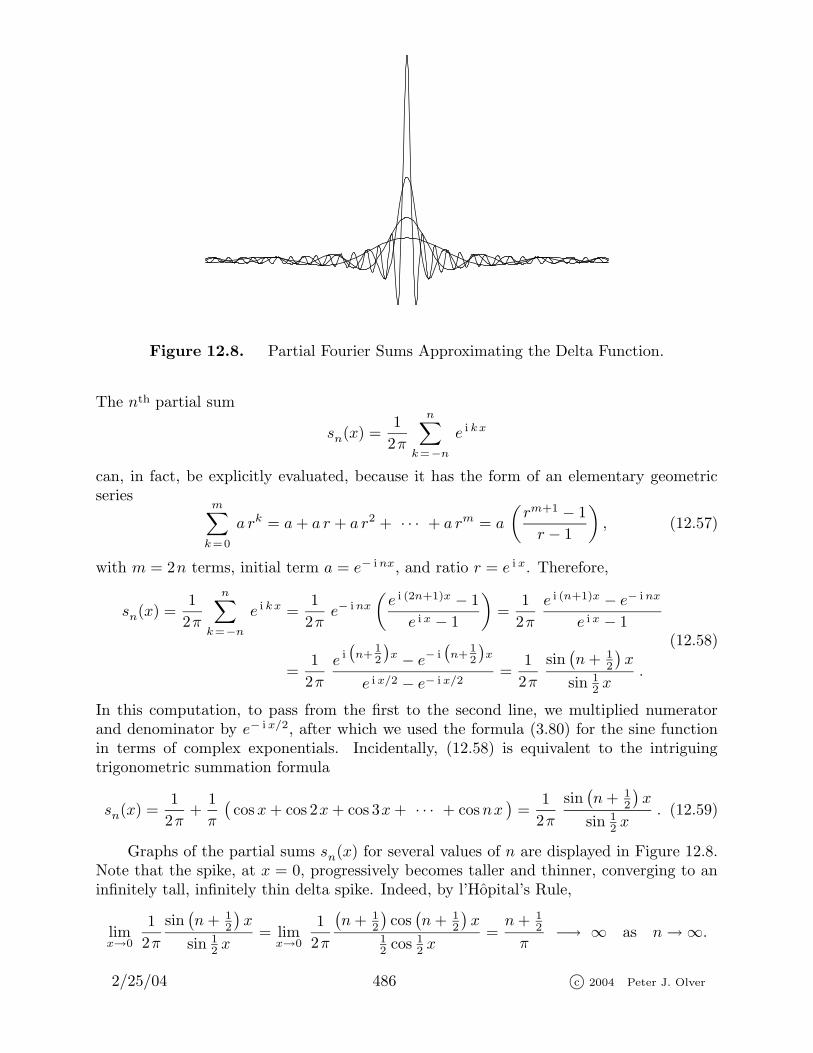
Figure 12.8. Partial Fourier Sums Approximating the Delta Function.
The nth partial sum
sn(x) =1
2π
n∑
k=−ne i kx
can, in fact, be explicitly evaluated, because it has the form of an elementary geometricseries
m∑
k=0
a rk = a+ a r + a r2 + · · · + a rm = a
(rm+1 − 1r − 1
), (12.57)
with m = 2n terms, initial term a = e− inx, and ratio r = e i x. Therefore,
sn(x) =1
2π
n∑
k=−ne i kx =
1
2πe− inx
(e i (2n+1)x − 1
e i x − 1
)=1
2π
e i (n+1)x − e− inx
e i x − 1
=1
2π
e i(n+
12
)x − e− i
(n+
12
)x
e i x/2 − e− i x/2=1
2π
sin(n+ 1
2
)x
sin 12 x
.
(12.58)
In this computation, to pass from the first to the second line, we multiplied numeratorand denominator by e− i x/2, after which we used the formula (3.80) for the sine functionin terms of complex exponentials. Incidentally, (12.58) is equivalent to the intriguingtrigonometric summation formula
sn(x) =1
2π+1
π
(cosx+ cos 2x+ cos 3x+ · · · + cosnx
)=1
2π
sin(n+ 1
2
)x
sin 12 x
. (12.59)
Graphs of the partial sums sn(x) for several values of n are displayed in Figure 12.8.Note that the spike, at x = 0, progressively becomes taller and thinner, converging to aninfinitely tall, infinitely thin delta spike. Indeed, by l’Hopital’s Rule,
limx→0
1
2π
sin(n+ 1
2
)x
sin 12 x
= limx→0
1
2π
(n+ 1
2
)cos(n+ 1
2
)x
12 cos
12 x
=n+ 1
2
π−→ ∞ as n→∞.
2/25/04 486 c© 2004 Peter J. Olver

(An elementary proof of this fact is to note that, at x = 0, every term in the original sum(12.56) is equal to 1.) Furthermore, the integrals remain fixed
1
2π
∫ π
−πsn(x) dx =
1
2π
∫ π
−π
sin(n+ 1
2
)x
sin 12 x
dx =1
2π
∫ π
−π
n∑
k=−ne i kx dx = 1, (12.60)
as required for convergence to the delta function. However, away from the spike, the par-tial sums do not go to zero! Rather, they oscillate more and more rapidly, maintainingan overall amplitude of 1
2π csc12 x = 1/
(2π sin 1
2 x). As n gets large, the amplitude func-
tion appears as an envelope of the increasingly rapid oscillations. Roughly speaking, thefact that sn(x) → δ(x) as n → ∞ means that the “infinitely fast” oscillations somehowcancel each other out, and the net effect is zero away from the spike at x = 0. Thus,the convergence of the Fourier sums to δ(x) is much more subtle than in the original lim-iting definition (11.32). The technical term is “weak convergence”, which plays an veryimportant role in advanced mathematical analysis, [126].
Remark : Although we stated that the Fourier series (12.55), (12.56) represent thedelta function, this is not entirely correct. Remember that a Fourier series converges tothe 2π periodic extension of the original function. Therefore, (12.56) actually representsthe periodic extension of the delta function
δ(x) = · · · +δ(x+4π)+δ(x+2π)+δ(x)+δ(x−2π)+δ(x−4π)+δ(x−6π)+ · · · , (12.61)
consisting of a periodic array of delta spikes concentrated at all integer multiples of 2π.
12.3. Differentiation and Integration.
If a series of functions converges “nicely” then one expects to be able to integrateand differentiate it term by term; the resulting series should converge to the integral andderivative of the original sum. For power series, this is always valid within the range ofconvergence, and is used extensively in the construction of series solutions of differentialequations, series for integrals of non-elementary functions, and so on. The interested readershould consult Appendix C for the details.
As we now appreciate, the convergence of Fourier series is a much more delicatematter, and so one must take considerably more care in the application of term-wisedifferentiation and integration. Nevertheless, in favorable situations, both operations leadto valid results, and provide useful mechanisms for constructing Fourier series of morecomplicated functions. It is a remarkable, profound fact that Fourier analysis is completelycompatible with the calculus of generalized functions that we developed in Chapter 11.For instance, differentiating the Fourier series for a suitably nice function with a jumpdiscontinuity leads to the Fourier series for the differentiated function, with a delta functionof the appropriate magnitude appearing at the discontinuity. This fact reassures us thatthe rather mysterious construction of delta functions and their generalizations is indeed theright way to extend calculus to functions which do not possess derivatives in the ordinarysense.
2/25/04 487 c© 2004 Peter J. Olver
Integration of Fourier Series
Integration is a smoothing operation — the integrated function is always nicer thanthe original. Therefore, we should anticipate being able to integrate Fourier series withoutdifficulty. There is, however, one complication: the integral of a periodic function is notnecessarily periodic. The simplest example is the constant function 1, which is certainlyperiodic, but its integral, namely x, is not. On the other hand, integrals of all the otherperiodic sine and cosine functions appearing in the Fourier series are periodic. Thus, onlythe constant term might cause us difficulty when we try to integrate a Fourier series (12.21).According to (2.4), the constant term
a0
2=1
2π
∫ π
−πf(x) dx (12.62)
is the mean or average of the function f(x) on the interval [−π, π ]. A function has noconstant term in its Fourier series if and only if it has zero mean. It is easily shown,cf. Exercise , that the mean zero functions are precisely the ones that remain periodicupon integration.
Lemma 12.16. If f(x) is 2π periodic, then its integral g(x) =
∫ x
0
f(y) dy is 2π
periodic if and only if f has mean zero on the interval [−π, π ].
In particular, Lemma 12.11 implies that all odd functions automatically have meanzero, and hence periodic integrals.
Since ∫cos kx dx =
sin kx
k,
∫sin kx dx = − cos kx
k, (12.63)
termwise integration of a Fourier series without constant term is straightforward. Theresulting Fourier series is given precisely as follows.
Theorem 12.17. If f is piecewise continuous, 2π periodic, and has mean zero, thenits Fourier series can be integrated term by term, to produce the Fourier series
g(x) =
∫ x
0
f(y) dy ∼ m +
∞∑
k=1
[− bk
kcos kx+
akksin kx
], (12.64)
for its periodic integral. The constant term
m =1
2π
∫ π
−πg(x) dx
is the mean of the integrated function.
In many situations, the integration formula (12.64) provides a very convenient alter-native to the direct derivation of the Fourier coefficients.
2/25/04 488 c© 2004 Peter J. Olver

Example 12.18. The function f(x) = x is odd, and so has mean zero,
∫ π
−πx dx = 0.
Let us integrate its Fourier series
x ∼ 2∞∑
k=1
(−1)k−1
ksin kx (12.65)
that we found in Example 12.2. The result is the Fourier series
1
2x2 ∼ π2
6− 2
∞∑
k=1
(−1)k−1
k2cos kx
∼ π2
6− 2
(cosx − cos 2x
4+cos 3x
9− cos 4x
16+ · · ·
),
(12.66)
whose the constant term is the mean of the left hand side:
1
2π
∫ π
−π
x2
2dx =
π2
6.
If we were to integrate each trigonometric summand in a Fourier series (12.21) from0 to x, we would obtain
∫ x
0
cos ky dy =sin kx
k, whereas
∫ x
0
sin ky dy =1
k− cos kx
k.
The extra 1/k terms arising from the sine integrals do not appear explicitly our previousform for the integrated Fourier series, (12.64), and so must be hidden in the constant termm. We deduce that the mean value of the integrated function can be computed using theFourier sine coefficients of f via the formula
1
2π
∫ π
−πg(x) dx = m =
∞∑
k=1
bkk. (12.67)
For example, the result of integrating both sides of the Fourier series (12.65) from 0 to xis
x2
2∼ 2
∞∑
k=1
(−1)k−1
k2(1− cos kx).
The constant terms sum up to yield the mean value of the integrated function:
2
(1− 1
4+1
9− 1
16+ . . .
)= 2
∞∑
k=1
(−1)k−1
k2=
1
2π
∫ π
−π
x2
2dx =
π2
6, (12.68)
which reproduces a formula established in Exercise .
More generally, if f(x) does not have mean zero, its Fourier series has a nonzeroconstant term,
f(x) ∼ a0
2+
∞∑
k=1
[ ak cos kx+ bk sin kx ] .
2/25/04 489 c© 2004 Peter J. Olver
In this case, the result of integration will be
g(x) =
∫ x
0
f(y) dy ∼ a0
2x+m+
∞∑
k=1
[− bk
kcos kx+
akksin kx
], (12.69)
where m is given in (12.67). The right hand side is not, strictly speaking, a Fourier series.There are two ways to interpret this formula within the Fourier framework. Either we canwrite (12.69) as the Fourier series for the difference
g(x)− a0
2x ∼ m+
∞∑
k=1
[− bk
kcos kx+
akksin kx
], (12.70)
which is a 2π periodic function, cf. Exercise . Alternatively, one can replace x by itsFourier series (12.26), and the result will be the Fourier series for the 2π periodic extension
of the integral g(x) =
∫ x
0
f(y) dy.
Differentiation of Fourier Series
Differentiation has the opposite effect to integration. Differentiation makes a functionworse. Therefore, to justify taking the derivative of a Fourier series, we need to know thatthe differentiated function remains reasonably nice. Since we need the derivative f ′(x) tobe piecewise C1 for the convergence Theorem 12.7 to be applicable, we have to requirethat f(x) itself be continuous and piecewise C2.
Theorem 12.19. If f is 2π periodic, continuous, and piecewise C2, then its Fourier
series can be differentiated term by term, to produce the Fourier series for its derivative
f ′(x) ∼∞∑
k=1
[k bk cos kx− k ak sin kx
]. (12.71)
Example 12.20. The derivative (11.52) of the absolute value function f(x) = |x |is the sign function
d |x |dx
= signx =
{+1, x > 0
−1, x < 0.
Therefore, if we differentiate its Fourier series (12.42), we obtain the Fourier series
signx ∼ 4
π
(sinx +
sin 3x
3+sin 5x
5+sin 7x
7+ · · ·
). (12.72)
Note that signx = σ(x)−σ(−x) is the difference of two step functions. Indeed, subtractingthe step function Fourier series (12.36) at x from the same series at −x reproduces (12.72).
Example 12.21. If we differentiate the Fourier series
x ∼ 2
∞∑
k=1
(−1)k−1
ksin kx = 2
(sinx − sin 2x
2+sin 3x
3− sin 4x
4+ · · ·
),
2/25/04 490 c© 2004 Peter J. Olver
we obtain an apparent contradiction:
1 ∼ 2
∞∑
k=1
(−1)k+1 cos kx = 2− 2 cosx+ 2 cos 2x− 2 cos 3x+ · · · . (12.73)
But the Fourier series for 1 just consists of a single constant term! (Why?)
The resolution of this paradox is not difficult. The Fourier series (12.26) does not
converge to x, but rather to its periodic extension f(x), which has a jump discontinuityof magnitude 2π at odd multiples of π. Thus, Theorem 12.19 is not directly applicable.Nevertheless, we can assign a consistent interpretation to the differentiated series. Thederivative f ′(x) of the periodic extension is not equal to the constant function 1, but,rather, has an additional delta function concentrated at each jump discontinuity:
f ′(x) = 1− 2π∞∑
j=−∞δ(x− (2j + 1)π
)= 1− 2π δ(x− π),
where δ denotes the 2π periodic extension of the delta function, cf. (12.61). The dif-ferentiated Fourier series (12.73) does, in fact, converge to this modified distributionalderivative! Indeed, differentiation and integration of Fourier series is entirely compatiblewith the calculus of generalized functions, as will be borne out in yet another example.
Example 12.22. Let us differentiate the Fourier series (12.36) for the step functionand see if we end up with the Fourier series (12.55) for the delta function. We find (12.36)
d
dxσ(x) ∼ 2
π
(cosx+ cos 3x+ cos 5x+ cos 7x+ · · ·
), (12.74)
which does not agree with (12.55) — half the terms are missing! the explanation issimilar to the preceding example: the 2π periodic extension of the step function has twojump discontinuities, of magnitudes +1 at even multiples of π and −1 at odd multiples.Therefore, its derivative is the difference of the 2π periodic extension of the delta functionat 0, with Fourier series (12.55) minus the 2π periodic extension of the delta function atπ, with Fourier series
δ(x− π) ∼ 2
π− 1
π
(cosx+ cos 2x+ cos 3x+ · · ·
).
The difference of these two delta function series produces (12.74).
12.4. Change of Scale.
So far, we have only dealt with Fourier series on the standard interval of length 2π.(We chose [−π, π ] for convenience, but all of the results and formulas are easily adaptedto any other interval of the same length, e.g., [0, 2π ].) Since physical objects like bars andstrings do not all come in this particular length, we need to understand how to adapt theformulas to more general intervals. The basic idea is to rescale the variable so as to stretchor contract the standard interval. This device was already used, in Section 5.4, to adaptthe orthogonal Legendre polynomials to other intervals.
2/25/04 491 c© 2004 Peter J. Olver
Any symmetric interval [−` , ` ] of length 2 ` can be rescaled to the standard interval[−π, π ] by using the linear change of variables
x =`
πy, so that − π ≤ y ≤ π whenever − ` ≤ x ≤ `. (12.75)
Given a function f(x) defined on [−` , ` ], the rescaled function F (y) = f
(`
πy
)lives on
[−π, π ]. Let
F (y) ∼ a0
2+
∞∑
k=1
[ak cos ky + bk sin ky
],
be the standard Fourier series for F (y), so that
ak =1
π
∫ π
−πF (y) cos ky dy, bk =
1
π
∫ π
−πF (y) sin ky dy. (12.76)
Then, reverting to the unscaled variable x, we deduce that
f(x) ∼ a0
2+
∞∑
k=1
[ak cos
kπx
`+ bk sin
kπx
`
]. (12.77)
The Fourier coefficients ak, bk can be computed directly from f(x). Indeed, replacing theintegration variable by y = πx/`, and noting that dy = (π/`) dx, we deduce the adaptedformulae
ak =1
`
∫ `
−`f(x) cos
kπx
`dx, bk =
1
`
∫ `
−`f(x) sin
kπx
`dx, (12.78)
for the Fourier coefficients of f(x) on the interval [−` , ` ].All of the convergence results, integration and differentiation formulae, etc., that
are valid for the interval [−π, π ] carry over, essentially unchanged, to Fourier series onnonstandard intervals. In particular, adapting our basic convergence Theorem 12.7, weconclude that if f(x) is piecewise C1, then its rescaled Fourier series (12.77) converges
to its 2 ` periodic extension f(x), subject to the proviso that f(x) takes on the midpointvalues at all jump discontinuities.
Example 12.23. Let us compute the Fourier series for the function f(x) = x on theinterval −1 ≤ x ≤ 1. Since f is odd, only the sine coefficients will be nonzero. We have
bk =
∫ 1
−1
x sin kπx dx =
[− x cos kπx
kπ+sin kπx
(kπ)2
]1
x=−1
=2(−1)k+1
k π.
The resulting Fourier series is
x ∼ 2
π
(sinπx − sin 2πx
2+sin 3πx
3− · · ·
).
2/25/04 492 c© 2004 Peter J. Olver
The series converges to the 2 periodic extension of the function x, namely
f(x) =
{x− 2m, 2m− 1 < x < 2m+ 1,
0, x = m,where m is an arbitrary integer.
We can similarly reformulate complex Fourier series on the nonstandard interval[−` , ` ]. Scaling the variables in (12.50) in (12.75), we find
f(x) ∼∞∑
k=−∞ck e
i kπx/`, where ck =1
2 `
∫ `
−`f(x) e− i kπx/` dx. (12.79)
Again, this is merely an alternative way of writing the real Fourier series (12.77).
For a more general interval [a, b ] there are two options. The first is to take a function
f(x) defined for a ≤ x ≤ b and periodically extend it to a function f(x) that agrees withf(x) on [a, b ] and has period b − a. One can then compute the Fourier series (12.77) forthe periodic extension on the symmetric interval [ 12 (a− b), 1
2 (b− a) ] of width 2 ` = b− a;the resulting Fourier series will (under the appropriate hypotheses) converge to f(x) andhence agree with f(x) on the original interval. An alternative approach is to translate theinterval by an amount 1
2 (a + b) so as to make it symmetric; this is accomplished by thechange of variables x = x− 1
2 (a+ b). an additional rescaling will convert the interval into[−π, π ]. The two methods are essentially equivalent, and full details are left to the reader.
12.5. Convergence of the Fourier Series.
The purpose of this final section is to establish some basic convergence results forFourier series. As a by product, we obtain additional information about the nature ofFourier series that plays an important role in applications, particularly the interplay be-tween the smoothness of the function and the decay of its Fourier coefficients, a result thatis exploited in signal and image denoising and in the analytical properties of solutions topartial differential equations. Be forewarned: the material will be more theoretical thanwe are used to, and the more applied reader may consider omitting it on a first reading.However, a full understanding of the range of Fourier analysis does requires some familiar-ity with the underlying theoretical developments. Moreover, the required techniques andproofs serve as an excellent introduction to some of the most important tools of modernmathematical analysis. The effort expended to assimilate this material will be more thanamply rewarded in your later career.
Unlike power series, which converge to analytic functions on the interval of conver-gence, and diverge elsewhere (the only tricky point being whether or not the series con-verges at the endpoints), the convergence of a Fourier series is a much more subtle matter,and still not understood in complete generality. A large part of the difficulty stems fromthe intricacies of convergence in infinite-dimensional function spaces. Let us thereforebegin with a brief discussion of the fundamental issues.
Convergence in Vector Spaces
We assume that you are familiar with the usual calculus definition of the limit ofa sequence of real numbers: lim
n→∞a(n) = a?. In a finite-dimensional vector space, e.g.,
2/25/04 493 c© 2004 Peter J. Olver
Rm, convergence of sequences is straightforward. There is essentially only one way for asequence of vectors v(0),v(1),v(2), . . . ∈ R
m to converge, as guaranteed by any one of thefollowing equivalent criteria:
(a) The vectors converge: v(n) −→ v? ∈ Rm as n→∞.
(b) All components of v(n) = (v(n)1 , . . . , v(n)
m ) converge, so v(n)i −→ v?i , for i = 1, . . . ,m.
(c) The difference in norms goes to zero: ‖v(n) − v? ‖ −→ 0 as n→∞.The last requirement, known as convergence in norm, does not, in fact, depend on whichnorm is chosen. Indeed, Theorem 3.19 implies that, on a finite-dimensional vector space,all norms are essentially equivalent, and if one norm goes to zero, so does any other norm.
The corresponding convergence criteria are certainly not the same in infinite-dim-ensional vector spaces. There are, in fact, a bewildering variety of diverse convergencemechanisms in function space, including pointwise convergence, uniform convergence, con-vergence in norm, weak convergence, and so on. All play a significant role in advancedmathematical analysis. But, for our purposes, we shall be content to study just the mostbasic aspects of convergence of the Fourier series. Much more detail is available in moreadvanced texts, e.g., [51, 159].
The most basic convergence mechanism for a sequence of functions vn(x) is calledpointwise convergence, where we require
limn→∞
vn(x) = v?(x) for all x. (12.80)
In other words, the functions’ values at each individual point converge in the usual sense.Pointwise convergence is the function space version of the convergence of the components ofa vector. Indeed, pointwise convergence immediately implies component-wise convergenceof the sample vectors v(n) = ( vn(x1), . . . , vn(xm) )
T ∈ Rm for any choice of sample points.
On the other hand, convergence in norm of the function sequence requires
limn→∞
‖ vn − v? ‖ = 0,
where ‖ · ‖ is a prescribed norm on the function space. As we have learned, not all normson an infinite-dimensional function space are equivalent: a function might be small in onenorm, but large in another. As a result, convergence in norm will depend upon the choiceof norm. Moreover, convergence in norm does not necessarily imply pointwise convergenceor vice versa. A variety of examples can be found in the exercises.
Uniform Convergence
Proving uniform convergence of a Fourier series is reasonably straightforward, andso we will begin there. You no doubt first saw the concept of a uniformly convergentsequence of functions in your calculus course, although chances are it didn’t leave muchof an impression. In Fourier analysis, uniform convergence begins to play an increasinglyimportant role, and is worth studying in earnest. For the record, let us restate the basicdefinition.
2/25/04 494 c© 2004 Peter J. Olver
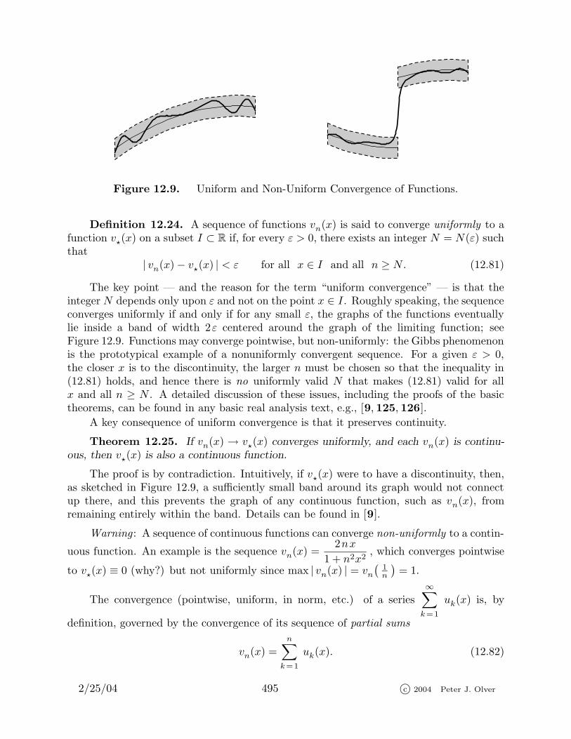
Figure 12.9. Uniform and Non-Uniform Convergence of Functions.
Definition 12.24. A sequence of functions vn(x) is said to converge uniformly to afunction v?(x) on a subset I ⊂ R if, for every ε > 0, there exists an integer N = N(ε) suchthat
| vn(x)− v?(x) | < ε for all x ∈ I and all n ≥ N . (12.81)
The key point — and the reason for the term “uniform convergence” — is that theinteger N depends only upon ε and not on the point x ∈ I. Roughly speaking, the sequenceconverges uniformly if and only if for any small ε, the graphs of the functions eventuallylie inside a band of width 2ε centered around the graph of the limiting function; seeFigure 12.9. Functions may converge pointwise, but non-uniformly: the Gibbs phenomenonis the prototypical example of a nonuniformly convergent sequence. For a given ε > 0,the closer x is to the discontinuity, the larger n must be chosen so that the inequality in(12.81) holds, and hence there is no uniformly valid N that makes (12.81) valid for allx and all n ≥ N . A detailed discussion of these issues, including the proofs of the basictheorems, can be found in any basic real analysis text, e.g., [9, 125, 126].
A key consequence of uniform convergence is that it preserves continuity.
Theorem 12.25. If vn(x) → v?(x) converges uniformly, and each vn(x) is continu-ous, then v?(x) is also a continuous function.
The proof is by contradiction. Intuitively, if v?(x) were to have a discontinuity, then,as sketched in Figure 12.9, a sufficiently small band around its graph would not connectup there, and this prevents the graph of any continuous function, such as vn(x), fromremaining entirely within the band. Details can be found in [9].
Warning : A sequence of continuous functions can converge non-uniformly to a contin-
uous function. An example is the sequence vn(x) =2nx
1 + n2x2, which converges pointwise
to v?(x) ≡ 0 (why?) but not uniformly since max | vn(x) | = vn(
1n
)= 1.
The convergence (pointwise, uniform, in norm, etc.) of a series∞∑
k=1
uk(x) is, by
definition, governed by the convergence of its sequence of partial sums
vn(x) =
n∑
k=1
uk(x). (12.82)
2/25/04 495 c© 2004 Peter J. Olver

The most useful test for uniform convergence of series of functions is known as the Weier-strass M–test , due to the highly influential nineteenth century German mathematicianKarl Weierstrass, the “father of modern analysis”.
Theorem 12.26. Suppose the functions uk(x) are bounded by
|uk(x) | ≤ mk for all x ∈ I, (12.83)
where the mk ≥ 0 are fixed positive constants. If the series∞∑
k=1
mk <∞ (12.84)
converges, then the series∞∑
k=1
uk(x) = f(x) (12.85)
converges uniformly to a function f(x) for all x ∈ I. In particular, if the summands uk(x)in Theorem 12.26 are continuous, so is the sum f(x).
With some care, we are allowed to manipulate uniformly convergent series just likefinite sums. Thus, if (12.85) is a uniformly convergent series, so is the term-wise product
∞∑
k=1
g(x)uk(x) = g(x)f(x) (12.86)
with any bounded function: | g(x) | ≤ C for x ∈ I. We can integrate a uniformly convergentseries term by term, and the integrated series
∫ x
a
( ∞∑
k=1
uk(y)
)dy =
∞∑
k=1
∫ x
a
uk(y) dy =
∫ x
a
f(y) dy (12.87)
is uniformly convergent. Differentiation is also allowed — but only when the differentiatedseries converges uniformly.
Proposition 12.27. If
∞∑
k=1
u′k(x) = g(x) is a uniformly convergent series, then
∞∑
k=1
uk(x) = f(x) is also uniformly convergent, and, moreover, f ′(x) = g(x).
We are particularly interested in applying these results to Fourier series, which, forconvenience, we take in complex form
f(x) ∼∞∑
k=−∞ck e
i kx. (12.88)
2/25/04 496 c© 2004 Peter J. Olver
Since x is real,∣∣ e i kx
∣∣ ≤ 1, and hence the individual summands are bounded by∣∣ ck e i kx
∣∣ ≤ | ck | for all x.
Applying the Weierstrass M–test, we immediately deduce the basic result on uniformconvergence of Fourier series.
Theorem 12.28. If the Fourier coefficients ck satisfy
∞∑
k=−∞| ck | <∞, (12.89)
then the Fourier series (12.88) converges uniformly to a continuous function f(x) havingthe same Fourier coefficients ck.
Proof : Uniform convergence and continuity of the limiting function follow from Theo-rem 12.26. To show that the ck actually are the Fourier coefficients of the sum, we multiplythe Fourier series by e− i kx and integrate term by term from−π to π. As in (12.86), (12.87),both operations are valid thanks to the uniform convergence of the series. Q.E.D.
The one thing that the theorem does not guarantee is that the original function f(x)
used to compute the Fourier coefficients ck is the same as the function f(x) obtained bysumming the resulting Fourier series! Indeed, this may very well not be the case. As weknow, the function that the series converges to is necessarily 2π periodic. Thus, at thevery least, f(x) will be the 2π periodic extension of f(x). But even this may not suffice.
Two functions f(x) and f(x) that have the same values except for a finite set of pointsx1, . . . , xm have the same Fourier coefficients. (Why?) More generally, two functions whichagree everywhere outside a set of “measure zero” will have the same Fourier coefficients.In this way, a convergent Fourier series singles out a distinguished representative from acollection of essentially equivalent 2π periodic functions.
Remark : The term “measure” refers to a rigorous generalization of the notion of thelength of an interval to more general subsets S ⊂ R. In particular, S has measure zeroif it can be covered by a collection of intervals of arbitrarily small total length. Forexample, any collection of finitely many points, or even countably many points, e.g., therational numbers, has measure zero. The proper development of the notion of measure,and the consequential Lebesgue theory of integration, is properly studied in a course inreal analysis, [125, 126].
Fourier series cannot converge uniformly when discontinuities are present. However, itcan be proved, [28, 51, 159], that even when the function fails to be everywhere continuous,its Fourier series is uniformly convergent on any closed subset of continuity.
Theorem 12.29. Let f(x) be 2π periodic and piecewise C1. If f is continuous fora < x < b, then its Fourier series converges uniformly to f(x) on any closed subintervala+ δ ≤ x ≤ b− δ, with δ > 0.
2/25/04 497 c© 2004 Peter J. Olver
For example, the Fourier series (12.36) for the step function does converge uniformlyif we stay away from the discontinuities; for instance, by restriction to a subinterval ofthe form [δ, π − δ ] or [−π + δ,−δ ] for any 0 < δ < 1
2 π. This reconfirms our observationthat the nonuniform Gibbs behavior becomes progressively more and more localized at thediscontinuities.
Smoothness and Decay
The uniform convergence criterion (12.89) requires, at the very least, that the Fouriercoefficients decay to zero: ck → 0 as k → ±∞. In fact, the Fourier coefficients cannottend to zero too slowly. For example, the individual summands of the infinite series
∞∑
k=−∞
1
| k |α (12.90)
go to 0 as k →∞ whenever α > 0, but the series only converges when α > 1. (This followsfrom the standard integral test for series, [9, 126].) Thus, if we can bound the Fouriercoefficients by
| ck | ≤M
| k |α for all | k | À 0, (12.91)
for some power α > 1 and some positive constant M > 0, then the Weierstrass M test willguarantee that the Fourier series converges uniformly to a continuous function.
An important consequence of the differentiation formulae (12.71) for Fourier series isthe fact that the faster the Fourier coefficients of a function tend to zero as k → ∞, thesmoother the function is. Thus, one can detect the degree of smoothness of a function byhow rapidly its Fourier coefficients decay to zero. More rigorously, we have:
Theorem 12.30. If the Fourier coefficients satisfy
∞∑
k=−∞kn | ck | < ∞, (12.92)
then the Fourier series (12.50) converges to a 2π periodic function which is n times con-tinuously differentiable: f(x) ∈ Cn. Moreover, for any m ≤ n, the m times differentiated
Fourier series converges uniformly to the corresponding derivative f (m)(x).
Proof : This is an immediate consequence of Proposition 12.27 and Theorem 12.28.Application of the Weierstrass M test to the differentiated Fourier series based on ourhypothesis (12.92) serves to complete the proof. Q.E.D.
Corollary 12.31. If the Fourier coefficients satisfy (12.91) for some α > n+1, thenthe function f(x) is n times continuously differentiable.
Thus, stated roughly, the smaller the high frequency Fourier coefficients are, thesmoother the function is. If the Fourier coefficients go to zero faster than any powerof k, e.g., exponentially fast, then the function is infinitely differentiable. Analyticity is alittle more delicate, and we refer the reader to [51, 159] for details.
2/25/04 498 c© 2004 Peter J. Olver

Example 12.32. The 2π periodic extension of the function |x | is continuous withpiecewise continuous first derivative. Its Fourier coefficients (12.41) satisfy the estimate(12.91) for α = 2, which is just shy of sufficing for a continuous second derivative. On theother hand, the Fourier coefficients (12.25) of the step function σ(x) only tend to zero as1/k, so α = 1, reflecting the fact that its periodic extension is only piecewise continuous.Finally, the Fourier coefficients (12.54) for the delta function do not tend to zero at all,indicative of the fact that it is not an ordinary function, and its Fourier series does notconverge in the standard sense.
Hilbert Space
In order to make further progress, we must take a little detour. The proper settingfor the rigorous theory of Fourier series turns out to be the most important function spacein modern physics and modern analysis, known as Hilbert space. The precise definition ofthis infinite-dimensional inner product space is rather technical, but a rough version goesas follows:
Definition 12.33. A complex-valued function f(x) is called square-integrable on theinterval [−π, π ] if it satisfies
‖ f ‖2 = 1
2π
∫ π
−π| f(x) |2 dx <∞. (12.93)
The Hilbert space L2 = L2[−π, π ] is the vector space consisting of all complex-valuedsquare-integrable functions.
Note that (12.93) is the L2 norm based on the standard Hermitian inner product
〈 f ; g 〉 = 1
2π
∫ π
−πf(x) g(x) dx. (12.94)
The triangle inequality
‖ c f + d g ‖ ≤ | c | ‖ f ‖+ | d | ‖ g ‖,
implies that the Hilbert space is a complex vector space, i.e., if f, g ∈ L2, so is any linearcombination cf + dg. The Cauchy–Schwarz inequality
| 〈 f ; g 〉 | ≤ ‖ f ‖ ‖ g ‖,
implies that the inner product of two square-integrable functions is well-defined and finite.In particular, the Fourier coefficients of a function f(x) are defined as inner products
ck = 〈 f ; e i kx 〉 = 1
2π
∫ π
−πf(x) e− i kx dx
of f with the complex exponentials, and hence are well-defined for any f ∈ L2.
There are some interesting analytical subtleties that arise when one tries to prescribeprecisely which functions are to be admitted to Hilbert space. Every piecewise continuous
2/25/04 499 c© 2004 Peter J. Olver
function belongs to L2. But some functions with singularities are also members. Forexample, the power function |x |−α belongs to L2 for any α < 1
2 , but not if α ≥ 12 .
Analysis requires limiting procedures, and the Hilbert space must be “complete” in thesense that appropriately convergent† sequences of functions have a limit. The complete-ness requirement relies on the development of the more sophisticated Lebesgue theory ofintegration, which was formalized in the early part of the twentieth century by the Frenchmathematician Henri Lebesgue — and just in time for quantum mechanics! Any functionwhich is square-integrable in the Lebesgue sense is admitted into L2. This includes such
non-piecewise continuous functions as sin1
xand x−1/3, as well as the strange function
r(x) =
{1 if x is a rational number,
0 if x is irrational.(12.95)
One soon discovers that general square-integrable functions can be quite bizarre.
A second complication is that (12.93) does not, strictly speaking, define a norm oncewe allow discontinuous functions. For example, the piecewise continuous function
f0(x) =
{1, x = 0,
0, x 6= 0, (12.96)
has norm zero, ‖ f0 ‖ = 0, even though it is not zero everywhere. Indeed, any functionwhich is zero except on a set of measure zero also has norm zero, including the function(12.95). Therefore, in order to make (12.93) into a legitimate norm on Hilbert space, wemust agree to identify any two functions which have the same values except on a set ofmeasure zero. For instance, the zero function 0 and the preceding examples f0(x) and r(x)are all viewed as defining the same element of Hilbert space. Thus, although we treat themas if they were ordinary functions, each element of Hilbert space is not, in fact, a function,but, rather, an equivalence class of functions all differing on a set of measure zero. Allthis might strike the reader as becoming much too abstract and arcane. In fact, the casualreader will not lose much by assuming that the “functions” in L2 are always piecewisecontinuous and square-integrable. Nevertheless, the full analytical power of Hilbert spacetheory is only unleashed by allowing much more general kinds of functions into the fold.
After its invention by David Hilbert around the turn of the twentieth century, physi-cists in the 1920’s suddenly realized that Hilbert space was the correct setting to establishthe modern theory of quantum mechanics. A quantum mechanical wave function is a el-ement† ϕ ∈ L2 that has unit norm: ‖ϕ ‖ = 1. Thus, the set of wave functions is merelythe unit sphere in Hilbert space. In quantum mechanics, a wave function is endowed witha probabilistic interpretation. The modulus |ϕ(x) | of the wave function at a position
† The precise technical requirement is that every Cauchy sequence of functions vk(x) ∈ L2
converges to a function v?(x) ∈ L2; see Exercise for details.
† Here we are considering the physical space to be represented by the one-dimensional interval[−π, π ]. The more apt case of three-dimensional physical space is developed analogously, replacing
the single integral by a triple integral over all of R3.
2/25/04 500 c© 2004 Peter J. Olver
x quantifies the probability of finding the corresponding particle (photon, electron, etc.)there. More correctly, the probability that the particle resides in a prescribed interval [a, b ]
is equal to
√1
2π
∫ b
a
|ϕ(x) |2 dx . In particular, the wave function has unit norm
‖ϕ ‖ =√1
2π
∫ π
−π|ϕ(x) |2 dx = 1
because the particle must certainly, i.e., with probability 1, be somewhere!
Convergence in Norm
We are now in a position to discuss convergence in norm of the Fourier series. Webegin with the basic definition, which makes sense for any normed vector space.
Definition 12.34. Let V be an normed vector space. A sequence v(n) is said toconverge in norm to v? ∈ V if ‖v(n) − v? ‖ → 0 as n→∞.
As we noted earlier, convergence in norm is very different from pointwise conver-gence. For instance, it is possible, cf. Exercise , to construct a sequence of functions thatconverges in norm to 0, but does not converge pointwise anywhere!
We are particularly interested in the convergence in norm of the Fourier series of asquare integrable function f(x) ∈ L2. Let
sn(x) =n∑
k=−nck e
i kx (12.97)
be the nth partial sum of its Fourier series (12.50). The partial sum (12.97) is an elementof the subspace T (n) ⊂ L2 consisting of all trigonometric polynomials of degree at most n,cf. Example 2.12. It is, in fact, a distinguished element of this subspace — namely, it is theclosest function in T (n) to f ∈ L2, where the distance between functions is measured bythe L2 norm of their difference: ‖ f − g ‖. Thus, in the language of Chapter 4, the Fourierpartial sum sn(x) is the best trigonometric polynomial approximation to the given functionf(x) in the least squares sense. This important characterization of the Fourier partial sumsis, in fact, an immediate consequence of the orthonormality of the trigonometric basis.
Theorem 12.35. The nth order Fourier partial sum sn(x) ∈ T (n) is the least squares
approximation to f(x), meaning that it minimizes the distance as measured by the L2 norm
of the difference
‖ f − pn ‖2 =1
2π
∫ π
−π| f(x)− pn(x) |2 dx (12.98)
among all possible degree n trigonometric polynomials
pn(x) =n∑
k=−ndk e
i kx ∈ T (n). (12.99)
Proof : The proof is, in fact, an exact function space replica of the proof of the finite-dimensional Theorems 5.35 and 5.37. Note first that, owing to the orthonormality of
2/25/04 501 c© 2004 Peter J. Olver
the basis exponentials, (12.49), we can compute the norm of a trigonometric polynomial(12.99) by summing the squared moduli of its Fourier coefficients:
‖ pn ‖2 = 〈 pn ; pn 〉 =n∑
k,l=−ndk dl 〈 e i kx ; e i lx 〉 =
n∑
k=−n| dk |2,
which reproduces our standard formula (5.4) for the norm with respect to an orthonormalbasis in this situation. Therefore, using the identity in Exercise (a),
‖ f − pn ‖2 = ‖ f ‖2 − 2 Re 〈 f ; pn 〉+ ‖ pn ‖2 = ‖ f ‖2 − 2 Ren∑
k=−ndk 〈 f ; e i kx 〉+ ‖ pn ‖2
= ‖ f ‖2 − 2n∑
k=−nRe(ck dk
)+
n∑
k=−n| dk |2 = ‖ f ‖2 −
n∑
k=−n| ck |2 +
n∑
k=−n| dk − ck |2
The last equality results from adding and subtracting the squared norm ‖ sn ‖2 =n∑
k=−n| ck |2
of the Fourier partial sum. We conclude that
‖ f − pn ‖2 = ‖ f ‖2 − ‖ sn ‖2 +n∑
k=−n| dk − ck |2. (12.100)
The first and second terms on the right hand side are uniquely determined by f(x) andhence cannot be altered by the choice of trigonometric polynomial pn(x), which only affectsthe final summation. Since the latter is a sum of nonnegative quantities, it is minimizedby setting all the summands to zero, i.e., setting dk = ck. We conclude that ‖ f − pn ‖ isminimized if and only if dk = ck are the Fourier coefficients, and hence pn(x) = sn(x) isthe Fourier partial sum. Q.E.D.
Setting pn = sn, so dk = ck, in (12.100), we conclude that the minimum least squareserror for the Fourier partial sum is
0 ≤ ‖ f − sn ‖2 = ‖ f ‖2 − ‖ sn ‖2 = ‖ f ‖2 −n∑
k=−n| ck |2.
Therefore, the Fourier coefficients of the function f must satisfy the basic inequality
n∑
k=−n| ck |2 ≤ ‖ f ‖2.
Consider what happens in the limit as n → ∞. Since we are summing a sequence ofnon-negative numbers with uniformly bounded partial sums, the limiting summation willexist and be subject to the same bound. We have thus proved Bessel’s inequality
∞∑
k=−∞| ck |2 ≤ ‖ f ‖2, (12.101)
2/25/04 502 c© 2004 Peter J. Olver
which is an important waystation on the road to the general theory. Now, as noted earlier,if a series is to converge, the individual summands must go to zero: | ck |2 → 0. Therefore,Bessel’s inequality immediately implies the following simplified form of the Riemann–Lebesgue Lemma.
Lemma 12.36. If f ∈ L2 is square integrable, then its Fourier coefficients satisfy
ck =1
2π
∫ π
−πf(x) e− i kx dx −→ 0 as | k | → ∞, (12.102)
which is equivalent to the convergence of the real Fourier coefficients
ak =1
π
∫ π
−πf(x) cos kx dx
bk =1
π
∫ π
−πf(x) sin kx dx
−→ 0 as k →∞. (12.103)
Remark : As before, the convergence of the sum (12.101) requires that the coefficientsck cannot tend to zero too slowly. For instance, assuming the power bound (12.91), namely
| ck | ≤ M | k |−α, then requiring α > 12 is enough to ensure that
∞∑
k=−∞| ck |2 <∞. Thus,
as we expect, convergence in norm imposes less restrictive requirements on the decay ofthe Fourier coefficients than uniform convergence which needed α > 1 to be valid. Indeed,a Fourier series may very well converge in norm to a discontinuous function, which is notpossible under uniform convergence. In fact, there exist bizarre continuous functions whoseFourier series do not converge uniformly, even failing to converge at all at some points. Adeep result says that the Fourier series of a continuous function converges except possiblyon a set of measure zero, [159]. Again, the subtle details of the convergence of Fourierseries are rather delicate, and lack of space and analytical savvy prevents us from delvingany further into these issues.
Completeness
As we know, specification of a basis enables you to describe all elements of a finite-dimensional vector space as linear combinations of the basis elements. The number ofbasis elements dictates its dimension. In an infinite-dimensional vector space, there are,by definition, infinitely many linearly independent elements, and no finite collection canserve to describe the entire space. The question then arises to what extent an infinitecollection of linearly independent elements can be considered as a basis for the space.Mere counting will no longer suffice, since omitting one, or two, or any finite number, oreven certain infinite subcollections, from a purported basis will still leave infinitely manylinearly independent elements; but, clearly, the reduced collection should, in some sense,no longer serve as a complete basis. The curse of infinity strikes again! For example, whilethe complete trigonometric collection 1, cosx, sinx, cos 2x, sin 2x, . . . will represent any 2πperiodic L2 function as a Fourier series, the subcollection cosx, sinx, cos 2x, sin 2x, . . . can
2/25/04 503 c© 2004 Peter J. Olver
only represent functions with mean zero, while the subcollection sinx, sin 2x, . . . only rep-resents odd functions. All three consist of infinitely many linearly independent functions,but only the first could possibly be deemed a basis.
The concept of “completeness” serves to properly formalize the notion of a “basis”of an infinite-dimensional vector space. We shall discuss completeness in a general, ab-stract setting, but the key example is, of course, the Hilbert space L2 and the system oftrigonometric (or complex exponential) functions forming a Fourier series. Other impor-tant examples arising in later applications include Bessel functions, Legendre polynomials,spherical harmonics, and general systems of eigenfunctions of self-adjoint boundary valueproblems.
For simplicity, we only define completeness in the case of orthonormal systems. (Sim-ilar arguments will clearly apply to orthogonal systems, but normality helps to streamlinethe presentation.) Let V be an infinite-dimensional inner product space. Suppose thatu1, u2, u3, . . . ∈ V form an orthonormal collection of elements of V , so
〈ui ;uj 〉 ={1 i = j,
0, i 6= j.(12.104)
A straightforward argument, cf. Proposition 5.4, proves that the ui are linearly indepen-dent. Given f ∈ V , we form its generalized Fourier series
f ∼∞∑
k=1
ck uk, where ck = 〈 f ;uk 〉. (12.105)
The formulae for its coefficients ck follows from our usual orthonormal basis formula (5.3),which is obtained by formally taking the inner product of the series with uk and invokingthe orthonormality conditions (12.104).
Definition 12.37. An orthonormal system u1, u2, u3, . . . ∈ V is called complete ifthe generalized Fourier series (12.105) of any f ∈ V converges in norm to f :
‖ f − sn ‖ −→ 0, as n→∞, where sn =n∑
k=1
ck uk (12.106)
is the nth partial sum of the generalized Fourier series (12.105).
Thus, completeness requires that every element can be arbitrarily closely approxi-mated (in norm) by a suitable linear combination of the basis elements. A complete or-thonormal system should be viewed as the infinite-dimensional version of an orthonormalbasis of a finite-dimensional vector space.
The key result for classical Fourier series is that the complex exponentials, or, equiva-lently the trigonometric functions, form a complete system. An indication of its proof willappear below.
Theorem 12.38. The complex exponentials e i kx, k = 0,±1,±2, . . ., form a com-plete orthonormal system in L2 = L2[−π, π ]. In other words, if sn(x) denotes thenth partial sum of the Fourier series of the square-integrable function f(x) ∈ L2, then
limn→∞
‖ f − sn ‖ = 0.
2/25/04 504 c© 2004 Peter J. Olver
Remark : Theorem 12.38 is, in fact, a particular case of a theorem that governs or-thogonal eigenfunction expansions arising from quite general positive definite boundaryvalue problems, [34, 39].
In order to understand completeness, let us describe some equivalent characterizations.The Plancherel formula is the infinite-dimensional counterpart of our formula (5.4) for thenorm of a vector in terms of its coordinates with respect to an orthonormal basis.
Theorem 12.39. The orthonormal system u1, u2, u3, . . . ∈ V is complete if and onlyif the Plancherel formula
‖ f ‖2 =∞∑
k=1
| ck |2 =∞∑
k=1
〈 f ;uk 〉2, (12.107)
holds for every f ∈ V .Proof : We begin by computing† the Hermitian norm
‖ f − sn ‖2 = ‖ f ‖2 − 2 Re 〈 f ; sn 〉+ ‖ sn ‖2.Substituting the formula (12.106) for the partial sums, we find, by orthonormality,
‖ sn ‖2 =n∑
k=1
| ck |2, while 〈 f ; sn 〉 =n∑
k=1
ck 〈 f ;uk 〉 =n∑
k=1
| ck |2.
Therefore,
0 ≤ ‖ f − sn ‖2 = ‖ f ‖2 −n∑
k=1
| ck |2. (12.108)
The fact that the left hand side of (12.108) is non-negative for all n implies the abstractform of Bessel’s inequality
‖ f ‖2 ≥∞∑
k=1
| ck |2, (12.109)
which is valid for any orthonormal system of elements in an inner product space. As wenoted above, Bessel’s inequality implies that the generalized Fourier coefficients ck → 0must tend to zero reasonably rapidly in order that the sum of their squares converges.
Plancherel’s Theorem 12.39, thus, states that the system of functions is complete ifand only if the Bessel inequality is, in fact, an equality! Indeed, letting n→∞ in (12.108),we have
limn→∞
‖ f − sn ‖2 = ‖ f ‖2 −∞∑
k=1
| ck |2.
Therefore, the completeness condition (12.106) holds if and only if the right hand sidevanishes, which is the Plancherel identity (12.107). Q.E.D.
† We are in essence repeating the proofs of Theorem 12.35 and the subsequent trigonometricBessel inequality (12.101) in a more abstract setting.
2/25/04 505 c© 2004 Peter J. Olver
Corollary 12.40. Let f, g ∈ V . Then their Fourier coefficients ck = 〈 f ;ϕk 〉, dk =〈 g ;ϕk 〉 satisfy Parseval’s identity
〈 f ; g 〉 =∞∑
k=1
ck dk . (12.110)
Proof : Using the identity in Exercise (b),
〈 f ; g 〉 = 14
(‖ f + g ‖2 − ‖ f − g ‖2 + i ‖ f + i g ‖2 − i ‖ f − i g ‖2
).
We apply the Plancherel formula (12.107) to each term on the right hand side, so
〈 f ; g 〉 = 14
∞∑
k=−∞
(| ck + dk |2 − | ck − dk |2 + i | ck + i dk |2 − i | ck − i dk |2
)=
∞∑
k=−∞ck dk.
Q.E.D.
In particular, in the case of the complex exponential basis of L2[−π, π ], the Planchereland Parseval formulae tell us that
1
2π
∫ π
−π| f(x) |2 dx =
∞∑
k=−∞| ck |2,
1
2π
∫ π
−πf(x) g(x) dx =
∞∑
k=−∞ck dk , (12.111)
in which ck = 〈 f ; e i kk 〉, dk = 〈 g ; e i kk 〉 are, respectively, the ordinary Fourier coefficientsof the complex-valued functions f(x) and g(x). Note that the Plancherel formula is aspecial case of the Parseval identity obtained by setting f = g. In Exercise , the readeris asked to rewrite these formulas in terms of the real Fourier coefficients.
Completeness also tells us that a function is uniquely determined by its Fourier coef-ficients.
Proposition 12.41. If the orthonormal system u1, u2, . . . ∈ V is complete, then
the only element f ∈ V with all zero Fourier coefficients, 0 = c1 = c2 = · · · , is the zeroelement: f = 0. More generally, two elements f, g ∈ V have the same Fourier coefficientsif and only if they are the same: f = g.
Proof : The proof is an immediate consequence of the Plancherel formula. Indeed, ifck = 0, then (12.107) implies that ‖ f ‖ = 0. The second statement follows by applyingthe first to their difference f − g. Q.E.D.
Another way of stating this result is that the only function which is orthogonal to everyelement of a complete orthonormal system is the zero function†. Interpreting in anotherway, a complete orthonormal system is maximal in the sense that no further orthonormalelements can be appended to it.
Let us now discuss the completeness of the Fourier trigonometric/complex exponentialfunctions. We shall prove the completeness criterion only for continuous functions, leaving
† Or, to be more technically accurate, any function which is zero outside a set of measure zero.
2/25/04 506 c© 2004 Peter J. Olver

the harder general proof to the references, [51, 159]. According to Theorem 12.28, if f(x)is continuous, 2π periodic, and piecewise C1, its Fourier series converges uniformly to f(x),so
f(x) =
∞∑
k=−∞ck e
i kx for all − π ≤ x ≤ π.
The same holds for its complex conjugate f(x). Therefore,
| f(x) |2 = f(x) f(x) = f(x)
∞∑
k=−∞ck e
− i kx =
∞∑
k=−∞ck f(x) e
− i kx,
which also converges uniformly by (12.86). Equation (12.87) permits us to integrate bothsides from −π to π, yielding
‖ f ‖2 = 1
2π
∫ π
−π| f(x) |2 dx =
∞∑
k=−∞
1
2π
∫ π
−πck f(x) e
− i kx dx =
∞∑
k=−∞ck ck =
∞∑
k=−∞| ck |2.
Therefore, Plancherel’s identity (12.107) holds for any continuous function. With someadditional technical work, this result is used to establish the validity of Plancherel’s formulafor all f ∈ L2, the key step being to suitably approximate f by continuous functions. Withthis in hand, completeness follows from Theorem 12.39. Q.E.D.
Pointwise Convergence
Let us finally turn to the proof of the Pointwise Convergence Theorem 12.7. The goalis to prove that, under the appropriate hypotheses on f(x), the limit of the partial Fouriersums is
limn→∞
sn(x) =12
[f(x+) + f(x−)
]. (12.112)
We begin by substituting the formulae (12.51) for the complex Fourier coefficients into theformula (12.97) for the nth partial sum:
sn(x) =
n∑
k=−nck e
i kx =
n∑
k=−n
(1
2π
∫ π
−πf(y) e− i ky dy
)e i kx
=1
2π
∫ π
−πf(y)
n∑
k=−ne i k(x−y) dy.
We can then use the geometric summation formula (12.58) to evaluate the result:
sn(x) =1
2π
∫ π
−πf(y)
sin(n+ 1
2
)(x− y)
sin 12 (x− y)
dy
=1
2π
∫ x+π
x−πf(x+ y)
sin(n+ 1
2
)y
sin 12y
dy =1
2π
∫ π
−πf(x+ y)
sin(n+ 1
2
)y
sin 12y
dy.
The second equality is the result of changing the integration variable from y to x + y;the final equality follows since the integrand is 2π periodic, and so its integrals over anyinterval of length 2π all have the same value; see Exercise .
2/25/04 507 c© 2004 Peter J. Olver
Thus, to prove (12.112), it suffices to show that
limn→∞
1
π
∫ π
0
f(x+ y)sin(n+ 1
2
)y
sin 12y
dy = f(x+),
limn→∞
1
π
∫ 0
−π
f(x+ y)sin(n+ 1
2
)y
sin 12y
dy = f(x−).
(12.113)
The proofs of the two formulae are identical, and so we concentrate on the first. Equa-tion (12.60) implies that
1
π
∫ π
0
sin(n+ 1
2
)y
sin 12y
dy =1
π
∫ π
0
n∑
k=−ne i ky dy = 1.
Replacing the right hand side of the first equation in (12.113) by this integral multipliedby f(x+) allows us to rewrite it in the form
limn→∞
1
π
∫ π
0
f(x+ y)− f(x+)
sin 12y
sin(n+ 1
2
)y dy = 0, (12.114)
which we now proceed to prove. We claim that, for each fixed value of x, the function
g(y) =f(x+ y)− f(x+)
sin 12y
is piecewise continuous for all 0 ≤ y ≤ π. Owing to our hypothesis on f(x), the onlyproblematic point is when y = 0, but then, by l’Hopital’s rule (for one-sided limits),
limy→ 0+
g(y) = limy→ 0+
f(x+ y)− f(x+)
sin 12y
= limy→ 0+
f ′(x+ y)12 cos
12y
= 2 f ′(x+).
Consequently, formula (12.114) will be established if we can show that
limn→∞
1
π
∫ π
0
g(y) sin(n+ 1
2
)y dy = 0 (12.115)
for any piecewise continuous function g. Were it not for the extra 12 , this would immediately
follow from the simplified Riemann–Lebesgue Lemma 12.36. More honestly, we can invokethe addition formula for sin
(n+ 1
2
)y to write
1
π
∫ π
0
g(y) sin(n+ 1
2
)y dy =
1
π
∫ π
0
(g(y) sin 1
2 y)cosny dy +
1
π
∫ π
0
(g(y) cos 1
2 y)sinny dy
The first integral is the nth Fourier cosine coefficient for the piecewise continuous functiong(y) sin 1
2 y, while the second integral is the nth Fourier sine coefficient for the piecewise
continuous function g(y) cos 12 y. Lemma 12.36 implies that both of these converge to zero
as n→∞, and hence (12.115) holds. This completes the proof. Q.E.D.
Remark : An alternative approach to the last part of the proof is to use the generalRiemann–Lebesgue Lemma.
2/25/04 508 c© 2004 Peter J. Olver
Lemma 12.42. Suppose g(x) is piecewise continuous on [a, b ]. Then
0 = limω→∞
∫ b
a
g(x) e iωx dx =
∫ b
a
g(x) cosωxdx+ i
∫ b
a
g(x) sinωxdx.
Intuitively, as the frequency ω gets larger and larger, the increasingly rapid oscillationsin e iωx tend to cancel each other out. A formal proof of the lemma from first principlescan be found in [51, 159].
2/25/04 509 c© 2004 Peter J. Olver