Embed Size (px)
Citation preview

Chapter 11: Simple Linear Regression and Correlation
11-1 Empirical Models 11-2 Simple Linear Regression 11-3 Properties of the Least Squares
Estimators 11-4 Hypothesis Test in Simple Linear
Regression 11-4.1 Use of t-tests 11-4.2 Analysis of variance
approach to test significance of regression
11-5 Confidence Intervals 11-5.1 Confidence intervals on the
slope and intercept 11-5.2 Confidence interval on the
mean response
11-6 Prediction of New Observations 11-7 Adequacy of the Regression Model 11-7.1 Residual analysis 11-7.2 Coefficient of determination
(R2) 11-8 Correlation 11-9 Regression on Transformed
Variables 11-10 Logistic Regression
1
Chapter Learning Objectives After careful study of this chapter you should be able to:
1. Use simple linear regression for building empirical models to engineering and scientific data
2. Understand how the method of least squares is used to estimate the parameters in a linear regression model
3. Analyze residuals to determine if the regression model is an adequate fit to the data or to see if any underlying assumptions are violated
4. Test the statistical hypotheses and construct confidence intervals on the regression model parameters
5. Use the regression model to make a prediction of a future observation and construct an appropriate prediction interval on the future observation
6. Apply the correlation model 7. Use simple transformations to achieve a linear regression
model 2

Empirical Models
• Many problems in engineering and science involve exploring the relationships between two or more variables.
• Regression analysis is a statistical technique that is very useful for these types of problems.
• For example, in a chemical process, suppose that the yield of the product is related to the process-operating temperature.
• Regression analysis can be used to build a model to predict yield at a given temperature level.
3
Empirical Model - Example Data
4

Figure 11-1: Scatter diagram of oxygen purity versus hydrocarbon level from Table 11-1.
Empirical Model - Example Plot
5
Based on the scatter diagram, it is probably reasonable to assume that the mean of the random variable Y is related to x by the following straight-line relationship:
where the slope and intercept of the line are called regression coefficients. The simple linear regression model is given by
where � is the random error term.
Simple Linear Regression
6
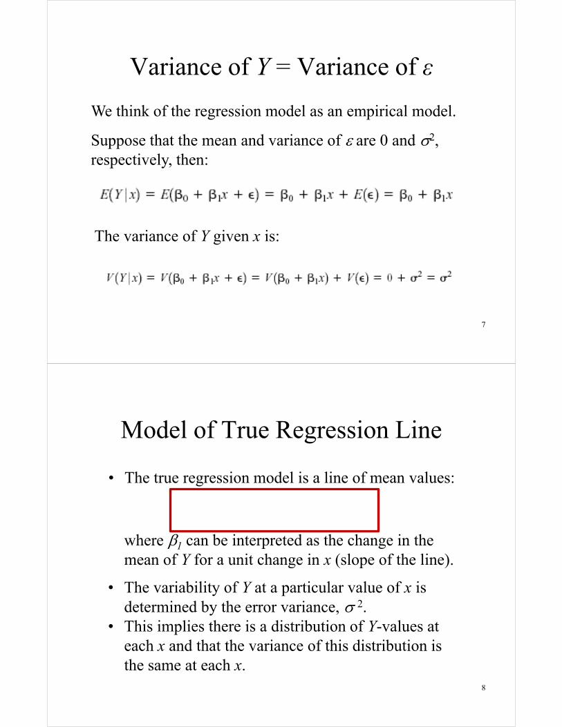
We think of the regression model as an empirical model.
Suppose that the mean and variance of � are 0 and �2, respectively, then:
The variance of Y given x is:
Variance of Y = Variance of ε
7
• The true regression model is a line of mean values:
where �1 can be interpreted as the change in the mean of Y for a unit change in x (slope of the line).
• The variability of Y at a particular value of x is determined by the error variance, � 2.
• This implies there is a distribution of Y-values at each x and that the variance of this distribution is the same at each x.
Model of True Regression Line
8
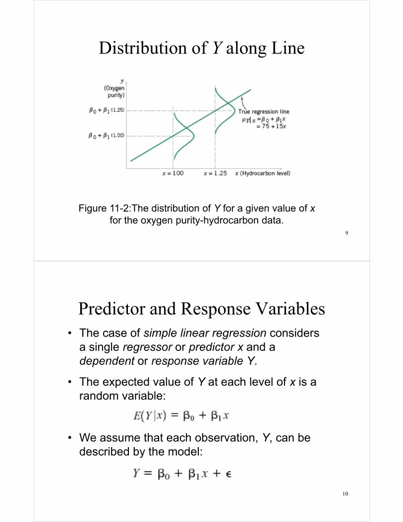
Figure 11-2:The distribution of Y for a given value of x for the oxygen purity-hydrocarbon data.
Distribution of Y along Line
9
• The case of simple linear regression considers a single regressor or predictor x and a dependent or response variable Y.
• The expected value of Y at each level of x is a random variable:
• We assume that each observation, Y, can be described by the model:
Predictor and Response Variables
10

• Suppose that we have n pairs of observations (x1, y1), (x2, y2), … (xn, yn). The method of least squares is used to estimate the parameters, �0 and �1, by minimizing the sum of the squares of the vertical deviations.
Figure 11-3: Deviations of the data from the estimated regression model.
Method of Least Squares
11
• Since the n observations in the sample can be expressed as:
• The sum of the squares of the deviations (errors) of the observations from the true regression line is:
Sum of Square Deviations
12

Least Squares Normal Equations
13
Simple Linear Regression Coefficients
14

Fitted Regression Line
15
16
� �n
xxxxS
n
iin
ii
n
iixx
2
1
1
2
1
2��
�
�
� ��
�� �
��
� �� �n
yxyxxxyyS
n
ii
n
ii
i
n
iii
n
iixy
��
�
���
�
�
� ���
�� ��
��
11
11
Sums of Squares The following notation may also be used:
Then,
xx
xy
SS
�1̂� xy 10ˆˆ �� �and
(11-10)
(11-11)
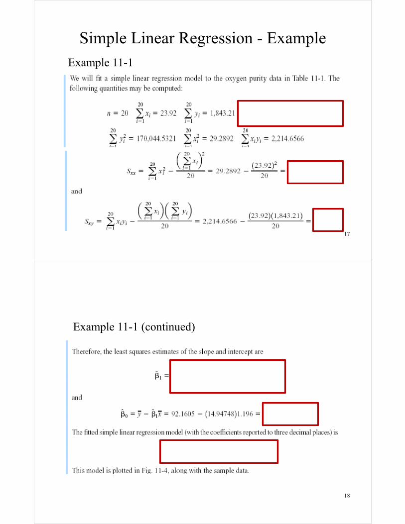
Example 11-1
Simple Linear Regression - Example
17
Example 11-1 (continued)
18
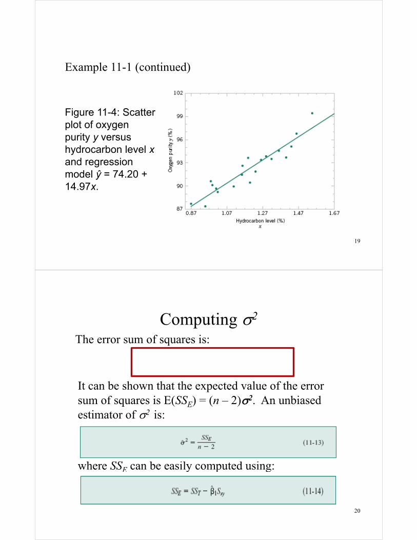
Figure 11-4: Scatter plot of oxygen purity y versus hydrocarbon level x and regression model ŷ = 74.20 + 14.97x.
Example 11-1 (continued)
19
where SSE can be easily computed using:
Computing �2
20
The error sum of squares is:
It can be shown that the expected value of the error sum of squares is E(SSE) = (n – 2)��2. An unbiased estimator of �2 is:
21
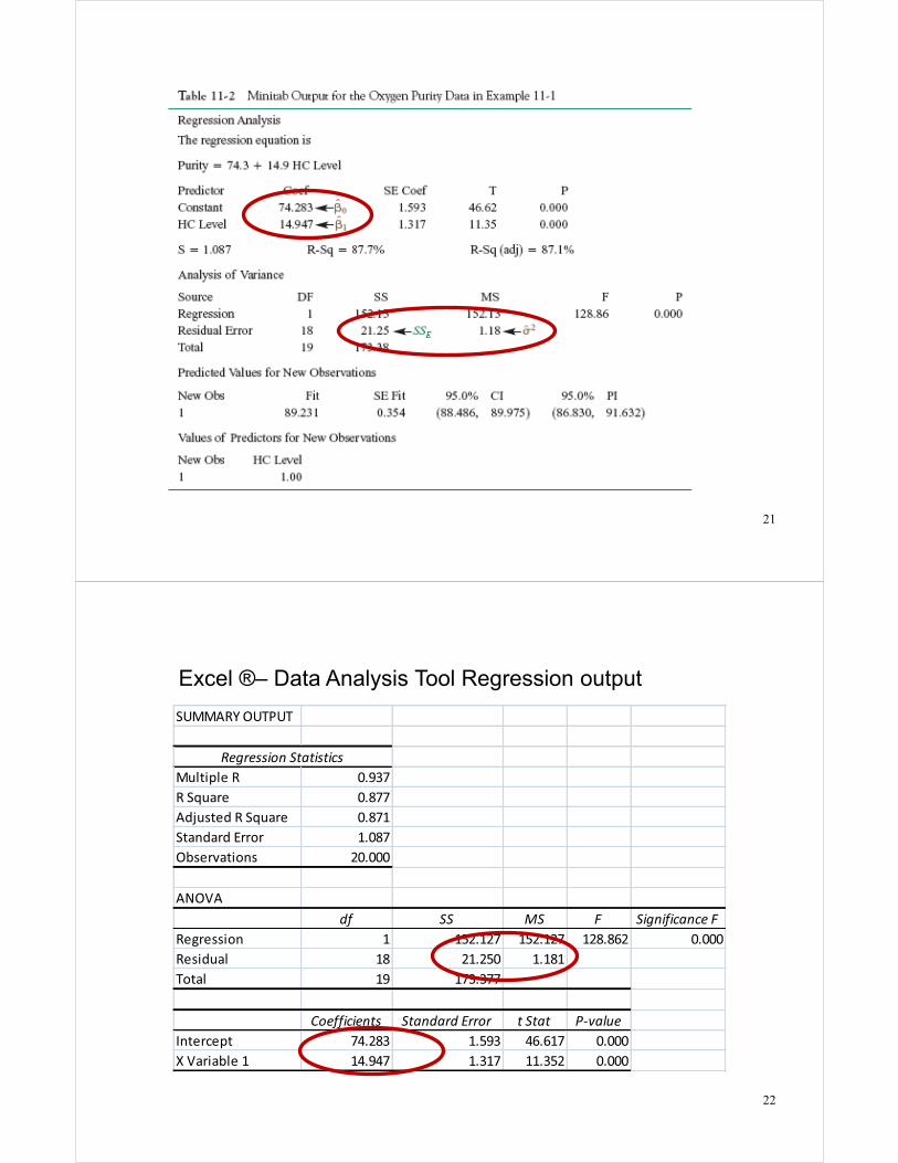
22
SUMMARY OUTPUT
Regression StatisticsMultiple R 0.937R Square 0.877Adjusted R Square 0.871Standard Error 1.087Observations 20.000
ANOVAdf SS MS F Significance F
Regression 1 152.127 152.127 128.862 0.000Residual 18 21.250 1.181Total 19 173.377
Coefficients Standard Error t Stat P-valueIntercept 74.283 1.593 46.617 0.000X Variable 1 14.947 1.317 11.352 0.000
Excel ®– Data Analysis Tool Regression output

• Slope properties for the mean and variance
• Intercept properties for the mean and variance
Properties of Least Squares Estimators
23
(11-15)
(11-16)
(11-17)
24
In simple linear regression the estimated standard error of the slope and the estimated standard error of the intercept are:
respectively, where the estimated variance is computed using Equation 11-13.
� �xxS
se2
1ˆˆ �� � � � �
�
���
���
xxSx
nse
22
01ˆˆ ��
• Estimated Standard Errors
If we wish to test the slope is some value β1,0:
An appropriate test statistic would be:
Hypothesis Test for the Slope
� �1
0,11
2
0,110 ˆ
ˆ
ˆ
ˆ
���
�
��seS
TXX
�
�
We would reject the null hypothesis if:
25
(11-18)
(11-19)
(11-20)
If we wish to test the intercept is some value β0,0:
An appropriate test statistic would be:
Hypothesis Test for the Intercept
We would reject the null hypothesis if:
26
(11-21)
(11-22)

Significance of Regression
An important special case of these hypotheses is:
Failure to reject H0 is equivalent to concluding that there is no linear relationship between x and Y.
In other words, if we conclude the slope could be 0 the information on x tells us nothing about the variation in the response, Y.
27
(11-23)
Figure 11-5: The hypothesis H0: �1 = 0 is not rejected.
Figure 11-6: The hypothesis H0: �1 = 0 is rejected. 28
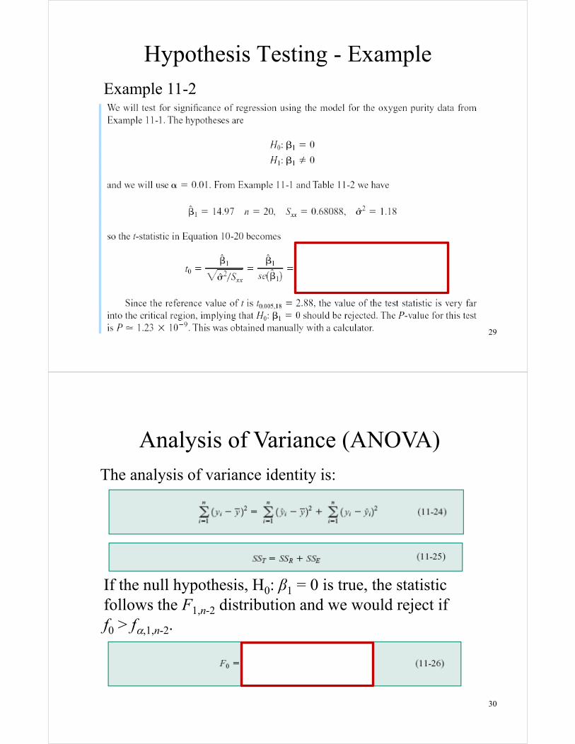
Hypothesis Testing - Example Example 11-2
29
The analysis of variance identity is:
30
Analysis of Variance (ANOVA)
If the null hypothesis, H0: β1 = 0 is true, the statistic follows the F1,n-2 distribution and we would reject if f0 > f�,1,n-2.

The quantities MSR and MSE are called mean squares of the regression and the errors, respectively.
Analysis of variance (ANOVA) table:
31
The ANOVA Table
32
Example 11-3 Analysis of Variance - Example
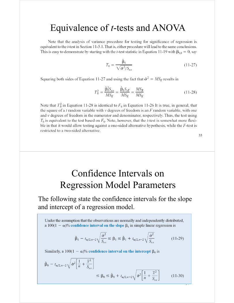
Equivalence of t-tests and ANOVA
33
34
Confidence Intervals on Regression Model Parameters
The following state the confidence intervals for the slope and intercept of a regression model.
35
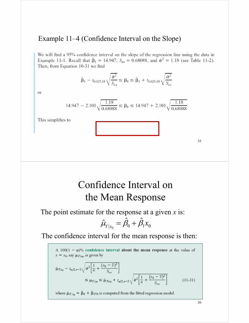
12.181 ≤ β1 ≤ 17.713
Example 11–4 (Confidence Interval on the Slope)
36
010ˆˆˆ
0xxY ��� ��
Confidence Interval on the Mean Response
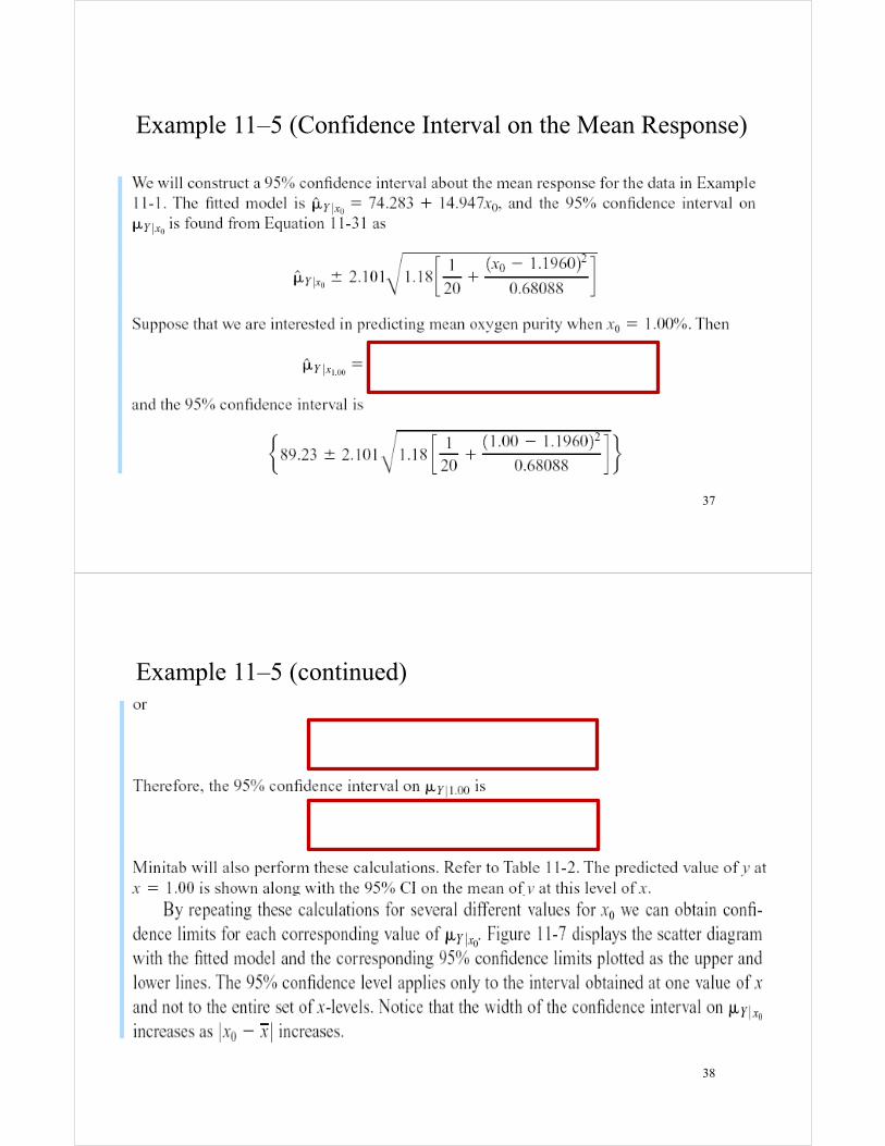
The point estimate for the response at a given x is:
The confidence interval for the mean response is then:
37
Example 11–5 (Confidence Interval on the Mean Response)
38
Example 11–5 (continued)
39
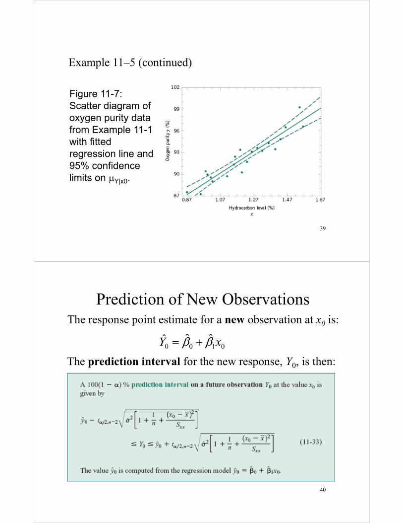
Figure 11-7: Scatter diagram of oxygen purity data from Example 11-1 with fitted regression line and 95% confidence limits on �Y|x0.
Example 11–5 (continued)
40
0100ˆˆˆ xY �� ��
Prediction of New Observations The response point estimate for a new observation at x0 is:
The prediction interval for the new response, Y0, is then:

41
Example 11–6 (Prediction Interval)
42
Example 11–6 (continued)

43
Figure 11-8: Scatter diagram of oxygen purity data from Example 11-1 with fitted regression line, 95% prediction limits (outer lines) , and 95% confidence limits on �Y|x0.
Example 11–6 (continued)
• Fitting a regression model requires several assumptions.
1. Errors are uncorrelated random variables with mean zero;
2. Errors have constant variance; and,
3. Errors be normally distributed.
• The analyst should always consider the validity of these assumptions to be doubtful and conduct analyses to examine the adequacy of the model
Adequacy of Regression Models
44

• The residuals from a regression model are ei = yi - ŷi , where yi is an actual observation and ŷi is the corresponding fitted value from the regression model.
• Analysis of the residuals is frequently helpful in checking the assumption that the errors are approximately normally distributed with constant variance, and in determining whether additional terms in the model would be useful.
Residual (Error) Analysis
45
Figure 11-9: Patterns for residual plots. (a) satisfactory, (b) funnel, (c) double bow, (d) nonlinear.
Residual Plots
46
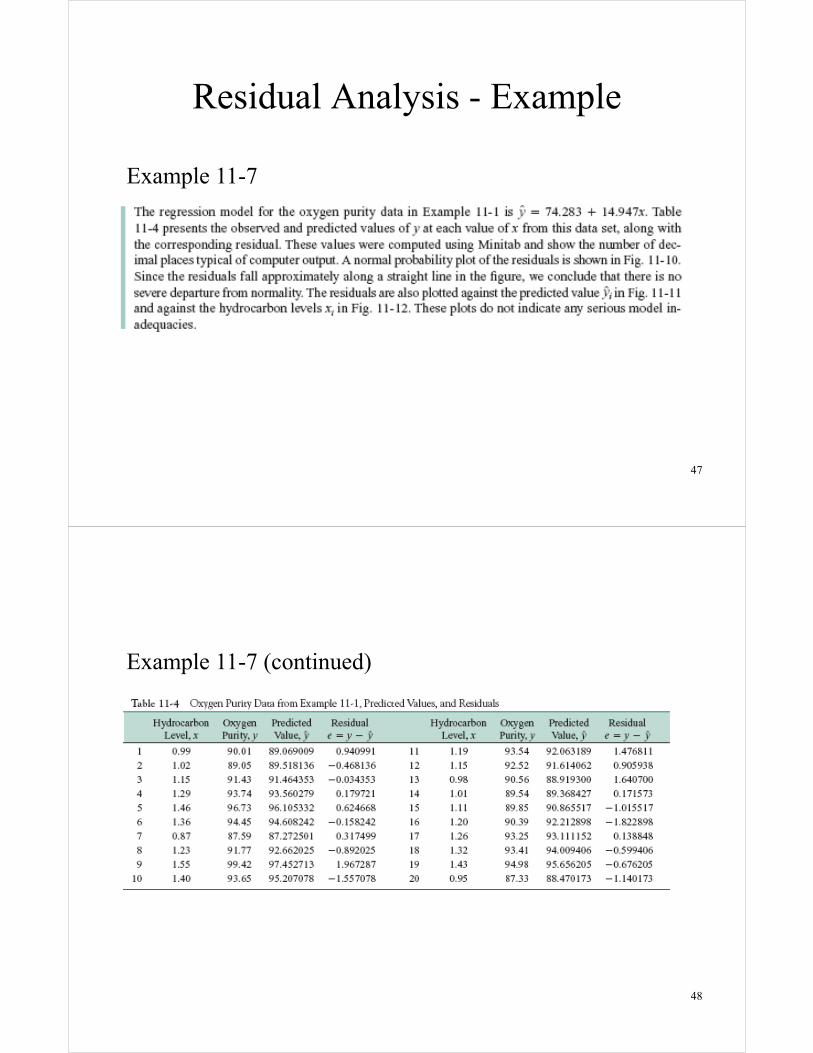
Example 11-7
Residual Analysis - Example
47
Example 11-7 (continued)
48

Figure 11-10: Normal probability plot of residuals, Example 11-7.
Example 11-7 (continued)
49
Figure 11-11: Plot of residuals versus predicted oxygen purity, ŷ, Example 11-7.
Example 11-7 (continued)
50

• The quantity
is called the coefficient of determination and is often used to judge the adequacy of a regression model.
• 0 � R2 � 1;
• We often refer (loosely) to R2 as the amount of variability in the data explained or accounted for by the regression model.
Coefficient of Determination (R2)
51
(11-34)
• For the oxygen purity regression model,
R2 = SSR/SST
= 152.13/173.38
= 0.877
• Thus, the model accounts for 87.7% of the variability in the data.
R2 Computations - Example
52

53
Regression on Transformed Variables
In many cases a plot of the independent variable, y, against the dependent variable, x, may show the relationship is not linear.
Performing a linear regression would lead to a poor fit and residual analysis would show the model is inadequate.
However, we can often transform the dependent variable first. This transformed variable, x’, may have a linear relationship with y.
54
Therefore, we can perform a linear regression between the x’ and y.
However, note that any use of the new equation for prediction would require a reverse transformation to indicate the desired value of x. Transformation can take on many forms. Typical ones include: x’ = logarithm (x) x’ = square root (x) x’ = inverse (x).

55
Obs. Output (y) Velocity (x) x'=1/x
1 1.582 5.00 0.2002 1.822 6.00 0.1673 1.057 3.40 0.2944 0.5 2.70 0.3705 2.236 10.00 0.1006 2.386 9.70 0.1037 2.294 9.55 0.1058 0.558 3.05 0.3289 2.166 8.15 0.123
10 1.866 6.20 0.16111 0.653 2.90 0.34512 1.93 6.35 0.15713 1.562 4.60 0.21714 1.737 5.80 0.17215 2.088 7.40 0.13516 1.137 3.60 0.27817 2.179 7.85 0.12718 2.112 8.80 0.11419 1.8 7.00 0.14320 1.501 5.45 0.18321 2.303 9.10 0.11022 2.31 10.20 0.09823 1.194 4.10 0.24424 1.144 3.95 0.25325 0.123 2.45 0.408
Example 11-9
An engineer has collected data on the DC output from a windmill under different wind speed conditions. He wishes to develop a model describing output in terms of wind speed.
The table on the right shows the data collected for output, y, as a response and wind speed, x, as the dependent variable.
The final column shows the transformed value, x’=1/x.
56
Example 11-9 (continued)
Regression Equation (Original Data): y = 0.1309 + 0.2411 x
R2 = 0.875
0.0
0.5
1.0
1.5
2.0
2.5
3.0
0 2 4 6 8 10 12
DC
Out
put
Wind Velocity, x
Original

57
Example 11-9 (continued)
Regression Equation (Transformed Data): y = 2.9789 – 6.9345 x’
R2 = 0.980
0.0
0.5
1.0
1.5
2.0
2.5
3.0
0.0 0.1 0.2 0.3 0.4 0.5
DC
Out
put
Transformed Wind Velocity, 1/x
Transformed
58
THE END OF ENGG 319 CLASS NOTES


