Embed Size (px)
Citation preview

2 3 4 5
3
4
5
6
7
8
9
10
x
y
Chapter 11 Handout
Scatter Plots and Correlation
Bivariate Data x1 , y1 , x2 , y2 , …, xn , yn
Scatter plot A picture of bivariate numerical data in which each observation x i , yi is represented as a point locatedwith respect to a horizontal x axis and a vertical y axis
Example
x y2 33 64 75 10
Things to Notice About Bivariate Data and Scatter Plots:1. The relationship between y and x.
• Positive Relationship: y increases as x increases • Negative Relationship: y decreases as x increases• No Relationship
2. Does it appear that the value of y can be predicted from knowing x by finding a line that is reasonably closeto the points in the plot?
Correlation Coefficient a quantitative assessment of the strength of the relationship between the x's and y's
Pearson's Sample Correlation Coefficient r=∑ xi−x yi−y
∑ xi−x 2∑ yi−y 2=
S xy
S xx S yy
The following are an alternative way to compute the above quantities.
S xx=∑ x i2−
∑ x i 2
nS yy=∑ yi
2−∑ yi
2
nS xy=∑ x i yi−
∑ x i ∑ yi n
Properties of r
• The value of r does not depend on the unit of measurement for either variable. It is unitless. For example, if x isdistance, r will not change regardless of whether x is measured in feet, yards, miles, or any other unit.
• The value of r does not depend on which of the two variables is labeled x.• The value of r is between 1 and +1.
• r close to +1 indicates a strong positive linear relationship• r close to 1 indicates a strong negative linear relationship• r close to 0 indicates a very weak linear relationship or no linear relationship at all• r = +1 only when all the points in the scatter plot lie exactly on a straight line that slopes upward• r = 1 only when all the points in the scatter plot lie exactly on a straight line that slopes downward
• The value of r is a measure of the extent to which x and y are linearly related (straight line) only. A value of rclose to zero means x and y are not linearly related. It doesn’t mean that x and y are unrelated.
ST361 1 Chp 11 Handout

3 4 5 6 7
5
6
7
8
9
10
11
12
13
14
x
y2
3 4 5 6 7
6
78
910
111213
1415
16
x
y3
3 4 5 6 7
5
6
7
8
9
10
11
12
13
14
x
y1
3 4 5 6 7
14
13
12
11
10
9
8
7
6
5
x
y5
3 4 5 6 7
16
1514
1312
1110
9
87
6
x
y4
76543
5
4
3
2
1
0
x
y6
Chapter 11 Handout
• r is the square root of the quantity R2 (or Rsquared) in computer output• Strength of r :
strong moderate weak moderate strong
1.0 0.8 0.5 0.0 0.5 0.8 1.0
Examples
Exact line (r = 1) Positive correlation (r = .8) No relationship (r = .003)
Exact line (r = 1) Negative correlation (r = .8) No correlation (r = .003)
Note: When examining a scatter plot you should be able to do the following:• Determine if there is a relationship between the two variables, x and y• If there is a relationship, be able to describe it’s shape, direction, and strength of r
Population Correlation Coefficient ( ρ) :
• The Pearson's sample correlation coefficient (r) is an estimate of the population correlation coefficient (ρ)• ρ is a number between 1 and +1• ρ is unitless (the value of ρ does not depend on the unit of measurement for either variable) • ρ = +1 or 1 only if all (x, y) pairs in the population lie exactly on a straight line• ρ measures the extent to which there is a linear relationship in the population
• = xy
x y
, where xy2 =∫ xy−xy f x , ydx dy is the Covariance between x and y.
f (x , y) is a bivariate or joint density for the variables x and y.
ST361 2 Chp 11 Handout
Chapter 11 Handout
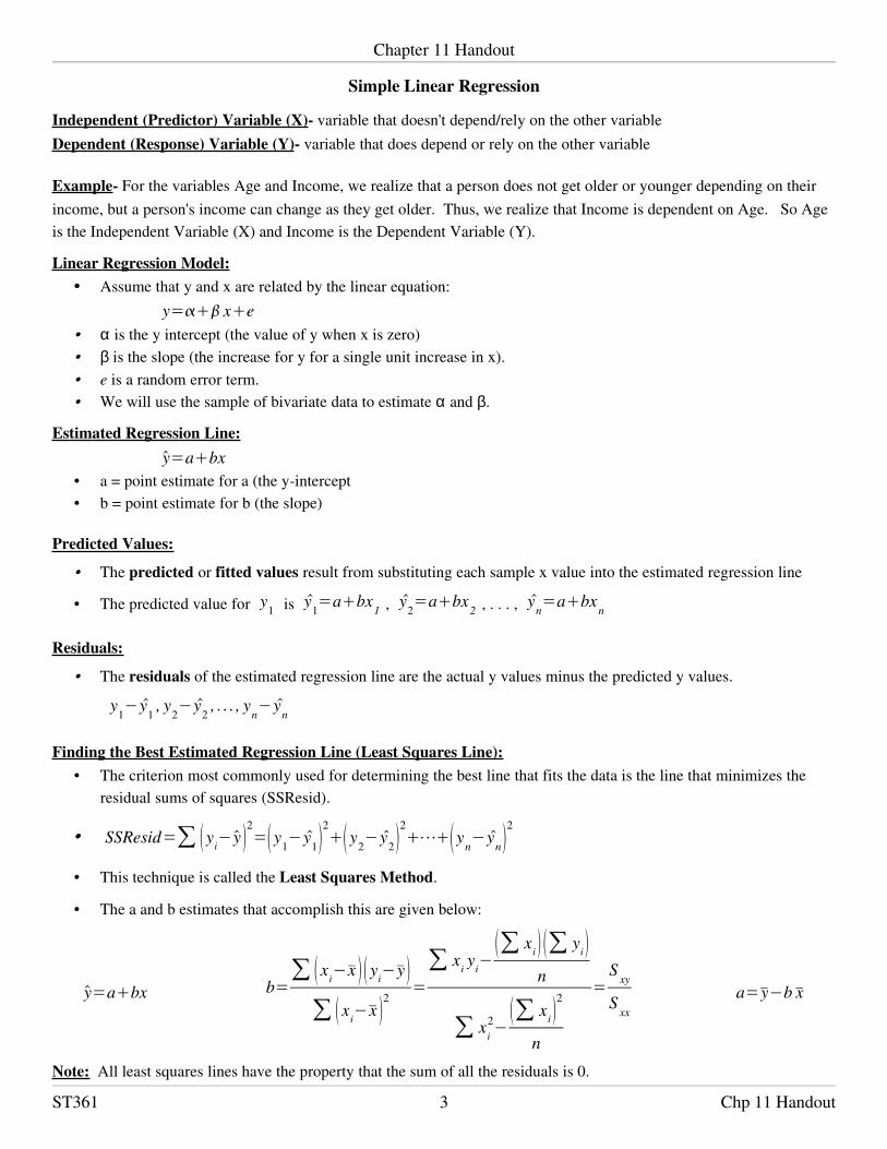
Simple Linear Regression
Independent (Predictor) Variable (X) variable that doesn't depend/rely on the other variableDependent (Response) Variable (Y) variable that does depend or rely on the other variable
Example For the variables Age and Income, we realize that a person does not get older or younger depending on theirincome, but a person's income can change as they get older. Thus, we realize that Income is dependent on Age. So Ageis the Independent Variable (X) and Income is the Dependent Variable (Y).
Linear Regression Model:• Assume that y and x are related by the linear equation:
y= xe• α is the y intercept (the value of y when x is zero)• β is the slope (the increase for y for a single unit increase in x).• e is a random error term.• We will use the sample of bivariate data to estimate α and β.
Estimated Regression Line:y=abx
• a = point estimate for a (the yintercept• b = point estimate for b (the slope)
Predicted Values:• The predicted or fitted values result from substituting each sample x value into the estimated regression line
• The predicted value for y1 is y1=abx1 , y2=abx2 , . . . , yn=abxn
Residuals:• The residuals of the estimated regression line are the actual y values minus the predicted y values.
y1− y1 , y2− y2 , . . . , yn− yn
Finding the Best Estimated Regression Line (Least Squares Line):• The criterion most commonly used for determining the best line that fits the data is the line that minimizes the
residual sums of squares (SSResid).
• SSResid=∑ yi−y 2=y1− y12 y2− y2
2⋯yn− yn
2
• This technique is called the Least Squares Method.
• The a and b estimates that accomplish this are given below:
y=abx b=∑ xi−x yi−y ∑ xi−x 2
=∑ xi yi−
∑ xi ∑ yi n
∑ xi2−
∑ xi 2
n
=S xy
S xx a=y−b x
Note: All least squares lines have the property that the sum of all the residuals is 0.
ST361 3 Chp 11 Handout

Chapter 11 Handout
Prediction: • A predicted y value for any x value can be obtained by plugging x value into the least squares line equation
Ex the least squares line for a sample is y=1225 x . What is the predicted value for x = 4?
y=1225 x =1225 4 =12100=112• Don’t ever make a prediction for an x value outside the range of the x’s. This is called Extrapolation.
Ex If I had only collected data for the example above for x’s between 0 and 20, I cannot make a predictionfor x = 30 which is outside the range of my x’s.
Coefficient of Determination the proportion of variation in y that can be explained by a linear relationship between xand y.
• Residual Sum of Squares (measure of unexplained variation) denoted SSResid is given by:
SSResid=∑ y−y 2=y1− y12 y2− y2
2⋯yn− yn
2=S yy−b S xy
• Total Sum of Squares (measure of total variation) denoted SSTo is given by:
SSTo=∑ y−y 2= y1− y12 y2− y2
2⋯ yn− yn
2=∑ yi
2−∑ yi
2
n=S yy
• Coefficient of Determination denoted r2 is given by: r2=SSTo−SS Re sid
SSTo• r2=correlation 2 . This is why we call the coefficient of determination r2
• High values of r2 (like 0.9 or higher) indicate that a line is a pretty good model for the relationship between xand y.
Standard Deviation About the Least Squares Line: se= SSResidn−2
Hypothesis testing in Regression:• Recall that we are assuming that the relationship between x and y is defined by the equation
y= xe• We can test whether or not there is a linear relationship by testing whether or not the slope equals 0.
Ho: β = 0 vs. Ha: β ≠ 0
• In order to perform this test we need to make the assumption that e~N 0, at every x value.• Then if Ho is true (β= 0),
t= bsb
has a t distribution with n2 d.f.
Where sb=se
S xx
( sb is given in the computer printout along with t and the pvalue for the test)
Confidence Interval for β : • When the normality and equal variance assumptions made above hold, then a (1α)100% CI for β is:
b±t n−2* sb
ST361 4 Chp 11 Handout
Chapter 11 Handout
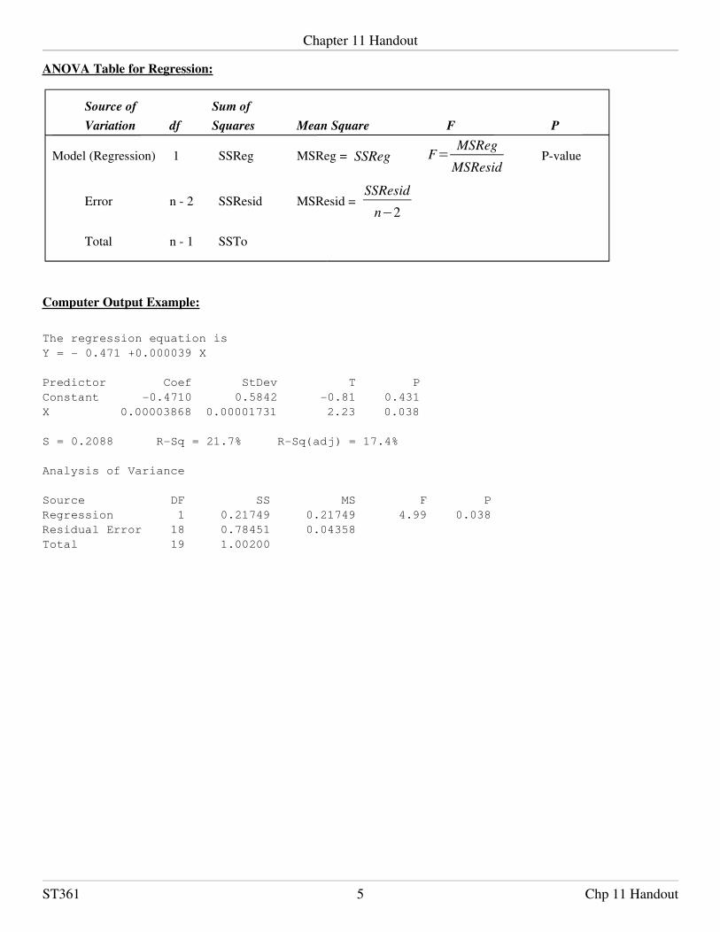
ANOVA Table for Regression:
Source of Sum ofVariation df Squares Mean Square F P
Model (Regression) 1 SSReg MSReg = SSReg F=MSReg
MSResid Pvalue
Error n 2 SSResid MSResid = SSResid
n−2
Total n 1 SSTo
Computer Output Example:
The regression equation isY = 0.471 +0.000039 X
Predictor Coef StDev T PConstant 0.4710 0.5842 0.81 0.431X 0.00003868 0.00001731 2.23 0.038
S = 0.2088 RSq = 21.7% RSq(adj) = 17.4%
Analysis of Variance
Source DF SS MS F PRegression 1 0.21749 0.21749 4.99 0.038Residual Error 18 0.78451 0.04358Total 19 1.00200
ST361 5 Chp 11 Handout