Embed Size (px)
Citation preview

Chapter 10: Emissions from Livestoch and Manure Management
2019 Refinement to the 2006 IPCC Guidelines for National Greenhouse Gas Inventories 10.1
CH APTE R 10
EMISSIONS FROM LIVESTOCK AND
MANURE MANAGEMENT

Volume 4: Agriculture, Forestry and Other Land Use
10.2 2019 Refinement to the 2006 IPCC Guidelines for National Greenhouse Gas Inventories
Authors:
Olga Gavrilova (Estonia), Adrian Leip (EU), Hongmin Dong (China), James Douglas MacDonald (Canada),
Carlos Alfredo Gomez Bravo (Peru), Barbara Amon (Germany), Rolando Barahona Rosales (Honduras), Agustin
del Prado (Spain), Magda Aparecida de Lima (Brazil), Walter Oyhantçabal (Uruguay), Tony John van der
Weerden (New Zealand), Yeni Widiawati (Indonesia)
Contributing Authors:
Andre Bannink (Netherlands), Karen Beauchemin (Canada), Harry Clark (New Zealand), April Leytem (USA),
Ermias Kebreab (USA), Ngwa Martin Ngwabie (Cameroon), Carolyn Imede Opio (Uganda), Andrew VanderZaag
(Canada), Theunis Valentijn Vellinga (Netherlands)

Chapter 10: Emissions from Livestoch and Manure Management
2019 Refinement to the 2006 IPCC Guidelines for National Greenhouse Gas Inventories 10.3
Contents
10. Emissions from livestock and manure management ................................................................................ 10.9
10.1 Introdouction ...................................................................................................................................... 10.9
10.2 Livestock population and feed characterisation ............................................................................... 10.10
10.2.1 Steps to define categories and subcategories of livestock ..................................................... 10.10
10.2.2 Choice of method .................................................................................................................. 10.10
10.2.3 Uncertainty assessment ......................................................................................................... 10.31
10.2.4 Characterisation for livestock without species: Specific emission estimation methods ........ 10.32
10.3 Methane emissions from enteric fermentation ................................................................................. 10.33
10.3.1 Choice of method .................................................................................................................. 10.33
10.3.2 Choice of emission factors .................................................................................................... 10.35
10.3.3 Choice of activity data .......................................................................................................... 10.48
10.3.4 Uncertainty assessment ......................................................................................................... 10.48
10.3.5 Completeness, Time series, Quality Assurance/Quality Control and Reporting .................. 10.48
10.4 Methane Emissions from Manure Management............................................................................... 10.49
10.4.1 Choice of method .................................................................................................................. 10.49
10.4.2 Choice of emission factors .................................................................................................... 10.53
10.4.3 Choice of activity data .......................................................................................................... 10.71
10.4.4 Uncertainty assessment ......................................................................................................... 10.73
10.4.5 Completeness, Time series, Quality assurance / Quality control and Reporting .................. 10.73
10.5 N2O Emissions from Manure Management ..................................................................................... 10.74
10.5.1 Choice of method .................................................................................................................. 10.74
10.5.2 Choice of emission factors .................................................................................................... 10.80
10.5.3 Choice of activity data .......................................................................................................... 10.93
10.5.4 Coordination with reporting for N2O emissions from managed soils ................................... 10.93
10.5.5 Uncertainty assessment ......................................................................................................... 10.99
10.5.6 Completeness, Time series, Quality assurance/Quality control and Reporting .................... 10.99
10.5.7 Use of worksheets ............................................................................................................... 10.102
Annex 10A.1 Data underlying methane default emission factors for enteric fermentation, volatile
solids and nitrogen excretion and retention fractions for Cattle and Buffalo ..... 10.103
Annex 10A.2 Additional data and information for the calculation of methane and nitrous oxide from
Manure Management ......................................................................................... 10.117
Annex 10A.3 Spreadsheet example for the calculation of a country or regions specific MCF 10.133
Annex 10A.4 Calculations of Methane Conversion Factors (MCFs) factors for biogas
systems ............................................................................................................... 10.141
Annex 10A.5 Equations relating all direct and indirect N2O emissions from manure along all stages
in agricultural production for livestock .............................................................. 10.146
Annex 10B Data and Explanatory Text for Development of New Parameters in the 2019
Refinement.......................................................................................................... 10.152

Volume 4: Agriculture, Forestry and Other Land Use
10.4 2019 Refinement to the 2006 IPCC Guidelines for National Greenhouse Gas Inventories
10B.1 Raw data used to compile Annex A.1 enteric fermentation Tier 1 emission factors,
volatile solids and nitrogen excretion for cattle and buffalo .............................. 10.152
10B.2 Estimation Cattle/Buffalo CH4 conversion factors (Ym) .................................... 10.156
10B.3 Estimation of Default Emission Factor(s) for Goat Tier 2 parameters ............... 10.159
10B.4 Feed intake estimates using a simplified Tier 2 method .................................... 10.163
10B.5 Basis for Changes to MCF Calculations for Liquid/Slurry ................................ 10.164
10B.6 Revision of methane from dung deposited onto pasture range and paddocks .... 10.167
10B.7 Estimation of default emission factors for MCF CH4 values, EF for direct N2O
emissions, NH3, NO3 leaching and N2 emissions from solid storage and composting
systems ............................................................................................................... 10.168
References ........................................................................................................................... 10.172
References Annexes ........................................................................................................................... 10.180
Equations
Equation 10.1 (Updated) Annual average population .................................................................................. 10.11
Equation 10.2 Coefficient for calculating net energy for maintenance ....................................... 10.19
Equation 10.3 Net energy for maintenance ................................................................................. 10.22
Equation 10.4 Net energy for activity (for cattle and buffalo) .................................................... 10.23
Equation 10.5 Net energy for activity (for sheep and goats) ....................................................... 10.23
Equation 10.6 Net energy for growth (for cattle and buffalo) ..................................................... 10.24
Equation 10.7 Net energy for growth (for sheep and goats) (updated) ....................................... 10.25
Equation 10.8 Net energy for lactation (for beef cattle, dairy cattle and buffalo) ....................... 10.25
Equation 10.9 (Updated) Net energy for lactation for sheep and goats (milk production known) .............. 10.26
Equation 10.10 Net energy for lactation for sheep and goats (milk production unknown) ........... 10.26
Equation 10.11 Net energy for work (for cattle and buffalo) ........................................................ 10.26
Equation 10.12 (Updated) Net energy to produce wool (for sheep and goats) ............................................... 10.27
Equation 10.13 (Updated) Net energy for pregnancy (for cattle/buffalo and sheep and goats) .................... 10.27
Equation 10.14 Ratio of net energy available in a diet for maintenance to digestible energy ....... 10.28
Equation 10.15 Ratio of net energy available for growth in a diet to digestible energy
consumed ............................................................................................................. 10.29
Equation 10.16 Gross energy for cattle/buffalo, sheep and goats ................................................. 10.29
Equation 10.17 (Updated) Estimation of dry matter intake for calves .......................................................... 10.30
Equation 10.18 (Updated) Estimation of dry matter intake for growing cattle ............................................. 10.30
Equation 10.18a (Updated) Estimation of dry matter intake for steers and bulls ............................................ 10.30
Equation 10.18b (Updated) Estimation of dry matter intake for lactating dairy cows .................................... 10.31
Equation 10.19 (Updated) Enteric fermentation emissions from a livestock category (Tier 1) .................... 10.38
Equation 10.20 (Updated) Total emissions from livestock enteric fermentation (Tier 1) .............................. 10.38
Equation 10.21 Methane emission factors for enteric fermentation from a livestock category .... 10.46
Equation 10.21a (New) Methane emission factors for enteric fermentation from a livestock category .... 10.46

Chapter 10: Emissions from Livestoch and Manure Management
2019 Refinement to the 2006 IPCC Guidelines for National Greenhouse Gas Inventories 10.5
Equation 10.22 (Updated) CH4 emissions from manure management (Tier 1) .............................................. 10.53
Equation 10. 22a (Updated) Annual VS excretion rates (Tier 1) ...................................................................... 10.54
Equation 10.23 CH4 emission factor from manure management .................................................. 10.63
Equation 10.24 (Updated) Volatile solid excretion rates ............................................................................... 10.64
Equation 10.25 (Updated) Direct N2O emissions from manure management ............................................... 10.75
Equation 10.26 (Updated) N losses due to volatilisation from manure management ..................................... 10.76
Equation 10.27 (Updated) N losses due to leaching from manure management ........................................... 10.77
Equation 10.28 Indirect N2O emissions due to volatilisation of N from manure management ..... 10.78
Equation 10.29 Indirect N2O emissions due to leaching from manure management .................... 10.78
Equation 10.30 (Updated) Annual N excretion rates ..................................................................................... 10.80
Equation 10.31 Annual N excretion rates, Option 1 (Tier 2) ........................................................ 10.81
Equation 10.31a (New) Annual N excretion rates, Option 2 (Tier 2) ........................................................ 10.81
Equation 10.32 N intake rates for cattle, Sheep and Goats ........................................................... 10.82
Equation 10. 32a (New) N intake rates for swine and poultry .................................................................... 10.82
Equation 10.33 N retention rates for cattle .................................................................................... 10.85
Equation 10.33a (New) N retention rates for breeding sows ..................................................................... 10.86
Equation 10.33b (New) N retention rates for piglets .................................................................................. 10.86
Equation 10.33c (New) N retention rates for growing pigs ....................................................................... 10.87
Equation 10.33d (New) N excretion rates for layer type hens .................................................................... 10.88
Equation 10.33e (New) Annual N retention rates for pullets or broilers ................................................... 10.88
Equation 10.34 (Updated) Managed manure N available for application to managed soils, feed, fuel or
construction uses ................................................................................................. 10.94
Equation 10.34a (New) Managed manure N available for application to managed soils or for the production
of feed, fuel or for construction uses ................................................................... 10.94
Equation 10.34b (New) Estimation of fracN2ms ......................................................................................... 10.95
Equation 10A.1 (New) Calculation of MCF for the combination “digester + digestate storage” ........... 10.141
Equation 10A.2 (New) Calculation of relative amount of potential off gas related to B0 ....................... 10.142
Equation 10A.3 (New) Calculation of relative amount of residual gas related to B0 ............................. 10.142
Equation 10A.4 (New) Calculation of relative amount of residual gas related to CH4 production ........ 10.142
Equation 10A.5 (New) Digester’s methane balance ............................................................................... 10.143
Equation 10A.6 (New) Calculation of methane leakage rate of digester ............................................... 10.143
Equation 10A.7 (New) Calculation of methane conversion factor ......................................................... 10.143
Equation 10A.8 (New) Calculation of methane conversion factor of residues ...................................... 10.144
Equation 10A.9 (New) Calculation of methane conversion factor for the combination “prestorage + digester
+ digestate storage” ........................................................................................... 10.144
Equation 10A.10 (New) Total N2O emissions for animal type t .............................................................. 10.146
Equations 10A.11 and 10A.12 (New) Total N2O emissions from manure management for animal type
t .................................................................................................... 10.146
Equations 10A.13 through 10A.14 (New) Total, direct and indirect N2O emissions from the application of manure
to managed soils for animal type t .............................................. 10.146
Equation 10A.15 (New) Total amount of animal manure N applied to soils other than by grazing animals for
animal type t ...................................................................................................... 10.147

Volume 4: Agriculture, Forestry and Other Land Use
10.6 2019 Refinement to the 2006 IPCC Guidelines for National Greenhouse Gas Inventories
Equation 10A.16 (New) Fraction of total animal manure N lost in manure management systems for animal
type t ................................................................................................................. 10.147
Equation 10A.17 (New) Fraction of animal manure N available for application to managed soils, applied to
managed soils for animal type t ......................................................................... 10.147
Equation 10A.18 through 10A.19 (New) Total, direct and indirect N2O emissions from n in urine and dung
deposited by grazing animals on pasture, range and paddock (Tier 1)
for animal type t ........................................................................... 10.147
Equation 10A.20 (New) Relationship between average annual nitrogen flows associated with an individual
animal [kg N animal-1 yr-1] and the annual nitrogen flow for the animal population of
livestock category/species t in a country [kg N yr-1] ......................................... 10.147
Equation 10A.21 (New) Total manure-N excreted ................................................................................... 10.148
Equation 10A.22 and 10A.23 (New) Nitrogen excretion calculated either using a default fraction of retention
(Tier 1) or directly from retention data ....................................... 10.148
Equation 10A.24 (New) Total manure-N in manure management and storage systems .......................... 10.148
Equation 10A.25 (New) Manure-N managed in system S ........................................................................ 10.148
Equation 10A.26 (New) Manure-N deposited by grazing animals, with X=CPP,SO ............................... 10.148
Equation 10A.27 (New) N in bedding material added to managed manure .............................................. 10.148
Figures
Figure 10.1 Decision tree for livestock population characterisation ....................................... 10.12
Figure 10.2 (Updated) Decision Tree for CH4 Emissions from Enteric Fermentation ............................. 10.34
Figure 10.3 (Updated) Decision tree for CH4 emissions from Manure Management............................... 10.52
Figure 10.4 (Updated) Decision tree for N2O emissions from Manure Management .............................. 10.79
Figure 10.5 (New) Processes leading to the emission of gaseous N species from manure .............. 10.102
Figure 10A.1 (New) Mapping of IPCC climate zones ........................................................................ 10.130
Figure 10A.2 (New) Colour code for cells in the example spreadsheet. ............................................. 10.133
Figure 10A.3 (New) Temperature and manure removal inputs to the model. ..................................... 10.135
Figure 10A.4 (New) Constants and other input parameters for the model .......................................... 10.136
Figure 10A.5 (New) Monthly model inputs and outputs over a three year period. ............................. 10.137
Figure 10A.6 (New) Formulae used in the model. ..................................... Error! Bookmark not defined.
Figure 10A.7 (New) Example of monthly patterns in Year 3: manure temperature, VS available (kg), VS
emptied (kg), and methane production. .............................................................. 10.139
Figure 10A.8 (New) Summary of Year 3 VS and methane production, and calculation of MCF. Top panel
shows results, bottom panel shows equations. ................................................... 10.139
Figure 10B.1 (New) Relationships between mean and median neutral detergent fibre (NDF) and methane
conversion rate (Ym) from summary statistics of Niu et al. (2018). ................... 10.157
Figure 10B.2 (New) Annual enteric methane output per animal expressed in mass in relation to daily dry
matter (DM) intake............................................................................................. 10.161
Figure 10B.3 (New) Daily enteric methane output per animal expressed in energy in relation to daily gross
energy (GE) intake. ............................................................................................ 10.161
Figure 10B.4 (New) Daily N excretion output per animal expressed in relation to animal weight. ... 10.161

Chapter 10: Emissions from Livestoch and Manure Management
2019 Refinement to the 2006 IPCC Guidelines for National Greenhouse Gas Inventories 10.7
Figure 10B.5 (New) Daily N excretion output per animal expressed in relation to daily N intake. .... 10.162
Figure 10B.6 (New) Comparison between ranges of CH4-C emissions observed in collected studies in
Pardo et al. (2015) (new) with estimations for the same studies according to IPCC
(2006) methodology. ..................................................................................... 10.10.169
Figure 10B.7 (New) Effect on cumulative NH3-N emissions of different solid storage and composting
methods compared with conventional solid storage. ..................................... 10.10.170
Tables
Table 10.1 (Updated) Representative livestock categories .................................................................... 10.15
Table 10.2 (Updated) Representative feed digestibility for various livestock categories ......................... 10.21
Table 10.3 (Updated) Summary of the equations used to estimate daily gross energy intake for cattle,
buffalo and sheep and goats ................................................................................... 10.22
Table 10.4 (Updated) Coefficients for calculating net energy for maintenance ( NEm ) .......................... 10.23
Table 10.5 (Updated) Activity coefficients corresponding to animal’s feeding situation ......................... 10.24
Table 10.6 (Updated) Constants for use in calculating neg for sheep and goats ........................................ 10.25
Table 10.7 (Updated) Constants for use in calculating NEp in Equation 10.13 ........................................ 10.28
Table 10.8 (New) DMI Required By Mature Non Dairy Cows Based On Forage Quality ................. 10.31
Table 10.8a (Updated) Examples of NEmf content of typical diets fed to cattle for estimation of dry matter
intake in equations 10.17 and 10.18 ...................................................................... 10.31
Table 10.9 (Updated) Suggested emissions inventory methods for enteric fermentation ......................... 10.36
Table 10.10 (Updated) Enteric fermentation emission factors for Tier 1 method (kg CH4 head-1 yr-1) ...... 10.37
Table 10.11 (Updated) Tier 1 and Tier 1a Enteric fermentation emission factors for Cattle and Buffalo ... 10.39
Table 10.12 (Updated) Cattle/buffalo methane conversion factors (Ym ) .................................................... 10.45
Table 10.13 (Updated) Sheep and goats ch4 conversion factors (Ym) ......................................................... 10.46
Table 10.13a (New) Default values for volatile solid excretion rate (kg VS (1,000 kg animal mass)-1 day-
1) ............................................................................................................................. 10.55
Table 10.14 (Updated) Methane Emission Factors by animal category, manure management system and
climate zone (g CH4 kg VS-1) ................................................................................ 10.57
Table 10.15 (Updated) Manure management methane emission factors for deer, reindeer, rabbits, ostrich and
fur-bearing animals and derivation paramers applied ............................................. 10.62
Table 10.16 (Updated) Default values for maximum methane producing capacity (B0) (m3 CH4 kg-1 VS) 10.66
Table 10.17 (Updated) Methane Conversion Factors for manure management systems ............................. 10.67
Table 10.18 (Updated) Definitions of manure management systems ..................................................... 10.10.72
Table 10.19 (Updated) Default values for Nitrogen excretion rate (kg N (1,000 kg animal mass)-1 day-1) . 10.83
Table 10.20 (Updated) Default values for the fraction of nitrogen in feed intake of livestock that is retained
by the different livestock species/categories (fraction N-intake retained by the animal) 1 ............................................................................................................................... 10.85
Table 10.20a (New) Calculation of N retention in breeding swine from different production systems, an
example. ................................................................................................................. 10.86
Table 10.20b (New) Default values for Ngain by growth stage ................................................................. 10.87
Table 10.21 (Updated) Default emission factors for direct N2O emissions from manure management ...... 10.90

Volume 4: Agriculture, Forestry and Other Land Use
10.8 2019 Refinement to the 2006 IPCC Guidelines for National Greenhouse Gas Inventories
Table 10.22 (Updated) Default values for nitrogen loss fractions due to volatilisation of NH3 and NOx and
leaching of nitrogen from manure management ..................................................... 10.96
Table 10.23 (New) Default value for molecular nitrogen (N2) loss from manure management ............ 10.99
Table 10A.1 (New) Data for estimating Tier 1 and Tier 1A Enteric Fermentation CH4 Emission Factors,
Volatile solid excretion and N excretion rates, and N retention fraction rates for Dairy
Cattle ..................................................................................................................... 10.104
Table 10A.2 (New) Data for estimating Tier 1 Enteric Fermentation CH4 Emission Factors, Volatie solid
and Nitrogen excretion rates, and N retention fraction for Other cattle ................ 10.106
Table 10A.3 (New) Data for estimating Tier 1A Enteric Fermentation CH4 Emission Factors, Volatile
Solid and Nitrogen excretion rates and N retention fraction for Other cattle............ 110
Table 10A.4 (New) Data for estimating Tier 1 Enteric Fermentation CH4 Emission Factors, Volatile solid
and Nitrogen excretion rates, and N retention fraction rates for Buffalo ................... 114
Table 10A.5 (New) Default values for Live weights for animal categories (kg) .................................. 10.118
Table 10A.6 (New) Animal waste management system (AWMS) Regional Averages for Cattle and
Buffalo .................................................................................................................. 10.120
Table 10A.7 (New) Animal waste management system (AWMS) regional averages for swine (%) .... 10.122
Table 10A.8 (New) Animal waste management System (AWMS) regional averages for Sheep and
Goats ..................................................................................................................... 10.124
Table 10A.9 (New) Animal waste management system (AWMS) regional averages for Poultry and Other1
animals .................................................................................................................. 10.126
Table 10A.10 (New) Comparison of manure storage type definitions used by the IPCC and by the
EMEP/EEA air pollutant emission inventory guidebook 2016 ............................. 10.131
Table 10A.11 (New) Methane conversion factor (MCFdg) including biogas digester and digestate
storage1 .................................................................................................................. 10.141
Table 10A.12 (New) Summary statistics from Niu et al. (2018) database .............................................. 10.157
Table 10A.13 (New) Threshold calculation based on NDF correction. .................................................. 10.158
Table 10A.14 (New) Summary of data compiled for the compilation of Ym values for cattle and
buffalo ................................................................................................................... 10.158
Table 10A.15 (New) Mean, median, maximum, minimum and quartile 1 and 3 (Q1 and Q3) values for a
selection feed diet composition, feed intake, body weight and milk productivity. 10.159
Table 10A.16 (New) Mean, median, maximum, minimum and quartile 1 and 3 (Q1 and Q3) values for CH4
production results referred as a proportion of gross energy intake ....................... 10.160
Table 10A.17 PCC 2006 Table of MCF values for Liquid/Slurry (Table 10.17) ....................... 10.165
Table 10A.18 (New) MCFs calculated for each retention time and climate. (selected IPCC Climate regions
shown) ................................................................................................................... 10.165
Table 10A.19 (New) Source of Methane from PRP excretion data ........................................................ 10.167
Table 10A.20 (New) Methane conversion factor (MCF) and methane emission factors (per kg faecal dry
matter (FDM)) and volatile solids (VS) for cattle and sheep ................................ 10.167

Chapter 10: Emissions from Livestoch and Manure Management
2019 Refinement to the 2006 IPCC Guidelines for National Greenhouse Gas Inventories 10.9
10. EMISSIONS FROM LIVESTOCK AND
MANURE MANAGEMENT
Users are expected to go to Mapping Tables in Annex 1 Volume 4 (AFOLU), before reading this chapter. This is
required to correctly understand both the refinements made and how the elements in this chapter relate to the
corresponding chapter in the 2006 IPCC Guidelines.
10.1 INTRODOUCTION
This chapter provides guidance on methods to estimate emissions of methane from Enteric Fermentation in
livestock, and methane and nitrous oxide emissions from Manure Management. Carbon dioxide(CO2) emissions
from livestock are not estimated because annual net CO2 emissions are assumed to be zero – the CO2
photosynthesized by plants is returned to the atmosphere as respired CO2. A portion of the C is returned as methane
(CH4) and for this reason CH4 requires separate consideration.
Livestock production can result in CH4emissions from enteric fermentation and both CH4 and nitrous oxide (N2O)
emissions from livestock manure management systems. Cattle are an important source of CH4 in many countries
because of their large population and high CH4 emission rate due to their ruminant digestive system. Methane
emissions from manure management tend to be smaller than enteric emissions, with the most substantial emissions
associated with confined animal management operations where manure is handled in liquid-based systems. Nitrous
oxide emissions from manure management vary significantly between the types of management system used and
can also result in indirect emissions due to other forms of nitrogen loss from the system. The calculation of the
nitrogen loss from manure management systems is also an important step in determining the amount of nitrogen
that will ultimately be available in manure applied to managed soils, or used for feed, fuel, or construction purposes
– emissions that are calculated in Chapter 11, Section 11.2 (N2O emissions from managed soils).
The methods for estimating CH4 and N2O emissions from livestock require definitions of livestock subcategories,
annual populations and, for higher Tier methods, feed intake and characterisation. The procedures employed to
define livestock subcategories, develop population data, and characterize feed are described in Section 10.2
(Livestock Population and Feed Characterisation). Suggested feed digestibility coefficients for various livestock
categories have been provided to help estimation of feed intake for use in calculation of emissions from enteric
and manure sources. A coordinated livestock characterisation as described in Section 10.2 should be used to ensure
consistency across the following source categories:
Section 10.3 - CH4 emissions from Enteric Fermentation;
Section 10.4 - CH4 emissions from Manure Management;
Section 10.5 - N2O emissions from Manure Management (direct and indirect);
Chapter 11, Section 11.2 - N2O emissions from Managed Soils (direct and indirect).
In calculating agricultural emissions, it is important to establish consistency among the different emission sources.
Key drivers of emissions such as animal weight and productivity must be treated using the same parameters for
emissions of enteric and manure management CH4, as well as N2O from manure management. Further, Section
10.5.4 discusses the coordination between N2O emissions from Manure Management and Managed Soils.
Emissions of N2O from nitrogen excretion should be assessed following a nitrogen mass flow approach which is
further explained in Section 10.5.6 and illustrated in Figure 10.5.

Volume 4: Agriculture, Forestry and Other Land Use
10.10 2019 Refinement to the 2006 IPCC Guidelines for National Greenhouse Gas Inventories
10.2 LIVESTOCK POPULATION AND FEED
CHARACTERISATION
10.2.1 Steps to define categories and subcategories of
livestock
No refinement.
10.2.2 Choice of method
This section contains updated guidance
TIER 1: BASIC CHARACTERISATION FOR LIVESTOCK POPULATIONS
Basic characterisation for Tier 1 is likely to be sufficient for most animal species in most countries. For this
approach it is good practice to collect the following livestock characterisation data to support the emissions
estimates:
Livestock species : A complete list of all livestock populations by species that have default emission factor values
must be developed (e.g., dairy cows, other cattle, buffalo, sheep, goats, camels, llamas, alpacas, deer, horses,
rabbits, mules and asses, swine, and poultry) if these species are relevant to the country. Populations by species
can also be further subdivided by category. Category refers to classification inside a species by different relevant
attributes as sex, age or productive purpose in a relevant production system in any given country (e.g. in the case
of cattle: mature males and females, replacement heifers, calves, etc.). More detailed categories should be used if
the data are available. For example, more accurate emission estimates can be made if poultry populations are
further subdivided (e.g., layers, broilers, turkeys, ducks, and other poultry), as the waste characteristics among
these different populations vary significantly.
Annual population: If possible, inventory compilers should use population data from official national statistics
or industry sources. Food and Agriculture Organisation (FAO) data, FAOSTAT and other FAO statistics, can be
used if national data are unavailable. Seasonal births or slaughters may cause the population size to expand or
contract at different times of the year which will require the population numbers to be adjusted accordingly. It is
important to fully document the method used to estimate the annual population, including any adjustments to the
original form of the population data as it was received from national statistical agencies or from other sources.
When population by species is subdivided by categories it is important to fully document any adjustments done in
the population to match the categories used in the inventory compilation.
Compilers could consider to communicate/share the annual population data needs with the national statistical
agency and/or the other sources from which the data was obtained, so this sources are better aware of the needs of
inventory compilers. In addition, national statistical agencies and agencies responsible for inventory compilation
can work closely together to ensure that official statistics better meet the needs of the inventory compilers.
Annual average populations are referred to as the number of head of livestock species per category within a given
country (N(T)). This can be estimated in various ways, depending on the available data and the nature of the animal
population. In the case of static animal populations (e.g. dairy cows, breeding swine, layers), estimating the
number of head of a given livestock species in the country (N(T)) may be as simple as obtaining data related to one-
time animal inventory data. However, estimating N(T) for a growing population (e.g., meat animals, such as
broilers, turkeys, beef cattle, and market swine) requires more evaluation. Most animals in these growing
populations are alive for only part of a complete year. Animals should be included in the populations regardless
if they were slaughtered for human consumption or die of natural causes. Equation 10.1 estimates N(T).

Chapter 10:Emissions from Livestoch and Manure Management
2019 Refinement to the 2006 IPCC Guidelines for National Greenhouse Gas Inventories 10.11
EQUATION 10.1(UPDATED)
ANNUAL AVERAGE POPULATION
_365
T
NAPAN Days alive
Where:
TN = the number of head of livestock species / category T in the country (equivalent to annual
average population)
NAPA = number of animals produced annually
Broiler chickens are typically grown approximately 60 days before slaughter. Estimating N(T) as the number of
grown and slaughtered over the course of a year would greatly overestimate the population, as it would assume
each lived the equivalent of 365 days. Instead, one should estimate the average annual population as the number
of animals grown divided by the number of growing cycles per year. For example, if broiler chickens are typically
grown in flocks for 60 days, an operation could turn over approximately 6 flocks of chickens over the period of
one year. Therefore, if the operation grew 60,000 chickens in a year, their average annual population would be
9,863 chickens. For this example the equation would be:
Annual average population = 60 days • 60,000 / 365 days / yr = 9,863 chickens

Volume 4: Agriculture, Forestry and Other Land Use
10.12 2019 Refinement to the 2006 IPCC Guidelines for National Greenhouse Gas Inventories
Figure 10.1 Decision tree for livestock population characterisation
Start
Identify livestock species
applicable to each category
Review the emission
estimation methods for each
of the categories1
Identify whether a basic or
enhanced characterisation is
required for each livestock
species based on key
category analyses2
Ask for
each livestock species:
Are data available to
support the level of detail
required for the
characterisation?
Perform the characterisation at
the required level of detail
Can
data be collected to
support the level of
characterisation?
Set the level of the
characterisation
to the available data
Collect the data required to
support the characterisation.
Yes
No
Yes
No
Box 1
Box 2
Note:
1: These categories include: CH4 from Enteric Fermentation, CH4 from Manure Management, N2O from Manure Management.
2: See Volume 1 Chapter 4, "Methodological Choice and Identification of Key Categories" (noting Section 4.1.2 on limited resources), for discussion of
key categories and use of decision trees.
Consideration of differ ing Productiv ity systems (Tier 1a)
In certain countries agricultural production systems may be transitioning from low productivity local subsistence
systems to higher productivity systems aimed at fulfilling national and export markets or may simply have dual
agricultural systems, with coexistence of low and high productivity systems clearly identified. In these cases
inventory compilers may wish to use the Tier 1a approach in which they are able to better track the transitions and

Chapter 10:Emissions from Livestoch and Manure Management
2019 Refinement to the 2006 IPCC Guidelines for National Greenhouse Gas Inventories 10.13
changes in the productivity of their agricultural systems and related emissions over time. Tier 1a emission factors
(on a per head basis) have been developed for use with basic population estimates separated by low and high
productivity systems according to the definitions below.
In this case animal populations by species may be divided by productivity systems. For each animal species high
and low productivity systems may be defined according to characteristics such as: feedbase, genetics, purpose
(draft, cultural reasons, self-consumption, market), production objectives (e.g. milk, meat, eggs)., and level of
inputs and outputs.
Definit ions of High and Low Product ivity Systems
Dairy Cattle and milk production:
The dairy cow population is estimated separately from other cattle (see Table 10.1). Dairy cows are defined in this
method as mature cows (first lactation and beyond) that are producing milk in commercial quantities for
consumption. This definition corresponds to the dairy cow population reported in FAO et al. (2014). Dairy cow
population should not be confused with multi-purpose cows that may be used for more than one production purpose
milk, meat or draft.
In some countries the dairy cow population is comprised of two well-defined segments:
High-productivity systems are based on high-yielding dairy cows that are concentrated in confinement
production systems or grazing on high quality pastures with supplements. The farms are 100-percent market
oriented for commercial milk production, for national markets and/or export; Purebred or crossbred cattle are
genetically improved through selective breeding for milk production (FAO et al. 2014). Indicative levels of high
milk productivity by cow corresponding to a given region are included in Table 10.11 to guide the selection of the
emission factors.
Low productivity systems are based on low-yielding dairy cows, grazing non improved pastures, and using
locally produced roughage (e.g. crop residues), and agro-industrial by-products. Local breeds or crossbred cows
are bred locally, without intensive selection for milk productivity. Milk production is mostly for local market and
local consumption (FAO et al. 2014). Indicative levels of low milk productivity by cow corresponding to a given
region are included in Table 10.11 to guide the selection of the emission factors.
Dairy buffalo may be categorized in a similar manner to dairy cows.
Other catt le:
High-productivity systems are based on animal feeding systems using forage (e.g. high-quality grass) and
concentrates in confinement production systems or grazing with supplements or on improved pastures, producing
high rates of daily weight gain. Animals can be purebred or crossbred and are genetically improved through
selective breeding for improved commercial meat production. Growing cattle may be finished young in "intensive
grazing with supplements" or feedlot systems, and meat is produced for national markets and/or export (FAO et
al. 2014).
Low productivity systems are based on animal feeding systems where locally produced roughage (e.g. crop
residues) or low quality rangelands represent the major source of feed utilized, producing low rates of daily weight
gain. Animals can be represented by local breeds or may be crossbred and can also be used for multiple purposes
such as draft, meat and milk for self consumption and markets (FAO et al. 2014).
Other l ivestock species :
High-productivity systems, which are 100 percent market oriented with high level of capital input requirements
and high level of overall herd (flock) performance. Feed is purchased from local or international market or
intensively produced on farm. Animals are improved through breeding practices for commercial production. The
high-productivity systems are common in swine, poultry, goats and sheep production (MacLeod et al. 2017).
Low productivity systems which are mainly driven by local market or by self-consumption, with low capital
input requirements and low level of overall herd (fowl) performance typically using large areas for production or
backyards. Locally produced feed represents the major source of feed utilized or animals are kept-free range for
major part or all of their production cycle, the yield of the activity being linked to the natural fertility of the land
and the seasonal production of the pastures. The low-productivity systems are common in swine, poultry, goats
and sheep production (MacLeod et al. 2017).

Volume 4: Agriculture, Forestry and Other Land Use
10.14 2019 Refinement to the 2006 IPCC Guidelines for National Greenhouse Gas Inventories
International stat ist ics sources for act iv ity data , parameters and tools re lated to animal
population
FAO provides international statistical information for livestock characterization, including population and
production. Relevant sources are: FAOSTAT Production database and FAO World Census of Agriculture 2020.
Additionally, FAO provides a free access e-learning course to support developing countries in the preparation of
the national GHG inventory for the agriculture sector. FAO also provides tools that may be useful for inventory
compilers in the Agriculture sector as the FAOSTAT Emissions Analysis Tools, to identify data gaps and perform
QA/QC analysis. Another tool is the Global Livestock Environmental Accounting Model (GLEAM), which is a
GIS-based model for livestock production activities and related resource flows in all countries. The FAO-IPCC-
IFAD workshop report (IPCC, 2015), identifies the list of all FAOSTAT and other FAO data sources in support
of National Inventory compilation in the AFOLU sector
TIER 2: ENHANCED CHARACTERISATION FOR LIVESTOCK
POPULATIONS
The Tier 2 livestock characterisation requires detailed information on:
Definitions for livestock subcategories;
Livestock population by subcategory, with consideration for estimation of annual population as per Tier 1; and
Feed intake estimates for the typical animal in each subcategory.
The livestock population subcategories are defined to create relatively homogenous sub-groupings of animals. By
dividing the population into these subcategories, country-specific variations in age structure and animal
performance within the overall livestock population can be reflected.
The Tier 2 characterisation methodology seeks to define animals, animal productivity, diet quality and
management circumstances to support a more accurate estimate of feed intake for use in estimating methane
production from enteric fermentation. The same feed intake estimates should be used to provide harmonised
estimates of manure and nitrogen excretion rates to improve the accuracy and consistency of CH4 and N2O
emissions from manure management.
Definit ions for l ivestock subc ategories
It is good practice to classify livestock populations into subcategories for each species according to age, type of
production, and sex. Representative livestock categories for doing this are shown in Table 10.1. Further
subcategories are also possible:
Cattle and buffalo populations should be classified into at least three main subcategories: mature dairy, other
mature, and growing cattle. Depending on the level of detail in the emissions estimation method, subcategories
can be further classified based on animal or feed characteristics. For example, growing / fattening cattle could be
further subdivided into those cattle that are fed with a high-grain diet and housed in dry lot vs. those cattle that are
grown and finished solely on pasture.
Subdivisions similar to those used for cattle and buffalo can be used to further segregate the sheep population in
order to create subcategories with relatively homogenous characteristics. For example, growing lambs could be
further segregated into lambs finished on pasture vs. lambs finished in a feedlot. The same approach applies to
national goat herds.
Subcategories of swine could be further segregated based on production conditions. For example, growing swine
could be further subdivided into growing swine housed in intensive production facilities vs. swine that are grown
under free-range conditions.
Subcategories of poultry could be further segregated based on production conditions. For example, poultry could
be divided on the basis of production under confined or free-range conditions.

Chapter 10:Emissions from Livestoch and Manure Management
2019 Refinement to the 2006 IPCC Guidelines for National Greenhouse Gas Inventories 10.15
TABLE 10.1 (UPDATED) Representative livestock categories1,2
Main categories Production categories
Tier 1a Subcategories
Mature Dairy Cow
or Mature Dairy
Buffalo
High Productivity Systems High-producing cows that have calved at least once and are
used principally for milk production
Low Productivity Systems Low-producing cows that have calved at least once and are
used principally for milk production
Other Mature Cattle
or Mature Non-dairy
Buffalo
High Productivity Systems
Females:
Cows used to produce offspring for meat
Cows used for more than one production purpose: milk,
meat, draft
Males:
Bulls used principally for breeding purposes.
Low Productivity Systems
Females:
Cows that may be used for more than one production
purpose: milk, meat, draft
Males:
Bulls used principally for draft power
Growing Cattle or
Growing Buffalo
High Productivity Systems
Calves pre-weaning
Replacement dairy heifers
Growing / fattening cattle or buffalo post-weaning
Feedlot-fed cattle on diets containing > 85 %
concentrates
Low Productivity Systems Calves pre-weaning
Growing / fattening cattle or buffalo post-weaning
Mature Sheep
High productivity systems
Breeding ewes for production of offspring and wool
production
Milking ewes where commercial milk production is the
primary purpose
Other Mature Sheep (> 1 year)
Low productivity systems
Breeding ewes for production of offspring and wool
production
Other Mature Sheep (> 1 year)
Growing Sheep
(lambs)
High productivity systems Castrates and Females, concentrate-fed.
Low productivity systems Castrates and Females, grass-fed.

Volume 4: Agriculture, Forestry and Other Land Use
10.16 2019 Refinement to the 2006 IPCC Guidelines for National Greenhouse Gas Inventories
TABLE 10.1 (UPDATED) (CONITUNED) Representative livestock categories1,2
Goats
High productivity systems
Dairy Does
Mature does
Yearlings
Bucks
Kids (<1 yr)
Low productivity systems
Mature does
Yearlings
Bucks
Kids (<1 yr)
Mature Swine
High Productivity Systems
Sows in gestation
Sows which have farrowed and are nursing young
Boars that are used for breeding purposes
Low Productivity Systems
Sows in gestation
Sows which have farrowed and are nursing young
Boars that are used for breeding purposes
Growing Swine
High Productivity Systems
Nursery
Growing/Finishing
Gilts that will be used for breeding purposes
Growing boars that will be used for breeding purposes
Low Productivity Systems
Growing / fattening swine
Free-range growing swine
Gilts/boars will be used for breeding purposes
Chickens
High Productivity Systems
Broiler chickens grown for producing meat in
confinement systems
Breeder Broiler chickens grown in confinement systems
Layer chickens for producing eggs, where manure is
managed in dry systems (e.g., high-rise houses)
Layer chickens for producing eggs, where manure is
managed in wet systems (e.g., lagoons)
Chickens under free-range conditions for egg or meat
production
Low Productivity Systems Chickens under free-range conditions for egg or meat
production
Turkeys High Productivity Systems
Breeding turkeys in confinement systems
Turkeys grown for producing meat in confinement
systems
Turkeys under free-range conditions for meat production
Low Productivity Systems Turkeys under free-range conditions for meat production

Chapter 10:Emissions from Livestoch and Manure Management
2019 Refinement to the 2006 IPCC Guidelines for National Greenhouse Gas Inventories 10.17
TABLE 10.1 (UPDATED) (CONITUNED) Representative livestock categories1,2
Ducks Breeding ducks
Ducks grown for producing meat
Others (for example)
Camels
Mules and Asses
Llamas, Alpacas
Fur bearing animals
Rabbits
Horses
Deer
Ostrich
Geese
1 Source IPCC Expert Group
2 Emissions should only be considered for livestock species used to produce food, fodder or raw materials used for industrial processes.
For large countries or for countries with distinct regional differences, it may be useful to designate regions and
then define categories within those regions. Regional subdivisions may be used to represent differences in climate,
feeding systems, diet, and manure management. However, this further segregation is only useful if correspondingly
detailed data are available on feeding and manure management system usage by these livestock categories.
The livestock classification that is chosen should be consistent for all emission sources, enteric and manure
management methane and N2O from manure management. For each of the representative animal categories
defined, the following information is required:
Annual average population (number of livestock or poultry as per calculations for Tier 1);
Average daily feed intake (megajoules (MJ) per day or kg per day ); and
Methane conversion factor (Ym) percentage of feed energy converted to methane;
Generally, data on average daily feed intake are not available, particularly for grazing livestock. Consequently,
the following general data should be collected for estimating the feed intake for each representative animal
category;
Weight (kg);
Average weight gain per day (kg)1;
Feeding situation: confined, grazing, pasture conditions;
Average milk production per day (kg/day), fat and protein content;
Average amount of work performed per day (hours day-1);
Percentage of females that give birth in a year2;
Wool growth;
Number of offspring;
Digestibility of feed, expressed as the percentage of digestible energy in feed gross energy (DE, percent);
Crude protein in diet (CP, percent);
Neutral Detergent Fibre (NDF, % DMI), proportion of feed composed of insoluble fibres, hemicellulose, cellulose,
lignin and some protein fractions.
Feed intake est imates
1 This may be assumed to be zero for mature animals.
2 This is only relevant for mature females.

Volume 4: Agriculture, Forestry and Other Land Use
10.18 2019 Refinement to the 2006 IPCC Guidelines for National Greenhouse Gas Inventories
Tier 2 emissions estimates require feed intakes for a representative animal in each subcategory. Feed intake is
typically measured in terms of gross energy (e.g., mega Joules (MJ) per day) or dry matter (e.g., kilograms (kg))
consumed per day. Dry matter is the amount of feed consumed (kg) after it has been corrected for the water content
in the complete diet. For example, consumption of 10 kg of a diet that contains 70 percent dry matter would result
in a dry matter intake of 7 kg. To support the enteric fermentation Tier 2 method for cattle, buffalo, and sheep
(see Section 10.3), detailed data requirements and equations to estimate feed intake are included in the guidance
below. Constants in the equations have been combined to simplify overall equation formats. The remainder of this
subsection presents the typical data requirements and equations used to estimate feed intake for cattle, buffalo, and
sheep. Feed intake for other species can be estimated using similar country-specific methods appropriate for each.
For all estimates of feed intake, good practice is to:
Collect data to describe the animal’s typical diet and performance in each subcategory;
Estimate feed intake required from the animal performance and diet data for each subcategory.
In some cases, the equations may be applied on a seasonal basis, for example under conditions in which livestock
gain weight in one season and lose weight in another. This approach may require a more refined variation of Tier
2 or more complex Tier 3 type methodology.
The following animal performance data are required for each animal subcategory to estimate feed intake for the
subcategory:
Weight (W), kg: Live-weight data should be collected for each animal subcategory. It is unrealistic to perform a
complete census of live-weights, so live-weight data should be obtained from representative sample studies or
statistical databases if these already exist. Comparing live-weight data with slaughter-weight data is a useful cross-
check to assess whether the live-weight data are representative of country conditions. However, slaughter-weight
data should not be used in place of live-weight data as it fails to account for the complete weight of the animal.
Additionally, it should be noted that the relationship between live-weight and slaughter-weight varies with breed
and body condition. For cattle, buffalo and mature sheep, the yearly average weight for each animal category (e.g.,
mature beef cows) is needed. For young animals, weights are needed at birth, weaning, one year of age or at
slaughter if slaughter occurs within the year. Slaughter weights can be utilized in live weight estimations if
slaughter ages, dressing percentages and growth curves are also available.
Average weight gain per day (WG), kg day-1: Data on average weight gain are generally collected for feedlot
animals and young growing animals. Mature animals are generally assumed to have no net weight gain or loss
over an entire year. Mature animals frequently lose weight during the dry season or during temperature extremes
and gain weight during the following season. However, increased emissions associated with this weight change
are likely to be small. Reduced intakes and emissions associated with weight loss are largely balanced by increased
intakes and emissions during the periods of gain in body weight.
Mature weight (MW), kg: The mature weight of the adult animal of the inventoried group is required to define a
growth pattern, including the feed and energy required for growth. For example, mature weight of a breed or
category of cattle or buffalo is generally considered to be the body weight at which skeletal development is
complete. The mature weight will vary among breeds and should reflect the animal’s weight when in moderate
body condition. This is termed ‘reference weight’ (AAC 1990) or ‘final shrunk body weight’ (NRC 1996).
Estimates of mature weight are typically available from livestock specialists and producers. Mature weights of
bulls may be 1.5 times higher than cows in the same genotype (Doren et al. 1989).
Average number of hours worked per day: For draft animals, the average number of hours worked per day must
be determined.
Feeding situation: The feeding situation that most accurately represents the animal subcategory must be
determined using the definitions shown below (Table 10.5). If the feeding situation is intermediate to the
definitions given, the feeding situation should be described in detail. This detailed information may be needed
when calculating the enteric fermentation emissions, because interpolation between the feeding situations may be
necessary to assign the most appropriate coefficient value. Table 10.5 defines the feeding situations for cattle,
buffalo, and sheep. For poultry and swine, the feeding situation is assumed to be under confinement conditions
and consequently the activity coefficient (Ca) is assumed to be zero as under these conditions very little energy is
expended in acquiring feed. Activity coefficients have not been developed for free-ranging swine or poultry, but
in most instances these livestock subcategories are likely to represent a small proportion of the national inventory.
Mean winter temperature (ºC): Detailed feed intake models consider ambient temperature, wind speed, hair and
tissue insulation and the heat of fermentation (NRC, 2001; AAC, 1990) and are likely more appropriate in Tier 3
applications. A more general relationship adapted from North America data suggest adjusting the Cfi of Equation

Chapter 10:Emissions from Livestoch and Manure Management
2019 Refinement to the 2006 IPCC Guidelines for National Greenhouse Gas Inventories 10.19
10.2 during the cold months for maintenance requirements of open-lot fed cattle in colder climates according to
the following equation (Johnson, 1986):
EQUATION 10.2
COEFFICIENT FOR CALCULATING NET ENERGY FOR MAINTENANCE
( _ ) 0.0048 (20 )i iCf in cold Cf C
Where:
iCf = a coefficient which varies for each animal category as shown in Table 10.4 (Coefficients
for calculating NEm), MJ day-1 kg-1
C = mean daily temperature during winter season
Considering the average temperature during winter months, net energy for maintenance (NEm) requirements may
increase by as much as 30 percent in northern North America. This increase in feed use for maintenance leads to
greater methane emissions. The Nutrient Requirements of Beef Cattle, 8th Revised Edition (2016) cautions that
the general response to cold temperature can vary with thermal susceptibility of the animal, acclimation, and diet.
Thus, Equation 10.2 may not be applicable for adapted animals, or for those protected by wind-breaks or shelter
during cold weather. The equation should be applied to adjust the annual Cfi for unsheltered animals during the
period in which they are first exposed to sub-zero (oC) temperatures, prior to their acclimation (a period of one to
two months depending on the region).
Average daily milk production (kg day-1): These data are for milking ewes, milking does, dairy cows and
buffalo. The average daily production should be calculated by dividing the total annual production by 365, or
reported as average daily production along with days of lactation per year, or estimated seasonal production divided
by number of days per season. If using seasonal production data, the emission factor must be developed for
seasonal period.
Fat content (percent): Average fat content of milk is required for lactating cows, buffalo, sheep, and goats
producing milk for human consumption.
Protein content (percent): Average protein content of milk is required for lactating cows, buffalo, sheep, and
goats producing milk for human consumption.
Percent of females that give birth in a year: This is collected for cattle, buffalo, sheep and goats.
Number of off spring produced per year: This is relevant to female livestock that have multiple births per year
(e.g., ewes).
Weaning age of calves: Prior to weaning and to the development of an active rumen, calves do not emit methane.
Since Calves pre-weaning is a livestock subcategory, it will in any case be necessary for a country to determine
the weaning age and the diet composition pre-weaning to choose the appropriate emission factor.
Feed digestibility (DE): The portion of gross energy (GE) in the feed not excreted in the faeces is known as
digestible energy expressed as a percentage (percent). Feed digestibility is commonly expressed as a percentage
of GE or as TDN (total digestible nutrients). The percentage of feed that is not digested represents the percent of
GE intake that will be excreted as faeces. Typical digestibility (DE) values for a range of livestock classes and diet
types are presented in Table 10.2 as a guideline. The values have been refined compared to the IPCC 2006 IPCC
Guidelines, based on more recent information (Table 10.2). For ruminants, common ranges of feed digestibility
are 45-55 percent for crop by-products and range lands3; 55-80 percent for managed pastures, well preserved
forages, crop by-products and grain supplemented forage-based diets; and 72-85 percent for grain-based diets fed
in feedlots. Variation in diet digestibility results directly in major variation in the estimated amount of feed needed
to meet animal requirements and consequently is a main cause of variation in associated methane emissions and
in the amounts of manure excreted (next to variation in yield of methane per unit of digested GE as explained
further in Section 10.3).
3 Rangelands are defined as land primarily covered by natural grasslands, savannas, woodlands (not meeting the definition of
Forest Land) and shrublands, including introduced plant species that are naturalised (Grice et al. 2008).

Volume 4: Agriculture, Forestry and Other Land Use
10.20 2019 Refinement to the 2006 IPCC Guidelines for National Greenhouse Gas Inventories
A low digestibility of feed will lead to lower feed intake and consequently reduced growth but at the same time a
larger production of associated methane per unit of growth or production. Conversely, feeds with high digestibility
will often result in higher feed intake and increased growth but at the same time a smaller amount of feed required
per unit of growth and consequently lower associated methane production per unit growth or production. A factor
directly affecting feed digestibility is the rate of passage of feed in the digestive tract, in particular in high
productivity dairy cows (NRC 2001; Nousiainen et al. 2009) with direct impact on methane production as well,
though in current Tier 2 methodology this impact is resolved through the selection of appropriate methane
conversion rates instead of appropriate digestibility estimates (see Section 10.3.2).
A change of 10 percent in DE will be magnified to change in 12 to 20 percent when estimating methane emissions
and even more (20 to 45 percent) for amounts of manure excreted (volatile solids). It is important to note that feed
requirements, feed digestibility, production and growth, and yield of methane from digested GE (explained further
in Section 10.3) are co-dependent phenomena.
Digestibility data should be based on measured values for the dominant feeds or forages being consumed by
livestock with consideration for seasonal variation. In general, the digestibility of forages decreases with increasing
maturity and is typically lowest during hot weather or dry season. Due to significant variation, digestibility values
should be obtained from local scientific data wherever possible. Although a complete census of digestibility is
considered unrealistic, at a minimum digestibility data from research studies should be consulted. While
developing the digestibility data, associated feed characteristic data should also be recorded when available, such
as feed content of neutral detergent fiber (NDF), acid detergent fiber (ADF), crude protein, crude fat, ash and the
presence of anti-nutritional factors (e.g., alkaloids, phenolics). NDF and ADF are feed characteristics measured in
the laboratory that are used to indicate the nutritive value of the feed for ruminant livestock. Determination of
these values can enable DE to be predicted as defined in the last dairy National Research Council (2008)
publication. The concentration of crude protein in the feed can be used in the process of estimating nitrogen
excretion (Section 10.5.2). Accurate estimation of the crude fat content of feed is important, especially in the case
of high-fat feeds, for accurate estimation of the GE content in feed, which is needed to calculate feed intake needed
to achieve GE requirements (Section 10.2.2.).
Protein content in diet (CP, percent) – the total amount of protein present in animal diet. It is determined by
analysing the nitrogen content in animal feed and multiplying by 6.25. The data on CP percent is required for the
calculation of N excretion using a Tier 2 method.
Average annual wool production per sheep and goats (kg yr-1): The amount of wool produced in kilograms
(after drying out but before scouring) is needed to estimate the amount of energy allocated for wool production.
For goats this is only applicable if the country has relevant numbers of fibre-producing goats.

Chapter 10:Emissions from Livestoch and Manure Management
2019 Refinement to the 2006 IPCC Guidelines for National Greenhouse Gas Inventories 10.21
TABLE 10.2 (UPDATED)
REPRESENTATIVE FEED DIGESTIBILITY FOR VARIOUS LIVESTOCK CATEGORIES
Main categories Class Digestibility (DE as percent)
1 The range in digestibility of feed consumed by free-range swine and poultry is extremely variable due to the selective
nature of these diets. Often it is likely that the amount of manure produced in these classes will be limited by the amount of
feed available for consumption as opposed to its degree of digestibility. In instances where feed is not limiting and high
quality feed sources are readily accessible for consumption, digestibility may approach values that are similar to those
measured under confinement conditions.
Swine1 Mature Swine – confinement
Growing Swine - confinement
Swine – free range
70 - 80
80 - 90
50 - 70
Cattle and other
ruminants
Feedlot animals fed with > 85%
concentrate or high-grain diet;
Pasture / mixed-diet fed animals;
Animals fed – low quality forage
72 - 85
55 - 80
45 - 55
Poultry1 Broiler Chickens –confinement
Layer Hens – confinement
Poultry – free range
Turkeys – confinement
Geese – confinement
85 - 93
70 - 80
55 - 901
85 - 93
80 - 90
Gross energy ca lculat ions
Animal performance and diet data are used to estimate feed intake which is the amount of energy (MJ/day) animal
needs for maintenance and for such as growth, lactation, and pregnancy. For inventory compilers who have well-
documented and recognised country-specific methods for estimating intake based on animal performance data, it
is good practice to use the country-specific methods. The following section provides methods for estimating gross
energy intake for the key ruminant categories of cattle, buffalo and sheep. The equations listed in Table 10.3 are
used to derive this estimate. If no country-specific methods are available, intake should be calculated using the
equations listed in Table 10.3. As shown in the table, separate equations are used to estimate net energy
requirements for sheep and goats as compared with cattle and buffalo. The equations used to calculate GE are as
follows:

Volume 4: Agriculture, Forestry and Other Land Use
10.22 2019 Refinement to the 2006 IPCC Guidelines for National Greenhouse Gas Inventories
TABLE 10.3 (UPDATED)
SUMMARY OF THE EQUATIONS USED TO ESTIMATE DAILY GROSS ENERGY INTAKE FOR CATTLE,
BUFFALO AND SHEEP AND GOATS
Metabolic functions and
other estimates
Equations for cattle and
buffalo
Equations for sheep and
goats
Maintenance (NEm) Equation 10.3 Equation 10.3
Activity (NEa) Equation 10.4 Equation 10.5
Growth (NEg) Equation 10.6 Equation 10.7
Lactation (NEl)* Equation 10.8 Equations 10.9 and 10.10
Draft Power (NEwork) Equation 10.11 NA
Wool Production (NEwool) NA Equation 10.12
Pregnancy (NEp)* Equation 10.13 Equation 10.13
Ratio of net energy available
in diet for maintenance to
digestible energy consumed
(REM)
Equation 10.14 Equation 10.14
Ratio of net energy available
for growth in a diet to
digestible energy consumed
(REG)
Equation 10.15 Equation 10.15
Gross Energy Equation 10.16 Equation 10.16
Source: Cattle and buffalo equations based on NRC (1996) and sheep and goats based on AFRC (1993; 1995).
NA means ‘not applicable’.
* Applies only to the proportion of females that give birth.
Net energy for maintenance: (NEm ) is the net energy required for maintenance, which is the amount of energy
needed to keep the animal in equilibrium where body energy is neither gained nor lost (Jurgens 1988).
EQUATION 10.3
NET ENERGY FOR MAINTENANCE
0.75
m iNE Cf Weight
Where:
mNE = net energy required by the animal for maintenance, MJ day-1
iCf = a coefficient which varies for each animal category as shown in Table 10.4 (Coefficients
for calculating NEm), MJ day-1 kg-1
Weight = live-weight of animal, kg

Chapter 10:Emissions from Livestoch and Manure Management
2019 Refinement to the 2006 IPCC Guidelines for National Greenhouse Gas Inventories 10.23
TABLE 10.4 (UPDATED)
COEFFICIENTS FOR CALCULATING NET ENERGY FOR MAINTENANCE ( NEM )
ANIMAL CATEGORY CFI (MJ D-1 KG-1) COMMENTS
Cattle/Buffalo 0.322 All non-lactating cows, steers, heifers and calves
Cattle/Buffalo (lactating cows) 0.386 Maintenance energy requirements are 20% higher during
lactation
Cattle/Buffalo (bulls) 0.370 Maintenance energy requirements are 15% higher for intact
males than non lactating females
Sheep (lamb to 1 year 0.236 This value can be increased by 15% for intact males
Sheep (older than 1 year) 0.217 This value can be increased by 15% for intact males.
Goats 0.315
Source: NRC (1996) and AFRC (1993; 1995).
Net energy for activity: (NEa) is the net energy for activity, or the energy needed for animals to obtain their food,
water and shelter. It is based on its feeding situation rather than characteristics of the feed itself. As presented in
Table 10.3, the equation for estimating NEa for cattle and buffalo is different from the equation used for sheep and
goats. Both equations are empirical with different definitions for the coefficient Ca.
EQUATION 10.4
NET ENERGY FOR ACTIVITY (FOR CATTLE AND BUFFALO)
a a mNE C NE
Where:
aNE = net energy for animal activity, MJ day-1
aC = coefficient corresponding to animal’s feeding situation (Table 10.5, Activity coefficients)
MJ day-1 kg-1
mNE = net energy required by the animal for maintenance (Equation 10.3), MJ day-1
EQUATION 10.5
NET ENERGY FOR ACTIVITY (FOR SHEEP AND GOATS)
a aNE C weight
Where:
aNE = net energy for animal activity, MJ day-1
aC = coefficient corresponding to animal’s feeding situation (Table 10.5), MJ day-1 kg-1
weight = live-weight of animal, kg
For Equations 10.4 and 10.5, the coefficient Ca corresponds to a representative animal’s feeding situation as
described earlier. Values for Ca are shown in Table 10.5. If a mixture of these feeding situations occurs during the
year, NEa must be weighted accordingly.

Volume 4: Agriculture, Forestry and Other Land Use
10.24 2019 Refinement to the 2006 IPCC Guidelines for National Greenhouse Gas Inventories
TABLE 10.5 (UPDATED)
ACTIVITY COEFFICIENTS CORRESPONDING TO ANIMAL’S FEEDING SITUATION
Situation Definition Ca
Cattle and Buffalo (unit for Ca is dimensionless)
Stall Animals are confined to a small area (i.e., tethered, pen, barn) with
the result that they expend very little or no energy to acquire feed. 0
Pasture Animals are confined in areas with sufficient forage requiring
modest energy expense to acquire feed. 0.17
Grazing large areas Animals graze in open range land or hilly terrain and expend
significant energy to acquire feed. 0.36
Sheep and goats (unit for Ca = MJ d-1 kg-1)
Housed ewes Animals are confined due to pregnancy in final trimester (50 days). 0.0096
Grazing flat pasture Animals walk up to 1000 meters per day and expend very little
energy to acquire feed. 0.0107
Grazing hilly pasture Animals walk up to 5,000 meters per day and expend significant
energy to acquire feed. 0.024
Housed fattening lambs Animals are housed for fattening. 0.0067
Lowland goats Animals walk and graze in lowland pasture 0.019
Hill and mountain
goats
Animals graze in open range land or hilly terrain and expend
significant energy to acquire feed. 0.024
Net energy for growth: (NEg) is the net energy needed for growth (i.e., weight gain). Equation 10.6 is based on
NRC (1996). Equation 10.7 is based on Gibbs et al. (2002). Constants for conversion from calories to joules and
live to shrunk and empty body weight have been incorporated into the equation.
EQUATION 10.6
NET ENERGY FOR GROWTH (FOR CATTLE AND BUFFALO)
0.75
1.09722.02g
BWNE WG
C MW
Where:
gNE = net energy needed for growth, MJ day-1
BW = the average live body weight (BW) of the animals in the population, kg
C = a coefficient with a value of 0.8 for females, 1.0 for castrates and 1.2 for bulls (NRC, 1996)
MW = the mature body weight of an adult animal individually, mature females, mature males and
steers) in moderate body condition4, kg
WG = the average daily weight gain of the animals in the population, kg day-1
4 Since statistical offices may collect and report data on highly disaggregated number of cattle population (e.g., bovines less
than one year old or bovines aged under 8 months, cattle aged between one and two years old), hence, this parameter (i.e.,
mature weight) may refer to target weight related to stage of growth. Herewith, the number of days needed for animals to
reach from the beginning of growing stage to target weight of this growing stage should be taken into consideration.

Chapter 10:Emissions from Livestoch and Manure Management
2019 Refinement to the 2006 IPCC Guidelines for National Greenhouse Gas Inventories 10.25
EQUATION 10.7
NET ENERGY FOR GROWTH (FOR SHEEP AND GOATS) (UPDATED)
/ 0.5
365
lamb kid i f
g
WG a b BW BWNE
Where:
gNE = net energy needed for growth, MJ day-1
/lamb kidWG = the weight gain (BWf – BWi), kg yr-1
iBW = the live bodyweight at weaning, kg
fBW = the live bodyweight at 1-year old or at slaughter (live-weight) if slaughtered prior to 1 year
of age, kg
a, b = constants as described in Table 10.6.
Note that lambs will be weaned over a period of weeks as they supplement a milk diet with pasture feed or supplied
feed. The time of weaning should be taken as the time at which they are dependent on milk for half their energy
supply.
The NEg equation used for sheep includes two empirical constants (a and b) that vary by animal species/category
(Table 10.6).
TABLE 10.6 (UPDATED)
CONSTANTS FOR USE IN CALCULATING NEG FOR SHEEP AND GOATS
Animal species/category a
(MJ kg-1)
b
(MJ kg-1)
Intact males (Sheep) 2.5 0.35
Castrates (Sheep) 4.4 0.32
Females (Sheep) 2.1 0.45
Goats (all categories) 5.0 0.33
Source: AFRC (1993; 1995).
Net energy for lactation: (NEl ) is the net energy for lactation. For cattle and buffalo the net energy for lactation
is expressed as a function of the amount of milk produced and its fat content expressed as a percentage (e.g., 4
percent) (NRC 1989):
EQUATION 10.8
NET ENERGY FOR LACTATION (FOR BEEF CATTLE, DAIRY CATTLE AND BUFFALO)
1 1.47 0.40NE Milk Fat
Where:
1NE = net energy for lactation, MJ day-1
Milk = amount of milk produced, kg of milk day-1
Fat = fat content of milk, percent by weight.
Two methods for estimating the net energy required for lactation (NEl) are presented for sheep. The first method
(Equation 10.9) is used when the amount of milk produced is known, and the second method (Equation 10.10) is
used when the amount of milk produced is not known. Generally, milk production is known for ewes kept for

Volume 4: Agriculture, Forestry and Other Land Use
10.26 2019 Refinement to the 2006 IPCC Guidelines for National Greenhouse Gas Inventories
commercial milk production, but it is not known for ewes that suckle their young to weaning. With a known
amount of milk production, the total annual milk production is divided by 365 days to estimate the average daily
milk production in kg/day (Equation 10.9). When milk production is not known, AFRC (1990) indicates that for
a single birth, the milk yield is about 5 times the weight gain of the lamb. For multiple births, the total annual milk
production can be estimated as five times the increase in combined weight gain of all lambs birthed by a single
ewe. The daily average milk production is estimated by dividing the resulting estimate by 365 days as shown in
Equation 10.10.
EQUATION 10.9(UPDATED)
NET ENERGY FOR LACTATION FOR SHEEP AND GOATS (MILK PRODUCTION KNOWN)
1 milkNE Milk EV
Where:
1NE = net energy for lactation, MJ day-1
Milk = amount of milk produced, kg of milk day-1
milkEV = the net energy required to produce 1 kg of milk.
EQUATION 10.10
NET ENERGY FOR LACTATION FOR SHEEP AND GOATS (MILK PRODUCTION UNKNOWN)
1
5
365
wean
milk
WGNE EV
Where:
1NE = net energy for lactation, MJ day-1
meanWG = the weight gain of the lamb between birth and weaning, kg
milkEV = the energy required to produce 1 kg of milk, MJ kg-1. A default EVmilk value of 4.6 MJ/kg
(sheep) (AFRC 1993; AFRC 1995) and 3 MJ/kg (goats) (AFRC 1998) can be used which
corresponds to a milk fat content of 7 percent and 3.8 percent by weight for sheep and goats,
respectively. Milk fat can vary greatly among breeds. Compilers are encouraged to use
country-specific milk fat content to derive EVmilk when available
Net energy for work: (NEwork ) is the net energy for work. It is used to estimate the energy required for draft power
for cattle and buffalo. Various authors have summarised the energy intake requirements for providing draft power
(Bamualim & Kartiarso 1985; Ibrahim 1985; Lawrence 1985). The strenuousness of the work performed by the
animal influences the energy requirements, and consequently a wide range of energy requirements have been
estimated. The values by Bamualim and Kartiarso show that about 10 percent of a day’s NEm requirements are
required per hour for typical work for draft animals. This value is used as follows:
EQUATION 10.11
NET ENERGY FOR WORK (FOR CATTLE AND BUFFALO)
0.10 work mNE NE Hours
Where:
workNE = net energy for work, MJ day-1
mNE = net energy required by the animal for maintenance (Equation 10.3), MJ day-1
Hours = number of hours of work per day

Chapter 10:Emissions from Livestoch and Manure Management
2019 Refinement to the 2006 IPCC Guidelines for National Greenhouse Gas Inventories 10.27
Net energy for wool production: (NEwool ) is the average daily net energy required for sheep to produce a year of
wool. The NEwool is calculated as follows:
EQUATION 10.12 (UPDATED)
NET ENERGY TO PRODUCE WOOL (FOR SHEEP AND GOATS)
Pr
365
wool woolwool
EVNE
Where:
workNE = net energy required to produce wool, MJ day-1
milkEV = the energy value of each kg of wool produced (weighed after drying but before scouring),
MJ kg-1. A default value of 24 MJ kg-1 can be used for sheep estimate. For goats this energy
value is not considered unless fibre-producing goat numbers are relevant for a country
(AFRC 1995).
Prwool = annual wool production per sheep/goat, kg yr-1
For fibre-producing sheep NEwool can be estimated that 0.25 MJ day-1 is retained in the fibre (AFRC 1993; AFRC
1995). For fibre-producing goats NEwool can be estimated that 0.25 and 0.08 MJ/day for angora and cashmere
breeds (AFRC 1993; AFRC 1995), respectively.
Net energy for pregnancy: (NEp) is the energy required for pregnancy. For cattle and buffalo, the total energy
requirement for pregnancy for a 281-day gestation period averaged over an entire year is calculated as 10 percent
of NEm. For sheep, the NEp requirement is similarly estimated for the 147-day gestation period, although the
percentage varies with the number of lambs born (Table 10.7, Constant for Use in Calculating NEp in Equation
10.13). Equation 10.13 shows how these estimates are applied.
EQUATION 10.13 (UPDATED)
NET ENERGY FOR PREGNANCY (FOR CATTLE/BUFFALO AND SHEEP AND GOATS)
p pregnanvy mNE C NE
Where:
pNE = net energy required for pregnancy, MJ day-1
pregnanvyC = pregnancy coefficient (see Table 10.7)
mNE = net energy required by the animal for maintenance (Equation 10.3), MJ day-1

Volume 4: Agriculture, Forestry and Other Land Use
10.28 2019 Refinement to the 2006 IPCC Guidelines for National Greenhouse Gas Inventories
Table 10.7 (UPDATED)
CONSTANTS FOR USE IN CALCULATING NEP IN EQUATION 10.13
Animal category Cpregnancy
Cattle and Buffalo 0.10
Sheep/Goats
Single birth 0.077
Double birth (twins) 0.126
Triple birth or more (triplets) 0.150
Source: Estimate for cattle and buffalo developed from data in NRC (1996). Estimates for sheep
developed from data in AFRC (1993); AFRC (1995), taking into account the inefficiency of
energy conversion.
When using NEp to calculate GE for cattle, sheep and goats, the NEp estimate must be weighted by the portion of
the mature females that actually go through gestation in a year. For example, if 80 percent of the mature females
in the animal category give birth in a year, then 80 percent of the NEp value would be used in the GE equation
below.
To determine the proper coefficient for sheep/goats, the portion of ewes/does that have single births, double births,
and triple births is needed to estimate an average value for Cpregnancy. If these data are not available, the coefficient
can be calculated as follows:
If the number of lambs/kids born in a year divided by the number of ewes that are pregnant in a year is less than
or equal to 1.0, then the coefficient for single births can be used.
If the number of lambs/kids born in a year divided by the number of ewes/does that are pregnant in a year exceeds
1.0 and is less than 2.0, calculate the coefficient as follows:
Cpregnancy = [(0.126 ● Double birth fraction) + (0.077 ● Single birth fraction)]
Where:
Double birth fraction = [(lambs born / pregnant ewes) – 1]
Single birth fraction = [1 – Double birth fraction]
Ratio of net energy available in diet for maintenance to digestible energy consumed (REM): For cattle, buffalo,
sheep and goats, the ratio of net energy available in a diet for maintenance to digestible energy (REM ) is estimated
using the following equation (Gibbs & Johnson 1993):
EQUATION 10.14
RATIO OF NET ENERGY AVAILABLE IN A DIET FOR MAINTENANCE TO DIGESTIBLE ENERGY
23 5 25.41.123 4.092 10 1.126 10REM DE DE
DE
Where:
REM = ratio of net energy available in diet for maintenance to digestible energy
DE = digestibility of feed expressed as a fraction of gross energy (digestible energy/gross energy)
Ratio of net energy available for growth in a diet to digestible energy consumed (REG): For cattle, buffalo, sheep
and goats the ratio of net energy available for growth (including wool growth) in a diet to digestible energy
consumed (REG ) is estimated using the following equation (Gibbs & Johnson 1993):

Chapter 10:Emissions from Livestoch and Manure Management
2019 Refinement to the 2006 IPCC Guidelines for National Greenhouse Gas Inventories 10.29
EQUATION 10.15
RATIO OF NET ENERGY AVAILABLE FOR GROWTH IN A DIET TO DIGESTIBLE ENERGY CONSUMED
23 5 37.41.164 5.16 10 1.308 10REG DE DE
DE
Where:
REG = ratio of net energy available for growth in a diet to digestible energy consumed
DE = digestibility of feed expressed as a fraction of gross energy (digestible energy/gross energy)
Gross energy, GE: As shown in Equation 10.16, GE requirement is derived based on the summed net energy
requirements and the energy availability characteristics of the feed(s). Equation 10.16 represents good practice
for calculating GE requirements for cattle and sheep using the results of the equations presented above.
In using Equation 10.16, only those terms relevant to each animal category are used (see Table 10.3).
EQUATION 10.16
GROSS ENERGY FOR CATTLE/BUFFALO, SHEEP AND GOATS
m a l work p g woolNE NE NE NE NE NE NE
REM REGGE
DE
Where:
GE = gross energy, MJ day-1
mNE = net energy required by the animal for maintenance (Equation 10.3), MJ day-1
aNE = net energy for animal activity (Equations 10.4 and 10.5), MJ day-1
lNE = net energy for lactation (Equations 10.8, 10.9, and 10.10), MJ day-1
workNE = net energy for work (Equation 10.11), MJ day-1
pNE = net energy required for pregnancy (Equation 10.13), MJ day-1
REM = ratio of net energy available in a diet for maintenance to digestible energy (Equation 10.14)
gNE = net energy needed for growth (Equations 10.6 and 10.7), MJ day-1
REG = ratio of net energy available for growth in a diet to digestible energy consumed (Equation
10.15)
woolNE = net energy required to produce a year of wool (Equation 10.12), MJ day-1
DE = digestibility of feed expressed as a fraction of gross energy (digestible energy/gross energy)
Once the values for GE are calculated for each animal subcategory, the feed intake in units of kilograms of dry
matter per day (kg day-1) should also be calculated. To convert from GE in energy units to dry matter intake
(DMI), divide GE by the energy density of the feed. A default value of 18.45 MJ kg-1 of dry matter can be used if
feed-specific information is not available. The resulting daily dry matter intake should be in the order of 2 percent
to 3 percent of the body weight of the mature or growing animals. In high producing milk cows, intakes may
exceed 4 percent of body weight.
Feed intake est imates u sing a s impl if ied Tier 2 method
Prediction of DMI for cattle based on body weight and estimated dietary net energy concentration (NEmf) and
digestiblity values (DE): It is also possible to predict dry matter intake for mature and growing cattle based on
body weight of the animal, and either the net energy of maintenance concentration of the feed NEmf (MJ kg-1 DM)
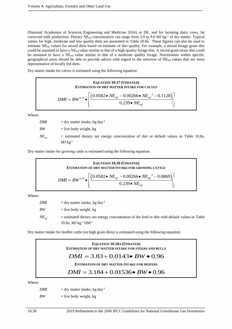
Volume 4: Agriculture, Forestry and Other Land Use
10.30 2019 Refinement to the 2006 IPCC Guidelines for National Greenhouse Gas Inventories
(National Academies of Sciences Engineering and Medicine 2016) or DE, and for lactating dairy cows, fat
corrected milk production. Dietary NEmf concentration can range from 3.0 to 9.0 MJ kg-1 of dry matter. Typical
values for high, moderate and low quality diets are presented in Table 10.8a. These figures can also be used to
estimate NEmf values for mixed diets based on estimate of diet quality. For example, a mixed forage-grain diet
could be assumed to have a NEmf value similar to that of a high-quality forage diet. A mixed grain-straw diet could
be assumed to have a NEmf value similar to that of a moderate quality forage. Nutritionists within specific
geographical areas should be able to provide advice with regard to the selection of NEmf values that are more
representative of locally fed diets.
Dry matter intake for calves is estimated using the following equation:
EQUATION 10.17 (UPDATED)
ESTIMATION OF DRY MATTER INTAKE FOR CALVES
2
0.750.0582 0.00266 0.1128
0.239
mf mf
mf
NE NEDMI BW
NE
Where:
DMI = dry matter intake, kg day-1
BW = live body weight, kg
mfNE = estimated dietary net energy concentration of diet or default values in Table 10.8a,
MJ kg-1
Dry matter intake for growing cattle is estimated using the following equation:
EQUATION 10.18 (UPDATED)
ESTIMATION OF DRY MATTER INTAKE FOR GROWING CATTLE
2
0.750.0582 0.00266 0.0869
0.239
mf mf
mf
NE NEDMI BW
NE
Where:
DMI = dry matter intake, kg day-1
BW = live body weight, kg
mfNE = estimated dietary net energy concentration of the feed or diet with default values in Table
10.8a, MJ kg-1 DM-1
Dry matter intake for feedlot cattle (on high grain diets) is estimated using the following equation:
EQUATION 10.18A (UPDATED)
ESTIMATION OF DRY MATTER INTAKE FOR STEERS AND BULLS
3.83 0.0143 0.96DMI BW
ESTIMATION OF DRY MATTER INTAKE FOR HEIFERS
3.184 0.01536 0.96DMI BW
Where:
DMI = dry matter intake, kg day-1
BW = live body weight, kg

Chapter 10:Emissions from Livestoch and Manure Management
2019 Refinement to the 2006 IPCC Guidelines for National Greenhouse Gas Inventories 10.31
For mature beef cows use the following values (National Academies of Sciences Engineering and Medicine 2016)
TABLE 10.8 (NEW)
DMI REQUIRED BY MATURE NON DAIRY COWS BASED ON FORAGE QUALITY
Forage type Digestibility (DE, %) Forage DMI capacity (kg/day), % of BW (kg)
Non-lactating Lactating
Low quality <52 1.8 2.2
Average quality 52-59 2.2 2.5
High quality >59 2.5 2.7
For lactating dairy cows the following equation can be used (Cornell Net Carbohydrate and Protein System
(CNCPS, Fox et al. 1992) as modified by Arnerdal (2005).
EQUATION 10.18B (UPDATED)
ESTIMATION OF DRY MATTER INTAKE FOR LACTATING DAIRY COWS
0.0185 0.305DMI BW FCM
Where:
DMI = dry matter intake, kg day-1
BW = live body weight, kg
FCM = Fat corrected milk kg day-1 3.5 percent [(0.4324 × kg of milk) + (16.216 x kg of fat)].
Equations 10.17, 10.18, 10.18A and 10.18B and values in Table 10.8 provide a good check to the main Tier 2
method to predict feed intake. They can be viewed as asking ‘what is an expected intake for a given diet quality?’
and in the case that countries do not have the data required to carry out a full estimate of gross energy use for their
catle herd, these equations could be used to independently predict DMI from BW, diet quality (NEmf or DE percent)
and milk production. In contrast, the main Tier 2 method predicts DMI based on how much feed must be consumed
to meet estimated energy requirements (i.e., NEm and NEg) and does not consider the biological capacity of the
animal to in fact consume the predicted quantity of feed. While the Tier 2 estimate of gross energy is the preferred
method, the simplified Tier 2 method can be used to confirm that DMI values derived from the main Tier 2 method
are biologically realistic. These estimates are also subject to the cross check that dry matter intake should be in
the order of 2 percent to 3 percent of the bodyweight of the mature or growing animals and up to 4 percent for
high yielding lactating dairy cattle.
TABLE 10.8A (UPDATED)
EXAMPLES OF NEMF CONTENT OF TYPICAL DIETS FED TO CATTLE FOR ESTIMATION OF DRY MATTER INTAKE
IN EQUATIONS 10.17 AND 10.18
Diet type NEmf (MJ (kg dry matter)-1)
High grain diet > 90% 7.5 - 8.5
High quality forage (e.g., vegetative legumes & grasses ) 6.5 - 7.5
Moderate quality forage (e.g., mid-season legume & grasses) 5.5 - 6.5
Low quality forage (e.g., straws, mature grasses) 3.5 - 5.5
Source: Estimates obtained from predictive models in NRC (1996), NEmf can also be estimated using the
equation: NEmf = REM x 18.45 x DE%
10.2.3 Uncertainty assessment
No refinement.

Volume 4: Agriculture, Forestry and Other Land Use
10.32 2019 Refinement to the 2006 IPCC Guidelines for National Greenhouse Gas Inventories
10.2.4 Characterisation for livestock without species:
Specific emission estimation methods
No refinement.
Some countries may have domesticated livestock for which there are currently no Tier 1 or Tier 2 emissions
estimating methods (e.g., wapiti, bison or emus). Good practice in estimating emissions from these livestock is to
first assess whether their emissions are likely to be significant enough to warrant characterising them and
developing country-specific emission factors. Volume 1, Chapter 4 (Methodological Choice and Identification of
Key Categories) presents guidance for assessing the significance of individual source categories within the national
inventory. Similar approaches can be used to assess the importance of subsource categories (i.e. species) within a
source category. If the emissions from a particular sub-species are determined to be significant, then country-
specific emission factors should be developed, and a characterisation should be performed to support the
development of the emission factors. Research into the estimation of emission levels from these non-characterized
species should be encouraged. The data and methods used to characterise the animals should be well documented.
As emissions estimation methods are not available for these animals, approximate emission factors based on ‘order
of magnitude calculations’ are appropriate for conducting the assessment of the significance of their emissions.
One approach for developing the approximate emission factors is to use the Tier 1 emissions factor for an animal
with a similar digestive system and to scale the emissions factor using the ratio of the weights of the animals raised
to the 0.75 power. The Tier 1 emission factors can be classified by digestive system as follows:
Ruminant animals: Cattle, Buffalo, Sheep, Goats, Camels;
Non-ruminant herbivores: Horses, Mules/Asses;
Poultry: Chickens, Ducks, Turkeys, Geese;
Non-poultry monogastric animals: Swine.
For example, an approximate enteric fermentation methane emissions factor for wapiti could be estimated from
the emissions factor for deer (also a ruminant animal) as follows:
Approximate emissions factor = [(wapiti weight) / (deer weight)]0.75 • deer emissions factor
Similarly, an approximate manure methane emissions factor could be estimated for emus using the Tier 1 emission
factor for ostriches. Approximate emission factors developed using this method can only be used to assess the
significance of the emissions from the animals, and are not considered sufficiently accurate for estimating
emissions as part of a national inventory.

Chapter 10:Emissions from Livestoch and Manure Management
2019 Refinement to the 2006 IPCC Guidelines for National Greenhouse Gas Inventories 10.33
10.3 METHANE EMISSIONS FROM ENTERIC
FERMENTATION
This section contains updated guidance
Methane is produced in herbivores as a by-product of enteric fermentation, a digestive process by which
carbohydrates are broken down by micro-organisms into simple molecules for absorption into the bloodstream.
The amount of methane released depends on the type of digestive tract, age, and weight of the animal, and the
quality and quantity of the feed consumed. Ruminant livestock (e.g., cattle, sheep) are major sources of methane
with moderate amounts produced from non-ruminant livestock (e.g., pigs, horses). The ruminant gut structure
fosters extensive enteric fermentation of their diet.
Digest ive system
The type of digestive system has a significant influence on the rate of methane emission. Ruminant livestock
have an expansive chamber known as the rumen, located at the fore-part of their digestive tract. The rumen
supports intensive microbial fermentation of the diet, which yields several nutritional advantages including the
capacity to digest cellulose (the major component of fiber). The main ruminant livestock are cattle, buffalo, goats,
sheep, deer and camelids. Non-ruminant livestock (horses, mules, asses) and monogastric livestock (swine) have
relatively lower methane emissions because much less methane-producing fermentation takes place in their
digestive systems.
Feed intake
Methane is produced by the fermentation of feed within the animal's digestive system. Generally, the higher the
feed intake, the higher the methane emission. Although, methane production is also affected by the composition
of the diet. Feed intake is positively related to animal size, growth rate, and production (e.g., milk production,
wool growth, or pregnancy).
To reflect the variation in emission rates among animal species, the population of animals should be divided into
subgroups, and an emission rate per animal is estimated for each subgroup. Types of population subgroups are
provided in Section 10.2 (Livestock and Feed Characterisation). The amount of methane emitted by a population
subgroup is calculated by multiplying the emission rate per animal by the number of animals within the subgroup.
Natural wild ruminants are not considered in the derivation of a country’s emission estimate. Emissions should
only be considered from animals under domestic management (e.g., farmed deer, elk, and buffalo).
10.3.1 Choice of method
It is good practice to choose the method for estimating methane emissions from enteric fermentation according to
the decision tree in Figure 10.2. The method for estimating methane emission from enteric fermentation requires
three basic steps:

Volume 4: Agriculture, Forestry and Other Land Use
10.34 2019 Refinement to the 2006 IPCC Guidelines for National Greenhouse Gas Inventories
Figure 10.2 (Updated) Decision Tree for CH4 Emissions from Enteric Fermentation
Start
Do you have
a country- specific Tier 3
methodology?
Do you have
population data by
productivity System?
Is enhanced livestock
characterization available?
Yes
Yes
No
No
Collect enhanced species
characterization data
for Tier 2 approach?
Estimate emissions for the
species using Tier 3 approach.
Estimate emissions for the
species using Tier 1 approach
Estimate emissions for the
species using Tier 1a approach.
Box 2: Tier 1a
Box 1: Tier 1
Box 4: Tier 3
No
Is enteric fermentation
a key category1 and is the
species significant2?
Yes
No
Yes
Estimate emissions for the
species using Tier 2 approach.
Box 3: Tier 2
Yes
Note:
1. See Volume 1 Chapter 4, ‘Methodological Choice and Identification of Key Categories’ (noting Section 4.1.2 on limited resources), for
discussion of key categories and use of decision trees.
2. As a rule of thumb, a livestock species would be significant if it accounts for 25-30% or more of emissions from the source category.
Step 1: Divide the livestock population into subgroups and characterize each subgroup as described in Section
10.2. It is recommended that national experts use annual averages estimated with consideration for the impact of
production cycles and seasonal influences on population numbers.
Step 2: Estimate emission factors for each subgroup in terms of kilograms of methane per animal per year.
Step 3: Multiply the subgroup emission factors by the subgroup populations to estimate subgroup emission,
and sum across the subgroups to estimate total emission.
These three steps can be performed at varying levels of detail and complexity. This chapter presents the following
three approaches:
Tier 1
A simplified approach that relies on default emission factors established in these guidelines that were either drawn
from the literature or calculated using regional data taken from the literature and derived using the Tier 2 method.

Chapter 10:Emissions from Livestoch and Manure Management
2019 Refinement to the 2006 IPCC Guidelines for National Greenhouse Gas Inventories 10.35
The Tier 1 method is likely to be suitable for most animal species in countries where enteric fermentation is not a
key source category, or where enhanced characterization data are not available. When approximate enteric
emissions are derived by extrapolation from main livestock categories they should be considered to be a Tier 1
method.
Tier 1a
An advanced Tier 1 method, applicable in particular to countries that have differentiated production systems with
coexistence of low and high productivity systems, or whose agricultural production systems are transitioning from
low to high productivity. Countries can consider the split in their production systems, yet still use default emission
factors, to customize their emission estimates based on populations of high and low productivity animals and
therefore track change in their emissions related to improved productivity.
Tier 2
A more complex approach that requires detailed country-specific data on gross energy intake and methane
conversion factors for specific livestock categories. The Tier 2 method should be used if enteric fermentation is a
key source category for the animal category that represents a large portion of the country’s total emissions.
Tier 3
Some countries for which livestock emissions are particularly important may wish to go beyond the Tier 2 method
and incorporate additional country-specific information in their estimates. This approach could employ the
development of sophisticated models that consider diet composition in detail, concentration of products arising
from ruminant fermentation, seasonal variation in animal population or feed quality and availability, and possible
mitigation strategies. Many of these estimates would be derived from direct experimental measurements.
Although countries are encouraged to go beyond the Tier 2 method presented below when data are available, these
more complex analyses are only briefly discussed here. A Tier 3 method should be subjected to a wide degree of
international peer review such as that which occurs in peer-reviewed publications to ensure that they improve the
accuracy and / or precision of estimates.
Countries with large populations of domesticated animal species for which there are no IPCC default emission
factors (e.g., llamas and alpacas) are encouraged to develop national methods that are similar to the Tier 2 method
and are based on well-documented research (if it is determined that emissions from these livestock are significant).
The approach is described in Section 10.2.4 under the heading ‘Characterisation for livestock without species-
specific emission estimation methods’ for more information.
Table 10.9 summarises the suggested approaches for the livestock emissions included in this inventory.
10.3.2 Choice of emission factors
Tier 1 Approach for methane emissions from Enteric Fermentation
This Tier 1 method is simplified so that only readily-available animal population data are needed to estimate
emissions. Default emission factors are presented for each of the recommended population subgroups. Each step
is discussed in turn.
Step 1: Animal population and productiv ity system
The animal population data should be obtained using the approach described in Section 10.2.
Step 2: Emiss ion factors
The purpose of this step is to select emission factors that are most appropriate for the country's livestock
characteristics. Default emission factors for enteric fermentation have been drawn from previous studies, and are
organised by region and by productivity system for ease of use.
The data used to estimate the default emission factors for enteric fermentation are presented in Annex 10A.1.

Volume 4: Agriculture, Forestry and Other Land Use
10.36 2019 Refinement to the 2006 IPCC Guidelines for National Greenhouse Gas Inventories
TABLE 10.9 (UPDATED)
SUGGESTED EMISSIONS INVENTORY METHODS FOR ENTERIC FERMENTATION
Livestock Suggested emissions inventory methods
Dairy Cow Tier 2a/Tier 3
Other Cattle Tier 2a/Tier 3
Buffalo Tier 1/Tier 2
Sheep Tier 1/Tier 2
Goats Tier 1/Tier 2
Camels Tier 1
Horses Tier 1
Mules and Asses Tier 1
Swine Tier 1
Poultry Not developed
Other (e.g., Llamas,
Alpacas, Deer, Ostrich) Tier 1
a The Tier 2 method is recommended for countries with large livestock populations. Implementing the
Tier 2 method for additional livestock subgroups may be desirable when the category emissions are a
large portion of total methane emissions for the country.
Table 10.10 shows the enteric fermentation emission factors for each of the animal species except cattle and
buffalo. As shown in the table, emission factors for sheep, goats and swine vary for low and high productivity
systems and it is important to consider that these conditions may exist within individual countries. The differences
in the emission factors are driven by differences in feed intake (as related to animal size) and feed characteristic
assumptions. Table 10.11 presents the enteric fermentation emission factors for cattle and buffaloes, accordingly.
A range of emission factors is shown for typical regional conditions.
Animal size and milk production are important determinants of emission rates for dairy cows. Relatively smaller
dairy cows with low levels of production are found in Asia, Africa, and the Indian subcontinent. Relatively larger
dairy cows with high levels of production are found in North America, Western Europe and several countries of
Latin America.
Animal size and population structure and production systems implemented are important determinants of emission
rates for other cattle. Relatively smaller other cattle are found in Asia, Africa, and the Indian subcontinent. Also,
many of the other cattle in these regions are young. Other cattle in North America, Western Europe and Oceania
are larger, and young cattle constitute a smaller portion of the population.
For countries with highly differentiated agricultural systems in which there is a coexistence of low and high
productivity systems or whose agricultural systems are transitioning from local low input productivity systems to
higher productivity systems and do not have the information necessary for implementing Tier 2 method, the use
of the diversification of emission factors given for an animal category provides an alternative or intermediary
option. This approach can reflect changes in activity data and productivity with time, whereas the Tier 1a approach
only take into account changes in the number of animals in a country.
To select emission factors from Tables 10.10 and 10.11 identify the region most applicable to the country being
evaluated. Scrutinise the tabulations in Annex 10A.1 to ensure that the underlying animal characteristics such as
weight, growth rate and milk production used to develop the emission factors are similar to the conditions in the
country. The data collected on the average annual milk production by dairy cows should be used to help select a
dairy cow emission factor. If necessary, interpolate between dairy cow emission factors shown in the table using
the data collected on average annual milk production per head.
Note that using the same Tier 1 emission factors for the inventories of successive years means that no allowance
is being made for changing livestock productivity, such as increasing milk productivity or trend in live weight. If
it is important to capture the trend in methane emission that results from a trend in livestock productivity, then
livestock emissions can become a key source category based on trend and a Tier 2 calculation should be used.

Chapter 10:Emissions from Livestoch and Manure Management
2019 Refinement to the 2006 IPCC Guidelines for National Greenhouse Gas Inventories 10.37
TABLE 10.10 (UPDATED)2,3
ENTERIC FERMENTATION EMISSION FACTORS FOR TIER 1 METHOD (KG CH4 HEAD-1 YR-1)
Livestock High Productivity
Systems1
Low Productivity
Systems Liveweight7
Sheep 9 5 40 kg – high productivity systems6
31 kg – low productivity systems
Swine 1.5 1 72 kg - high productivity systems6
52 kg - low productivity systems
Goats 9 5 50 kg – high productivity systems5
28 kg – low productivity systems
Horses 18 550 kg
Camels 46 570 kg
Mules and Asses 10 245 kg
Deer 20 120 kg
Ostrich4 5 120 kg
Poultry Insufficient data for calculation
Llamas and Alpacas 8 65 kg
Other (e.g., bison) To be determined
All estimates have an uncertainty of +30-50%.
Sources:
Emission factors camels from Gibbs & Johnson (1993). Alpacas from Pinares-Patino et al. (2003); Deer from Clark et al. (2003); Sheep (High productivity systems) derived from Swainson et al. (2016). Sources and assumptions to calculate goats EFs are detailed in Annex
10B.3. Emission factors for other livestock from Crutzen et al. (1986),
1 For the application of the simple Tier 1, for all regions other than North America, Europe and Oceania the Tier 1 default values are the
low productivity EFs. 2 One approach for developing the approximate emission factors is to use the Tier 1 emissions factor for an animal with a similar
digestive system and to scale the emissions factor using the ratio of the weights of the animals raised to the 0.75 power. Liveweight values have been included for this purpose. Emission factors should be derived on the basis of characteristics of the livestock and feed of
the animals and compilers should not base their decision of an emission factor entirely on regional characteristics.
3 The enteric fermentation emission factor shall be applied for the whole livestock population including non-mature animals.
4 CH4 EF for ostrich was calculated based on Frei et al. (2015) and Danish NIR (Nielsen et al. 2018). 5 Sources and assumptions to adjust weight of goats for low- and high-productivity systems are detailed in Annex 10B.3.
6 The values of swine weight for low and high productivity systems were obtained from FAO GLEAM databases (FAO 2017). More detailed data on swine weight are reported in Annex 10A.2 (in Table 10A.5). Crutzen et al. (1986) did not report weights for swine.
Regional Tier 2 calculations for swine have been carried out by the FAO GLEAM research group, countries could consult these values
for consistency with their production systems for refinement to their emission factors. 7 If a country-specific liveweight of animal category is different from those reported in Table 10.10, an inventory-compiler may use the
approach presented in section 10.2.4 of the current chapter.
It is recommended to continue to use Tier 1 emission factor uncertainty ranges as defined in Section 10.3.4 of the 2006 IPCC Guidelines.
Step 3: Tota l emiss ion
To estimate total emission, the selected emission factors are multiplied by the associated animal population
(Equation 10.19) and summed (Equation 10.20):

Volume 4: Agriculture, Forestry and Other Land Use
10.38 2019 Refinement to the 2006 IPCC Guidelines for National Greenhouse Gas Inventories
EQUATION 10.19 (UPDATED)
ENTERIC FERMENTATION EMISSIONS FROM A LIVESTOCK CATEGORY (TIER 1)
,
, 610
T P
T P T P
NE EF
Where:
TE = methane emissions from Enteric Fermentation in animal category T, Gg CH4 yr-1
, T PEF = emission factor for the defined livestock population T and the productivity system P, in kg
CH4 head-1 yr-1
, T PN = the number of head of livestock species / category T in the country classified as
productivity system P.
T = species/category of livestock
P = productivity system, either high or low productivity for use in advanced Tier 1a – omitted
if using Tier 1 approach
EQUATION 10.20 (UPDATED)
TOTAL EMISSIONS FROM LIVESTOCK ENTERIC FERMENTATION (TIER 1)
4 ,
,
Enteric i P
i P
Total CH E
Where:
4 EntericTotal CH = total methane emissions from Enteric Fermentation, Gg CH4 yr-1
,i PE = is the emissions for the ith livestock categories and subcategories based on production
systems (P)
Tier 1 method entails multiplying the total number of livestock population and CH4 emission factor for each
category of livestock (Table 10.10 or Table 10.11). Tier 1a method relies on number of livestock population in
each productivity systems (i.e., low-productivity systems and high-productivity systems) and CH4 emission factor
for each category of livestock developed per head of animal kept in the specified productivity system (Table 10.10
or Table 10.11).

Chapter 10:Emissions from Livestoch and Manure Management
2019 Refinement to the 2006 IPCC Guidelines for National Greenhouse Gas Inventories 10.39
TABLE 10.11 (UPDATED)
TIER 1 AND TIER 1A ENTERIC FERMENTATION EMISSION FACTORS FOR CATTLE AND BUFFALO1
Regional characteristics8 Animal category
Tier 1 and Tier
1a Emission
Factor 2,3
(kg CH4 head-1
yr-1)
Comments7
North America
Cattle: Highly productive
commercialized dairy sector
feeding high quality forage and
grain. Separate beef cow herd,
primarily grazing with feed
supplements seasonally. Fast-
growing beef steers/heifers finished
in feedlots on grain. Dairy cows are
a small part of the population.
There are no buffalo herds, but
American bison may be raised.
Dairy Cattle 138 Average milk production of
10,250 kg head-1 yr-1.
Other cattle 64
Includes mature males, multi-
purpose mature females, calves,
growing steers/heifers, and
feedlot cattle.
Western Europe
Cattle: Highly productive
commercialised dairy sector
feeding high quality forage and
grain. Dairy cows also used for
beef calf production. Very small
dedicated beef cow herd. Minor
amount of feedlot feeding with
grains.
Dairy Cattle 126 Average milk production of
7,410 kg head-1 yr-1.
Other cattle 52 Includes mature males, calves,
and growing steers/heifers.
Buffalo: Buffalo farming system is
exclusively intensive. The
concentrates are largely used only
during the lactation phase. Animals
are maintained in paddocks,
grazing practices are not
widespread.
Buffalo 78
Includes mature females, mature
males, growing animals and
calves.
Eastern Europe
Cattle: Commercialised dairy
sector feeding based on forages and
gains. Separate beef cow herd,
primarily grazing. Minor amount of
feedlot feeding with grains.
Dairy cattle 93 Average milk production of
4,000 kg head-1 yr-1.
Other cattle 58
Includes mature males, mature
females, growing and
replacement animals, and calves.
Buffalo: Commercialized buffalo
sector feeding primarily with
roughages. Buffaloes are managed
according to their categories.
Animals are maintained paddock
and tied up during the winter, in
summer they are allowed to graze
Buffalo 68
Includes mature females, mature
males, growing animals and
calves.

Volume 4: Agriculture, Forestry and Other Land Use
10.40 2019 Refinement to the 2006 IPCC Guidelines for National Greenhouse Gas Inventories
TABLE 10.11 (UPDATED) (CONTINUED)
TIER 1 AND TIER 1A ENTERIC FERMENTATION EMISSION FACTORS FOR CATTLE AND BUFFALO1
Regional characteristics8 Animal category
Tier 1 and Tier
1a Emission
Factor 2,3
(kg CH4 head-1
yr-1)
Comments7
Oceania4
Cattle: Commercialised dairy
sector based on grazing. Separate
beef cow herd, primarily grazing
rangelands5 and hill country of
widely varying quality. Growing
amount of feedlot feeding with
grains. Dairy cows are a small part
of the population. No Buffalo herd.
Dairy cattle 93 Average milk production of
4,400 kg head-1 yr-1.
Other cattle 63 Includes mature males, mature
females and young.
Latin America
Cattle: Commercialised dairy
sector based on grazing. Separate
beef cow herd grazing pastures and
rangelands. Minor amount of
feedlot feeding with grains.
Growing non-dairy cattle comprise
a large portion of the population.
Dairy Cattle 87 Average milk production of
2,050 kg head-1 yr-1
High productivity
systems 103
Average milk production of
3,400 kg head-1 yr-1
Low productivity
systems 78
Average milk production of
1,250 kg head-1 yr-1
Other cattle 56
Includes mature females, mature
males, growing steers/heifers
and calves.
High productivity
systems 55
Low productivity
systems 58
Buffalo:Buffalo husbandry is based
on extensive systems in native or
cultivated pastures in lowlands and
uplands, most often without supply
of concentrated feed. Milk
production is based on pasture with
frequent supplementation of
roughage (sugar cane, silage, etc.),
with a predominance of one single
milking.
Buffalo 68
Includes mature females, mature
males, growing animals and
calves.

Chapter 10:Emissions from Livestoch and Manure Management
2019 Refinement to the 2006 IPCC Guidelines for National Greenhouse Gas Inventories 10.41
TABLE 10.11 (UPDATED) (CONTINUED)
TIER 1 AND TIER 1A ENTERIC FERMENTATION EMISSION FACTORS FOR CATTLE AND BUFFALO1
Regional characteristics8 Animal category
Tier 1 and Tier
1a Emission
Factor 2,3
(kg CH4 head-1
yr-1)
Comments7
Asia
Cattle: Commercialised dairy
sector is experienced fundamental
changes due to increasing number
of large farms with intensive
production system based on grains
and forage. Cattle kept in
traditional production systems are
multi-purpose, providing draft
power and some milk within
farming regions. Cattle of all types
are smaller than those found in
most other regions.
Dairy cattle 78 Average milk production of
3,200 kg head-1 yr-1
High productivity
systems 96
Average milk production of
5,000 kg head-1 yr-1
Low productivity
systems 71
Average milk production of
2,600 kg head-1 yr-1
Other cattle 54
Includes mature males, mature
females, growing and
replacement animals, and calves.
High productivity
systems 43
Low productivity
systems 56
Buffalo: Buffaloes are generally
swamp type. Buffaloes are raised
by smallholder farmers as source of
draft power. Animals are
commonly grazed in field and fed
on agriculture residual products.
Milk yield per cow is low.
Nevertheless, the dairy buffalo
breeding is rapidly developing in
countryside of Asia.
Buffalo 76
Includes breeding and working
bulls, growing animals and
calves
Africa6
Cattle: Commercialised dairy
sector based on grazing with low
production per cow. Most cattle
are multi-purpose, providing draft
power and some milk within
farming regions. Some cattle graze
over very large areas. Cattle are
smaller than those found in most
other regions.
Dairy cattle 76 Average milk production of
1,300 kg head-1 yr-1
High productivity
systems 86
Average milk production of
2,200 kg head-1 yr-1
Low productivity
systems 66
Average milk production of 500
kg head-1 yr-1
Other cattle 52
Includes mature males, multi-
purpose mature females,
growing and replacement
animals, and calves.
High productivity
systems 60
Low productivity
systems 48
Buffalo: Small-scale buffalo sector
well-integrated with cropland.
Animals are raised for multi-
purpose. Feeding primarily depends
on roughages and crop-residues.
Minor commercial dairy buffalo
farms feeding with concentrate feed
mixture.
Buffalo 81
Includes breeding and working
bulls, growing animals and
calves

Volume 4: Agriculture, Forestry and Other Land Use
10.42 2019 Refinement to the 2006 IPCC Guidelines for National Greenhouse Gas Inventories
TABLE 10.11 (UPDATED) (CONTINUED)
TIER 1 AND TIER 1A ENTERIC FERMENTATION EMISSION FACTORS FOR CATTLE AND BUFFALO1
Regional characteristics8 Animal category
Tier 1 and Tier
1a Emission
Factor 2,3
(kg CH4 head-1
yr-1)
Comments7
Middle East
Cattle: Majority of cattle
population is still kept by small
holders in the traditional production
systems. The animals are fed
primarily by crop residues and are
grazed. Most animals are dual-
purpose. In contrast to the small-
scale farms, commercial dairy
sector is generally intensive, mainly
based on compound feed and
grains.
Dairy cattle 76 Average milk production of
2,500 kg head-1 yr-1
High productivity
systems 94
Average milk production of
3,900 kg head-1 yr-1
Low productivity
systems 62
Average milk production of
1,300 kg head-1 yr-1
Other cattle 60
Includes mature males, multi-
purpose mature females,
growing and replacement
animals, and calves.
High productivity
systems 61
Low productivity
systems 55
Buffalo: Buffalo farming system
primarily based on smallholders
rearing animals for meat, milk and
draught. Animals obtain their
feeding by grazing. Minor
commercialized buffalo sector
feeding forage and concentrate
supplemented feed.
Buffalo 67
Includes breeding and working
bulls, growing animals and
calves
Indian Subcontinent
Cattle: Commercialised dairy sector
based on crop by-product feeding
with low production per cow. Most
bullocks provide draft power and
cows provide some milk in farming
regions. Cattle in this region are the
smallest compared to cattle found in
all other regions.
Dairy cattle 73 Average milk production of
1,900 kg head-1 yr-1
High productivity
systems 70
Average milk production of
2,600 kg head-1 yr-1
Low productivity
systems 74
Average milk production of
1,700 kg head-1 yr-1
Other Cattle
46
Includes mature males, multi-
purpose mature females,
growing and replacement
animals, and calves.
High productivity
systems 41
Low productivity
systems 47
Buffalo: Smallholder buffalo sector
feeding poor quality roughages and
crop-residues. Buffaloes are
primarily free grazing. Concentrates
are fed to dairy animals during last
months of pregnancy. Dairy and
meat production are intimately
related. Animals are used as draft
power. Minor commercialized
buffalo sector providing animals
with balanced ration.
Buffalo 85
Includes breeding and working
bulls, growing animals and
calves

Chapter 10:Emissions from Livestoch and Manure Management
2019 Refinement to the 2006 IPCC Guidelines for National Greenhouse Gas Inventories 10.43
TABLE 10.11 (UPDATED) (CONTINUED)
TIER 1 AND TIER 1A ENTERIC FERMENTATION EMISSION FACTORS FOR CATTLE AND BUFFALO1
1 Emission factors should be derived on the basis of the characteristics of the cattle and feed of the animals and compilers should not base
their decision of an emission factor entirely on regional characteristics.
2 The values represent averages within region. Existing values were derived using Tier 2 method and the data in Tables 10A.1–10A.4.
Data on a livestock population mix corresponding to low- and high-productivity systems were used. 3 Uncertainty values from the previous guidelines were validated during the development of the emission factors using a Monte Carlo
analysis in the 2019 Refinement, based on data compiled during the emission factor development process. It is recommended to continue
to use Tier 1 emission factor uncertainty ranges as defined in Section 10.3.4 of the 2006 IPCC Guidelines. 4 All data are weighted values, representative of Australia and New Zealand. For Pacific Island nations, refer to Asia values. Island
nations from Oceania may wish to use a Tier 1a method. In this case, they could used values from Asia, or low productivity systems from
Asia and high the Tier 1a emission factor from Oceania, whichever is more representative of their production systems. 5 Rangelands are defined as land primarily covered by woodlands, shrublands, grasslands and savannas, as well as introduced plant
species that are naturalised (Grice et al. 2008).
6 North African countries may wish to use values derived for the Middle East if productions systems are more similar. 7 Buffalo mature females livestock sub-category includes lactating (dairy) mature females.
8 Sources: Cattle of Asia: IPCC (2006); Ma et al. (2007); Ma et al. (2012); FAO et al. (2014) . Cattle of Middle East: Kamalzadeh et al. (2008); Karakok (2007); Yilmaz et al. (2012); Yilmaz & Wilson (2012); FAO et al. (2014). Buffalo of Western Europe: Borghese (2013);
Neglia et al. (2014); Sabia et al. (2015). Buffalo of Eastern Europe: FAO (2005). Buffalo of Latin America: Bernardes (2007). Buffalo of
Asia: Cruz (2007); Yang et al. (2007). Buffalo of Africa: Habeeb et al. (2016); Radwan (2016); Ali et al. (2009); Hassan & Abdel-Raheem (2013); Ibrahim (2012); Soliman (2009). Ali et al. (2009). Buffalo of Middle East: Azary et al. (2007); Soysal (2013); Dezfuli et al.
(2011); Hossein-zadeh et al. (2012); Soysal et al. (2007); Naserian & Saremi (2007); Ermetin (2017). Dezfuli et al. (2011). Buffalo of
Indian subcontinent: Ranjhan (2007); Anjum et al. (2012); Khan et al. (2008); Khadda et al. (2017); Ahirwar (2010); Khan et al. (2007);
Chawla et al. (2009)
Tier 2 Approach for methane emissions from Enteric Fermentation
The Tier 2 method is applied to more disaggregated livestock population categories and used to calculate emission
factors, as opposed to default values. The key considerations for the Tier 2 method are the development of
emission factors and the collection of detailed activity data.
Step 1: Livestock populat ion
The animal population data and related activity data should be obtained following the approach described in
Section 10.2.
Step 2: Emiss ion factors
When the Tier 2 method is used, emission factors are estimated for each animal category using the detailed data
developed in Step 1.
The emission factors for each category of livestock are estimated based on the gross energy intake and methane
conversion factor for the category. The gross energy intake data should be obtained using the approach described
in Section 10.2. The following two sub-steps need to be completed to calculate the emission factor under the Tier
2 method:
1. Obtaining the methane conversion factor (Y m)
The extent to which feed energy is converted to CH4 depends on several interacting feed and animal factors and
that rate of conversion is embodied in the methane conversion factor (Ym), defined as the percentage of gross
energy intake converted to methane.
There are a wide variety of factors that influence methane conversion rates and due to national circumstances
related to breeds, genetic pools as well as particularities of feed and herd interactions, the Ym factors may vary
from region to region. Considering interactions between feed (type and quality) and animals (breed and genetics),
it is good practice for countries to derive their own Ym values considering their herds and their typical feed
characteristics.
Nonetheless, numerous empirical studies demonstrate the statistical significance of improved feed quality on
methane emission rates and biochemical modelling exhibits the biochemical processes that impact methane
production with the introduction of improved feeds and concentrates to ruminant diets (Mills et al. 2001; Mills
et al. 2003; Ellis et al. 2006; Ellis et al. 2007; Ellis et al. 2009; Ellis et al. 2010; Alemu et al. 2011; Bannink et
al. 2011; Ellis et al. 2014; Escobar-Bahamondes et al. 2016; Kebreab et al. 2016). When country specific Ym
factors for cattle and buffalo are unavailable, the values provided in Table 10.12 can be used. These estimates are
a guide based on the general feed characteristics and production practices found in many countries. It is good
practice for compilers to justify their choice of Ym factors based on detailed feed data and research.

Volume 4: Agriculture, Forestry and Other Land Use
10.44 2019 Refinement to the 2006 IPCC Guidelines for National Greenhouse Gas Inventories
In Table 10.12, the Ym of dairy cows is linked to annual milk production levels and to feed quantity and quality.
The lowest Ym value is associated with highest producing dairy cattle that are fed diets of greater than 70 percent
digestibility, and that have percentage of NDF in DMI of less than 35 percent. These diets may be further
supplemented with additives or supplements that impact feed efficiency. In cases where countries are achieving
high production on high quality silage diets that have digestibility greater than 70 percent but also NDF greater
than 35 percent of DMI, compilers should use Ym values that are midway between the high production and the
mid-range productivity Ym values (6.0 percent GEI).
Diets with digestible fractions that range from 63 to 70 percent and NDF greater than 37 percent DMI, consisting
of good quality forages, silages and some grains and have associated milk production between 5000 to 8500 kg
year-1, are advised to use Ym values of 6.3 percent GEI. For low production dairy systems with feed digestibility
less than 62 percent and NDF fractions greater than 38 percent, the Ym factor from the 2006 IPCC Guidelines
(6.5) has been maintained as there is a paucity of reliable globally representative data that could be used to revise
that value. In cases where dairy cattle are strictly grazed on low quality forage diets, compilers should use the
non-dairy low quality forage value of 7.0 percent GEI.
It is important for inventory compilers to base their decision to select the Ym on a thorough understanding of
national feeding systems. In the case of dairy cows, milk production is presented as a proxy for feed quality and
Ym values in Table 10.12 represent the relationship between feed quality and methane yield. It is possible for a
country’s national herd, or for parts of the national herd, to have production levels that are inconsistent with the
feed quality bounds that are defined by the categories in Table 10.12. In these cases, it is good practice to develop
their own country-specific Ym factors, and they should also use their information on animal diets to validate their
choice of Ym against methane yield equations recommended in Niu et al. (2018).
With the non-dairy animal category, the non-feedlot diets can be differentiated between forage based diets for
which the Ym value of 7.0 should be used, and mixed concentrate diets or high quality forage diets for which
compilers should use the value of 6.3. Reliable estimates for grazing cattle on very poor quality diets are not
available, and due to the lack of data, the value of 7.0 is recommended. Countries that have large cattle herds
consuming these types of diets are encouraged to develop country-specific values and research efforts should
focus on providing more data on these cattle herds.
Emissions from feedlot animals are influenced by the type of grain fed to the animals during the finishing stage,
the lowest value of 3.0 can be used when steam-flaked corn is fed at rates greater than 90 percent of the diet in
combination with ionophores. Low forage diets of less than 15 percent that incorporate other grains are
recommended to use the value of 4.0.
A methane conversion rate of zero is assumed for all juveniles consuming only milk (i.e., milk-fed lambs and
calves). While some studies have demonstrated low level emissions from calves during the activation of their
rumens (Gerrits et al. 2014), the Ym for the addition of small quantities of emission from unweaned calves does
not significantly influence emission factors. For weaned animals the Ym values indicated for the non-dairy animal
category are recommended.
Due to the importance of Ym in driving emissions, ongoing research is aimed at improving estimates for different
livestock and feed combinations. It is important to better understand the mechanisms involved in methanogenesis
with a view to designing emission abatement strategies, as well as to identify different values for Ym according
to animal husbandry practices.
Significant improvement are needed for grazing animals in general, but in particular for low producing dairy cattle
on diverse diets and grazing animals on low quality forages particularly in tropical regions as the available data
are currently very sparse.
Regional, national and global estimates of enteric methane generation rely on small-scale determinations both of
Ym and of the influence of feed and animal properties upon Ym. Traditional methods for measuring Ym include
the use of respiration calorimeters and head enclosures for housing individual animals (Johnson & Johnson 1995).
A tracer technique using SF6 enables methane emissions from individual animals to be estimated under both
housed or grazing conditions (Johnson et al. 1994). Hammond et al. (2015) present an in-depth review of the
advantages and limitations of methane measurement techniques used to determine Ym values.

Chapter 10:Emissions from Livestoch and Manure Management
2019 Refinement to the 2006 IPCC Guidelines for National Greenhouse Gas Inventories 10.45
TABLE 10.12 (UPDATED)6
CATTLE/BUFFALO METHANE CONVERSION FACTORS (YM )
Livestock
category Description
Feed quality
Digestibility (DE %)
and Neutral
Detergent Fibre
(NDF, % DMI)
MY,
g CH4 kg DMI-1 Ym
3
1,4Dairy cows
and Buffalo
High-producing cows5 (>8500
kg/head/yr-1)
DE ≥ 70
NDF ≤ 35 19.0 5.7
High-producing cows5 (>8500
kg/head/yr-1)
DE ≥ 70
NDF ≥ 35
20.0
6.0
Medium producing cows
(5000 – 8500 kg yr-1)
DE 63-70
NDF > 37 21.0 6.3
Low producing cows
(<5000 kg yr-1)
DE ≤ 62
NDF >38 21.4 6.5
2Non dairy and
multi-purpose
Cattle and
Buffalo
> 75 % forage DE ≤ 62 23.3 7.0
Rations of >75% high quality
forage and/or mixed rations,
forage of between 15 and 75%
the total ration mixed with
grain, and/or silage.
DE 62–71 21.0 6.3
Feedlot (all other grains, 0-
15% forage) DE ≥ 72 13.6 4.0
Feedlot (steam-flaked corn,
ionophore supplement - 0-10%
forage)
DE > 75 10.0 3.0
1Expert opinion of IPCC Panel in consideration of Appuhamy et al. (2016); Jayasundara et al. (2016) Hellwing et al. (2017) and Niu et
al. (2018) 2 Sources: Boadi and Wittenberg (2002); Pinares-Patiño et al. (2003); Boadi et al. (2004); Beauchemin and McGinn (2005);
Beauchemin and McGinn (2006a); Beauchemin and McGinn (2006b); Chaves et al. (2006); Jordan et al. (2006a); Jordan et al. (2006b);
Beauchemin et al. (2007); Hegarty et al. (2007); Hart et al. (2009); McGinn et al. (2009); Mc Geough et al. (2010a); Mc Geough et al. (2010b); Doreau et al. (2011); Hales et al. (2012); Kennedy and Charmley (2012); Staerfl et al. (2012); Chung et al. (2013); Hünerberg
et al. (2013); Fiorentini et al. (2014); Hales et al. (2014); Hales et al. (2015); Troy et al. (2015); Nascimento et al. (2016); Vyas et al.
(2016a); Vyas et al. (2016b); Baron et al. (2017); Hales et al. (2017). 3 Uncertainty values are ± 20% based on published standard deviations from Niu et al. (2018) and data compilations for non dairy cattle
as described in Annex B.2.
4 Ym cited for dairy cattle are for lactating dairy cows. For dairy cattle during their dry phase, in high and medium production systems, the non-dairy high quality forage value (6.3) should be selected and for low production systems with >75% low quality forage the value
of (7.0) should be selected.
5 The lowest Ym factors for high producing cows refers to feeding situations in which additives or supplements may be used in production that stimulate feed use efficiency and/or milk production. The Ym values given here do not yet account for any potential
reducing effect of additives or supplements on Ym.
6 For details on the development of these values, refer to Annex 10B.2
Table 10.13 proposes a common Ym value for all sheep irrespective of feed quality values. This value is based on
the mean value of raw data from New Zealand collated between 2009 and 2015 (Swainson et al. 2016). Data were
derived from respiration chamber measurements where intake was accurately measured and covered a range of
diet qualities. These replace values in the 2006 IPCC Guidelines which were based on indirect measurements
using the sulphur hexafluoride tracer technique where dry matter intake was generally estimated in grazing
animals (Ulyatt et al. 2002a; Ulyatt et al. 2002b; Ulyatt et al. 2005). The mean value of 6.7 percent is most
appropriate for situations where average dry matter intake per day is between 0.6 and 0.8 kg/day with a value of
7.0 percent being more appropriate where average intake is <0.6kg/day, and a value of 6.5 percent being more
appropriate where average intakes are >0.8kg day-1. Table 10.13 also includes a Ym value for goats (2006 IPCC
Guidelines did not propose any specific value for goats). This value is based on the analysis of 65 studies that
calculated in-vivo enteric CH4 production from a varied sample of countries and goat breeds (sources and
assumptions are explained in Annex 10B.3.).

Volume 4: Agriculture, Forestry and Other Land Use
10.46 2019 Refinement to the 2006 IPCC Guidelines for National Greenhouse Gas Inventories
TABLE 10.13 (UPDATED)
SHEEP AND GOATS CH4 CONVERSION FACTORS (YM)
Category Ym 1
Sheep 6.7% + 0.9
Goats 5.5% + 1.0
Sources and assumptions to calculate the Ym for goats are detailed in Annex 10B.3.
1 The ± values are the the standard deviation of the mean of the Ym..
Note that in some cases, CH4 conversion factors may not exist for specific livestock types. In these instances, CH4
conversion factors from the reported livestock that most closely resembles those livestock types can be reported.
For examples, CH4 conversion factors for other cattle or buffalo could be applied to estimate an emission factor
for camels.
2. Emission factor development
Using the energy balance Tier 2 approach an emission factor for each animal category should be developed
following Equation 10.21:
EQUATION 10.21
METHANE EMISSION FACTORS FOR ENTERIC FERMENTATION FROM A LIVESTOCK CATEGORY
365100
55.65
mYGE
EF
Where:
EF = emission factor, kg CH4 head-1 yr-1
GE = gross energy intake, MJ head-1 day-1
mY = methane conversion factor, per cent of gross energy in feed converted to methane
The factor 55.65 (MJ/kg CH4) is the energy content of methane
In cases in which the inventory compiler has used the simplified Tier 2 the emission factors should be calculated
following equation 10.21a:
EQUATION 10.21A (NEW)
METHANE EMISSION FACTORS FOR ENTERIC FERMENTATION FROM A LIVESTOCK CATEGORY
3651000
MYEF DMI
Where:
EF = emission factor, kg CH4 head-1 yr-1
DMI = kg DMI day-1
MY = Methane yield, kg CH4 kg DMI-1 (Table 10.12)
365 = days per year
1000 = conversion from g CH4 to kg CH4
These emission factor equations assume that the emission factors are being developed for an animal category for
an entire year (365 days). While a full year emission factor is typically used, in some circumstances the animal
category may be defined for a shorter period (e.g., for the wet season of the year or for a 150-day feedlot feeding

Chapter 10:Emissions from Livestoch and Manure Management
2019 Refinement to the 2006 IPCC Guidelines for National Greenhouse Gas Inventories 10.47
period). In this case, the emission factor would be estimated for the specific period (e.g., the wet season) and the
365 days would be replaced by the number of days in the period. The definition of the period to which the emission
factor applies is described in Section 10.2, defined according the the enhanced livestock characterisation that is
used in calculation methodology.
Step 3: Tota l emiss ions
To estimate total emissions, the selected emission factors are multiplied by the associated animal population and
summed. As described above under Tier 1, the emissions estimates should be reported in gigagrams (Gg).
Potential for refinement of Tier 2 or development of a Tier 3 method to enteric
methane emission inventories
Increased accuracy and identification of causes of variation in emissions are at the heart of inventory purpose.
Improvements in country methodology, whether as components of current Tier 1 or 2 or if additional refinements
are implemented with Tier 3, are encouraged.
Tier 1 and Tier 2 enteric methane emissions factors and estimation procedures are driven by first estimating daily
and annual gross energy consumption by individual animals within an inventory class which are then multiplied
by an estimate of CH4 loss per unit of feed (Ym). There is considerable room for improvement in Tier 2 prediction
of both feed intake and in Ym. Factors potentially impacting feed requirements and/or consumption may include:
depression in digestibility with increasing levels of consumption or due to rumen acidification, feed preparation
or diet composition putting limits to feed intake;
breed or genotype variation in maintenance requirement; and
heat and cold stress effects on feed intake and maintenance requirements.
Likewise, a host of interacting factors cause variation in the rumen microbiome and its fermentation profile, and
hence in hydrogen production which delivers the main substrate for methanogens. These factors lead to variation
in Ym that may include:
variation in feed digestibility (DE);
breed or genotype variation;
level of feed intake;
chemical composition of feed;
kinetics of particle and fluid passage and of digestion, rumen volume, rumen fermentation profile; and
other factors (such as secondary plant compounds, additives and other products) affecting the rumen microbiome.
The values in Table 10.12 capture some aspects of these factors as they are broadly related to feed quality and
animal productivity, however these estimates can be improved for country-specific cirucumstances using higher
Tier methods. Accurate estimation of diet DE is singularly important in the estimation of feed intake and enteric
methane emission, as previously emphasized. A change of 10 percent in DE will be magnified to a change in CH4
emissions ranging from 12 to 20 percent depending on the dietary circumstances for which calculations are made.
The depression in DE with increasing daily amounts of feed consumed (increasing rates of passage) is not
inherently considered with Tier 2 and this neglect could underestimate feed intakes of high producing dairy cows
consuming mixtures of concentrates and forages as is common in the North America and Europe, and hence
underestimate methane emission. The balance between both effects (i.e. a reduction of feed digestibility and of
Ym) determines the net effect on methane emission which may vary with dietary circumstances. More complex
models may be developed as Tier 3 to capture the intricacies of such effects.
There have been many attempts to refine estimates of Ym. Several researchers have developed models which relate
the chemical composition of the diet consumed, or in more detail, the composition of digested carbohydrate and
other chemical components to Ym. These models typically predict diet particle and chemical component rates of
passage and digestion in each enteric compartment at varying intake and the resulting H2 balance, volatile fatty
acids, and microbial and CH4 yields. These approaches have generated Ym values that are consistent with direct
measurements (Bannink et al. 2011; Gregorini et al. 2013; Huhtanen et al. 2015; Dougherty et al. 2017). A
mechanistic model has been developed in the Netherlands that employs Tier 3 approach using a mechanistic model
(Bannink et al. 2011) to estimate CH4 yield from dairy cattle while the US use mechanistic models (Baldwin 1995;
Kebreab et al. 2008) to refine estimates of Ym for dairy and beef in different states within the US.

Volume 4: Agriculture, Forestry and Other Land Use
10.48 2019 Refinement to the 2006 IPCC Guidelines for National Greenhouse Gas Inventories
The literature contains many examples of the positive relationship of plant cell wall digestion to high acetic to
propionic end-product ratios, and to high CH4 yields. While fibrous carbohydrate digestion is the strongest
indicator of CH4 yield, the CH4 per digested fiber is not constant and enteric fermentation of similar fibrous feeds
can result in different Ym values. For example, grass silage made from grass cut at different stages of maturity
resulted in strongly different carbohydrate and protein composition, resulting in Ym values varying from 5.5 to
6.9 percent with increased maturity and intake (Warner et al. 2017). Exchange of carbohydrates may also lead to
a lower Ym as demonstrated in studies where an increased dietary starch content through a higher proportion of
corn silage (Hassanat et al. 2013; Benchaar et al. 2014) or through a higher proportion of starch containing
concentrates (Aguerre et al. 2011). Prerequisite for the use of more complex prediction models for broad country
inventories is that the data need to be provided to drive these more complex models of feed intake or Ym. It is
often difficult to define animal characteristics, productivity, and DE accurately for a livestock category in various
regions or various production systems in a country. Of particular importance is a good characterization of
roughages when they constitute a main part of the diet.
Ongoing global research, such as the use of direct methanogen inhibitors, 3-nitrooxypropanol (3-NOP), oxygen-
rich anions, fats and oils, ionophores or condensed tannins, and also genetic selection suggests a need to address
how they should be reflected in inventory compilation at Tier 2 or Tier 3. First, it is good practice that the
inventory reflect only those technologies or genotypes developed through selection conform to QA/QC principles
and have attracted a wide degree of international acceptance such as through peer-reviewed articles that include a
description of the technology, its efficacy and validation under field conditions. Second, it is good practice that
the inventory be accompanied by evidence of the uptake of the technology in agricultural practice, and apply it
only to emissions by those livestock where uptake can be validated. Mitigation measures and their representation
in inventory compilation should be supported by peer-reviewed publications.
Concluding, approaches to improve estimates of feed intake (i.e. of diet composition, DE and dietary GE content)
and Ym, and approaches to account for specific mitigation measures are to be encouraged, given due care on
limitations of the scope and on production circumstances where mitigation measures are applied and to which
predictive models or relationships must apply as well.
10.3.3 Choice of activity data
Livestock population data should be obtained using the approach described in Section 10.2. If using default enteric
emission factors for livestock (Tables 10.10, 10.11) to estimate enteric emissions, a basic (Tier 1) livestock
population characterisation is sufficient. To estimate enteric emissions from livestock using estimation of Gross
Energy Intake (Equations 10.21, or 10.21A), a Tier 2 characterisation is needed. As noted in Section 10.2, good
practice in characterising livestock populations is to conduct a single characterisation that will provide the activity
data for all emissions sources that depend on livestock population data.
10.3.4 Uncertainty assessment
Emission factors
No refinement.
Activ ity data
No refinement.
10.3.5 Completeness, Time series, Quality
Assurance/Quality Control and Reporting
No refinement.

Chapter 10:Emissions from Livestoch and Manure Management
2019 Refinement to the 2006 IPCC Guidelines for National Greenhouse Gas Inventories 10.49
10.4 METHANE EMISSIONS FROM MANURE
MANAGEMENT
This section describes how to estimate CH4 produced during the storage and treatment of manure, and from manure
deposited on pasture. The Tier 1 approach is based on default emission factors per unit volatile solid (VS) by animal
category and manure storage system.The Tier 2 is based on country-specific estimates of volatile solids and the impact
of interactions between manure management systems and animal categories on total CH4 emissions during excretion
and storage, including manure treatments such as the production of biogas.
The term ‘manure’ is used here collectively to include both dung and urine (i.e., the solids and the liquids) produced
by livestock. The emissions associated with the burning of dung for fuel are to be reported under Volume 2 (Energy),
or under Volume 5 (Waste) if burned without energy recovery. When manure is used in the production of biogas, the
emissions reported under the manure management category are those occurring on the farm site not resulting from
combustion. These include, on-farm storage of the digestion input materials - pre-digestion, leakage during the
digestion process and emissions from the storage and application of digestate to agricultural fields (included in Volume
4, Chapter 11, Emissions from Agricultural Soils). Emissions from biogas combustion during the production of
energy, whether on or off farm should be reported under Volume 2 “Energy”.
The decomposition of manure under anaerobic conditions (i.e., in the absence of oxygen), during storage and
treatment, produces CH4. These conditions occur most readily when large numbers of animals are managed in a
confined area (e.g., dairy farms, beef feedlots, and swine and poultry farms), and where manure is disposed of in
liquid-based systems. Emissions of CH4 related to manure handling and storage are reported under ‘Manure
Management.’
The main factors affecting CH4 emissions are the amount of manure produced and the portion of the manure that
decomposes anaerobically. The former depends on the rate of waste production per animal and the number of animals,
and the latter on how the manure is managed. When manure is stored or treated as a liquid (e.g., in lagoons, ponds,
tanks, or pits), it decomposes anaerobically and can produce a significant quantity of CH4. The temperature and the
retention time of the storage unit greatly affect the amount of methane produced. When manure is handled as a solid
(e.g., in stacks or piles) or when it is deposited on pastures and rangelands, it tends to decompose under more aerobic
conditions and less CH4 is produced.
10.4.1 Choice of method
There are three tiers to estimate CH4 emissions from livestock manure as shown in the 2006 IPCC guidelines.
To be consistent with consideration of differing productivity classes in section of enteric fermentation, a new tier 1
was developed. In some regions, particularly in developing countries, production systems can vary between high
productivity systems aimed at commercial food production and low productivity systems, largely serving local food
production. In this case countries may choose to use a Tier 1 method in which emission factors are defined for low
and high productivity systems based on the updated volatile solids and B0, and the values of volatile solids was aligned
with updated enteric fermentation section.
Guidance for determining which methods to use is shown in Figure 10.3 decision tree.
Tier 1
The Tier 1 method entails multiplying the total amount of VS excreted (from all livestock species/categories) in each
type of manure management system by an emission factor for that type of livestock category in the specified climate
zone and manure management system (see Equation 10.22). Emissions are summed over all manure management
systems and livestock category. The Tier 1 method is applied using IPCC default VS excretion factors (See Table
10.13a), default typical animal mass (see Table 10A.5), default CH4 Emission Factors (see Table 10.14), and default
animal waste management systems (AWMS). Animal waste management system (manure management systems) data
have been collected for regions and countries by the FAO and average manure fractions treated by different
management systems are presented in Annex 10A.2 Tables 10A.6 to 10A.9. As emissions from manure management
systems are highly temperature dependent, it is good practice to consider the climate zone associated with the locations

Volume 4: Agriculture, Forestry and Other Land Use
10.50 2019 Refinement to the 2006 IPCC Guidelines for National Greenhouse Gas Inventories
where manure is managed. Breakdowns of manure management systems by regional climate zone and production
system can be found in the supplemental data supplied with this Chapter, maintained on the IPCC document website,
identified as Supplemental Information Chapter 10, Volume IV, 2019 Refinement. Further finer-scale country-specific
data is also available from FAO GLEAM databases (FAO 2017).
An advanced Tier 1a method has been developed as an alternative for countries with differentiated agricultural systems
in which there is a coexistence of low and high productivity systems or whose agricultural systems are transitioning
from local low input productivity systems to higher productivity systems. In this case, where countries do not have
the information necessary for implementing Tier 2 systems, the use of the productivity based emission factors given
for an animal category provides an alternative or intermediary option. The advanced Tier 1a approach will provide an
estimate of the changes in both productivity and manure management that occur when a transition from lower
productivity systems to higher productivity systems occurs.
Tier 2
A more complex method for estimating CH4 emissions from manure management should be used where a particular
livestock species/category represents a significant share of a country’s emissions. This method requires detailed
information on animal characteristics and manure management practices, which is used to develop emission factors
specific to the conditions of the country.
The main differences between the Tier 1 and Tier 2 calculations is whether default information or country-specific
information is used in the calculation of emissions from manure management system. The Tier 2 system provides a
much wider group of options for estimating emissions from different manure management systems.
Tier 3
Some countries for which livestock emissions are particularly important may wish to go beyond the Tier 2 method
and develop models for country-specific methodologies or use measurement–based approaches to quantify emission
factors.
The method chosen will depend on data availability and national circumstances. Good practice in estimating CH4
emissions from manure management systems entails making every effort to use the Tier 2 method, including
calculating emission factors using country-specific information. The Tier 1 method should only be used if all possible
avenues to use the Tier 2 method have been exhausted and/or it is determined that the source is not a key category or
subcategory.
Regardless of the method chosen, the animal population must first be divided into categories as described in Section
10.2 that reflect the varying amounts of manure produced per animal.
The following steps are used to estimate CH4 emissions from manure management:
Step 1: Collect population data from the Livestock Population Characterization (see Section 10.2).
Step 2: Identify default (Table 10A.5) or collect country-specific typical animal mass (TAM) values. Calculate
volatile solid excretion according to Equation 10.22a or develop country-specific volatile solid emissions according
to Equation 10.24
Step 3: Collect country-specific information on manure management system methods and develop country-specific
manure management system fractions or use default manure storage fractions presented in Annex Tables 10A.6 to
Tables 10A.9.
Step 4: Identify either default emission factors Table 10.14 or build country-specific emission factors for each
livestock subcategory based on climate zones and.manure management system fractions.
Tier 1: Identify default values (Table 10.14) for emission factors for each livestock category in terms of grams of
methane per kg VS per year for the appropriate climate zone and productivity class if using advanced Tier 1a.
Tier 2: Select local manure management specific methane conversion factors (MCF’s, Table 10.17) for different
climate zones and the animal categories specific maximum methane producing capacity (B0).
Step 5: Calculate methane emission for each livestock subcategory

Chapter 10:Emissions from Livestoch and Manure Management
2019 Refinement to the 2006 IPCC Guidelines for National Greenhouse Gas Inventories 10.51
Tier 1: According to Equation 10.22 for each livestock category, climate zone (include production level if using
Tier 1a); multiply the livestock category population (Step 1) by quantity of volatile solid (Step 2) by the manure
storage fraction (Step 3) and the default emission factor (Step 4).
Tier 2: According to Equation 10.23, for each livestock category and climate zone calculate the country-specific
emission factor based on the country-specific or default quantity of volatile solids (Step 2), the manure
management system fraction (AWMS) and the MCF and B0 factors (Step 4); To estimate total emissions, the
country specific emission factor is then multiplied by the population number (Step 1).
Step 6: Sum emissions from all defined livestock categories to determine national emissions.

Volume 4: Agriculture, Forestry and Other Land Use
10.52 2019 Refinement to the 2006 IPCC Guidelines for National Greenhouse Gas Inventories
Figure 10.3 (Updated) Decision tree for CH4 emissions from Manure Management
Start
Do you have a country-
specific Tier 3 methodology ?
Do you have
population data by high
and low productivity
System?
Is a Tier 2
livestock population
Characterisation available? And
do you have country-specific VS rates, MCF
values, B0 values,
and management system
usage data?
Yes
No
No
Collect data for the Tier 2
method.
Estimate emissions using
Tier 3 method.
Estimate CH4 emissions
using Tier 1 method and
IPCC defaults.
Estimate CH4 emissions using
Tier 1a method and
IPCC defaults.
Box 1: Tier 1
Box 2: Tier 1a
Box 4: Tier 3
Note:
1: See Volume 1 Chapter 4, “Methodological Choice and Identification of Key Categories”(noting Section 4.1.2 on limited
resources), for discussion of key categories and use of decision trees.
2:As a rule of thumb, a livestock species would be significant if it accounts for 25-30% or more of emissions from the
source category.
No
Is CH4 from
manure management a key
source category1 and is the species
a significant share of
emissions2?
Yes
No
Yes
Collect data for the
Tier 1a approach.
Estimate CH4 emissions using
Tier 2 method with available
country-specific inputs.
Yes
Box 3: Tier 2
The calculation of CH4 emissions from manure management for Tier 1 uses Equation 10.22 for both simple Tier 1 or
advanced Tier 1a methods.

Chapter 10:Emissions from Livestoch and Manure Management
2019 Refinement to the 2006 IPCC Guidelines for National Greenhouse Gas Inventories 10.53
EQUATION 10.22 (UPDATED)
CH4 EMISSIONS FROM MANURE MANAGEMENT (TIER 1)
4( ) ( , ) ( , ) ( , , ) , ,
, ,
/1000mm T P T P T S P T S P
T S P
CH N VS AWMS EF
Where:
4( )mmCH = CH4 emissions from Manure Management in the country, kg CH4 yr-1
( , )T PN = number of head of livestock species/category T in the country, for productivity system P, when
applicable
( , )T PVS = annual average VS excretion per head of species/category T, for productivity system P, when
applicable in kg VS animal-1 yr-1 (Table 10.13a calculated by Equation 10.22a),
( , , )T S PAWMS = fraction of total annual VS for each livestock species/category T that is managed in manure
management system S in the country, for productivity system P, when applicable; dimensionless,
default regionally specific AWMS fractions are found in Tables 10A.6 through 10A.9 in Annex
10A.2,
( , , )T S PEF = emission factor for direct CH4 emissions from manure management system S, by animal
species/category T, in manure management system S, for productivity system P, when applicable
(Table 10.14) g CH4 kg VS-1
S = manure management system
T = species/category of livestock
P = high productivity system or low productivity system for use in advanced Tier 1a – omitted if
using a simple Tier 1 approach
10.4.2 Choice of emission factors
The best way to determine emission factors is to conduct non-invasive or non-disturbing measurements of emissions
in actual systems representative of those in use in the country. These field results can be used to develop models to
estimate emission factors (Tier 3). Such measurements are difficult to conduct, and require significant resources and
expertise, and equipment that may not be available. Thus, while such an approach is recommended to improve
accuracy, it is not required for good practice. This section provides two alternatives for developing emission factors,
with the selection of emission factors depending on the method (i.e., Tier 1 or Tier 2) chosen for estimating emissions.
Tier 1
When using the Tier 1 method, methane emission factors per unit of VS by livestock category or subcategory are used.
Default emission factors by average annual temperature are presented in Table 10.14 for each of the recommended
population subcategories. These emission factors represent the range in manure management practices used in each
region, as well as the difference in emissions due to temperature.
Tables 10A.5 through 10A.9 located in Annex 10A.2 present the underlying assumptions used for each region.
Countries using a Tier 1 method to estimate methane emissions from manure management should review the regional
variables in these tables to identify the region that most closely matches their animal operations, and use the default
emission factors for that region.
Annual volatile solid excretion rates should be determined for each livestock category defined by the livestock
population characterization. Country-specific rates may either be taken directly from documents or reports such as
agricultural industry and scientific literature, or calculated based on estimates of dry matter intake (DMI), ash content
and urinary energy (as explained below). In some situations, it may be appropriate to use excretion rates developed
by other countries that have livestock with similar characteristics.

Volume 4: Agriculture, Forestry and Other Land Use
10.54 2019 Refinement to the 2006 IPCC Guidelines for National Greenhouse Gas Inventories
If country-specific data cannot be collected or derived, or appropriate data are not available from another country, the
IPCC default volatile solid excretion rates presented in Table 10.13a can be used. These rates are presented in units
of volatile solid excreted per 1000 kg of animal per day. These rates can be applied to livestock sub-categories of
varying ages and growth stages using a typical average animal mass (TAM) for that population sub-category, as shown
in Equation 10.22a for a Tier 1 calculation. The TAM should be consistent with median weight of the animal during
its production stage. Typically, for animals used in meat production systems, this is the median weight of the animal
during its growth period. Animals that are kept for the production of products (milk, eggs), draft or other uses would
use the typical live weight of the animal herd.
Volatile solids should be calculated according to Equation 10.22a, either for the simple Tier 1 or the advanced Tier
1a, where parameters are split by their productivity class in the calculaton of volatile solid excretion. Note that if
countries are mixing Tier 1 and Tier 2 methods and volatile solids are calculated through Equation 10.22A and are
applied in Equation 10.23 (Tier 2), the constant of 365 should be removed from that equation.
EQUATION 10.22A (UPDATED)
ANNUAL VS EXCRETION RATES (TIER 1)
,
( , ) ( , ) 3651000
T P
T P rate T P
TAMVS VS
Where:
( , )T PVS = annual VS excretion for livestock category T, for productivity system P (when applicable), kg
VS animal-1 yr-1
( , )rate T PVS = default VS excretion rate, for productivity system P (when applicable), kg VS (1000 kg animal
mass)-1 day-1 (see Table 10.13a)
( , )T PTAM = typical animal mass for livestock category T, for productivity system P (when applicable), kg
animal-1
The calculation is a simple linear adjustment, so in the case of an animal that is 500 kg of weight, the VS emission
rate will be half of the rate presented per 1000 kg live weight.
Default TAM values are provided in Table 10A.5 as well as in the Annexes of Chapter 10 of the 2006 IPCC
Guidelines. However, it is preferable to collect country-specific TAM values to be able to track changes in emissions
with changes in productivity and animal size in certain animal categories. For example, market swine may vary from
nursery pigs weighing less than 30 kilograms to finished pigs that weigh over 90 kilograms. By constructing animal
population groups that reflect the various growth stages of market pigs, countries will be better able to estimate the
total volatile solid excreted by their swine population.
Table 10.14 shows the default emission factors per kg of volatile solid excretion and year for all animal categories for
each manure management system and climate zone. Emission factors are listed for the climate zone where the livestock
manure is managed. It is good practice for countries to estimate the percentage of animal populations in different
climate zones and compute a weighted average emission factor. Where this is not possible, an estimate should be made
based on the proportion of area in each climate zone; however, this may not give an accurate estimate of emissions
that are highly sensitive to temperature variations (e.g., liquid/slurry systems).
Separate emission factors are shown for high and low productivity systems in these Tables, reflecting the general
differences in feed intake and feed characteristics of the animals in regions that have highly differential production
systems existing in the same country. Emission factors result from the MCFs in Table 10.17 and the B0 in Table 16
and as a result, vary by animal category and manure management system, with liquid systems demonstrating higher
emissions per unit VS. Lower emission factors associated with low productivity systems are representative of the
lower B0 values associated with lower quality feeds and manures with high C to N ratios.

Chapter 10: Emissions from Livestoch and Manure Management
2019 Refinement to the 2006 IPCC Guidelines for National Greenhouse Gas Inventories 10.55
TABLE 10.13A (NEW)
DEFAULT VALUES FOR VOLATILE SOLID EXCRETION RATE (KG VS (1000 KG ANIMAL MASS)-1 DAY-1)
Category of
animal
Region
No
rth
Am
eric
a
Wes
tern
Eu
rop
e
Ea
ster
n E
uro
pe
Oce
an
ia7
Latin America Africa6 Middle East6 Asia India sub-continent
Mea
n
Hig
h P
S1
Lo
w P
S1
Mea
n
Hig
h P
S
Lo
w P
S
Mea
n
Hig
h P
S
Lo
w P
S
Mea
n
Hig
h P
S
Lo
w P
S
Mea
n
Hig
h P
S
Lo
w P
S
Dairy cattle4 9.3 7.5 6.7 6.0 7.9 9.0 7.1 18.2 21.7 15.2 10.7 8.4 11.8 9.0 8.1 9.2 14.1 9.1 16.1
Other cattle4 7.6 5.7 7.6 8.7 8.5 8.1 8.6 12.0 10.2 12.7 14.1 10.5 16.8 9.8 6.8 10.8 12.2 13.5 12.0
Buffalo4 NA 7.7 6.2 NA 11.2 NE 12.9 NE 9.8 NE 13.5 NE NE
Swine3 3.3 4.5 4.0 4.0 5.0 3.3 8.3 7.2 4.3 8.7 4.3 3.9 7.2 5.8 4.3 7.1 7.7 5.5 8.7
Finishing 3.9 5.3 4.9 5.6 6.4 4.3 10.0 8.2 5.3 9.4 4.9 4.4 7.8 6.8 5.1 8.1 8.6 6.5 9.5
Breeding 1.8 2.4 2.0 2.1 2.7 1.7 4.8 4.4 2.4 6.0 2.5 2.3 4.6 3.4 2.3 4.3 4.6 3.0 5.5
Poultry3 14.5 12.3 12.6 15.4 13.5 13.3 15.7 12.6 12.3 13.0 14.2 14.1 16.5 11.2 10.6 14.3 14.9 14.3 15.7
Hens ±1 yr 9.4 8.6 9.4 8.6 10.1 9.3 14.7 10.2 8.0 11.6 9.0 8.4 15.8 9.3 8.5 12.8 13.2 11.6 14.6
Pullets 5.9 5.3 5.9 6.2 7.6 5.7 18.5 12.0 5.8 16.5 6.8 5.6 18.5 7.5 5.4 17.7 13.2 6.8 18.9
Broilers 16.8 16.1 16.0 18.3 15.6 15.5 17.8 15.9 16.0 15.4 17.7 17.7 17.9 15.7 15.6 17.1 17.7 17.6 18.2
Turkeys8 10.3
Ducks8 7.4
Sheep3 8.2 8.3
Goats5 9 10.4
Horses8 5.65 7.2
Mules/
Asses8 7.2
Camels8 11.5

Volume 4: Agriculture, Forestry and Other LandUse
10.56 2019 Refinement to the 2006 IPCC Guidelines for National Greenhouse Gas Inventories
TABLE 10.13A (NEW) (CONTINUED)
DEFAULT VALUES FOR VOLATILE SOLID EXCRETION RATE (KG VS (1000 KG ANIMAL MASS)-1 DAY-1)
1 High PS and Low PS refer to high and low productivity systems required for Tier 1a methodology
2 NE is reported when values are not estimated, due to their not being adequate differences between high and low productivity production systems and NR refers to situations in which these animal categories do
not occur in these regions.
3 Values are taken from FAO GLEAM databases (FAO 2017).
4 Values are derived from diets used in the calculation of enteric fermentation Tier 1 emission factors. 5 Calculations are detailed in Annex 10B.3.
6 North African countries may wish to use values from the Middle East if their production systems are more similar.
7 Island nations from Oceania may wish to use a Tier 1a approach. In this case, they could used values from Asia, or low productivity systems from Asia and high the Tier 1a Emission Factor from Oceania,
whichever is nearer to their production systems.
8 Values are derived directly from the parameters reported in Table 10A-9 of the 2006 IPCC Guidelines.

Chapter 10: Emissions from Livestoch and Manure Management
2019 Refinement to the 2006 IPCC Guidelines for National Greenhouse Gas Inventories 10.57
TABLE 10.14 (UPDATED)
METHANE EMISSION FACTORS BY ANIMAL CATEGORY, MANURE MANAGEMENT SYSTEM AND CLIMATE ZONE (G CH4 KG VS-1) 7
Livestock
species
Productivit
y Class Manure Storage System4
Cool Temperate Warm
Cool Temp.
Moist
Cool Temp.
Dry
Boreal
Moist
Boreal
Dry
Warm Temp.
Moist
Warm Temp.
Dry
Tropical
Montane
Tropical
Wet
Tropical
Moist
Tropical
Dry
Dairy
Cattle
High
Productivity
Uncovered anaerobic
lagoon 96.5 107.7 80.4 78.8 117.4 122.2 122.2 128.6 128.6 128.6
Liquid/Slurry, Pit storage
> 1 month 5 33.8 41.8 22.5 22.5 59.5 65.9 94.9 122.2 117.4 119.0
Solid storage 3.2 6.4 8.0
Dry lot 1.6 2.4 3.2
Daily spread 0.2 0.8 1.6
Anaerobic Digestion -
Biogas8 3.2 3.7 3.7
Burned for fuel 16.1
Low
Productivity
Uncovered anaerobic
lagoon 52.3 58.4 43.6 42.7 63.6 66.2 66.2 69.7 69.7 69.7
Liquid/Slurry, Pit storage
> 1 month 5 18.3 22.6 12.2 12.2 32.2 35.7 51.4 66.2 63.6 64.5
Solid storage 1.7 3.5 4.4
Dry lot 0.9 1.3 1.7
Daily spread 0.1 0.4 0.9
Anaerobic Digestion -
Biogas8 9.2 9.5 9.5
Burned for fuel 8.7

Volume 4: Agriculture, Forestry and Other LandUse
10.58 2019 Refinement to the 2006 IPCC Guidelines for National Greenhouse Gas Inventories
TABLE 10.14 (UPDATED) (CONTINUED)
METHANE EMISSION FACTORS BY ANIMAL CATEGORY, MANURE MANAGEMENT SYSTEM AND CLIMATE ZONE (G CH4 KG VS-1) 7
Livestoc
k species
Productiv
ity Class
Manure Storage
System4
Cool Temperate Warm
Cool Temp.
Moist
Cool Temp.
Dry
Boreal
Moist
Boreal
Dry
Warm Temp.
Moist
Warm Temp.
Dry
Tropical
Montane
Tropical
Wet
Tropical
Moist
Tropical
Dry
Non Dairy
Cattle
High
Productivity
Uncovered anaerobic
lagoon 72.4 80.8 60.3 59.1 88.0 91.7 91.7 96.5 96.5 96.5
Liquid/Slurry, Pit storage
> 1 month 5 25.3 31.4 16.9 16.9 44.6 49.4 71.2 91.7 88.0 89.2
Solid storage 2.4 4.8 6.0
Dry lot 1.2 1.8 2.4
Daily spread 0.1 0.6 1.2
Anaerobic Digestion -
Biogas8 2.4 2.7 2.8
Burned for fuel 12.1
Low
Productivity
Uncovered anaerobic
lagoon 52.3 58.4 43.6 42.7 63.6 66.2 66.2 69.7 69.7 69.7
Liquid/Slurry, Pit storage
> 1 month5 18.3 22.6 12.2 12.2 32.2 35.7 51.4 66.2 63.6 64.5
Solid storage 1.7 3.5 4.4
Dry lot 0.9 1.3 1.7
Daily spread 0.1 0.4 0.9
Anaerobic Digestion -
Biogas8 9.2 9.5 9.5
Burned for fuel 8.7

Chapter 10: Emissions from Livestoch and Manure Management
2019 Refinement to the 2006 IPCC Guidelines for National Greenhouse Gas Inventories 10.59
TABLE 10.14 (UPDATED) (CONTINUED)
METHANE EMISSION FACTORS BY ANIMAL CATEGORY, MANURE MANAGEMENT SYSTEM AND CLIMATE ZONE (G CH4 KG VS-1) 7
Livestoc
k species
Productiv
ity Class
Manure Storage
System4
Cool Temperate Warm
Cool Temp.
Moist
Cool Temp.
Dry
Boreal
Moist
Boreal
Dry
Warm Temp.
Moist
Warm Temp.
Dry
Tropical
Montane
Tropical
Wet
Tropical
Moist
Tropical
Dry
Growing
and Breeding
Swine
High
Productivity
Uncovered anaerobic
lagoon 180.9 202.0 150.8 147.7 220.1 229.1 229.1 241.2 241.2 241.2
Liquid/Slurry, and Pit
storage below animal
confinements > 1 month 5
63.3 78.4 42.2 42.2 111.6 123.6 177.9 229.1 220.1 223.1
Liquid/Slurry, and Pit
storage below animal
confinements < 1 month5
18.1 24.1 12.1 12.1 39.2 45.2 75.4 114.6 108.5 126.6
Solid storage 6.0 12.1 15.1
Dry lot 3.0 4.5 6.0
Daily spread 0.3 1.5 3.0
Anaerobic Digestion -
Biogas8 6.0 6.8 7.0
Burned for fuel 30.2
Low
Productivity
Uncovered anaerobic
lagoon 116.6 130.2 97.2 95.2 141.8 147.7 147.7 155.4 155.4 155.4
Liquid/Slurry, and Pit storage below animal
confinements > 1 month 5
40.8 50.5 27.2 27.2 71.9 79.7 114.6 147.7 141.8 143.8
Liquid/Slurry, and Pit
storage below animal
confinements < 1 month5
11.7 15.5 7.8 7.8 25.3 29.1 48.6 73.8 69.9 81.6
Solid storage 3.9 7.8 9.7
Dry lot 1.9 2.9 3.9
Daily spread 0.2 1.0 1.9
Anaerobic Digestion -
Biogas8 20.6 21.1 21.2
Burned for fuel 19.4

Volume 4: Agriculture, Forestry and Other LandUse
10.60 2019 Refinement to the 2006 IPCC Guidelines for National Greenhouse Gas Inventories
TABLE 10.14 (UPDATED) (CONTINUED)
METHANE EMISSION FACTORS BY ANIMAL CATEGORY, MANURE MANAGEMENT SYSTEM AND CLIMATE ZONE (G CH4 KG VS-1) 7
Livestoc
k species
Productiv
ity Class
Manure Storage
System4
Cool Temperate Warm
Cool Temp.
Moist
Cool Temp.
Dry
Boreal
Moist
Boreal
Dry
Warm Temp.
Moist
Warm Temp.
Dry
Tropical
Montane
Tropical
Wet
Tropical
Moist
Tropical
Dry
Poultry
High
productivity
Uncovered anaerobic
lagoon 156.8 175.1 130.7 128.0 190.7 198.6 198.6 209.0 209.0 209.0
Liquid/Slurry, and Pit
storage below animal
confinements > 1 month 5
54.9 67.9 36.6 36.6 96.7 107.1 154.2 198.6 190.7 193.4
Solid storage 5.2 10.5 13.1
Dry lot 2.6 3.9 5.2
Anaerobic Digestion -
Biogas8 5.2 10.5 13.1
Burned for fuel 2.6
Low
productivity All Systems 2.4
Sheep
High
productivity
Solid storage 2.5 5.1 6.4
Dry lot 1.3 1.9 2.5
Low
productivity
Solid storage 1.7 3.5 4.4
Dry lot 0.9 1.3 1.7
Goats
High
productivity
Solid storage 2.4 4.8 6.0
Dry lot 1.2 1.8 2.4
Low
productivity
Solid storage 1.7 3.5 4.4
Dry lot 0.9 1.3 1.7

Chapter 10: Emissions from Livestoch and Manure Management
2019 Refinement to the 2006 IPCC Guidelines for National Greenhouse Gas Inventories 10.61
TABLE 10.14 (UPDATED) (CONTINUED)
METHANE EMISSION FACTORS BY ANIMAL CATEGORY, MANURE MANAGEMENT SYSTEM AND CLIMATE ZONE (G CH4 KG VS-1) 7
Livestoc
k species
Productiv
ity Class
Manure Storage
System4 Cool Temperate Warm
Camels
High
productivity
Solid storage 3.5 7.0 8.7
Dry lot 1.7 2.6 0.0
Low
productivity
Solid storage 2.8 5.6 7.0
Dry lot 1.4 2.1 2.8
Horses
High
productivity
Solid storage 4.0 8.0 10.1
Dry lot 2.0 3.0 4.0
Low
productivity
Solid storage 3.5 7.0 8.7
Dry lot 1.7 2.6 3.5
Mules/
Asses
High
productivity
Solid storage 4.4 8.8 11.1
Dry lot 2.2 3.3 4.4
Low
productivity
Solid storage 3.5 7.0 8.7
Dry lot 1.7 2.6 3.5
All
Animals
High and
Low
Productivity
Pasture Range and
Paddock 0.6
All values are calculated based on MCFs and B0s reported in Tables 10.17 and 10.16, respectively, using the equation MCF*B0*0.67.
1 For the application of Tier 1, for all regions other than North America, Europe and Oceania the Tier 1 default values are the low productivity EFs. Pasture range and paddock emission factors are based on observation in updated version of Cai et al. (2017) database (see Annex 10B.6). No differences were observe for animal type, region or productivity class and are therefore reported as a constant for all animal and productivity
categories.
2 Temp. is an abbreviation for temperate
3 Composting is the biological oxidation of organic material 4 Definitions of manure management systems can be found in Table 10.18
5 Emissions for liquid systems are calculated from manure management systems with a 6 month retention time.
6 Buffalo emission factors are equivalent to low productivity non dairy animals. 7 Uncertainty is ±30% consisten with the 2006 IPCC Guidelines
8 Anaerobic digestion for high productivity used emission estimates from high quality gas-tight digesters and average MCFs for storage whereas, low quality used high digester leakage rates and average MCFs for storage leakage rates. Countries should consider the type and quality of digesters used in their individual countries in evaluating what emission factors they choose to employ as opposed to the level of productivity for
anaerobic digesters only.

Volume 4: Agriculture, Forestry and Other LandUse
10.62 2019 Refinement to the 2006 IPCC Guidelines for National Greenhouse Gas Inventories
TABLE 10.15 (UPDATED)
MANURE MANAGEMENT METHANE EMISSION FACTORS FOR DEER, REINDEER, RABBITS, OSTRICH AND FUR-BEARING
ANIMALS AND DERIVATION PARAMERS APPLIED
Livestock CH4 emission factor
(kg CH4 head-1 yr-1) VS (kg VS day-1)4 B0 (m3 kg VS)4
Deer1 0.22 NR NR
Reindeer2 0.36 0.39 0.19
Rabbits3 0.08 0.10 0.32
Fur-bearing animals
(e.g., fox, mink)2 0.68 0.14 0.25
Ostrichb,e 5.67 1.16 0.25
The uncertainty in these emission factors is ±30 %.
1 Sneath et al. (1997)
2 Estimations of Agricultural University of Norway, Institute of Chemistry and Biotechnology, Section for Microbiology. 3 Judgement of the IPCC Expert Group
4 Table 10A-9 of the 2006 IPCC Guidelines
Tier 2
The Tier 2 method is applicable when Manure Management is a key source or when the data used to develop the
default values do not correspond well with the country's livestock and manure management conditions. Because
cattle, buffalo and swine characteristics and manure management systems can vary significantly by country,
countries with large populations of these animals should consider using the Tier 2 method for estimating methane
emissions.
The Tier 2 method relies on two primary types of inputs that affect the calculation of methane emission factors
from manure:
Manure characteristics: Includes the amount of volatile solids (VS) produced in the manure and the maximum
amount of methane able to be produced from that manure (B0). Production of manure VS can be estimated based
on feed intake and digestibility, which are the variables also used to develop the Tier 2 enteric fermentation
emission factors. Alternatively, VS production rates can be based on laboratory measurements of livestock manure.
B0 varies by animal species and feed regime and is a theoretical methane yield based on the amount of VS in the
manure. Bedding materials (straw, sawdust, chippings, etc.) are not included in the VS modelled under the Tier 2
method. The type and use of these materials is highly variable from country to country. Since they typically are
associated with solid storage systems, their contribution would not add significantly to overall methane production.
CH4 emissions from co-digestion of on-farm organic resources (crop residues, energy crops) need to be reported
under the source category ‘3.A2(k) – Co-digestates’.
Animal waste management system characteristics (AWMS): Includes the types of systems used to manage
manure and a system-specific methane conversion factor (MCF) that reflects the portion of Bo that is achieved.
Regional assessments of manure management systems are used to estimate the portion of the manure that is
handled with each manure management technique. A description of manure management systems is included in
Table 10.18. The system MCF varies with the manner in which the manure is managed and the climate.
Theoretically the value can range from 0 to 100 percent. Both temperature and retention time play an important
role in the calculation of the MCF. Manure that is managed as a liquid under warm conditions for an extended
period of time promotes methane formation. These manure management conditions can have high MCFs of 65 to
80 percent. Manure managed as dry material in cold climates does not readily produce methane, and consequently
has an MCF of about 1 percent.
Development of Tier 2 emission factors involves determining a weighted average MCF using the estimates of the
manure managed by each waste system within each climate region. The average MCF is then multiplied by the
VS excretion rate and the Bo for the livestock categories. In equation form, the estimate is as follows:

Chapter 10: Emissions from Livestoch and Manure Management
2019 Refinement to the 2006 IPCC Guidelines for National Greenhouse Gas Inventories 10.63
EQUATION 10.23
CH4 EMISSION FACTOR FROM MANURE MANAGEMENT5
,
( ) 0( ) ( , , )
,
365 0.67100
S k
T T T T S k
S k
MCFEF VS B AWMS
Where:
( )TEF = annual CH4 emission factor for livestock category T, kg CH4 animal-1 yr-1
( )TVS = daily volatile solid excreted for livestock category T, kg dry matter animal-1 day-1
365 = basis for calculating annual VS production, days yr-1
0( )TB = maximum methane producing capacity for manure produced by livestock category T, m3
CH4 kg-1 of VS excreted
0.67 = conversion factor of m3 CH4 to kilograms CH4
( , )S kMCF = methane conversion factors for each manure management system S by climate region k,
percent
( , , )T S kAWMS = fraction of livestock category T's manure handled using animal waste management system S
in climate region k, dimensionless
Even when the level of detail presented in the Tier 2 method is not possible in some countries, country-specific
data elements such as animal mass, VS excretion, and others can be used to improve emission estimates. If country-
specific data are available for only a portion of these variables, countries are encouraged to calculate country-
specific emission factors, using the data available in Annex 10A.1 and 10A.2 to fill gaps.There is no defined
threshold to indicate how much country-specific information is required for a Tier 2 method, but it is understood
that increased use of country-specific information improves emission estimates, by better representing local
production characteristics.
Measurement programs can be used to improve the basis for making the estimates. In particular, measurements of
emissions from manure management systems under field conditions are useful to verify MCFs. Also,
measurements of B0 from livestock in tropical regions and for varying diet regimens are needed to expand the
representativeness of the default factors.
As emissions can vary significantly by region and livestock species/category, emission estimates should reflect as
much as possible the diversity and range of animal populations and manure management practices between
different regions within a country. This may require separate estimates to be developed for each region. Emission
factors should be updated periodically to account for changes in manure characteristics and management practices.
These revisions should be based on reliable scientifically reviewed data. Frequent monitoring is desirable to verify
key model parameters and to track changing trends in the livestock industry.
VS excretion rates
Volatile solids (VS) are the organic material in livestock manure and consist of both biodegradable and non-
biodegradable fractions. The value needed for the Equation 10.24 is the total VS (both degradable and non-
biodegradable fractions) as excreted by each animal species since the Bo values are based on total VS entering the
systems. The best way to obtain average daily VS excretion rates is to use data from nationally published sources.
If average daily VS excretion rates are not available, country-specific VS excretion rates can be estimated from
feed intake levels. Feed intake for cattle and buffalo can be estimated using the ‘Enhanced’ characterisation method
described in Section 10.2. This will also ensure consistency in the data underlying the emissions estimates. For
swine, country-specific swine production data may be required to estimate feed intake.
The VS content of manure equals the fraction of the diet consumed that is not digested and thus excreted as fecal
material which, when combined with urinary excretions, constitutes manure. Countries should estimate gross
5 When biogas is produced in on-farm plants, emissions from on-farm co-digestates can be calculated separately using a similar
equation: CH4(cdg)=Ccdg *B0*0.67*(MCF/100) and added to methane totals, where Ccdg is the total kg dry matter of the co-
digested material and other parameters are as defined in Equation 10.23

Volume 4: Agriculture, Forestry and Other LandUse
10.64 2019 Refinement to the 2006 IPCC Guidelines for National Greenhouse Gas Inventories
energy (GE) intake (Section 10.2, Equation 10.16) and its fractional digestibility, DC, in the process of estimating
enteric methane emissions.
Once these are estimated, the VS excretion rate is estimated as:
EQUATION 10.24 (UPDATED)
VOLATILE SOLID EXCRETION RATES
1
1100 18.45
DE ASHVS GE UE GE
Where:
VS = volatile solid excretion per day on a dry-organic matter basis, kg VS day-1
GE = gross energy intake, MJ day-1
DE = digestibility of the feed in percent (e.g. 60 percent)
(UE GE) = urinary energy expressed as fraction of GE. Typically 0.04GE can be considered urinary
energy excretion by most ruminants (reduce to 0.02 for ruminants fed with 85percent or more
grain in the diet or for swine). Use country-specific values where available.
ASH = the ash content of feed calculated as a fraction of the dry matter feed intake (e.g., 0. 06 for
sows: Dämmgen et al. 2011). Use country-specific values where available.
18.45 = conversion factor for dietary GE per kg of dry matter (MJ kg-1). This value is relatively
constant across a wide range of forage and grain-based feeds commonly consumed by
livestock.
Representative DE percent values for various livestock categories are provided in Section 10.2, Table 10.2
of this report. The value for ash content fraction can range substantially between livestock types and should
reflect national circumstances.
B0 values
The maximum methane-producing capacity of the manure (B0) varies by species and diet. The preferred method
to obtain B0 measurement values is to use data from country-specific published sources, measured with a
standardised method. It is important to standardise the B0 measurement, including the method of sampling, and to
confirm if the value is based on total as-excreted VS or biodegradable VS, since the Tier 2 calculation is based on
total as-excreted VS. If country-specific B0 measurement values are not available, default values are provided in
Tables 10.16 where data is summarized from Table 10A-4 through 10A-9 of 2006 IPCC guidelines
MCFs
MCFs are determined for a specific manure management system and represent the degree to which B0 is achieved.
Default methane conversion factors (MCFs) are provided in Table 10.17 for different manure management
systems. The amount of methane generated by a specific manure management system is affected by the amount of
volatile solids, the extent of anaerobic conditions present, the temperature of the system, and the retention time of
organic material in the system. Default MCF values for liquid systems and lagoons presented in Table 10.17
include the effect of longer retention times.
Liquid-based systems are sensitive to temperature effects. Average annual MCF values for a specific system will
largely be determined by the quantity of VS in the storage system during peak temperature periods (Balde et al.
2016). Emissions increase exponentially with increasing temperatures. For this reason, monthly temperature
variations in combination with timing of storage and application times largely define annual MCFs rather than
average annual temperatures.
Climate zones are used to differentiate variations in MCFs associated with ranges and annual monthly temperature
variability. Detailed definitions of climate zones and a decision tree to determine in what climate zone a specific
region falls, can be found in Annex 10A.2, Figure 10A.1. Inventory compilers should consult long-term averages
from national meteorological statistics and evaluate the climate zones for each region of their country based on the
criteria outlined in Annex 10A.2. It is good practice to assure consistency of the definition of climate zones for all
sectors of the inventory that may be influenced by climate.

Chapter 10: Emissions from Livestoch and Manure Management
2019 Refinement to the 2006 IPCC Guidelines for National Greenhouse Gas Inventories 10.65
Manure removal statistics should be taken from farm practice surveys or from expert consultation. Compilers
should develop an estimate of the average number of manure removals per year and the months of the highest
frequency of removals. If regional practices vary, compilers should develop MCFs that are representative of
regional practice by entering consistent manure removal statistics with regional temperature profiles. If regional
MCFs are calculated, the national MCF should be weighted based on the number of animals feeding into the
regional manure management systems represented by the manure removal profile and the regional temperature
profile.
In cases in which countries lie in multiple climate zones, it is good practice for compilers, if possible, to
disaggregate livestock populations by climate zone. However, when it is not possible, compilers should select the
dominant climate zone in their country or region.
Further, in cases that countries have information available on their manure spreading practices (number of times
that manure storages are emptied per year) and have monthly temperature profiles it is good practice that they
customize MCF calculations based on their monthly temperature profiles according to the example provided in
Annex 10A.2. If regional MCFs are calculated, the national MCF should be weighted based on the number of
animals feeding into the regional manure management systems represented by the manure removal profile and the
regional temperature profile. Global temperature data can be downloaded from a number of sites such as the
National Oceanic and Atmospheric Administration (NOAA) website, long-term monthly averages should be used
for the development of MCFs.
Likewise, for cases in which manure is maintained in the animal housing, compilers may wish to calculate the
MCF considering the temperature profile of the housing. An example of how to derive an MCF for a liquid system
is provided in Annex 10A.3 and a simple spreadsheet model is available in the supplemental data supplied with
this Chapter which will be maintained on the IPCC document website, identified as Supplemental Information
Chapter 10, Volume IV, 2019 Refinement.
For manure deposited by grazing animals onto pastures, ranges and paddocks, it is recommended to use a value
that is consistent with the Emission Factor provided in the Tier 1 Tables (Table 10.14). In these tables, a single
emission factor per unit of volatile solid excretion is provided, as an analysis of 45 data points showed that there
was no significant difference between climatic zones nor were there differences per animal category (Annex
10B.6). Therefore, the MCF reported in Table 10.17 must be used in conjunction with a single B0 value of 0.19
m3 CH4 kg-1 of VS excreted, derived from the experimental results described in Annex 10B.6. This single emission
factor was judged by the expert panel to be more accurate than emission factors estimated from regionally based
MCFs and animal category based B0, considering the differences in processes that would result in methane
production between excretion of VS on pasture, range and paddock relative to typical manure storage systems.
Anaerobic digestion is an importment manure management technology that provides renewable energy through
biogas production. There is a wide variety of digesters available of varyinig quality and use including industrial
centralised biogas digester plants, and animal farm based biogas digesters. Some biogas digesters may co-digeste
energy crops and different types of organic waste in varying combinations. The quality of the digester and the pre-
and post-storage of digester input and output (digestate) are the main factors in determining the methane that is
lost to the atmosphere before, during and after digestion.
Default methane conversion factors (MCFs) of anaerobic digesters are provided in Table 10.17. Default values for
biogas digesters presented include the estimated MCF from combinations of either high and low quality anaerobic
with different types and qualities of storage systems. The approach to calculate these MCFs, based on Haenel et
al. (2018) is outlined in Annex 10A.4. The main factors considered in differentiating between digester systems are
the degree of leakage from the digester itself (varying between 1 and 10 percent of the methane production
potential B0) and the loss of CH4 from the digester storage system.
All manure management methane emission factors are based on experimental measurements that typically
combine the VS and bedding. Based on current scientific literature, these two sources cannot be separated. More
refined measurements of methane from manure storage and stages of storage are for further scientific development.
These default values may not encompass the potentially wide variation within the defined categories of
management systems. Therefore, country-specific MCFs that reflect the specific management systems used in
particular countries or regions should be developed, if possible. This is particularly important for countries with
large animal populations or with multiple climate regions. In such cases, and if possible, field measurements should
be conducted for each climate region to replace the default MCF values. Measurements should include the
following factors:
Duration of storage and timing of application;
Information on manure treatment and VS (including bedding) entering the storage system;
Feed and animal characteristics at the measurement site (see Section 10.2 for the type of data that would be
pertinent);

Volume 4: Agriculture, Forestry and Other LandUse
10.66 2019 Refinement to the 2006 IPCC Guidelines for National Greenhouse Gas Inventories
Determination of the amount of manure left in the storage facility after emptying (methanogenic inoculum);
Monthly temperature in the storage.
CH 4 emiss ions fro m mult iple Manure Management systems
If manure is managed in multiple systems, by default, manure emission factors should be allocated to the dominant
storage systems; But a country specific emission factor could be developed considering the emissions originating
from all systems used in storage prior to field applicaton.
A number of combinations are possible and it is beyond the scope of these guidelines to provide guidance for all
possiblities but common examples include: i.) manure flushed from a dairy freestall barn to an anaerobic lagoon
that first pass through a solids separation unit where some of the manure nitrogen is removed and managed as a
solid. In this case, the methodology must integrate an additional fraction to the AWMS system that tranfers those
solids to a solid storage systems; ii.) pit storage that is flushed to a larger holding tank.In this case, the methodology
must consider modfications to the B0 that result from the initial storage period based on the length of the storage
and the temperature dependant MCF factor. iii.) solid manure pack that is allowed to accumulate, and periodically
transferred to heaps. Likewise in this case, the impact of the prestorage period to the B0 of the manure in the
sectondary storage should be adjusted to consider the emissions that occurred during the initial storage.
In cases in which country-specific methodologies are used to estimate emissions from multiple systems rely on
B0s and MCFs as defined in Tables 10.16 and 10.17, these methodologies should assure that the total annual B0 of
the stored manure is not reduced or increase durng the application of the methodology. Further, methodologies
that require additional fractionation of manure must assure that calculated VS input is not reduced or increased.
TABLE 10.16 (UPDATED)
DEFAULT VALUES FOR MAXIMUM METHANE PRODUCING CAPACITY (B0) (M3 CH4 KG-1 VS)
Category of
animal 2
Region
North
America
Western
Europe
Eastern
Europe Oceania Other Regions1
High
productivity
systems
Low
productivity
systems
Dairy cattle 0.24 0.24 0.13
Non dairy cattle 0.19 0.18 0.17 0.17 0.18 0.13
Buffalo 0.10 0.10 0.10
Swine 0.48 0.45 0.45 0.45 0.45 0.29
Chicken-Layer 0.39 0.39 0.24
Chicken-Broilers 0.36 0.36 0.24
Sheep 0.19 0.19 0.13
Goats 0.18 0.18 0.13
Horses 0.30 0.30 0.26
Mules/ Asses 0.33 0.33 0.26
Camels 0.26 0.26 0.21
All Animals PRP 0.19
Sources: All values are consistent with IPCC 2006 values from Annex 10A.2 with the exception of PRP, taken from the analysis
described in Annex 10B.6.
1 For other regions, low productivity is considered the default value for Tier 1 if not using the Tier 1a. 2 Only presenting values for manure, compilers are recommended to consult scientific literature or develop country-specific B0
values for the different codigestates that may be used in anaerobic digesters.
Uncertainty values are ±15 percent

Chapter 10: Emissions from Livestoch and Manure Management
2019 Refinement to the 2006 IPCC Guidelines for National Greenhouse Gas Inventories 67
TABLE 10.17 (UPDATED)
METHANE CONVERSION FACTORS FOR MANURE MANAGEMENT SYSTEMS
System4
MCFs by climate zone
Cool Temperate Warm
Cool
Temperate
Moist
Cool
Temperate
Dry
Boreal
Moist
Boreal
Dry
Warm
Temperate
Moist
Warm
Temperate
Dry
Tropical
Montane
Tropical
Wet
Tropical
Moist
Tropical
Dry
Uncovered anaerobic lagoon7 60% 67% 50% 49% 73% 76% 76% 80% 80% 80%
Liquid/Slurry, and Pit
storage below animal
confinements1
1 Month 6% 8% 4% 4% 13% 15% 25% 38% 36% 42%
3 Month8 12% 16% 8% 8% 24% 28% 43% 61% 57% 62%
4 Month9 15% 19% 9% 9% 29% 32% 50% 67% 64% 68%
6 Month9 21% 26% 14% 14% 37% 41% 59% 76% 73% 74%
12
Month9 31% 42% 21% 20% 55% 64% 73% 80% 80% 80%
Cattle and Swine deep
bedding (cont.)5
> 1
month10 21% 26% 14% 14% 37% 41% 59% 76% 73% 74%
Cattle and Swine deep
bedding
< 1
month11 2.75% 6.50% 18%
Solid storage6,12 2.00% 4.00% 5.00%
Solid storage – Covered/compacted6, 13 2.00% 4.00% 5.00%
Solid storage – Bulking agent addition6,
14 0.50% 1.00% 1.50%
Solid storage – Additives6, 15 1.00% 2.00% 2.50%
Dry lot16 1.00% 1.50% 2.00%
Daily spread17 0.10% 0.50% 1.00%

Volume 4: Agriculture, Forestry and Other LandUse
10.68 2019 Refinement to the 2006 IPCC Guidelines for National Greenhouse Gas Inventories
TABLE 10.17 (UPDATED) (CONTINUED)
METHANE CONVERSION FACTORS FOR MANURE MANAGEMENT SYSTEMS
System4
MCFs by climate zone
Cool Temperate Warm
Cool
Temperate
Moist
Cool
Tempera
te Dry
Boreal
Moist
Boreal
Dry
Warm
Temperate
Moist
Warm
Temperate
Dry
Tropical
Montane
Tropical
Wet
Tropical
Moist
Tropical
Dry
Composting - In-vesselb, 18 0.50%
Composting - Static pile (Forced
aeration)b,6, 19 1.00% 2.00% 2.50%
Composting - Intensive windrowb, 20 0.50% 1.00% 1.5%
Composting – Passive windrow
(Unfrequent turning)3,6,21 1.00% 2.00% 2.50%
Pasture/Range/Paddock2 0.47%
Poultry manure with and without litter22 1.50%
Aerobic treatment23 0.00%
Burned for fuel24 10.00%
Anaerobic Digester25, Low leakage, High
quality gastight storage, best complete
industrial technology
1.00%
Anaerobic Digester25, Low leakage, High
quality industrial technology, low quality
gastight storage technology
1.41%

Chapter 10: Emissions from Livestoch and Manure Management
2019 Refinement to the 2006 IPCC Guidelines for National Greenhouse Gas Inventories 69
TABLE 10.17 (UPDATED) (CONTINUED)
METHANE CONVERSION FACTORS FOR MANURE MANAGEMENT SYSTEMS
System4 MCFs by climate zone
Cool Temperate Warm
Cool Temperate Moist
Cool
Tempera
te Moist
Cool
Temperate
Dry
Boreal
Moist
Boreal
Dry
Warm
Tempera
te Moist
Warm
Tempera
te Dry
Tropical
Montane
Tropical
Wet
Tropical
Moist
Tropical
Dry
Anaerobic Digester25, Low leakage, High quality
industrial technology, open storage 3.55% 4.38% 4.59%
Anaerobic Digester25, High leakage, low quality
technology, high quality gastight storage technology 9.59%
Anaerobic Digester25, High leakage, low quality
technology, low quality gastight storage technology 10.85%
Anaerobic Digester25, High leakage, low quality
technology, open storage 12.14% 12.97% 13.17%
1The initial judgement of IPCC Expert Group supported by additional new research. See Annex B.7 for additional details. Suggested default values are equivalent to liquid systems with 6 month retention time if
retention times are unknown. A reduction of 40% due to crust cover may be applied only when a thick, dry, crust is present. Thick dry crusts occur in systems in which organic bedding is used in the barn and is allowed
to be flushed into the liquid storage tank and solids are not seperated from the manure stream and further the surface is not exposed to regular heavy precipitation that may disrupt the surface. Sources: Aguerre et al.
(2012); Nielsen et al. (2013); VanderZaag et al. (2008)
New information suggests that a solid cover reduces CH4 emissions by 25 to 50% (range: 0 to 90%). Sources: Amon et al. (2006), Amon et al. (2007); Clemens et al. (2006); Guarino et al. (2006), Matulaitis et al.
(2015), Misselbrook et al. (2016), VanderZaag et al. (2009), Hou et al. (2015), VanderZaag et al. (2008)
2 Pasture Range and Paddock MCFs must always be used in conjunction with a B0 value of 0.19 m3 CH4 kg-1 of VS excreted to maintain consistency with the data in the in updated version of Cai et al. (2017) database
(see Annex 10B.6) 3 Definitions for manure management systems are provided in Table 10.18.
4 Composting is the biological oxidation of a solid waste including manure usually with bedding or another organic carbon source typically at thermophilic temperatures produced by microbial heat production. 5 Articles from which these values were derived were for cattle and swine, but for other animal production systems that use deep bedding these values are proposed to be used as surrogates. Suggested default values are
equivalent to liquid systems with 6 month retention time.
6 Sources and assumptions to calculate MCF values for Solid storage categories and composting (static pile and passive windrows) are detailed in Annex 10B.7. 7 Judgement of IPCC Expert Group utilizing a 12 month retention time and the equations and parameters presented in Mangino et al. (2001). Solid-liquid separation that removes VS and diverts it to aerobic/solid
management should be considered when calculating the VS loading rate into liquid systems.
8 The tavg C for Cool Temperate Moist, Cool Temperate Dry, Warm Temperate Moist, Warm Temperate Dry, Tropical, Tropical Wet, Tropical Moist, Tropical Dry were 4.6, 5.8, 13.9, 14.0, 21.5, 25.9, 25.2, 25.6
respectively.

Volume 4: Agriculture, Forestry and Other LandUse
10.70 2019 Refinement to the 2006 IPCC Guidelines for National Greenhouse Gas Inventories
TABLE 10.17 (UPDATED) (CONTINUED)
METHANE CONVERSION FACTORS FOR MANURE MANAGEMENT SYSTEMS
9 Solid-liquid separation that removes VS and diverts it to aerobic/solid management should be considered when calculating the VS loading rate into liquid systems.
10 Judgement of IPCC 2006 Expert Group in combination with Mangino et al. (2001). Values are consistent with liquid systems. Values presented here are consistent with a 6 month retention time, however compilers
should take into account country-specific retnetions times when possible.
11 Judgement of IPCC 2006 Expert Group in combination with Moller et al. (2004). Expect emissions to be similar, and possibly greater, than pit storage, depending on organic content and moisture content. 12 Expert judgement based on IPCC (2006) and update supported by Pardo et al. (2015). Emissions in temperate climate can be double relative to a cool climate.
13 Expert judgement based on Pardo et al., (2015). Emissions in the same range than solid storage.;
14 Expert judgement based on Pardo et al. (2015). Estimated reduction of 75% due to bulking agent addition
15 Expert judgement based on Pardo et al. (2015). Estimated reduction of 50% due to additives addition
16 Judgement of IPCC 2006 Expert Group in combination with Hashimoto & Steed (1993)
17 Hashimoto & Steed (1993) 18 Judgement of IPCC 2006 Expert Group and Amon et al. (1998a). MCFs are less than half of solid storage. Not temperature dependant.
19 Expert judgement update based on Pardo et al. (2015). Estimated reduction of 50% compared to solid storage. Previously it was considered "Not temperature dependent" but now temperature influence has been
considered 20 Judgement of IPCC Expert Group and Amon et al. (1998a). MCFs are slightly less than solid storage. Less temperature dependant.
21 Expert judgement update based on Pardo et al. (2015). Estimated reduction of 50% compared to solid storage. Previous MCFs have been modified as they could underestimate CH4 emissions
22 Judgement of 2006 IPCC Expert Group. MCFs are similar to solid storage or to dry lot but with generally constant warm temperatures. 23 Judgement of 2006 IPCC Expert Group. MCFs are near zero. Aerobic treatment can result in the accumulation of sludge which may be treated in other systems. Sludge requires removal and has large VS values. It is
important to identify the next management process for the sludge and estimate the emissions from that management process if significant.
24 Judgement of IPCC 2006 Expert Group in combination with Safley et al. (1992) 25 Calculations based on Haenel et al (2018), outlined in Annex 10A.4

Chapter 10: Emissions from Livestoch and Manure Management
2019 Refinement to the 2006 IPCC Guidelines for National Greenhouse Gas Inventories 10.71
10.4.3 Choice of activity data
This section is an update
There are two main types of activity data for estimating CH4 emissions from manure management: (1) animal
population data; and (2) manure management system usage data.
The animal population data should be obtained using the approach described in Section 10.2. As noted in Section
10.2, it is good practice to conduct a single livestock characterisation that will provide the activity data for all
emissions sources relying on livestock population data. It is important to note, however, that the level of
disaggregation in the livestock population data required to estimate emissions from manure management, may
differ from those used for other sources, such as Enteric Fermentation. For example, for some livestock population
species/categories, such as cattle, the enhanced characterisation required for the Tier 2 enteric fermentation
estimate could be aggregated to broader categories that are sufficient for this source category. For other livestock
species, such as swine, it may be preferable to have more disaggregation of weight categories for manure
management calculations than for enteric fermentation. However, consistency in total livestock categories should
be retained throughout the inventory.
Inventory agencies in countries with varied climatic conditions are encouraged to obtain population data for each
major climatic zone as defined in Volume 4, Chapter 3, Annex 3A.5, Figure 3A.5. or the version found in Annex
10A.2 of this Chapter. This will allow more specific selection of default factors or MCF values for those systems
more sensitive to temperature changes. Ideally, the regional population breakdown can be obtained from published
national livestock statistics, and the temperature data from national meteorological statistics. If regional data are
not available, experts should be consulted regarding regional production (e.g., milk, meat, and wool) patterns or
land distribution, which may provide the required information to estimate the regional animal distributions.
To implement the Tier 2 method, the portion of manure managed in each manure management system must also
be collected for each representative animal species. Table 10.18 summarizes the main types of manure
management systems. Quantitative data should be used to distinguish whether the system is judged to be a solid
storage or liquid/slurry. The borderline between dry and liquid can be drawn at 15 percent dry matter content.
Note that in some cases, manure may be managed in several types of manure management systems. For example,
manure flushed from a dairy freestall barn to an anaerobic lagoon may first pass through a solids separation unit
where some of the manure solids are removed and managed as a solid. Therefore, if manure is managed in multiple
systems, it is good practice to report the respective CH4 emissions from each system (see N2O emissions from
multiple Manure Management systems). Manure removal statistics should also monitored where possible. It is
recommended thatagencies develop an estimate of the average number of manure removals per year and the
months of the highest frequency of removals. If regional practices vary and also represent significant differences
in temperature profiles, should statistics that are representative of regional practice should be tracked combining
the appropriate manure removal statistics together with regional temperature profiles.
The best means of obtaining manure management system distribution data is to consult regularly published
national statistics. If such statistics are unavailable, the preferred alternative is to conduct an independent survey
of manure management system usage. If the resources are not available to conduct a survey, experts should be
consulted to obtain an opinion of the system distribution. Volume 1, Chapter 2 Approaches to Data Collection
describes how to elicit expert judgement. Similar expert elicitation protocols can be used to obtain manure
management system distribution data.

Volume 4: Agriculture, Forestry and Other Land Use
10.72 2019 Refinement to the 2006 IPCC Guidelines for National Greenhouse Gas Inventories
TABLE 10.18 (UPDATED)
DEFINITIONS OF MANURE MANAGEMENT SYSTEMS3
System Definition
Pasture/Range/Paddock
(PRP)
The manure from pasture and range grazing animals is allowed to lie as deposited, and is
not managed.
Daily spread Manure is routinely removed from a confinement facility and is applied to cropland or
pasture within 24 hours of excretion.
Solid storage
The storage of manure, typically for a period of several months, in unconfined piles or
stacks. Manure is able to be stacked due to the presence of a sufficient amount of bedding
material or loss of moisture by evaporation.
Solid stores can be covered or compacted. In some cases, bulking agent or additives are
added .
Solid storage-
Covered/compacted
Similar to solid storage, but the manure pile is a) covered with a plastic sheet to reduce
the surface of manure exposed to air and/or b) compacted to increase the density and
reduce the free air space within the material.
Solid storage - Bulking
agent addition
Specific materials (bulking agents) are mixed with the manure to provide structural
support. This allows the natural aeration of the pile, thus enhancing decomposition. (e.g.
sawdust, straw, coffee husks, maize stover)
Solid storage - Additives
The addition of specific substances to the pile in order to reduce gaseous emissions.
Addition of certain compounds such as attapulgite, dicyandiamide or mature compost
have shown to reduce N2O emissions; while phosphogypsum reduce CH4 emissions
Dry lot
A paved or unpaved open confinement area without any significant vegetative cover. Dry
lots do not require the addition of bedding to control moisture. Manure may be removed
periodically and spread on fields.
Liquid/Slurry 1
Manure is stored as excreted or with some minimal addition of water or bedding material
in tanks or ponds outside the animal housing. Manure is removed and spread on fields
once or more in a calendar year. Manure is agitated before removal from the tank/ponds
to ensure that most of the VS are removed from the tank..
Uncovered anaerobic
lagoon
A type of liquid storage system designed and operated to combine waste stabilization and
storage. Lagoons have a lower depth and a much larger surface compared to liquid slurry
stores. Anaerobic lagoons are designed with varying lengths of storage (up to a year or
greater), depending on the climate region, the volatile solids loading rate, and other
operational factors. The supernatant water from the lagoon may be recycled as flush
water or used to irrigate and fertilise fields.
Pit storage below animal
confinements
Collection and storage of manure usually with little or no added water typically below a
slatted floor in an enclosed animal confinement facility, usually for periods less than one
year. Manure may be pumped out of the storage to a secondary storage tank multiple
times in one year, or stored and applied directly to fields. It is assumed that VS removal
rates on tank emptying are >90%.
Anaerobic
digester
Digesters
of high
quality
and low
leakage
Animal manure with and without straw are collected and anaerobically digested in a
containment vessel. Co-digestion with other waste or energy crops may occur.
Digesters are designed, constructed and operated according to industrial technology
standard for waste stabilization by the microbial reduction of complex organic
compounds to CO2 and CH4.
Biogas is captured and used as a fuel.
Digestate is stored either in open storage, in covered storage with no leakage control, or
in gas tight storage with gas recovery or flaring.
Digesters
with high
leakage
Animal manure with and without straw are collected and anaerobically digested in
covered lagoon.
Digesters are used for waste stabilization by the microbial reduction of complex organic
compounds to CO2 and CH4
Biogas is captured and flared or used as a fuel.
After anaerobic digestion, digestate is stored either openly, covered, or gas tightly.
Burned for fuel The dung and urine are excreted on fields. The sun dried dung cakes are burned for fuel.

Chapter 10: Emissions from Livestoch and Manure Management
2019 Refinement to the 2006 IPCC Guidelines for National Greenhouse Gas Inventories 10.73
TABLE 10.18 (UPDATED) (CONTINUED)
DEFINITIONS OF MANURE MANAGEMENT SYSTEMS
System Definition
Deep bedding
As manure accumulates, bedding is continually added to absorb moisture over a
production cycle and possibly for as long as 6 to 12 months. This manure management
system also is known as a bedded pack manure management system and may be
combined with a dry lot or pasture. Manure may undergo periods where animals are
present and are actively mixing the manure, or periods in which the pack is
undisturbed.
Composting
In-vessel2 Composting, typically in an enclosed channel, with forced aeration and continuous
mixing.
Static pile
Composting in piles with forced aeration but no mixing, with runoff/leaching
containment.
Composting in piles with forced aeration but no mixing, without runoff/leaching
containment.
Intensive
windrow2
Composting in windrows with regular (at least daily) turning for mixing and aeration,
runoff/leaching containment
Composting in windrows with regular (at least daily) turning for mixing and aeration,
no runoff/leaching containment
Composting
- Passive
windrow2
Composting in windrows with infrequent turning for mixing and aeration, with
runoff/leaching.
Composting in windrows with infrequent turning for mixing and aeration, no
runoff/leaching.
Poultry manure with litter
Similar to cattle and swine deep bedding except usually not combined with a dry lot or
pasture. Typically used for all poultry breeder flocks, for alternative systems for layers
and for the production of meat type chickens (broilers) and other fowl. Litter and
manure are left in place with added bedding during the poultry production cycle and
cleaned between poultry cycles, typically 5 to 9 weeks in productive systems and
greater in lower productivity systems.
Poultry manure without
litter
May be similar to open pits in enclosed animal confinement facilities or may be
designed and operated to dry the manure as it accumulates. The latter is known as a
high-rise manure management system and is a form of passive windrow composting
when designed and operated properly. Some intensive poultry farms installed the
manure belt under the cage, where the manure is dried inside housing.
Aerobic treatment
The biological oxidation of manure collected as a liquid with either forced or natural
aeration. Natural aeration is limited to aerobic and facultative ponds and wetland
systems and is due primarily to photosynthesis. Hence, these systems typically become
anoxic during periods without sunlight.
1 Covers on manure management systems can impact emissions of direct N2O, CH4 and NH3. With N2O and CH4 emission, the effect of
the cover depends upon character of the cover material . 2 Composting is the biological oxidation of a solid waste including manure usually with bedding or another organic carbon source
typically at thermophilic temperatures produced by microbial heat production.
3 Comparative definitions with the EMEP/EEA Air Pollutant Emission Inventory 2016 Guidebook can be found in Annex Table 10A.10
10.4.4 Uncertainty assessment
No refinement.
10.4.5 Completeness, Time series, Quality assurance /
Quality control and Reporting
No refinement.

Volume 4: Agriculture, Forestry and Other Land Use
10.74 2019 Refinement to the 2006 IPCC Guidelines for National Greenhouse Gas Inventories
10.5 N2O EMISSIONS FROM MANURE
MANAGEMENT
This section describes how to estimate the N2O produced, directly and indirectly, during the storage and treatment
of manure before it is applied to land or otherwise used for feed, fuel, or construction purposes. The approach is
based on N excretion, emission factors for N2O emissions, as well as volatilization and leaching factors. This
section also details the principles of N flow and the connection between IPCC N2O reporting and NH3 and NOx
reporting required for UNECE countries.
The term ‘manure’ is used here collectively to include both dung and urine (i.e., the solids and the liquids) produced
by livestock. The N2O emissions generated by manure in the system ‘pasture, range, and paddock’ occur directly
and indirectly from the soil, and are therefore reported under the category ‘N2O Emissions from Managed Soils’
(see Chapter 11, Section 11.2). Direct and indirect N2O emissions generated by manure managed in other systems
and following its application to soils are also reported under the category ‘N2O Emissions from Managed Soils’
(see Chapter 11, Section 11.2). The emissions associated with the burning of dung for fuel are to be reported under
‘Fuel Combustion’ (see Volume 2: Energy), or under ‘Waste Combustion’ (see Volume 5: Waste) if burned
without energy recovery.
Direct N2O emissions occur via combined nitrification and denitrification of nitrogen contained in the manure.
The emission of N2O from manure during storage and treatment depends on the nitrogen and carbon content of
manure, and on the duration of the storage and type of treatment. Nitrification (the oxidation of ammonia nitrogen
to nitrate nitrogen) is a necessary prerequisite for the emission of N2O from stored animal manures. Nitrification
is likely to occur in stored animal manures provided there is a sufficient supply of oxygen. Nitrification does not
occur under anaerobic conditions. Nitrites and nitrates are transformed to N2O and dinitrogen (N2) during the
naturally occurring process of denitrification, an anaerobic process. There is general agreement in the scientific
literature that tThe ratio of N2O to N2 increases with increasing acidity, nitrate concentration, and reduced moisture.
In summary, the production and emission of N2O from managed manures requires the presence of either nitrites
or nitrates in an anaerobic environment preceded by aerobic conditions necessary for the formation of these
oxidized forms of nitrogen. In addition, conditions preventing reduction of N2O to N2, such as a low pH or limited
moisture, must be present.
Indirect emissions result from volatile nitrogen losses that occur primarily in the forms of ammonia and NOx. The
fraction of excreted organic nitrogen that is mineralized to ammonium nitrogen during manure collection and
storage depends primarily on oxygen supply, time, and on temperature. Simple forms of organic nitrogen such as
urea (mammals) and uric acid (poultry) are rapidly mineralized to ammonium nitrogen, which is converted to
ammonia under alkaline conditions. Ammonia is highly volatile and easily diffused into the surrounding air
(Asman et al. 1998; Monteny & Erisman 1998). Nitrogen losses begin at the point of excretion in houses and other
animal production areas (e.g., milk parlors) and continue through on-site management in storage and treatment
systems (i.e., manure management systems). Nitrogen is also lost through runoff and leaching into soils from the
solid storage of manure at outdoor areas, in feedlots and where animals are grazing in pastures. Emissions of
nitrogen compounds from grazing livestock are considered separately in Chapter 11, Section 11.2, N2O Emissions
from Managed Soils.
In the case of co-digestion of animal manures with additional organic residues, energy crops, additional N enters
the system. This additional N source also emits N2O during the storage, and must be considered in the section
“N2O emissions from manure management”.
Due to significant direct and indirect losses of manure nitrogen in management systems it is important to estimate
the remaining amount of animal manure nitrogen available for application to soils or for use in feed, fuel, or
construction purposes. This value is used for calculating N2O emissions from managed soils (see Chapter 11,
Section 11.2). The methodology to estimate manure nitrogen that is directly applied to soils, or available for use
in feed, fuel, or construction purposes is described in this chapter under Section 10.5.4 “Coordination with
reporting for N2O emissions from managed soils".
10.5.1 Choice of method
The level of detail and methods chosen for estimating N2O emissions from manure management systems will
depend upon national circumstances and the decision tree in Figure 10.4 describes good practice in choosing a
method accordingly. The following sections describe the different tiers referenced in the decision tree for
calculating direct and indirect N2O emissions from manure management systems.
Direct N 2O emissions from Manure Management
Tier 1

Chapter 10: Emissions from Livestoch and Manure Management
2019 Refinement to the 2006 IPCC Guidelines for National Greenhouse Gas Inventories 10.75
The Tier 1 method entails multiplying the total amount of N excretion (from all livestock species/categories) in
each type of manure management system by an emission factor for that type of manure management system (see
Equation 10.25). Emissions are then summed over all manure management systems. The Tier 1 method is applied
using IPCC default N2O emission factors, default nitrogen excretion data, and default manure management system
data (see Annex 10A.2, Tables 10A.5 to 10A.9 for default animal weights and manure management system
allocations). It is recommended to consult the methane and enteric fermentation sections to clarify how to
implement the Tier 1a approach, if that is the approach selected.
Tier 2
A Tier 2 method follows the same calculation equation as Tier 1 but would include the use of country-specific data
for some or all of these variables. For example, the use of country-specific nitrogen excretion rates for livestock
categories would constitute a Tier 2 methodology.
Tier 3
A Tier 3 method utilizes alternative estimation procedures based on a country-specific methodology. For example,
a process-based, mass balance approach which tracks nitrogen throughout the system in detail starting with feed
input through final use/disposal could be utilized as a Tier 3 procedure. Tier 3 methods should be well documented
to clearly describe estimation procedures.
To estimate emissions from manure management systems, the livestock population must first be divided into
categories that reflect the varying amounts of manure produced per animal as well as the manner in which the
manure is handled. This division of manure by type of system should be the same as that used to characterize
methane emissions from manure management (see Section 10.4). For example, if Tier 1 default emission factors
are used for calculating CH4 emissions, then the manure management systems usage data from Tables 10A.5 to
10A.9 should be applied. Detailed information on how to characterise the livestock population for this source is
provided in Section 10.2.
In the case of anaerobic digestion of animal manures with additional organic residues it is essential to estimate the
additional N input from these organic residues and the respective N2O emissions.
The following five steps are used to estimate direct N2O emissions from Manure Management:
Step 1: Collect population data from the Livestock Population Characterisation;
Step 2: Use default values or develop the annual average nitrogen excretion rate per head (Nex(T)) for each defined
livestock species/category T;
Step 3: Use default values or determine the fraction of total annual nitrogen excretion for each livestock
species/category T that is managed in each manure management system S (AWMS(T,S,P));
Step 4: Use default values or develop N2O emission factors for each manure management system S (EF3(S)); and
Step 5: For each manure management system type S, multiply its emission factor (EF3(S)) by the total amount of
nitrogen managed (from all livestock species/categories) in that system, to estimate N2O emissions from that
manure management system. Then sum over all manure management systems.
In some cases, manure nitrogen may be managed in several types of manure management systems. If manure is
managed in multiple system, it is good practice to estimate N2O emissions from all systems.
The calculation of direct N2O emissions from manure management is based on the following equation:
EQUATION 10.25 (UPDATED)
DIRECT N2O EMISSIONS FROM MANURE MANAGEMENT
2 ( ) ( , ) ( , ) ( , , ) ( ) 3( )
,
44
28D mm T P T P T S P cdg s S
S T P
N O N Nex AWMS N EF
Where:
2 ( )D mmN O = direct N2O emissions from Manure Management in the country, kg N2O yr-1
( , )T PN = number of head of livestock species/category T in the country, for productivity system P,
when applicable
( , )T PNex = annual average N excretion per head of species/category T in the country, , for productivity
system P, when applicable in kg N animal-1 yr-1

Volume 4: Agriculture, Forestry and Other Land Use
10.76 2019 Refinement to the 2006 IPCC Guidelines for National Greenhouse Gas Inventories
( )cdg sN = annual nitrogen input via co-digestate in the country, kg N yr-1, where the system (s) refers
exclusively to anaerobic digestion
( , , )T S PAWMS = fraction of total annual nitrogen excretion for each livestock species/category T that is
managed in manure management system S in the country, dimensionless; to consider
productivity class P, if using a Tier 1a approach
3( )SEF = emission factor for direct N2O emissions from manure management system S in the
country, kg N2O-N/kg N in manure management system S
S = manure management system
T = species/category of livestock
P = productivity class, high or low, to be considered if using the Tier 1a approach
44 / 28 4 = conversion of N2O-N(mm) emissions to N2O(mm) emissions
As is the case in the calculation of methane emission, countries may choose to consider if they have signficantly
different production systems in their country and apply a Tier 1a approach. In this case, compilers should consider
the productivity class of their animal system as included in the calculation of CH4 emissions.
There may be losses of nitrogen in other forms (e.g., ammonia and NOx) as manure is managed on site. Nitrogen
in the volatilized form of ammonia may be deposited at sites downwind from manure handling areas and contribute
to indirect N2O emissions (see below). Countries are encouraged to consider using a mass balance approach to
track the manure nitrogen excreted, managed on site in manure management systems, and ultimately applied to
managed soils. The estimation of the amount of manure nitrogen which is directly applied to managed soils or
otherwise available for use as feed, fuel or construction purposes is described in the Section 10.5.4, Coordination
with reporting for N2O emissions from managed soils is required. See Chapter 11, Section 11.2 for procedures to
calculate N2O emissions from managed manure nitrogen applied to soils. Additional guidance on ensuring
consistency in the mass balance approach and between emissions from manure in the source category N2O
Emissions from Manure Management and N2O Emissions from Managed Soils is given in Chapter 11.5.6 in the
section Consistency of nitrogen flows.
Indirect N 2O emiss ions from Manure Management
Tier 1
The Tier 1 calculation of N volatilisation in forms of NH3 and NOx from manure management systems is based on
multiplication of the amount of nitrogen excreted (from all livestock categories) and managed in each manure
management system by a fraction of volatilised nitrogen (see Equation 10.26). N losses are then summed over all
manure management systems. The Tier 1 method is applied using default nitrogen excretion data, default manure
management system data, animal weights (see Annex 10A.2, Tables 10A.5 to 10A.9) and default fractions of N
loss from manure management systems (see Table 10.22):
EQUATION 10.26 (UPDATED)
N LOSSES DUE TO VOLATILISATION FROM MANURE MANAGEMENT
( , ) ( , ) ( , , ) ( ) ( , )
,
volatilization MMS T P T P T S P cdg s GasMS T S
S T P
N N Nex AWMS N Frac
Where:
volatilization MMSN = amount of manure nitrogen that is lost due to volatilisation of NH3 and NOx,
kg N yr-1
,T PN = number of head of livestock species/category T in the country, , for productivity system P,
when applicable
,T PNex = annual average N excretion per head of species/category T in the country, , for productivity
system P, when applicable in kg N animal-1 yr-1
cdg sN = amount of nitrogen from co-digestates added to biogas plants such as food wastes or
purpose grown crops, kg N yr-1 where the system (s) refers exclusively to anaerobic digestion

Chapter 10: Emissions from Livestoch and Manure Management
2019 Refinement to the 2006 IPCC Guidelines for National Greenhouse Gas Inventories 10.77
P = productivity class, high or low, to be considered if using the Tier 1a approach
,T SAWMS = fraction of total annual nitrogen excretion for each livestock species/category T that is
managed in manure management system S in the country, dimensionless
,gasMS T SFrac = fraction of managed manure nitrogen for livestock category T that volatilises as NH3 and
NOx in the manure management system S
The Tier 1 calculation of N leached and runoff from manure management systems is based on multiplication of
the amount of nitrogen excreted (from all livestock categories) and managed in each manure management system
by a fraction of nitrogen leached (see Equation 10.26), in analogy to the approach to estimate nitrogen volatilsation.
There are limited measurement data on leaching and runoff losses from various manure management systems. The
greatest N losses due to runoff and leaching typically occur where animals are on a drylot, pens, in over-wintering
areas or feeding pens used during dormant growth periods for pastured animals and manure heaps or composting
systems, uncovered and uncontained. In drier climates, runoff losses are smaller than in high rainfall areas and
have been estimated in the range from 3 to 6 percent of N excreted (Eghball & Power 1994). Studies by Bierman
et al. (1999) found nitrogen lost in runoff was 5 to 19 percent of N excreted and 10 to 16 percent leached into soil,
while other data show relatively low loss of nitrogen through leaching in solid storage (less than 5 percent of N
excreted); but greater loss could also occur (Rotz 2004). Table 10.22 contains leaching loss fractions that may be
applied under very specific circumstances. Leaching can be estimated using these fractions in cases in which
manure is uncovered on permeable soil, or where runoff may occur to permeable soil and runoff is not collected
in a impermeable basin and redistributed to agricultural fields. Leaching losses are estimated only in cases in which
manure nitrogen is being lost to the environment and not accounted for in any other N flows. Further research is
needed in this area to improve the estimated losses and the conditions and practices under which such losses occur
however an estimate may be provided.
EQUATION 10.27 (UPDATED)
N LOSSES DUE TO LEACHING FROM MANURE MANAGEMENT
( , ) ( , ) ( , , ) ( ) ( , )
,
leaching MMS T P T P T S P cdg s LeachMS T S
S T P
N N Nex AWMS N Frac
Where:
leaching MMSN = amount of manure nitrogen that is lost due to leaching, kg N yr-1
,T PN = number of head of livestock species/category T in the country, for productivity system
P, when applicable
,T PNex = annual average N excretion per head of species/category T in the country, for
productivity system P, when applicable in kg N animal-1 yr-1
cdg sN = amount of nitrogen from co-digestates added to biogas plants such as food wastes or
purpose grown crops, kg N yr-1 where the system (s) refers exclusively to anaerobic
digestion
P = productivity class, high or low, to be considered if using the Tier 1a approach
, ,T S PAWMS = fraction of total annual nitrogen excretion for each livestock species/category T that is
managed in manure management system S in the country, , for productivity system P,
when applicable, dimensionless
,LeachMS T SFrac = fraction of managed manure nitrogen for livestock category T that is leached from the
manure management system S (from Table 10.22)
The indirect N2O emissions from volatilisation of N in forms of NH3 and NOx (N2OG(mm)) are estimated using
Equation 10.28:

Volume 4: Agriculture, Forestry and Other Land Use
10.78 2019 Refinement to the 2006 IPCC Guidelines for National Greenhouse Gas Inventories
EQUATION 10.28
INDIRECT N2O EMISSIONS DUE TO VOLATILISATION OF N FROM MANURE MANAGEMENT
2 ( ) 4
44
28G mm volatilization MMSN O N EF
Where:
2 ( )G mmN O = indirect N2O emissions due to volatilization of N from Manure Management in the
country, kg N2O yr-1
4EF = emission factor for N2O emissions from atmospheric deposition of nitrogen on soils and
water surfaces, kg N2O-N (kg NH3-N + NOx-N volatilised)-1 ; given in Chapter 11, Table
11.3
The indirect N2O emissions due to leaching and runoff from Manure Management (N2OL(mm)) are estimated using
Equation 10.29:
EQUATION 10.29
INDIRECT N2O EMISSIONS DUE TO LEACHING FROM MANURE MANAGEMENT
2 ( ) 5
44( )
28L mm leaching MMSN O N EF
Where:
2 ( )L mmN O = indirect N2O emissions due to leaching and runoff from Manure Management in the country,
kg N2O yr-1
leaching MMSN Nleaching-MMS = amount of manure nitrogen that is lost due to leaching, kg N yr-1
5EF = emission factor for N2O emissions from nitrogen leaching and runoff, kg N2O-N/kg N
leached and runoff, given in Chapter 11, Table 11.3

Chapter 10: Emissions from Livestoch and Manure Management
2019 Refinement to the 2006 IPCC Guidelines for National Greenhouse Gas Inventories 10.79
Figure 10.4 (Updated) Decision tree for N2O emissions from Manure Management (1)
Start
Do you have a country-
specific Tier 3 methodology ?
Do you have
population data by high
and low productivity
System?
Is a Tier 2
livestock population
characterization available? And
do you have country-specific N excretion
rates, fractions of N losses, EFs, and
management system
usage data?
Yes
No
No
Collect data for the Tier 2
method.
Estimate emissions using
Tier 3 method.
Estimate direct and indirect
N2O emissions using Tier 1
method and IPCC defaults.
Estimate N2O emissions using
Tier 1a method and IPCC
defaults.
Box 1: Tier 1
Box 2: Tier 1a
Box 4: Tier 3
Note:
1: N2O emissions from manure management systems include both direct and indirect sources.
2: See Volume 1 Chapter 4, “Methodological Choice and Identification of Key Categories”(noting Section 4.1.2 on limited
resources), for discussion of key categories and use of decision trees.
3:As a rule of thumb, a livestock species would be significant if it accounts for 25-30% or more of emissions from the
source category.
No
Is N2O from
manure management a key
category2 and is the species a
significant share of
emissions3?
Yes
No
Yes
Collect data for the
Tier 1a approach.
Estimate direct and indirect
N2O emissions using Tier 2
method with available
country-specific inputs.
Yes
Box 3: Tier 2
Tier 2
Countries may wish to develop a Tier 2 methodology for better consideration of national circumstances and to
reduce uncertainty of estimates as much as possible. As for direct N2O emission from manure management, a Tier
2 method would follow the same calculation equation as Tier 1 but include the use of country-specific data for
some or all of variables. For example, the use of country-specific nitrogen excretion rates for livestock categories
would constitute a Tier 2 method. Tier 2 method would require more detailed characterisation of the flow of
nitrogen throughout the animal housing and manure management systems used in the country. It is good practice
to check N balance in a Tier 2 approach. Double counting of emissions associated with the application of managed
manure should be avoided, as well as manure associated with pasture and grazing operations as described in
Section. National NH3 emission inventories developed by some countries could be used for Tier 2 estimation of

Volume 4: Agriculture, Forestry and Other Land Use
10.80 2019 Refinement to the 2006 IPCC Guidelines for National Greenhouse Gas Inventories
NH3 volatilisation from manure management systems. For countries reporting emissions of NH3 and NOx to the
UN-EE Convention on Long-Range Transboundary Air Pollution (UN-ECE LRTAP) using a Tier 2 approach as
described in the EEA (2016) emission inventory guidebook, it is good practice to report 𝑁𝑣𝑜𝑙𝑎𝑡𝑖𝑙𝑖𝑧𝑎𝑡𝑖𝑜𝑛−𝑀𝑀𝑆 in
consistency to the NH3 and NOx emissions reported to the UN-ECE.
Tier 3
To reduce uncertainty of the estimates, a Tier 3 method could be developed using advanced or process-based
models for volatilisation and nitrogen leaching and runoff based on actual measurements.
All losses of N through manure management systems (both direct and indirect) need to be subtracted from the
amount of manure N that is available for application to soils and which is reported in Chapter 11, Section 11.2
N2O Emissions from Managed Soils. Refer to Section 10.5.4, Coordination with reporting for N2O emissions from
managed soils, for guidance on calculating total N losses from manure management systems.
10.5.2 Choice of emission factors
This section is an update.
Annual average nitrogen excret ion rates, Nex ( T )
Tier 1
Annual nitrogen excretion rates should be determined for each livestock category defined by the livestock
population characterization. Country-specific rates may either be taken directly from documents or reports such
as agricultural industry and scientific literature or derived from information on animal nitrogen intake and retention
(as explained below). In some situations, it may be appropriate to use excretion rates developed by other countries
that have livestock with similar characteristics.
If country-specific data cannot be collected or derived, or appropriate data are not available from another country,
the IPCC default nitrogen excretion rates presented in Table 10.19 can be used. These rates are presented in units
of nitrogen excreted per 1000 kg of animal per day. These rates can be applied to livestock sub-categories of
varying ages and growth stages using a typical average animal mass (TAM) for that population sub-category, as
shown in Equation 10.30.
EQUATION 10.30 (UPDATED)
ANNUAL N EXCRETION RATES
( , )
( , ) ( , ) 3651000
T P
T P rate T P
TAMNex N
Where:
( , )T PNex = annual N excretion for livestock category T, kg N animal-1 yr-1 (production level P if using
a Tier 1 approach
( , )rate T PN = default N excretion rate, kg N (1000 kg animal mass)-1 day-1 for animal category T (and
production level P, if using a Tier 1a (see Table 10.19)
( , )T PTAM = typical animal mass for livestock category T, kg animal-1
P = productivity class, high or low, to be considered if using the Tier 1a approach
Default TAM values are provided in Annex 10A.1, Table 10A.5. However, it is preferable to collect country-
specific TAM values due to the sensitivity of nitrogen excretion rates to different weight categories. For example,
market swine may vary from nursery pigs weighing less than 30 kilograms to finished pigs that weigh over 90
kilograms. By constructing animal population groups that reflect the various growth stages of market pigs,
countries will be better able to estimate the total nitrogen excreted by their swine population.
When estimating the Nex(T) for animals whose manure is classified in the manure management system burned for
fuel (Table 10.21), it should be kept in mind that the dung is burned, and the urine stays in the field. Generally, 50
percent of the nitrogen excreted is in the dung and 50 percent is in the urine. If the burned dung is used as fuel,
then emissions are reported under the IPCC category Fuel Combustion (Volume 2: Energy), whereas if the dung
is burned without energy recovery the emissions should be reported under the IPCC category Waste Incineration
(Volume 5: Waste).

Chapter 10: Emissions from Livestoch and Manure Management
2019 Refinement to the 2006 IPCC Guidelines for National Greenhouse Gas Inventories 10.81
Tier 2
The annual amount of N excreted by each livestock species/category depends on the total annual N intake and total
annual N retention of the animal. Therefore, N excretion rates can be derived from N intake and N retention data.
Annual N intake (i.e., the amount of N consumed by the animal annually) depends on the annual amount of feed
digested by the animal, and the protein content of that feed. Total feed intake depends on the production level of
the animal (e.g., growth rate, milk production, draft power). Annual N retention (i.e., the fraction of N intake that
is retained by the animal for the production of meat, milk, or wool) is a measure of the animal's efficiency of
production of animal protein from feed protein. Nitrogen intake and retention data for specific livestock
species/categories may be available from national statistics or from animal nutrition specialists. Nitrogen intake
can also be calculated from data on feed and crude protein intake developed in Section 10.2. Default N retention
values are provided in Table 10.20, Default values for the fraction of nitrogen in feed taken in by animals that is
retained by the different animal species/categories. Rates of annual N excretion for each livestock species/category
(Nex(T)) are derived as follows:
EQUATION 10.31
ANNUAL N EXCRETION RATES, OPTION 1 (TIER 2)
( ) ( ) _ ( )1 365T intake T retention frac TNex N N
Where:
( )TNex = annual N excretion rates, kg N animal-1 yr-1
( )intakc TN = the daily N intake per head of animal of species/category T, kg N animal-1 day-1
_ ( )retention frac TN = fraction of daily N intake that is retained by animal of species/category T, dimensionless
365 = Number of days in a year.6
EQUATION 10.31A (NEW)
ANNUAL N EXCRETION RATES, OPTION 2 (TIER 2)
( ) ( ) ( ) 365T intake T retention TNex N N
Where:
( )TNex = annual N excretion rates, kg N animal-1 yr-1
( )intakc TN = the daily N intake per head of animal of species/category T, kg N animal-1 day-1
( )retention TN = amount of daily N intake by head of animal of species / category T, that is retained by animal
of species/category T, kg N animal-1 day-1,
365 = Number of days in a year.5
Nitrogen excretion may be calculated based on the same dietary assumptions used in modelling enteric
fermentation emissions (see Section 10.2). The amount of nitrogen excreted by cattle can be estimated as the
difference between the total nitrogen taken in by the animal and the total nitrogen retained for growth and milk
production. Equations 10.32, 10.32A and 10.33, 10.33A, 10.33B, 10.33C, 10.33D and 10.33E can be used to
calculate the variables for nitrogen intake and nitrogen retained for use in Equation 10.31. The daily nitrogen
intake rate is derived as follows:
6 Consideration should be taken of periods between production cycles, particularly for animal categories that may have multiple
annual growth cycles. For livestock species with a lifetime shorter than one year, the approach suggested by Haenel et al.
(2018) (see chapters 3.1.2.2.1 to 3.1.2.2.3) and by Rösemann et al. (2017) can be considered.

Volume 4: Agriculture, Forestry and Other Land Use
10.82 2019 Refinement to the 2006 IPCC Guidelines for National Greenhouse Gas Inventories
EQUATION 10.32
N INTAKE RATES FOR CATTLE, SHEEP AND GOATS
int ( )
%
100
18.45 6.25ake T
CPGE
N
EQUATION 10. 32A (NEW)
N INTAKE RATES FOR SWINE AND POULTRY
int ( , )
%
100
6.25
i
ake T i i
CP
N DMI
Where:
( , )intakc T iN =daily N consumed per animal of category T, kg N animal-1 day-1, per growth stage-1 i
GE = gross energy intake of the animal, in enteric model, based on digestible energy, milk
production, pregnancy, current weight, mature weight, rate of weight gain, and IPCC
constants, MJ animal-1 day-1 (used in conjunction with Tier 2 gross energy calculation for
cattle, sheep and goats)
18.45 = conversion factor for dietary GE per kg of dry matter, MJ kg-1. This value is relatively
constant across a wide range of forage and grain-based feeds commonly consumed by
livestock.
iDMI = dry matter intake per day during a specific growth stage “”, (kg DMI animal day-1)
%iCP = percent crude protein in dry matter for growth stage “i”. (Table 10A.1, Table 10A.2 and
Table 10A.3 present default CP% values for all regions)
6.25 = conversion from kg of dietary protein to kg of dietary N, kg feed protein (kg N)-1
As an example, the intake of N for a growing pig between 32 to 60 kg of body weight with a daily intake of 1.67
kg of a diet containing 18 percent CP would be, applying the above equation, equivalent to 0.05 kg N day-1.
The daily value can be converted to a total N input per year or per growth stage by multiplying either by 365 or
by the length of the growth period of interest.

Chapter 10: Emissions from Livestoch and Manure Management
2019 Refinement to the 2006 IPCC Guidelines for National Greenhouse Gas Inventories 10.83
TABLE 10.19 (UPDATED)
DEFAULT VALUES FOR NITROGEN EXCRETION RATE (KG N (1000 KG ANIMAL MASS)-1 DAY-1)
Category of
animal
Region
No
rth
Am
eric
a
Wes
tern
Eu
rop
e
Ea
ster
n E
uro
pe
Oce
an
ia
Latin America Africa Middle East Asia India sub-continent
Mea
n
Hig
h P
S1
Lo
w P
S1
Mea
n
Hig
h P
S
Lo
w P
S
Mea
n
Hig
h P
S
Lo
w P
S
Mea
n
Hig
h P
S
Lo
w P
S
Mea
n
Hig
h P
S
Lo
w P
S
Dairy cattle3 0.60 0.50 0.42 0.72 0.39 0.60 0.28 0.44 0.41 0.45 0.50 0.49 0.51 0.44 0.55 0.41 0.65 0.51 0.70
Other cattle3 0.40 0.42 0.47 0.46 0.31 0.36 0.29 0.44 0.42 0.45 0.55 0.51 0.58 0.38 0.36 0.38 0.44 0.63 0.40
Buffalo3 NA 0.45 0.35 NA 0.41 0.41 0.39 0.44 0.57
Swine4 0.39 0.65 0.63 0.54 0.59 0.55 0.67 0.44 0.33 0.49 0.66 0.67 0.56 0.61 0.54 0.67 0.68 0.63 0.71
Finishing 0.46 0.76 0.77 0.72 0.73 0.69 0.80 0.49 0.39 0.54 0.73 0.75 0.60 0.70 0.63 0.76 0.76 0.74 0.76
Breeding 0.24 0.38 0.36 0.31 0.35 0.32 0.43 0.29 0.21 0.35 0.40 0.41 0.37 0.37 0.32 0.43 0.43 0.37 0.47
Poultry4 1.45 0.99 0.96 1.42 1.20 1.13 2.14 1.29 1.16 1.44 1.29 1.27 1.79 1.10 1.00 1.62 1.62 1.48 1.83
Hens >/= 1 yr 1.13 0.87 0.81 1.04 1.17 1.02 2.01 1.20 0.99 1.34 1.11 1.06 1.70 1.00 0.89 1.50 1.65 1.60 1.70
Pullets 0.77 0.58 0.58 0.76 0.95 0.68 2.50 1.29 0.70 1.72 0.85 0.74 2.03 0.83 0.60 1.91 1.63 0.98 2.20
Broilers 1.59 1.14 1.12 1.59 1.23 1.21 2.39 1.40 1.34 1.58 1.43 1.42 1.95 1.35 1.31 1.84 1.58 1.47 2.11
Turkeys12 0.74
Ducks12 0.83
Sheep4 0.35 0.36 0.36 0.43 0.32
Goats5 0.46 0.46 0.44 0.42 0.34
Horses and mules
and asses12 0.30 0.26 0.30 0.30 0.46

Volume 4: Agriculture, Forestry and Other Land Use
10.84 2019 Refinement to the 2006 IPCC Guidelines for National Greenhouse Gas Inventories
TABLE 10.19 (UPDATED) (CONTINUED)
DEFAULT VALUES FOR NITROGEN EXCRETION RATE (KG N (1000 KG ANIMAL MASS)-1 DAY-1)
Region
No
rth
Am
eric
a
Wes
tern
Eu
rop
e
Ea
ster
n E
uro
pe
Oce
an
ia Latin America Africa Middle East Asia India sub-continent
Mea
n
Hig
h P
S1
Lo
w P
S1
Mea
n
Hig
h P
S
Lo
w P
S
Mea
n
Hig
h P
S
Lo
w P
S
Mea
n
Hig
h P
S
Lo
w P
S
Mea
n
Hig
h P
S
Lo
w P
S
Camels12 0.38 0.46
Ostrich7,11 0.34
Deer8,11 0.67
Reindeer9,11 0.23
Mink and Polecat (kg N head-1 yr-1)6,11 4.59
Rabbits (kg N head-1 yr-1)10,11 8.10
Fox and Racoon (kg N head-1 yr-1)6,11 12.09
1 High PS and Low PS refer to high- and low productivity systems required for Tier 1a methodology 2 NA refers to situations in which these animal categories do not occur in these regions. 3 Values are derived from diets used in the calculation of enteric fermentation Tier 1 emission factors (Annex 10A.1) 4 Values are taken from FAO GLEAM databases (FAO 2017). 5 Calculations are detailed in Annex 10B.3. 6 Data of Hutchings et al. (2001) (as cited in 2006 IPCC Guidelines). 7 Nex rate for ostrich in kg N (1000 kg animal mass)-1 day-1 was calculated taking into account an average value on weight of bird (120 kg) and a rate of nitrogen excretion per head per year (15.6 kgN/head/year). Sources: Velthof (2014); Reis & Oliveira (2008); du Toit et al. (2013). 8 Nex rate for deer in kg N (1000 kg animal mass)-1 day-1 was calculated taking into account an average value on weight of animal (120 kg) and a rate of nitrogen excretion per head per year (29.32 kgN/head/year).Sources: Danish NIR (Nielsen et al. 2018), New Zealand’s NIR (Ministry for the Environment 2018). 9 Nex rate for reindeer in kg N (1000 kg animal mass)-1 day-1 was calculated taking into account an average value on weight of animal (70 kg) and a rate of nitrogen excretion per head per year (5.75 kgN/head/year).Sources:
Danish NIR (Nielsen et al. 2018); New Zealand’s NIR (Ministry for the Environment 2018). 10 Nex rate per average doe, including young reproduction stock and males. Sources: Maertens et al. (2005); Xiccato et al. (2005); Gasco et al. (2014); Velthof et al. (2015) 11 The IPCC expert group reviewed the national inventory submissions under the UNFCCC and concluded that common distribution of systems used to manage manure as follows: 80 percent of ostrich’manure is deposited in pasture and in range and 20 percent is managed in solid based systems; deer and reindeer manure deposited mainly in pasture and in range, manure of rabbits and fur-bearing animals is managed mostly in a solid based
systems. Hence, countries may apply the same allocation of MMS in the calculation of N2O emissions from manure stored in manure management systems. However, countries are encouraged to develop a country-specific dataset on MMS used to manage manure generated by these categories of animals. 12 The values are taken from Table 10.19 of Chapter 10 of Volume 4 of the 2006 IPCC Guidelines.

Chapter 10: Emissions from Livestoch and Manure Management
2019 Refinement to the 2006 IPCC Guidelines for National Greenhouse Gas Inventories 10.85
Tier 2 method for est imating nitrogen excret ion for catt le
The total nitrogen retained for Cattle is derived as follows:
EQUATION 10.33
N RETENTION RATES FOR CATTLE
( )
7.03268
%
100 1000
6.38 6.25
g
retention T
NE
Milk PR WGMilk WG
N
Where:
( )retention TN = daily N retained per animal of category T, kg N animal-1 day-1
MILK = milk production, kg animal-1 day-1 (applicable to dairy cows only)
%Milk PR = percent of protein in milk, calculated as [1.9 + 0.4 ● %Fat], where %Fat is an input, assumed
to be 4% (applicable to dairy cows only), or the values reported in Table 10A.1, Table 10A.2
and Table 10A.3 can be used.
6.38 = conversion from milk protein to milk N, kg Protein (kg N)-1
WG = weight gain, input for each livestock category, kg day-1
268 and 7.03 = constants from Equation 3-8 in NRC (1996)
1000 = conversion from g protein to kg protein
gNE = net energy for growth, calculated in livestock characterisation, based on current weight,
mature weight, rate of weight gain, and IPCC constants, MJ day-1
6.25 = conversion from kg dietary protein to kg dietary N, kg Protein (kg N)-1
Nitrogen excretion is calculated using Equation 10.31a, Option 2.
Tier 2 method for est imating nitrogen excret ion for pigs
The nitrogen excretion rate depends on the balance between the animal’s feed N intake and its N retention in tissue.
Different categories of animals (e.g. adult females, adult males and growing pigs) can have quite different N
TABLE 10.20 (UPDATED)
DEFAULT VALUES FOR THE FRACTION OF NITROGEN IN FEED INTAKE OF LIVESTOCK THAT IS RETAINED BY
THE DIFFERENT LIVESTOCK SPECIES/CATEGORIES (FRACTION N-INTAKE RETAINED BY THE ANIMAL) 1
Livestock category Nretention_frac(T), kg N retained/animal/day) (kg N intake/animal/day)-1
Cattle and Buffalo See values in Annex 10A.1
Sheep 0.10
Goats 0.10
Camels 0.07
Swine 0.30
Horses 0.07
Poultry 0.30
This N retention values apply to non-dairy sheep and goats. For dairy sheep and goats country-specific values are
recommended. Values are applied in Equation 10.31, Option 1 for the calculation of annual N excretion.
The uncertainty in these estimates is +50%.
Source: Judgement of 2006 IPCC Expert Group (see Co-chairs, Editors and Experts; N2O emissions from Manure
Management).

Volume 4: Agriculture, Forestry and Other Land Use
10.86 2019 Refinement to the 2006 IPCC Guidelines for National Greenhouse Gas Inventories
requirements depending on, for example, their growth rates, lactation rates and yields (MacLeod et al. 2013).
Likewise, the N retention rates can be different among different animal categories. Thus, when following a Tier 2
approach for estimating nitrogen excretion for pigs, it is a good practice to include N excretion estimates for at
least the pig categories listed in Table 10.2
For breeding pigs, if inventory compilers have detailed information about feed, breeding statistics piglets born and
weaned and proportions of sows entering the breeding herd (optional), N retention may be calculated as follows:
EQUATION 10.33A (NEW)
N RETENTION RATES FOR BREEDING SOWS
retention gain weaned pigletsN N N
Where:
retentionN = amount of N retained by the animal (in kg animal-1 year-1)
gainN = amount of N retained in the sow (in kg animal-1 year-1) , calculated as (0.025 *FR * Skg),
where :
FR = fertility rate of sows, litters·year-1; Skg = live weight change of sows during gestation,
kg·head-1. It is expected that the sow will gain between 10 to 15 kg of body weight during
gestation for the first four or five reproductive cycles (Chiba 2009).
weaned pigletsN = amount of N in piglets weaned calculated as in Equation 10.33b (in kg animal-1 year-1) ,
EQUATION 10.33B (NEW)
N RETENTION RATES FOR PIGLETS
( ) 0.025• • •
0.98n iwea ed piglets
Wkg CkgN LITSIZE FR
Where:
LITSIZE = litter size, heads;
FR = fertility rate of sows, parturitions·year-1;
Wkg = live weight of piglet at weaning age, kg·head-1;
Ckg = live weight of piglets at birth, kg·head-1 and
0.98 = protein digestibility as fraction (FAO, 2017).
TABLE 10.20A (NEW)
CALCULATION OF N RETENTION IN BREEDING SWINE FROM DIFFERENT PRODUCTION SYSTEMS, AN EXAMPLE.
System Ckg Wkg FR LITSIZE Sows Ngaina Piglets Ngain
kg kg number kg animal-1 year-1 kg animal-1 year-1
Low Productivity 0.8 6.5 1.7 9.1 0.53 2.20
High Productivity 1.2 7.0 2.1 9.2 0.66 2.80
a For this example, an Skg of 12.5 kg was assumed (FAO, 2017) .
The daily N retention can be calculated by dividing the result of equation 10.33b by the total number of days in
the gestational and weaning periods to provide a daily N retention in Kg N day-1. Nitrogen excretion is calculated
using Equation 10.31a, Option 2.
For estimating N retention by growing animals, the following approach may be followed:

Chapter 10: Emissions from Livestoch and Manure Management
2019 Refinement to the 2006 IPCC Guidelines for National Greenhouse Gas Inventories 10.87
EQUATION 10.33C (NEW)
N RETENTION RATES FOR GROWING PIGS
( ) ( () ) – BW ( )
i iiretention Initia nFi lnal gai
i
N NBW
Where:
retentionN = amount of N retained in animal (in kg animal-1)
iFinalBW = Live weight of the animal at the end of the stage (kg) per defined growth stage i
iInitialBW = Live weight of the animal at the beginning of the stage (kg) per defined growth stage i.
gainN = fraction of N retained at a given BW, the fraction should be calculated for the final BW of
the phase. For example a finishing hog that weighed 109 kg at slaughter would use a value
of 0.021 kg N kg BW gain-1.
These should be summed over the different production stages7. Daily N retention is calculated by dividing the total
N retention by the length of the production period from weaning to slaughter. Nitrogen excretion is calculated
using Equation 10.31a, Option 2.
TABLE 10.20B (NEW)
DEFAULT VALUES FOR NGAIN BY GROWTH STAGE
Phase Ngain
(kg N kg BW-1)
Nursery (4 to 7 kg) 0.031
Nursery (7 to 20 kg) 0.028
Grower (20 to 40 kg) 0.025
Grower (40 to 80 kg) 0.024
Finisher (80 to 120 kg) 0.021
Ngain was calculated for a given BW as Ngain = -0.004 ln(BW) + 0.0381 Based on Shields et al. (1983) and further
adjusted based on data from Poulsen & Kristensen (1998) and FAO (2017).
The approach used for estimating N excretion from growing pigs can be followed for gilts and growing boars that
will be used for breeding purposes and for nursery, growing and finishing market pigs.
Tier 2 method for est imating nitrogen excret ion for poultry
In broiler production, chicks generally cannot digest and absorb all nutrients, especially in the case of nutritional
imbalance or high concentration of nutrients in feed. Thus, the surplus nutrients are broken down, and carbon is
used to produce energy whereas nitrogen is excreted in faeces (Boonsinchai et al. 2016). Different categories of
animals (for meat or eggs) can have quite different N requirements and different N retention rates (Poulsen &
Kristensen 1998; Williams 2013; Velthof et al. 2015). Thus, when following a Tier 2 approach for estimating
nitrogen excretion for poultry, it is a good practice to include N excretion estimations for least the poultry
categories listed in Table 10.2
In estimating nitrogen excretion, the nitrogen balance approach is also very useful, for which information in feed
intake, feed N content and animal productivity (egg production, weight gain, lengths of production stages) is
required. A suitable approach to estimate annual nitrogen excretion by layer type hens is as follows (Poulsen &
Kristensen 1998):
7 It should be noted that factors other than physiological stage can affect nitrogen retention, including body weight (Pettey et
al 2015) sex and genetic line (Wiseman et al. 2007).

Volume 4: Agriculture, Forestry and Other Land Use
10.88 2019 Refinement to the 2006 IPCC Guidelines for National Greenhouse Gas Inventories
EQUATION 10.33D (NEW)
N RETENTION RATES FOR LAYER TYPE HENS
, 1000
egg
retention c LW
N EGGN N WG
Where:
,retention cN = daily nitrogen retention by animal in cohort c, kg N·head-1day-1
LWN = average content of nitrogen in live weight, kg N·kg head-1. Default value of 0.028 is used.
WG = average daily weight gain for cohort c, kg·head-1·day-1
EGGN = average content of nitrogen in eggs, kg N·kg egg-1. Default value of 0.0185 is used.
EGG = egg mass production, g egg·head-1 ·day-1
A suitable approach to estimate annual nitrogen retention by pullets and broilers is as follows (Poulsen &
Kristensen 1998):
EQUATION 10.33E (NEW)
ANNUAL N RETENTION RATES FOR PULLETS OR BROILERS
( – BW )
_
Final aInitial g in
retention
NN
production period
BW
Where:
retentionN = amount of N retained in animal ( kg-1) day-1
FinalBW = Live weight of the animal at the end of the stage (kg)
InitialBW = Live weight of the animal at the beginning of the stage (kg)
gainN = the fraction of N (kg) retained per kg BW gain
_production period = length of time from chick to slaughter
Default value for gainN = 0.028 based on data from Poulsen & Kristensen (1998) and FAO (2017)
Nitrogen excretion is calculated using Equation 10.31a, Option 2.
Emission factors for d irect N2O emissions from Manure Management
The best estimate will be obtained using country-specific emission factors that have been fully documented in peer
reviewed publications. It is good practice to use country-specific emission factors that reflect the actual duration
of storage and type of treatment of animal manure in each management system that is used. Good practice in the
derivation of country-specific emission factors involves the measurement of emissions (per unit of manure N)
from different management systems, taking into account variability in duration of storage and types of treatment.
When defining types of treatment, conditions such as aeration and temperature should be taken into account. If
inventory agencies use country-specific emission factors, they are encouraged to provide justification for these
values via peer-reviewed documentation.
If appropriate country-specific emission factors are unavailable, inventory agencies are encouraged to use the
default emission factors presented in Table 10.21, Default emission factors for direct N2O emissions from Manure
Management. This table contains default emission factors by manure management system. Note that emissions
from liquid/slurry systems without a natural crust cover and anaerobic lagoons are considered negligible based on
the absence of oxidized forms of nitrogen entering these systems combined with the low potential for nitrification
and denitrification to occur in the system.
Emission factors for i ndirect N 2O emissions from Manure Management

Chapter 10: Emissions from Livestoch and Manure Management
2019 Refinement to the 2006 IPCC Guidelines for National Greenhouse Gas Inventories 10.89
In order to estimate indirect N2O emissions from Manure Management, two fractions of nitrogen losses (due to
volatilization, FracGasMS, and leaching/runoff, FracLeachMS), and two indirect N2O emissions factors associated with
these losses (EF4 and EF5) are needed. Default values for volatilization N losses are presented in the Table 10.22
for single manure systems. Values represent the sum of the loss rates for N in the forms of NH3 and NOx, with
most of the loss in the form of NH3. Ranges reflect values that appear in the literature. The values represent
conditions without any significant nitrogen control measures in place. Countries are encouraged to develop
country-specific values, particularly related to ammonia losses where component emissions may be well
characterized as part of larger air quality assessments and where emissions may be affected by nitrogen reduction
strategies. For example, detailed methodologies for estimating NH3 and other nitrogen losses using mass
balance/mass flow procedures are described in the EMEP/CORINAIR air pollutant emission inventory guidebook,
Chapter 3B (current version: EEA 2016).
The fraction of manure nitrogen that leaches from manure management systems (FracleachMS) is highly uncertain
and should be developed as a country-specific value applied in Tier 2 method.
N2O emiss ions fro m mult iple Manure Management systems
Consistent with CH4 manure management, if manure is managed in multiple systems, by default, manure emission
factors should be allocated to the dominant storage systems; But a country specific emission factor could be
developed considering the emissions originating from all other systems used in storage prior to field applicaton.
A number of combinations are possible and as was the case with methane emissions from manure management, it
is beyond the scope of these guidelines to provide guidance for all possiblities but common examples include: i.)
manure flushed from a dairy freestall barn to an anaerobic lagoon that first pass through a solids separation unit
where some of the manure nitrogen is removed and managed as a solid; ii.) pit storage that is flushed to a larger
holding tank; iii.) solid manure pack that is allowed to accumulate, and periodically transferred to heaps.
In these cases, emissions could be calculated based on Tier 2 factors from the separate manure fractions and
weighted based on the duration of storage in the different systems. Emission factors as developed and reported in
these guidelines are assumed to be for a full year of N within a given manure management system. The application
of a country-specific, staged emission factor would require estimates of sub-annual emissions based on manure
residency times in each stage. Further, this type of approach should consider the application of a full mass balance
approach and likewise consider N loss at each stage.
Default values for EF4 (N volatilisation and re-deposition) and EF5 (N leaching/runoff) are given in Chapter 11,
Table 11.3 (Default emission, volatilisation and leaching factors for indirect soil N2O emissions).
Consistency should be maintained for the treatment of nitrogen flows throughout all agricultural emission
calculations, including managed soils as outlined in Section 10.5.48.
8 As discussed in Section 10.5.4, N losses from housing and storage have to be subtracted before the calculation of N2O
emissions (direct and indirect) from agricultural soils.

Volume 4: Agriculture, Forestry and Other Land Use
10.90 2019 Refinement to the 2006 IPCC Guidelines for National Greenhouse Gas Inventories
TABLE 10.21 (UPDATED)
DEFAULT EMISSION FACTORS FOR DIRECT N2O EMISSIONS FROM MANURE MANAGEMENT24
System Definition EF3
[kg N2O-N (kg Nitrogen excreted)-1]
Pasture/Range/
Paddock The manure from pasture and range grazing animals is allowed to lie as is, and is not managed.
Direct and indirect N2O emissions associated with the manure
deposited on agricultural soils and pasture, range, paddock systems
are treated in Chapter 11, Section 11.2, N2O emissions from managed
soils.
Daily spread5
Manure is routinely removed from a confinement facility and is applied to cropland or pasture
within 24 hours of excretion. N2O emissions during storage and treatment are assumed to be zero.
N2O emissions from land application are covered under the Agricultural Soils category.
0
Solid storage2, 4, 6
The storage of manure, typically for a period of several months, in unconfined piles or stacks.
Manure is able to be stacked due to the presence of a sufficient amount of bedding material or loss
of moisture by evaporation.
0 .010
Solid storage-
Covered/compacted 4,
7
Similar to solid storage, but the manure pile is a) covered with a plastic sheet to reduce the surface
of manure exposed to air and/or b) compacted to increase the density and reduce the free air space
within the material.
0 .01
Solid storage -
Bulking agent
addition 4, 8
Specific materials (bulking agents) are mixed with the manure to provide structural support. This
allows the natural aeration of the pile, thus enhancing decomposition. (e.g. sawdust, straw, coffee
husks, maize stover)
0 .005
Solid storage –
Additives4, 8
The addition of specific substances to the pile in order to reduce gaseous emissions. Addition of
certain compounds such as attapulgite, dicyandiamide or mature compost have shown to reduce
N2O emissions; while phosphogypsum reduce CH4 emissions
0 .005
Dry lot9
A paved or unpaved open confinement area without any significant vegetative cover where
accumulating manure may be removed periodically. Dry lots are most typically found in dry
climates but also are used in humid climates.
0 .02
Liquid/Slurry
Manure is stored as excreted or with some minimal
addition of water to facilitate handling and is stored in
either tanks or earthen ponds.
With 9 natural crust cover 0 .005
Without 10 natural crust cover 0
Cover11 0 .005
Uncovered12
anaerobic lagoon
Anaerobic lagoons are designed and operated to combine waste stabilization and storage. Lagoon
supernatant is usually used to remove manure from the associated confinement facilities to the
lagoon. Anaerobic lagoons are designed with varying lengths of storage (up to a year or greater),
depending on the climate region, the volatile solids loading rate, and other operational factors.
The water from the lagoon may be recycled as flush water or used to irrigate and fertilise fields.
0

Chapter 10: Emissions from Livestoch and Manure Management
2019 Refinement to the 2006 IPCC Guidelines for National Greenhouse Gas Inventories 10.91
TABLE 10.21 (UPDATED) (CONTINUED)
DEFAULT EMISSION FACTORS FOR DIRECT N2O EMISSIONS FROM MANURE MANAGEMENT24
System Definition EF3
[kg N2O-N (kg Nitrogen excreted)-1]
Pit storage 13
below animal
confinements
Collection and storage of manure usually with little or no added water typically below a slatted
floor in an enclosed animal confinement facility. 0 .002
Anaerobic 14
digester
Anaerobic digesters are designed and operated for waste stabilization by the microbial reduction
of complex organic compounds to CH4 and CO2, which is captured and flared or used as a fuel. 0 .0006
Burned for fuel or as
waste
The dung is excreted on fields. The sun dried dung cakes are burned for fuel.
The emissions associated with the burning of the dung are to be
reported under the IPCC category 'Fuel Combustion' if the dung is
used as fuel and under the IPCC category 'Waste Incineration' if the
dung is burned without energy recovery.
Urine N deposited on pasture and paddock
Direct and indirect N2O emissions associated with the urine deposited
on agricultural soils and pasture, range, paddock systems are treated in
Chapter 11, Section 11.2, N2O emissions from managed soils.
Cattle and swine
deep bedding
As manure accumulates, bedding is continually added to
absorb moisture over a production cycle and possibly for
as long as 6 to 12 months. This manure management
system also is known as a bedded pack manure
management system and may be combined with a dry lot
or pasture.
No mixing15 0 .01
Active mixing 16 0.07
Composting - In-
Vessel 3, 17 Composting, typically in an enclosed channel, with forced aeration and continuous mixing. 0 .006
Composting - Static
Pile3 (Forced aeration)
4, 18
Composting in piles with forced aeration but no mixing. 0 .010
Composting -
Intensive Windrow3, 19
(Frequent turning)
Composting in windrows with regular turning for mixing and aeration. 0 .005
Composting- Passive
windrow (infrequent
turning) 4, 20
Composting in windrows with infrequent turning for mixing and aeration. 0 .005
Poultry manure with
litter 21
Similar to deep bedding systems. Typically used for all poultry breeder flocks and for the
production of meat type chickens (broilers) and other fowl. 0 .001
Poultry manure
without litter21
May be similar to open pits in enclosed animal confinement facilities or may be designed and
operated to dry the manure as it accumulates. The latter is known as a high-rise manure
management system and is a form of passive windrow composting when designed and operated
properly.
0 .001

Volume 4: Agriculture, Forestry and Other Land Use
10.92 2019 Refinement to the 2006 IPCC Guidelines for National Greenhouse Gas Inventories
TABLE 10.21 (UPDATED) (CONTINUED)
DEFAULT EMISSION FACTORS FOR DIRECT N2O EMISSIONS FROM MANURE MANAGEMENT24
System Definition EF3
[kg N2O-N (kg Nitrogen excreted)-1]
Aerobic
treatment
The biological oxidation of manure collected as a liquid with either forced
or natural aeration. Natural aeration is limited to aerobic and facultative
ponds and wetland systems and is due primarily to photosynthesis. Hence,
these systems typically become anoxic during periods without sunlight.
Natural aeration systems22 0 .01
Forced aeration systems23 0 .005 1Also see AFRC (1995) and Dustan (2002), which compiled information from some of the original references cited.
2 Quantitative data should be used to distinguish whether the system is judged to be a solid storage or liquid/slurry. The borderline between dry and liquid can be drawn at 15% dry matter content. 3 Composting is the biological oxidation of a solid waste including manure usually with bedding or another organic carbon source typically at thermophilic temperatures produced by microbial heat production.
4 Sources and assumptions to calculate N2O EF for Solid storage categories and composting (static pile and passive windrows) are detailed in Annex 10 B.7.
5 Judgement by IPCC Expert Group (see Co-chairs, Editors and Experts; N2O emissions from Manure Management). 6 Expert judgement based on Pardo et al. (2015). Median of N2O emissions from farm-scale collected studies.
7 Expert judgement based on Pardo et al. (2015). Emissions in the same range than solid storage
8 Expert judgement based on Pardo et al. (2015). Estimated reduction of 50% N2O emissions due to bulking agent addition 9 Judgement of IPCC Expert Group in combination with Kulling et al. (2003)
10 Judgement of IPCC Expert Group in combination with the following studies: Harper et al. (2000), Lague et al. (2004), Monteny et al. (2001), and Wagner-Riddle & Marinier (2003). Emissions are believed negligible
based on the absence of oxidized forms of nitrogen entering systems in combination with low potential for nitrification and denitrification in the system. 11 A detailed literature review carried out during the 2019 refinement revealed only few new datasets on the measurement of N2O emissions from manure stores. These datasets emcompass a large range of N2O emissions
from a 50% reduction to a 100 % increase in N2O emissions when slurry stores are covered. The 2019 refinement therefore suggest to use the emission factor of crust cover. 12 Judgement of IPCC Expert Group in combination with the following studies: : Harper et al. (2000), Lague et al. (2004), Monteny et al. (2001), and Wagner-Riddle & Marinier (2003). Emissions are believed negligible
based on the absence of oxidized forms of nitrogen entering systems in combination with low potential for nitrification and denitrification in the system.
13 Judgement of IPCC Expert Group in combination with the following studies: Amon et al. (2001), Kulling et al. (2003), and Sneath et al. (1997).
14 The emission mainly from storage of digestate storage. 15 Judgement of IPCC Expert Group in combination with the following studies: Wang et al. (2016), Rodhe et al. (2015); Wang et al. (2014b); Wang et al. (2014a); Li (2016); Amon et al. (2006); Moitzi et al. (2007);
Clemens et al. (2006). Average value based on Moller et al. (2000), Sommer & Møller (2000), Amon et al. (1998a); Amon et al. (1998b), and Nicks et al. (2003).
16 Average value based on Nicks et al. (2003) and Moller et al. (2000). Some literature cites higher values to 20% for well maintained, active mixing, but those systems included treatment for ammonia which is not typical. 17 Judgement of IPCC Expert Group. Expected to be similar to static piles.
18 Expert judgement based on Pardo et al. (2015). Emissions in the same range than solid storage
19 Assuming similar range to passive windrow.
20 Expert judgement based on Pardo et al. (2015). Median of N2O emissions from farm-scale collected studies and estimated reduction of 50% due to bulking agent addition
21Judgement of IPCC Expert Group based on the high loss of ammonia from these systems, which limits the availability of nitrogen for nitrification/denitrification. 22 Judgement of IPCC Expert Group. Nitrification-denitrification is used widely for the removal of nitrogen in the biological treatment of municipal and industrial wastewaters with negligible N2O emissions. Limited
oxidation may increase emissions compared to forced aeration systems
23 Judgement of IPCC Expert Group. Nitrification-denitrification is used widely for the removal of nitrogen in the biological treatment of municipal and industrial wastewaters with negligible N2O emissions.
24 Uncertainties for emission factors are defined as varying by a factor of 2 (±100%)

Chapter 10: Emissions from Livestoch and Manure Management
2019 Refinement to the 2006 IPCC Guidelines for National Greenhouse Gas 10.93
10.5.3 Choice of activity data
No refinement.
10.5.4 Coordination with reporting for N2O emissions from
managed soils
This section is an update
Following storage or treatment in any system of manure management, nearly all the manure will be applied to
land. The emissions that subsequently arise from the application of the manure to soil are to be reported under the
category N2O emissions from managed soils. The methods for estimating these emissions are discussed in Chapter
11, Section 11.2. In estimating N2O emissions from managed soils, the amount of animal manure nitrogen that is
directly applied to soils, or available for use in feed, fuel, or construction purposes, are considered.
A significant proportion of the total nitrogen excreted by animals in managed systems (i.e., all livestock except
those in pasture and grazing conditions) is lost prior to final application to managed soils or use as feed, fuel, or
for construction purposes. In order to estimate the amount of animal manure nitrogen that is directly applied to
soils, or available for use in feed, fuel, or construction purposes (i.e., the value which is used in Chapter 11,
Equation 11.1 or 11.2), it is necessary to reduce the total amount of nitrogen excreted by animals in managed
systems by the losses of N through volatilisation of reactive nitrogen gases (i.e., NH3 and NOx) or through leaching
and runoff (both leading to indirect emissions of N2O), direct conversion to N2O, or losses as inert molecular
nitrogen (N2).
Nitrogen in manure is present both as organic nitrogen (Norg) and mineral nitrogen, of which the majority consists
of ‘Total Ammoniacal Nitrogen’ (TAN). The sum of Norg and TAN gives the total nitrogen available (Ntot).
Volatilization of NH3 and other forms of gaseous N arise from the mineral fraction of nitrogen in manure, TAN.
Organic nitrogen in manure needs first to be converted to TAN before NH3 volatilization can happen. The
EMEP/EEA air pollutant emission inventory Guidebook 2016 (EEA 2016, Chapter 3B) therefore distinguishes the
flow of TAN and Norg and the transitions between the two forms in agricultural systems. The values for the
volatilisation fraction FracGASMS listed in Table 10.22 attempt to account for typical TAN contents in manure for
the MMS considered. However, different excretion ratios of TAN vs. total N as a consequence of changes in
livestock diets are not reflected. Also, information on the TAN content in manure available for application,
𝑁𝑀𝑀𝑆_𝐴𝑣𝑏, is not kept if using Equation 10.34. Farming practices that reduce the escape of NH3 from MMS but not
the amount of TAN available are likely to lead to higher NH3 volatilization rates once the manure is applied to
soils or used for feed, fuel, or for construction purposes.
Where organic forms of bedding material (straw, sawdust, chippings, etc.) are used, the additional nitrogen from
the bedding material should also be considered as part of the managed manure N applied to soils. The same applies
to additional N input from co-digestates during anaerobic digestion. Bedding is typically collected with the
remaining manure and applied to soils. It should be noted, however, that since mineralization of nitrogen
compounds in beddings occurs more slowly compared to manure and the concentration of ammonia fraction in
organic beddings is negligible, both volatilization and leaching losses during storage of bedding are assumed to be
zero. If bedding material comes from crop residues, the amount of nitrogen needs to be considered when
calculating N2O emissions from crop residues from managed soils by accounting for this quantity in FracRemove(T)
in Equation 11.6 of Chapter 11. Further codigestates in the production of biogas may include food waste as well
as purpose grown crops. Differences in N loss that might occur with crop residue being digested or being returned
directly to the fields should be considered in this case. in the production of biogas may include food waste as well
as purpose grown crops. Differences in N loss that might occur with crop residue being digested or being returned
directly to the fields should be considered in this case.
The estimate of managed manure nitrogen available for application to managed soils, or available for use in feed,
fuel, or construction purposes is based on the following equation:

Volume 4: Agriculture, Forestry and Other Land Use
10.94 2019 Refinement to the 2006 IPCC Guidelines for National Greenhouse Gas Inventories
EQUATION 10.34 (UPDATED)
MANAGED MANURE N AVAILABLE FOR APPLICATION TO MANAGED SOILS, FEED, FUEL OR
CONSTRUCTION USES
( , )
,
,
,
• •
• •
• 1T S
Avb
T S
cdg LossMST T T S
MMS
S TbeddingMST T S
N Nex MS N Frac
N
N MS N
AW
AW
Where:
AvbMMSN = amount of managed manure nitrogen available for application to managed soils or for feed,
fuel, or construction purposes, kg N yr-1
TN = number of head of livestock species/category T in the country
TNex = annual average N excretion per animal of species/category T in the country, kg N animal-1
yr-1
,T SAWMS = fraction of total annual nitrogen excretion for each livestock species/category T that is
managed in manure management system S in the country, dimensionless
( , )T SLossMSFrac = total fraction of managed manure nitrogen for livestock category T that is lost in the manure
management system S. FracLossMS is calculated according to Equation 10.34a
,T SbeddingMSN = amount of nitrogen from bedding (to be applied for solid storage and deep bedding MMS
if known organic bedding usage), kg N animal-1 yr-1
cdgN = amount of nitrogen from co-digestates added to biogas plants such as food wastes or
purpose grown crops kg N yr-1
S = manure management system
T = species/category of livestock
EQUATION 10.34A (NEW)
FRACTION OF MANAGED MANURE N LOST PRIOR TO APPLICATION TO MANAGED SOILS FOR THE
PRODUCTION OF FEED, FUEL OR FOR CONSTRUCTION USES
2 ( )( , ) ( , )) ( , ()3
MS MS MS ST S T S T S SLOSS GAS LEACHS N MSFRAC FRAC FRAC FRAC EF
Where:
( , )MS T SLOSSFRAC = total fraction of managed manure nitrogen for livestock category T that is lost in the
manure management system S,
( , )MS T SGASFRAC = fraction of managed manure nitrogen for livestock category T that is lost by volatilisation
in the manure management system S as NH3 or NOX (see Table 10.22)
( , )MS T SLEACHSFRAC = fraction of managed manure nitrogen for livestock category T that is lost in the manure
management system S by leaching or run-off (see Table 10.22)
2 ( )SN MSFRAC = fraction of managed manure nitrogen that is lost in the manure management system S as
N2 (see Equation 10.34b)
( )3
S
EF = emission factor for direct N2O emissions from manure management system S; in this case
considered dimensionless (see Table 10.21)

Chapter 10: Emissions from Livestoch and Manure Management
2019 Refinement to the 2006 IPCC Guidelines for National Greenhouse Gas 10.95
The amount of managed nitrogen that is lost by denitrification to N2 can be obtained as a ratio of N2:N2O emissions.
Webb & Misselbrook (2004) reviewed available data and concluded that as first approximation, emissions of N2
might be 3-times those of N2O. FracN2MS can thus calculated according to Equation 10.34B.
EQUATION 10.34B (NEW)
ESTIMATION OF FRACN2MS
2 ( ) 2 23
•S N O
N MS SNFrac R EF
Where:
2 ( )SN MSFRAC = fraction of managed manure nitrogen for livestock category T that is lost as N2 in the
manure management system S,
( )3
S
EF = emission factor for direct N2O emissions from manure management system S in the
country, kg N2O-N (kg N)-1 in manure management system S
2 2N ONR = Ratio of N2 : N2O emissions. The default value of RN2(N2O) is 3 kg N2-N (kg N2O-N)-1 (see
Table 10.23)
Bedding materials vary greatly and inventory compilers should develop values for NbeddingMS based on the
characteristics of bedding material used in their livestock industries. Limited data from scientific literature
indicates the amount of nitrogen contained in organic bedding material applied for dairy cows and heifers is usually
around 7 kg N animal-1 yr-1, for other cattle is 4 kg N animal-1 yr-1, for market and breeding swine is around 0.8
and 5.5 kg N animal-1 yr-1, respectively. For deep bedding systems, the amount of N in litter is approximately
double these amounts (Webb 2001; Döhler et al. 2002).
As regards NbeddingMS a cross check with the categories "Crop residue N, including N-fixing crops and forage/
pasture renewal, returned to soils, (FCR)" (included in the 3D CRF category - volume 11 chapter 11 section
11.2.1.3), "Field Burning of Agricultural Residues" (3F CRF category - volume 4 chapter 5 Section 5.2.4 Non-
CO2 greenhouse gas emissions from biomass burning) and "Open burning of waste - other: agricultural waste" (5C
CRF category - volume 5 chapter 5 section 5.3.2 Amount of waste open-burned), relative to the amount of
agricultural residues that is removed for other purposes (i.e. bedding) other than the amount of agricultural residues
returned to soils or burnt should be done. See box reported in Crop residues (see comment below regarding crop
residues). This is important to eliminate the possibility of double counting.
Nitrogen content of co-digestates should be consistent in quantity and definition with the co-digests defined
information in Guidance on the use of co-digestates in “Energy”” found in Volume 2, Chapter 2, Section 2.3.3.4
and “Waste”, Volume 5, Chapters 2 and 3, Sections 2.3.2 and 3.2.
Table 10.22 presents default values for nitrogen loss due to volatilisation of NH3 and NOx and N leaching and run-
off of nitrogen from manure management.
Table 10.23 presents default values for total losses of N2 from manure management systems relative to emissions
of N2O. This ratio is used in combination with Equation 10.34b to calculate default N2 emision factors. These
default values include losses that occur from the point of excretion, including animal housing losses, manure
storage losses, and losses from leaching and runoff at the manure storage system where applicable.
Countries may wish to develop an alternative approach for better consideration of national circumstances and to
reduce the uncertainty of estimates as much as possible. This approach would entail more detailed characterisation
of the flow of nitrogen through the components of the animal housing and manure management systems used in
the country, accounting for any mitigation activity (e.g., the use of covers over slurry tanks), and consideration of
local practices, such as type of bedding material used. For Tier 2 or Tier 3 approaches it is good practice to account
for the TAN fraction in total manure N along the different stages of manure management, storage, and application.
Additional details are available in the EMEP/EEA air pollutant emission inventory Guidebook 2016 (EEA 2016,
Chapter 3B-3.4 and Annex A1.4).

Volume 4: Agriculture, Forestry and Other Land Use
10.96 2019 Refinement to the 2006 IPCC Guidelines for National Greenhouse Gas Inventories
TABLE 10.22 (UPDATED)
DEFAULT VALUES FOR NITROGEN LOSS FRACTIONS DUE TO VOLATILISATION OF NH3 AND NOX AND LEACHING OF NITROGEN FROM MANURE MANAGEMENT
System
Applicable
System
Variation
Swine Dairy Cow Poultry Other Cattle Other animals
1FracGas_MS 2,5Frac
leach_MS FracGas_MS
2,5Frac
leach_MS FracGas_MS
2,5Frac
leach_MS FracGas_MS
2,5Frac
leach_MS FracGas_MS
2,5Frac
leach_MS
Uncovered
anaerobic lagoon
0.40
(0.25 – 0.75) 0
0.35
(0.20 – 0.80) 0
0.40
(0.25 – 0.75) 0
0.35
(0.20 – 0.80) 0
0.35
(0.20 – 0.80) 0
Liquid/Slurry
With natural
crust cover
0.30
(0.09 – 0.36) 0
0.30
(0.09 – 0.36) 0 NO 0
0.30
(0.09 – 0.36) 0 0.09 0
Without
natural crust
cover
0.48
(0.15 – 0.60) 0
0.48
(0.15 – 0.60)
0 0.40
(0.25 – 0.75) 0
0.48
(0.15 – 0.60 0 0.15 0
With cover 0.10
(0.03 – 0.12) 0
0.10
(0.03 – 0.12) 0
0.08
(0.05-0.15) 0
0.10
(0.03 – 0.12) 0 0.03 0
Pit storage below
animal
confinements
0.25
(0.15 – 0.30) 0
0.28
(0.10 – 0.40) 0
0.28
(0.10 – 0.40) 0
0.25
(0.15 – 0.30) 0
0.25
(0.15 – 0.30) 0
Daily spread 0.07
(0.05 – 0.60) 0
0.07
(0.05 – 0.60) 0
0.07
(0.05 – 0.60) 0
0.07
(0.05 – 0.60) 0
0.07
(0.05 – 0.60) 0
7Solid storage 0.45
(0.10 – 0.65) 0.02
0.30
(0.10 –0.40)
0.02 0.40
(0.12 – 0.60) 0.02
0.45
(0.10 – 0.65) 0.02
0.12
(0.05 – 0.20) 0.02
7Solid storage-
Covered/compacte
d
0.22
(0.04-0.26) 0
0.14
(0.02-0.17) 0
0.20
(0.04-0.24) 0
0.22
(0.03-0.26) 0
0.05
(0-0.07) 0
7Solid storage –
Bulking agent
addition
0.58
(0.11-0.70) 0.02
0.38
(0.06-0.46) 0.02
0.54
(0.10-0.65) 0.02
0.58
(0.08-0.70) 0.02
0.15
(0.06-0.18) 0.02

Chapter 10: Emissions from Livestoch and Manure Management
2019 Refinement to the 2006 IPCC Guidelines for National Greenhouse Gas Inventories 10.97
TABLE 10.22 (UPDATED) (CONTINUED)
DEFAULT VALUES FOR NITROGEN LOSS FRACTIONS DUE TO VOLATILISATION OF NH3 AND NOX AND LEACHING OF NITROGEN FROM MANURE MANAGEMENT
System
Applicable
System
Variation
Swine Dairy Cow Poultry Other Cattle Other animals
1FracGas_MS 2,5Frac
leach_MS FracGas_MS
2,5Frac
leach_MS FracGas_MS
2,5Frac
leach_MS FracGas_MS
2,5Frac
leach_MS FracGas_MS
2,5Frac
leach_MS
7Solid storage –
Additives
0.17 (0.03-0.21)
0.02 0.11
(0.01-0.14) 0.02
0.16 (0.03-0.20)
0.02 0.17
(0.02-0.21) 0.02
0.04 (0.01-0.05)
0.02
Dry lot 0.45
(0.10 – 0.65)
0.035
(0-0.07)
0.30
(0.20 – 0.50))
0.035
(0-0.07) NA
0.035
(0-0.07)
0.30
(0.20 – 0.50)
0.035
(0-0.07)
0.30
(0.20 – 0.50) 0.035
3Anaerobic digester 0.05-0.509 0 0.05-0.50 0 0.05-0.50 0 0.05-0.50 0 0.05-0.50 0
Burned for fuel or as
waste NA
Cattle and swine
deep bedding 0.40
(0.10 – 0.60) 0.035
0.25 (0.10 – 0.30)
0.035 0.30
(0.20 – 0.40) NA
0.25 (0.10 – 0.30)
0.035 0.40
(0.10 – 0.60) 0.035
3Composting – In-
Vesselc 0.60
(0.12-0.65) 0
0.45
(0.07-0.54) 0
0.60
(0.12-0.65) 0
0.60
(0.12-0.65) 0
0.18
(0.04-0.21) 0
7Composting - Static
Pilec
0.65
(0.14-0.70) 0.06
0.50
(0.07-0.60) 0.06
0.65
(0.14-0.70) 0.06
0.65
(0.14-0.70) 0.06
0.20
(0.05-0.24) 0.06
3Composting –
Intensive Windrowc
0.65
(0.14-0.70) 0.06
0.50
(0.07-0.60) 0.06
0.65
(0.14-0.70) 0.06
0.65
(0.14-0.70) 0.06
0.20
(0.05-0.24) 0.06

Volume 4: Agriculture, Forestry and Other Land Use
10.98 2019 Refinement to the 2006 IPCC Guidelines for National Greenhouse Gas Inventories
TABLE 10.22 (UPDATED) (CONTINUED)
DEFAULT VALUES FOR NITROGEN LOSS FRACTIONS DUE TO VOLATILISATION OF NH3 AND NOX AND LEACHING OF NITROGEN FROM MANURE MANAGEMENT
System
Applicable
System
Variation
Swine Dairy Cow Poultry Other Cattle Other animals
1FracGas_MS 2,5Frac
leach_MS FracGas_MS
2,5Frac
leach_MS FracGas_MS
2,5Frac
leach_MS FracGas_MS
2,5Frac
leach_MS FracGas_MS
2,5Frac
leach_MS
7Composting –
Passive Windrowc
0.60 (0.12-0.65)
0.04 0.45
(0.07-0.54) 0.04
0.60 (0.12-0.65)
0.04 0.60
(0.12-0.65) 0.04
0.18 (0.04-0.21)
0.04
Poultry manure
with litter NA
0.40
(0.10 – 0.60) 0 NA
Poultry manure
without litter NA
0.48
(0.15 – 0.60) 0 NA
3Aerobic treatment
Natural
aeration
systems
no data6 0 no data6 0 no data6 0 no data6 0 no data6 0
Forced
aeration
systems
0.85
(0.27 – 1) 0 0.85
(0.27 – 1) 0 no data6 0
0.85
(0.27 – 1) 0 0.27 0
Source: The values are mainly from 2006 IPCC Guidelines but other sources and analyses are discussed in Annex B.7. Values in italics are not derived specifically from literature but are taken from the most likely
surrogate among the existing values and are for that reason prone to greater uncertainty.
1N loss due to volatilisation of NH3+NOx fraction of total N excreted 2N loss due to leaching, fraction of total N excreted
3Nitrogen losses from digestate storage strongly depend on the digestate composition and on the storage cover. Digestate with a low dry matter content and no cover can loose up to 0.5 of nitrogen. The lower range of
0.05 losses is valid for digestate with a high dry matter content and a cover. The ranges indicated also apply to co-digestates. It is advised to use, the liquid slurry without cover for uncovered digestate. 4Uncertainty range is 0 to 0.07. leaching values are dependant on annual rainfall. Country-specific data should be developed if leaching is observed to be a significant source based on default values and in humid climates
should use the upper bound.
5Leaching is only included in the case of uncovered manure without confinement of runoff in which N is lost to the environment and therefore lost from the overall reactive N balance.
6No data indicates that no literature values were found, nor was there adequate certainty in providing a surrogate value. country specific values should be used, or a surrogate should be selected from the Table and
justified based on consideration of factors controlling rates of volatilisation in the management system.
7Sources and assumptions to calculate NH3 and leaching/run-off EF for Solid storage categories and composting (static pile and passive windrows) are detailed in Annex 10 B.7.

Chapter 10: Emissions from Livestoch and Manure Management
2019 Refinement to the 2006 IPCC Guidelines for National Greenhouse Gas Inventories 10.99
TABLE 10.23 (NEW)
DEFAULT VALUE FOR MOLECULAR NITROGEN (N2) LOSS FROM MANURE MANAGEMENT
Factor Unit Value Range
RN2_N2O kg N2-N (kg N2O-N)-1 31 1-10
1 Webb & Misselbrook (2004)
10.5.5 Uncertainty assessment
No refinement.
10.5.6 Completeness, Time series, Quality assurance/Quality
control and Reporting
This section contains new guidance
A complete inventory should estimate N2O emissions from all systems of manure management for all livestock
species/categories. Additional N input from organic residues and/or energy crops used for co-digestion in biogas
plants must also be considered. Countries are encouraged to use manure management system definitions that are
consistent with those presented in Table 10.18. Population data should be cross-checked between main reporting
mechanisms (such as FAO and national agricultural statistics databases) to ensure that information used in the
inventory is complete and consistent. Because of the widespread availability of the FAO database of livestock
information, most countries should be able to prepare, at a minimum, Tier 1 estimates for the major livestock
categories. For more information regarding the completeness of livestock characterisation, see Section 10.2.
Developing a consistent time series of emission estimates for this source category requires, at a minimum, the
collection of an internally consistent time series of livestock population statistics. General guidance on the
development of a consistent time series is addressed in Volume 1, Chapter 5 of this report.
In most countries, the other two activity data sets required for this source category (i.e., N excretion rates and
manure management system usage data), as well as the manure management emission factors, will be kept constant
for the entire time series. However, in some cases, there may be reasons to modify these values over time. For
example, farmers may alter livestock feeding practices which could affect nitrogen excretion rates. A particular
system of manure management may change due to operational practices or new technologies such that a revised
emission factor is warranted. These changes in practices may be due to the implementation of explicit greenhouse
gas mitigation measures, or may be due to changing agricultural practices without regard to greenhouse gases.
Regardless of the driver of change, the parameters and emission factors used to estimate emissions must reflect
the change. The inventory text should thoroughly explain how the change in farm practices or implementation of
mitigation measures has affected the time series of activity data or emission factors.
It is good practice to implement general quality control checks as outlined in Volume 1, Chapter 6, Quality
Assurance/Quality Control and Verification, and expert review of the emission estimates. Additional quality
control checks and quality assurance procedures may also be applicable, particularly if higher tier methods are
used to determine emissions from this source. The general QA/QC related to data processing, handling, and
reporting should be supplemented with procedures discussed below:
Activ ity data check
The inventory agency should review livestock data collection methods, in particular checking that livestock
subspecies data were collected and aggregated correctly with consideration for the duration of production cycles.
The data should be cross-checked with previous years to ensure the data are reasonable and consistent with the
expected trend. Inventory agencies should document data collection methods, identify potential areas of bias, and
evaluate the representativeness of the data.
Manure management system allocation should be reviewed on a regular basis to determine if changes in the
livestock industry are being captured. Conversion from one type of management system to another, and technical
modifications to system configuration and performance, should be captured in the system modelling for the
affected livestock.
National agricultural policy and regulations may have an effect on parameters that are used to calculate manure
emissions, and should be reviewed regularly to determine what impact they may have. For example, guidelines to
reduce manure runoff into water bodies may cause a change in management practices, and thus affect the N

Volume 4: Agriculture, Forestry and Other Land Use
10.100 2019 Refinement to the 2006 IPCC Guidelines for National Greenhouse Gas Inventories
distribution for a particular livestock category. Consistency should be maintained between the inventory and
ongoing changes in agricultural practices.
If using country-specific data for Nex(T) and MS(T,S), the inventory agency should compare these values to the
IPCC default values. Significant differences, data sources, and methods of data derivation, should be documented.
The nitrogen excretion rates, whether default or country-specific values, should be consistent with feed intake data
as determined through animal nutrition analyses.
Review of emission factors
The inventory agency should evaluate how well the implied N2O emission factors and nitrogen excretion rates
compare with alternative national data sources and with data from other countries with similar livestock practices.
Significant differences should be investigated.
If using country-specific emission factors, the inventory agency should compare them to the default factors and
note differences. The development of country-specific emission factors should be explained and documented, and
the results peer-reviewed by independent experts.
Whenever possible, available measurement data, even if they represent only a small sample of systems, should be
reviewed relative to assumptions for N2O emission estimates. Representative measurement data may provide
insights into how well current assumptions predict N2O production from manure management systems in the
inventory area, and how certain factors (e.g., feed intake, system configuration, retention time) are affecting
emissions. Because of the relatively small amount of measurement data available for these systems worldwide,
any new results can improve the understanding of these emissions and possibly their prediction.
External review
The inventory agency should utilise experts in manure management and animal nutrition to conduct expert peer
review of the methods and data used. While these experts may not be familiar with greenhouse gas emissions, their
knowledge of key input parameters to the emission calculation can aid in the overall verification of the emissions.
For example, animal nutritionists can evaluate N production rates to see if they are consistent with feed utilization
research for certain livestock species. Practicing farmers can provide insights into actual manure management
techniques, such as storage times and mixed-system usage. Wherever possible, these experts should be completely
independent of the inventory process in order to allow a true external review.
It is good practice to document and archive all information required to produce the national emissions inventory
estimates as outlined in Volume 1, Chapter 6, Quality Assurance/Quality Control and Verification. When country-
specific emission factors, fractions of N losses, N excretion rates, or manure management system usage data have
been used, the derivation of or references for these data should be clearly documented and reported along with the
inventory results under the appropriate IPCC source category.
N2O emissions from different types of manure management systems have to be reported according to categories
in Table 10.18. N2O emissions from all types of manure management systems are to be reported under Manure
Management, with two exceptions:
Emissions from the manure management system for pasture, range, and paddock are to be reported under the
IPCC source category N2O emissions from managed soils because this manure is deposited directly on soils by the
livestock.
Emission from the manure management system burned for fuel, are to be reported under the IPCC category Fuel
Combustion if the dung is used as fuel and under the IPCC category Waste Incineration if the dung is burned
without energy recovery. It should be noted, however, if the urine nitrogen is not collected for burning it must be
reported under N2O emissions from pasture, range, and paddock animal if deposited by grazing animals, or under
manure management if collected in housed systems.
Consistency of nitrogen f lows (New sub-sect ion) :
As discussed in Section 10.5.4, most of the manure excreted by livestock is finally applied to land or deposited to
land by grazing animals, causing direct and indirect N2O emissions from managed soils. On its way from the
animal to uptake by crops or the release of N2O, losses of nitrogen happen at all stages and in different forms. With
anaerobic digestion, additional N might enter the system through co-digestates (e.g. organic residues, energy
crops). The equations given in Chapters 10 and 11 follow a nitrogen balance approach, but are not capturing all
effects on direct and indirect N2O emissions that might occur as a consequence of ‘upstream’ changes of nitrogen
flow, such as manure covers, changes in animal feeding, or nitrogen application technique, some of which are
discussed in Section 10.5.4. It is also important to consider total N2O emissions (see Equation 10.A4-1) when
making a key source assessment.
The inventory agency should consult with experts to make sure that any potential effects on N2O emissions are
reflected in the total N2O emission estimates. Annex 10A.5 lists a set of equations derived from relevant equations

Chapter 10: Emissions from Livestoch and Manure Management
2019 Refinement to the 2006 IPCC Guidelines for National Greenhouse Gas Inventories 10.101
in Chapter 10 and 11, allowing the calculation of all direct and indirect N2O emissions per livestock
species/category. These equations can help identifying emissions that might become inaccurate when national
methodologies for upstream flows are used. For example, Equation 10.A13-A16 and equations 11.2-11.4 show
that direct N2O emissions from soils depend on the amount of manure N available for application, not considering
any NH3 losses that might change the amount of N available for N2O formation. So any application technique that
reduces or increase losses of NH3, modifies the ratio of inorganic to organic N and increases or decreases the
availability of N that can be transformed to N2O must be carefully evaluated (see also Chapter 11, Sections 11.2.1.1
and 11.2.2.1). In this case, methodologies may want to consider, a correction factor that is consistent with the
national method for NH3 emissions and takes into account the forms of nitrogen that are stored, transferred and
lost during these processes.
An illustration of N flows through animal and crop production systems is given in Figure 10.5. The figure follows
the flow of nitrogen, starting from excretion of nitrogen by animals through livestock and crop production systems
down to direct or indirect emissions of N2O. For each flow shown in Figure 10.5, reference is made to the
respective equation in Chapter 10 Emissions from livestock and manure management and Chapter 11 N2O
emissions from managed soils, and CO2 emissions from lime and urea application. Losses to the environment are
shown with broken arrows and indicate the emission factor or loss fraction to be used. Nitrogen input from bedding
material and co-digestates enter the system and become part of the N available for application or for other uses.
Symbols are defined under the Equations in Chapter 10 and 11 and in Annex 10A.5 of Chapter 10. In this Figure
all flows denoted with N are averaged annual N flows per head of livestock species/category [kg N animal-1 yr-1]
or annual N input via co-digestates [kg N yr-1]; symbols denoted with Frac are fractions in [kg N (kg N)-1]; symbols
denoted with EF are N2O emission factors in [kg N2O –N (kg N)-1]. X: different EF3 are used for cattle, pig and
poultry (X=CPP) and for sheep and other animals (X=SO). Y: different EF1 are used for flooded rice fields (Y=FR)
and for other fields (no index Y used).
Broken arrows indicate flows that are split into an emission pathway and a flow of N in the agricultural system.
Note that for N deposited by grazing animals or N applied to managed soils, the flow of N is a sequence of
processes with first volatilization of NH3+Nox and only thereafter emissions of N2O and N leaching. This is not
reflected in the equations proposed for Tier 1 methodology.

Volume 4: Agriculture, Forestry and Other Land Use
10.102 2019 Refinement to the 2006 IPCC Guidelines for National Greenhouse Gas Inventories
Figure 10.5 (New) Processes leading to the emission of gaseous N species from manure
10.5.7 Use of worksheets
No refinement.

Chapter 10: Emissions from Livestoch and Manure Management
2019 Refinement to the 2006 IPCC Guidelines for National Greenhouse Gas Inventories 10.103
Annex 10A.1 Data underlying methane default emission factors
for enteric fermentation, volatile solids and
nitrogen excretion and retention fractions for
Cattle and Buffalo
This annex presents the data used to develop the default emission factors for methane emissions from Enteric
Fermentation, Volatile solid and Nitrogen excretion rates, and Nitrogen retention fraction. The Tier 2 method was
implemented with these data to estimate the default Tier 1 emission factors and rates for cattle and buffalo.
This annex also presents the data used to develop the volatile solid estimates used for methane emissions from
manure management methane and for nitrogen excretion rates for cattle and buffaloes. The Tier 2 method was
implemented with these data.
The literature source for these values are presented in Annex 10B.1, however raw data files compiled for this
refinement available as supplemental material.

Volume 4: Agriculture, Forestry and Other Land Use
10.104 2019 Refinement to the 2006 IPCC Guidelines for National Greenhouse Gas Inventories
TABLE 10A.1 (NEW)
DATA FOR ESTIMATING TIER 1 AND TIER 1A ENTERIC FERMENTATION CH4 EMISSION FACTORS, VOLATILE SOLID EXCRETION AND N EXCRETION RATES, AND N RETENTION
FRACTION RATES FOR DAIRY CATTLE
Regions7
Weig
ht,
kg
Weig
ht
gain
, k
g/d
ay
Feed
ing
situ
ati
on
Mil
k y
ield
1,
kg
/da
y
Fa
t co
nte
nt
of
mil
k,
%
Pro
tein
co
nte
nt,
of
mil
k,
%
Wo
rk
, h
rs/
day
% P
reg
na
nt
Dig
est
ibil
ity
of
Fee
d, %
CP
in
die
t, %
CH
4 c
on
versi
on
%2
Da
y w
eig
hte
d p
op
ula
tio
n
mix
,%
En
teri
c f
erm
en
tati
on
EF
,
kg
CH
4/h
ead
/yea
r
VS
(1
000
kg a
nim
al
ma
ss-1
)
day
-1
Nex
(1
000
kg
an
imal
ma
ss-1
)
da
y-1
Nrete
nti
on
fra
cti
on
, (k
g N
reta
ined
/an
ima
l/d
ay
)
(kg
N i
nta
ke/
an
ima
l/d
ay
)-1
North America 650 0 Stall Fed 28.0 3.7 3.2 0 90 71 16.7 5.86 100 138 9.2 0.59 0.27
Western Europe 600 0 Stall Fed 20.3 4.2 3.2 0 90 71 16.1 6.3 100 126 8.4 0.54 0.24
Eastern Europe 550 0 Stall Fed 11.9 3.9 3.2 0 85 70 15.1 6.5 100 93 6.7 0.42 0.19
Oceania 3 488 0 Pasture/Range 12.1 4.8 3.7 0 92 77 15.1 6.5 100 93 6.0 0.72 0.17
Latin America 508 0 Pasture/Range 5.6 4.0 3.2 0 70 65 12.7 6.5 100 87 7.9 0.39 0.12
High productivity systems 520 0 Pasture/Range 9.3 4.0 3.1 0 72 65 17.0 6.5 38 103 9.0 0.60 0.13
Low productivity systems 500 0 Pasture/Range 3.4 4.0 3.2 0 68 65 10.0 6.5 62 78 7.1 0.28 0.11
Asia 386 0 Stall Fed 8.9 3.9 3.2 0 70 66 13.5 6.5 100 78 9.0 0.44 0.20
High productivity systems 485 0 Stall Fed 13.8 4.1 3.1 0 80 70 16.5 6.3 24 96 8.1 0.55 0.20
Low productivity systems 355 0 Stall Fed 7.3 3.9 3.2 0 67 65 12.6 6.5 76 71 9.2 0.41 0.20
Africa 260 0 Stall Fed5 3.5 4.3 3.6 0 54 51 8.7 6.5 100 76 18.2 0.44 0.15
High productivity systems 250 0 Stall Fed 5.8 3.4 3.3 0 57 50 7.8 6.5 49 86 21.7 0.41 0.24
Low productivity systems 270 0 Pasture/Range 1.2 4.3 3.6 0 52 51 9.6 6.5 51 66 15.2 0.45 0.05
Middle East 349 0 Stall Fed5 5.9 4.1 3.5 0 52 62 13.6 6.5 100 76 10.7 0.50 0.16
High productivity systems 510 0 Stall Fed 10.6 3.4 3.2 0 55 65 15.8 6.5 33 94 8.4 0.49 0.18
Low productivity systems 270 0 Pasture/Range 3.6 4.5 3.7 0 50 60 12.5 6.5 67 62 11.8 0.51 0.13

Chapter 10: Emissions from Livestoch and Manure Management
2019 Refinement to the 2006 IPCC Guidelines for National Greenhouse Gas Inventories 10.105
TABLE 10A.1 (NEW) (CONTINUED)
DATA FOR ESTIMATING TIER 1 AND TIER 1A ENTERIC FERMENTATION CH4 EMISSION FACTORS, VOLATILE SOLID EXCRETION AND N EXCRETION RATES, AND N RETENTION
FRACTION RATES FOR DAIRY CATTLE
Regions7
Weig
ht,
kg
Weig
ht
gain
, k
g/d
ay
Feed
ing
situ
ati
on
Mil
k y
ield
1,
kg
/da
y
Fa
t co
nte
nt
of
mil
k,
%
Pro
tein
co
nte
nt,
of
mil
k, %
Wo
rk
, h
rs/
day
% P
reg
na
nt
Dig
est
ibil
ity
of
Fee
d, %
CP
in
die
t, %
CH
4 c
on
versi
on
%2
Da
y w
eig
hte
d p
op
ula
tio
n
mix
,%
En
teri
c f
erm
en
tati
on
EF
, k
g
CH
4/h
ead
/yea
r
VS
(1
000
kg a
nim
al
ma
ss-1
)
da
y-1
Nex
(1
000
kg
an
imal
ma
ss-1
)
da
y-1
Nrete
nti
on
fra
cti
on
, (k
g N
reta
ined
/an
ima
l/d
ay
) (k
g N
inta
ke/
an
ima
l/d
ay
)-1
Indian subcontinent 285 0 Pasture/Range5 5.2 4.2 3.7 0 42 57 14.3 6.5 100 73 14.1 0.65 0.14
High productivity systems 350 0 Stall Fed 7.1 4.0 3.6 0 50 65 15.5 6.5 23 70 9.1 0.51 0.18
Low productivity systems 265 0 Pasture/Range 4.6 4.2 3.7 0 40 55 14.0 6.5 77 74 16.1 0.70 0.13
1 The value represent milk yield in kg per day during the whole year
2 Ym values are consist with those reported in Table 10.12
3 All data are weighted values, representative of Australia and New Zealand. For Pacific Island nations, may refer to Asia values.
4 Data of Latin America, Asia, Africa, Middle East and Indian subcontinent were estimated as weighted average by taken into account parameter values related to low- and high-production systems and
livestock population structure of low and high productivity systems.
5 As Feeding Situation corresponding to high productivity systems is defined as Stall Fed, but for low productivity systems as Pasture/Range, a weigted activitiy coefficient was applied to estimate Net energy
for activity.
6 Ym is a weighted annual value using the high productivity value of 5.7 from Table 10.12 for the lactating period of 305 days and the value of 6.3 for the dry period (60 days).
7 Scientific articles and reports consulted to derive peformance parameters of dairy and non-dairy cattle are listed in Annex 10B.1

Volume 4: Agriculture, Forestry and Other Land Use
10.106 2019 Refinement to the 2006 IPCC Guidelines for National Greenhouse Gas Inventories
TABLE 10A.2 (NEW)
DATA FOR ESTIMATING TIER 1 ENTERIC FERMENTATION CH4 EMISSION FACTORS, VOLATIE SOLID AND NITROGEN EXCRETION RATES, AND N RETENTION FRACTION FOR OTHER
CATTLE
Regions4,5
Weig
ht,
kg
Weig
ht
gain
, k
g/d
ay
Feed
ing
Sit
ua
tio
n
Mil
k y
ield
, k
g/d
ay
1
Fa
t co
nte
nt
of
mil
k,
%
Pro
tein
co
nte
nt
of
mil
k,
%
Wo
rk
, h
rs/
day
Preg
na
nt,
%
Dig
est
ibil
ity
of
feed
, %
CP
in
die
t, %
CH
4 C
on
versi
on
, %
2
Da
y w
eig
hte
d
po
pu
lati
on
mix
%
En
teri
c f
erm
en
tati
on
EF
, C
H4 k
g/h
ead
/yr
VS
(1
000
kg a
nim
al
ma
ss-1
) d
ay
-1
Nex
(1
000
kg
an
imal
ma
ss-1
) d
ay
-1
Nrete
nti
on
fra
cti
on
,
(kg
N
reta
ined
/an
ima
l/d
ay
)
(kg
N
inta
ke/
an
ima
l/d
ay
)-1
North America
Mature Females 580 Pasture/Range 3.0 4.0 3.5 80 62 12.0 7.0 35 98 7.7 0.35 0.07
Mature Males 820 Pasture/Range 62 12.0 7.0 2 98 5.4 0.27 0.00
Calves on milk 125 1.0 Pasture/Range 95 16.0 0.0 16 0 1.9 0.35 0.42
Calves on forage 215 1.0 Pasture/Range 65 13.0 6.3 8 59 12.8 0.63 0.16
Growing heifers/steers 300 0.9 Pasture/Range 62 13.0 6.3 17 67 11.3 0.48 0.14
Replacement/growing 400 0.5 Pasture/Range 62 12.0 7.0 11 73 8.3 0.39 0.07
Feedlot cattle 500 1.4 Stall Fed 75 14.0 3.0 11 37 5.4 0.39 0.13
Western Europe
Mature Males 600 Pasture/Range 60 14.7 7.0 22 81 6.5 0.38 0.00
Replacement/growing 400 0.4 Pasture/Range 65 16.5 6.3 55 57 6.7 0.47 0.04
Calves on milk 230 0.3 Stall fed 95 17.1 0.0 15 0 0.9 0.28 0.10
Calves on forage 230 0.3 Pasture/Range 73 16.5 6.3 8 32 5.2 0.45 0.06
Eastern Europe
Mature Females 500 Pasture/Range 3.0 4.2 3.7 80 70 15.1 6.3 39 67 5.5 0.39 0.08
Mature Males 600 Pasture/Range 65 14.2 6.3 9 65 5.1 0.32 0.00
Replacement/growing 350 0.4 Pasture/Range 65 14.2 6.3 27 53 7.2 0.43 0.05
Calves on forage 180 0.7 Pasture/Range 65 14.3 6.3 25 46 12.1 0.68 0.12

Chapter 10: Emissions from Livestoch and Manure Management
2019 Refinement to the 2006 IPCC Guidelines for National Greenhouse Gas Inventories 10.107
TABLE 10A.2 (NEW) (CONTINUED)
DATA FOR ESTIMATING TIER 1 ENTERIC FERMENTATION CH4 EMISSION FACTORS, VOLATIE SOLID AND NITROGEN EXCRETION RATES, AND N RETENTION FRACTION FOR OTHER
CATTLE
Regions4,5
Weig
ht,
kg
Weig
ht
gain
, k
g/d
ay
Feed
ing
Sit
ua
tio
n
Mil
k y
ield
, k
g/d
ay
1
Fa
t co
nte
nt
of
mil
k,
%
Pro
tein
co
nte
nt
of
mil
k,
%
Wo
rk
, h
rs/
day
Preg
na
nt,
%
Dig
est
ibil
ity
of
feed
, %
CP
in
die
t, %
CH
4 C
on
versi
on
, %
2
Da
y w
eig
hte
d p
op
ula
tio
n
mix
%
En
teri
c f
erm
en
tati
on
EF
,
CH
4 k
g/h
ead
/yr
VS
(1
000
kg a
nim
al
ma
ss-1
) d
ay
-1
Nex
(1
000
kg
an
imal
ma
ss-1
) d
ay
-1
Nrete
nti
on
fra
cti
on
, (k
g
N r
eta
ined
/an
ima
l/d
ay
)
(kg
N
inta
ke/
an
ima
l/d
ay
)-1
Oceania3
Mature Females 416 Pasture/ Range 1.7 4.8 3.7 81 61 14.0 7.0 45 76 8.5 0.46 0.05
Mature Males 467 Pasture/ Range 62 14.0 7.0 25 64 6.3 0.36 0.00
Young 185 0.41 Pasture/ Range 61 14.0 7.0 30 43 10.9 0.55 0.10
Latin America
Mature Females 435 Pasture/Range 2.0 4.9 3.0 63 59 9.5 7.0 36 81 9.0 0.31 0.07
Mature Males 582 Pasture/Range 59 9.8 7.0 2 81 6.8 0.26 0.00
Growing heifers/steers 240 0.35 Pasture/Range 61 9.8 7.0 22 47 9.3 0.33 0.11
Replacement/growing 302 0.34 Pasture/Range 60 9.6 7.0 18 57 9.0 0.32 0.08
Calves on milk 66 0.35 Pasture/Range 95 9.5 0.0 10 0 1.8 0.16 0.50
Calves on forage 160 0.35 Pasture/Range 61 10.0 7.0 10 39 11.5 0.40 0.13
Feedlot cattle 460 0.90 Stall Fed 74 14.0 4.0 1 39 4.8 0.35 0.10
Asia
Mature Females 376 Stall Fed 1.5 4.7 3.3 1.1 50 61 10.6 7.0 27 65 8.0 0.33 0.06
Mature Females -
grazing 305 Pasture/Range 1.4 4.7 3.3 65 59 10.0 7.0 9 54 10.0 0.36 0.06
Mature Males 501 Stall Fed 1.1 57 10.1 7.0 15 72 7.3 0.27 0.00
Mature Males - grazing 430 Pasture/Range 57 10.0 7.0 6 68 8.1 0.30 0.00

Volume 4: Agriculture, Forestry and Other Land Use
10.108 2019 Refinement to the 2006 IPCC Guidelines for National Greenhouse Gas Inventories
TABLE 10A.2 (NEW) (CONTINUED)
DATA FOR ESTIMATING TIER 1 ENTERIC FERMENTATION CH4 EMISSION FACTORS, VOLATIE SOLID AND NITROGEN EXCRETION RATES, AND N RETENTION FRACTION FOR OTHER
CATTLE
Regions4,5
Weig
ht,
kg
Weig
ht
gain
, k
g/d
ay
Feed
ing
Sit
ua
tio
n
Mil
k y
ield
, k
g/d
ay
1
Fa
t co
nte
nt
of
mil
k,
%
Pro
tein
co
nte
nt
of
mil
k,
%
Wo
rk
, h
rs/
day
Preg
na
nt,
%
Dig
est
ibil
ity
of
feed
, %
CP
in
die
t, %
CH
4 C
on
versi
on
, %
2
Da
y w
eig
hte
d p
op
ula
tio
n
mix
%
En
teri
c f
erm
en
tati
on
EF
,
CH
4 k
g/h
ead
/yr
VS
(1
000
kg a
nim
al
ma
ss-1
) d
ay
-1
Nex
(1
000
kg
an
imal
ma
ss-1
) d
ay
-1
Nrete
nti
on
fra
cti
on
, (k
g
N r
eta
ined
/an
ima
l/d
ay
)
(kg
N
inta
ke/
an
ima
l/d
ay
)-1
Growing/Replacement6 207 0.28 Pasture/Range 61 10.5 7.0 25 44 10.1 0.39 0.07
Calves on forage6 90 0.36 Pasture/Range 62 10.7 6.3 18 26 15.0 0.56 0.16
Africa
Mature Females 356 Pasture/Range 2.4 4.0 3.5 0.557 62 60 11.3 7.0 17 74 9.9 0.41 0.08
Mature Females-
Grazing 275 Large Areas 1.2 4.1 3.6 54 58 10.0 7.0 11 67 12.1 0.43 0.05
Mature Males 540 Pasture/Range 58 11.2 7.0 2 79 7.3 0.31 0.00
Draft Bullocks 340 Stall Fed 1.1 58 10.0 7.0 4 53 7.8 0.29 0.00
Bulls - Grazing 340 Large Areas 58 10.0 7.0 8 67 9.6 0.36 0.00
Growing/Replacement 204 0.24 Pasture/Range 59 10.4 7.0 42 46 11.0 0.41 0.06
Calves on forage 82 0.33 Pasture/Range 59 10.3 7.0 18 31 18.9 0.65 0.14
Middle East
Mature Females 372 Pasture/Range 2.4 3.7 3.2 51 61 12.5 7.0 27 71 8.8 0.42 0.07
Mature Males 519 Pasture/Range 0.55 59 12.9 7.0 9 75 7.2 0.35 0.00
Replacement/growing 250 0.33 Pasture/Range 58 12.7 7.0 42 57 11.5 0.52 0.06
Calves on forage 115 0.51 Pasture/Range 58 12.8 7.0 23 46 19.8 0.85 0.12

Chapter 10: Emissions from Livestoch and Manure Management
2019 Refinement to the 2006 IPCC Guidelines for National Greenhouse Gas Inventories 10.109
TABLE 10A.2 (NEW) (CONTINUED)
DATA FOR ESTIMATING TIER 1 ENTERIC FERMENTATION CH4 EMISSION FACTORS, VOLATIE SOLID AND NITROGEN EXCRETION RATES, AND N RETENTION FRACTION FOR OTHER
CATTLE
Regions4,5
Weig
ht,
kg
Weig
ht
gain
, k
g/d
ay
Feed
ing
Sit
ua
tio
n
Mil
k y
ield
, k
g/d
ay
1
Fa
t co
nte
nt
of
mil
k,
%
Pro
tein
co
nte
nt
of
mil
k,
%
Wo
rk
, h
rs/
day
Preg
na
nt,
%
Dig
est
ibil
ity
of
feed
, %
CP
in
die
t, %
CH
4 C
on
versi
on
, %
2
Da
y w
eig
hte
d p
op
ula
tio
n
mix
%
En
teri
c f
erm
en
tati
on
EF
,
CH
4 k
g/h
ead
/yr
VS
(1
000
kg a
nim
al
ma
ss-1
) d
ay
-1
Nex
(1
000
kg
an
imal
ma
ss-1
) d
ay
-1
Nrete
nti
on
fra
cti
on
, (k
g
N r
eta
ined
/an
ima
l/d
ay
)
(kg
N
inta
ke/
an
ima
l/d
ay
)-1
Indian subcontinent
Mature Females 253 Pasture/Range 1.7 4.6 3.2 38 55 10.2 7.0 22 62 13.0 0.44 0.07
Mature Males 309 Pasture/Range 57 11.4 7.0 3 53 8.7 0.37 0.00
Draft bullocks 290 Stall Fed 1.7 55 10.0 7.0 43 47 8.6 0.31 0.00
Replacement/growing 152 0.20 Pasture/Range 57 10.9 7.0 16 40 13.4 0.51 0.06
Calves on forage 72 0.26 Pasture/Range 57 11.2 7.0 16 29 20.2 0.75 0.11
1 The value represent milk yield in kg per day during the whole year.
2 Ym values are consist with those reported in Table 10.12.
3 All data are weighted values, representative of Australia and New Zealand. For Pacific Island nations, may refer to Asia values. 4 Data of Latin America, Asia, Africa, Middle East and Indian subcontinent were estimated as weighted average by taken into account parameter values related to low production systems and high production
systems and livestock population structure of low and high productivity systems. The values were estimated based on the data reported in Table 10A.3.
5 Scientific articles and reports consulted to derive peformance parameters of dairy and non-dairy cattle are presented in Annex 10B.1. 6 As Feeding Situation corresponding to high productivity systems is defined as Stall Fed, but for low productivity systems as Pasture/Range, a weigted activitiy coefficient was applied to estimate Net energy
for activity.
7 It was assumed that the whole population of stall fed mature females is not used for draught on the regional scale in Africa.

Volume 4: Agriculture, Forestry and Other Land Use
110 2019 Refinement to the 2006 IPCC Guidelines for National Greenhouse Gas Inventories
TABLE 10A.3 (NEW)
DATA FOR ESTIMATING TIER 1A ENTERIC FERMENTATION CH4 EMISSION FACTORS, VOLATILE SOLID AND NITROGEN EXCRETION RATES AND N RETENTION FRACTION FOR
OTHER CATTLE
Regions4
Weig
ht,
kg
Weig
ht
gain
, k
g/d
ay
Feed
ing
Sit
ua
tio
n
Mil
k y
ield
, k
g/d
ay
1
Fa
t co
nte
nt
of
mil
k,
%
Pro
tein
co
nte
nt
of
mil
k, %
Wo
rk
, h
rs/
day
Preg
na
nt,
%
Dig
est
ibil
ity
of
feed
, %
CP
in
die
t, %
CH
4 C
on
ver
sio
n, %
2
Da
y w
eig
hte
d p
op
ula
tio
n
mix
%3
En
teri
c f
erm
en
tati
on
EF
,
CH
4 k
g/h
ead
/yr
VS
(1
000
kg a
nim
al
ma
ss-1
)
da
y-1
Nex
(1
000
kg
an
imal
ma
ss-1
)
da
y-1
Nrete
nti
on
fra
cti
on
, (k
g N
reta
ined
/an
ima
l/d
ay
) (k
g N
inta
ke/
an
ima
l/d
ay
)-1
Latin America
High productivity systems 233
Mature Females 490 Pasture/Range 2.7 4.2 3.2 78 61 11.2 7.0 33 89 8.4 0.35 0.07
Mature Males 595 Pasture/Range 61 11.2 7.0 1 79 6.2 0.28 0.00
Growing heifers/steers 240 0.50 Pasture/Range 63 11.8 6.3 22 45 9.2 0.40 0.13
Replacement/growing 350 0.50 Pasture/Range 61 11.0 7.0 16 70 9.3 0.38 0.08
Calves on milk 82 0.50 Pasture/Range 95 9.5 0.0 12 0 1.9 0.18 0.49
Calves on forage 200 0.50 Pasture/Range 63 12.3 7.0 12 44 10.8 0.50 0.11
Feedlot cattle 460 0.90 Stall Fed 74 14.0 4.0 4 39 4.8 0.35 0.10
Low productivity systems 773
Mature Females 420 Pasture/Range 1.8 4.3 3.2 59 59 9.1 7.0 37 79 9.2 0.30 0.07
Mature Males 580 Pasture/Range 59 9.6 7.0 2 81 6.8 0.25 0.00
Growing heifers/steers 240 0.30 Pasture/Range 60 9.2 7.0 22 47 9.3 0.30 0.10
Replacement/growing 290 0.30 Pasture/Range 60 9.3 7.0 19 54 8.9 0.30 0.08
Calves on milk 60 0.30 Pasture/Range 95 9.5 0.0 10 0 1.7 0.16 0.50
Calves on forage 145 0.30 Pasture/Range 60 9.2 7.0 10 35 11.7 0.37 0.14

Chapter 10: Emissions from Livestoch and Manure Management
2019 Refinement to the 2006 IPCC Guidelines for National Greenhouse Gas Inventories 111
TABLE 10A.3 (NEW) (CONTINUED)
DATA FOR ESTIMATING TIER 1A ENTERIC FERMENTATION CH4 EMISSION FACTORS, VOLATILE SOLID AND NITROGEN EXCRETION RATES AND N RETENTION FRACTION FOR
OTHER CATTLE
Regions4
Weig
ht,
kg
Weig
ht
gain
, k
g/d
ay
Feed
ing
Sit
ua
tio
n
Mil
k y
ield
, k
g/d
ay
1
Fa
t co
nte
nt
of
mil
k,
%
Pro
tein
co
nte
nt
of
mil
k, %
Wo
rk
, h
rs/
day
Preg
na
nt,
%
Dig
est
ibil
ity
of
feed
, %
CP
in
die
t, %
CH
4 C
on
versi
on
, %
2
Da
y w
eig
hte
d p
op
ula
tio
n
mix
%3
En
teri
c f
erm
en
tati
on
EF
,
CH
4 k
g/h
ead
/yr
VS
(1
000
kg a
nim
al
ma
ss-1
)
da
y-1
Nex
(1
000
kg
an
imal
ma
ss-1
)
da
y-1
Nrete
nti
on
fra
cti
on
, (k
g N
reta
ined
/an
ima
l/d
ay
) (k
g N
inta
ke/
an
ima
l/d
ay
)-1
Asia
High productivity systems 173
Mature Females 450 Stall Fed 1.9 4.7 3.3 80 68 12.5 6.3 41 55 5.3 0.30 0.07
Mature Males 550 Stall Fed 68 12.5 6.3 2 49 3.9 0.23 0.00
Growing/Replacement 285 0.40 Stall Fed 68 12.5 6.3 27 41 6.3 0.35 0.07
Calves on forage 125 0.50 Stall Fed 68 12.5 6.3 30 28 9.6 0.47 0.18
Low productivity systems 833
Mature Females-Farming 350 Stall Fed 1.4 4.7 3.3 1.1 40 59 10.0 7.0 25 64 9.0 0.33 0.06
Mature Females-Grazing 305 Pasture/Range 1.4 4.7 3.3 65 59 10.0 7.0 11 63 10.0 0.36 0.06
Mature Males-Farming 500 Stall Fed 1.1 57 10.0 7.0 18 73 7.4 0.27 0.00
Mature Males-Grazing 430 Pasture/Range 57 10.0 7.0 8 68 8.1 0.30 0.00
Growing/Replacement 190 0.25 Pasture/Range 59 10.0 7.0 25 44 11.3 0.41 0.07
Calves on forage 75 0.30 Pasture/Range 59 10.0 7.0 15 28 18.5 0.61 0.14
Africa
High productivity systems 303
Mature Females 390 Pasture/Range 2.9 3.9 3.5 65 61 11.8 7.0 39 76 9.1 0.40 0.09
Mature Males 540 Pasture/Range 58 11.2 7.0 6 79 7.3 0.31 0.00
Growing/Replacement 250 0.34 Pasture/Range 60 11.2 7.0 41 50 9.6 0.39 0.09
Calves on forage 105 0.43 Pasture/Range 61 11.4 7.0 14 36 16.1 0.64 0.14

Volume 4: Agriculture, Forestry and Other Land Use
112 2019 Refinement to the 2006 IPCC Guidelines for National Greenhouse Gas Inventories
TABLE 10A.3 (NEW) (CONTINUED)
DATA FOR ESTIMATING TIER 1A ENTERIC FERMENTATION CH4 EMISSION FACTORS, VOLATILE SOLID AND NITROGEN EXCRETION RATES AND N RETENTION FRACTION FOR
OTHER CATTLE
Regions4
Weig
ht,
kg
Weig
ht
gain
, k
g/d
ay
Feed
ing
Sit
ua
tio
n
Mil
k y
ield
, k
g/d
ay
1
Fa
t co
nte
nt
of
mil
k,
%
Pro
tein
co
nte
nt
of
mil
k, %
Wo
rk
, h
rs/
day
Preg
na
nt,
%
Dig
est
ibil
ity
of
feed
, %
CP
in
die
t, %
CH
4 C
on
versi
on
, %
2
Da
y w
eig
hte
d p
op
ula
tio
n
mix
%3
En
teri
c f
erm
en
tati
on
EF
,
CH
4 k
g/h
ead
/yr
VS
(1
000
kg a
nim
al
ma
ss-1
)
da
y-1
Nex
(1
000
kg
an
imal
ma
ss-1
)
da
y-1
Nrete
nti
on
fra
cti
on
, (k
g N
reta
ined
/an
ima
l/d
ay
) (k
g N
inta
ke/
an
ima
l/d
ay
)-1
Low productivity systems 703
Mature Females 275 Pasture/Range 1.2 4.1 3.6 0.55 54 58 10.0 7.0 7 60 11.0 0.39 0.06
Mature Females-Grazing 275 Large Areas 1.2 4.1 3.6 54 58 10.0 7.0 15 57 12.1 0.43 0.05
Draft Bullocks 340 Stall Fed 1.1 58 10.0 7.0 5 53 7.8 0.29 0.00
Bulls - Grazing 340 Large Areas 58 10.0 7.0 11 65 9.6 0.36 0.00
Growing/Replacement 185 0.20 Pasture/Range 58 10.0 7.0 42 42 11.2 0.40 0.06
Calves on forage 75 0.30 Pasture/Range 58 10.0 7.0 20 30 19.9 0.65 0.13
Middle East
High productivity systems 333
Mature Females 500 Pasture/Range 2.8 3.5 3.3% 55 65 14.0 6.3 20 72 6.8 0.39 0.07
Mature Males 600 Pasture/Range 63 14.0 6.3 12 68 5.6 0.33 0.00
Replacement/growing 350 0.50 Pasture/Range 63 14.0 6.3 42 61 8.6 0.48 0.06
Calves on forage 165 0.70 Pasture/Range 63 14.0 6.3 26 47 14.2 0.74 0.13
Low productivity systems 673
Mature Females 330 Pasture/Range 2.3 3.8 3.2 50 60 12.0 7.0 30 67 9.7 0.43 0.08
Mature Males 450 Pasture/Range 0.55 55 12.0 7.0 7 79 9.3 0.40 0.00
Replacement/growing 200 0.25 Pasture/Range 55 12.0 7.0 42 50 13.4 0.54 0.05
Calves on forage 85 0.40 Pasture/Range 55 12.0 7.0 21 40 25.3 0.96 0.11

Chapter 10: Emissions from Livestoch and Manure Management
2019 Refinement to the 2006 IPCC Guidelines for National Greenhouse Gas Inventories 113
TABLE 10A.3 (NEW) (CONTINUED)
DATA FOR ESTIMATING TIER 1A ENTERIC FERMENTATION CH4 EMISSION FACTORS, VOLATILE SOLID AND NITROGEN EXCRETION RATES AND N RETENTION FRACTION FOR
OTHER CATTLE
Regions4
Weig
ht,
kg
Weig
ht
gain
, k
g/d
ay
Feed
ing
Sit
ua
tio
n
Mil
k y
ield
, k
g/d
ay
1
Fa
t co
nte
nt
of
mil
k,
%
Pro
tein
co
nte
nt
of
mil
k, %
Wo
rk
, h
rs/
day
Preg
na
nt,
%
Dig
est
ibil
ity
of
feed
, %
CP
in
die
t, %
CH
4 C
on
versi
on
, %
2
Da
y w
eig
hte
d p
op
ula
tio
n
mix
%3
En
teri
c f
erm
en
tati
on
EF
,
CH
4 k
g/h
ead
/yr
VS
(1
000
kg a
nim
al
ma
ss-1
)
da
y-1
Nex
(1
000
kg
an
imal
ma
ss-1
)
da
y-1
Nrete
nti
on
fra
cti
on
, (k
g N
reta
ined
/an
ima
l/d
ay
) (k
g N
inta
ke/
an
ima
l/d
ay
)-1
Indian subcontinent
High productivity systems 143
Mature Females 300 Pasture/Range 2.5 4.0 3.6 40 60 13.0 7.0 9 64 10.2 0.48 0.09
Mature Males 330 Pasture/Range 60 13.0 7.0 11 52 7.5 0.39 0.00
Replacement/growing 200 0.33 Pasture/Range 60 13.0 7.0 35 45 12.0 0.58 0.07
Calves on forage 90 0.33 Pasture/Range 60 13.0 7.0 45 31 16.7 0.77 0.11
Low productivity systems 863
Mature Females 250 Pasture/Range 1.7 4.6 3.7 40 55 10.0 7.0 24 62 13.2 0.43 0.08
Mature Males 290 Pasture/Range 55 10.0 7.0 2 54 9.9 0.35 0.00
Draft bullocks 290 Stall Fed 1.7 55 10.0 7.0 50 47 8.6 0.31 0.00
Replacement/growing 140 0.15 Pasture/Range 55 10.0 7.0 13 37 13.9 0.47 0.05
Calves on forage 60 0.22 Pasture/Range 55 10.0 7.0 11 26 23.2 0.73 0.11
1 The value represent milk yield in kg per day during the whole year.
2 Ym values are consist with those reported in Table 10.12.
3 A share of low- and high-productivity animals from the total livestock population of a region.
4 Scientific articles and reports consulted to derive peformance parameters of dairy and non-dairy cattle are presented in Annex 10B.1.

Volume 4: Agriculture, Forestry and Other Land Use
114 2019 Refinement to the 2006 IPCC Guidelines for National Greenhouse Gas Inventories
TABLE 10A.4 (NEW)
DATA FOR ESTIMATING TIER 1 ENTERIC FERMENTATION CH4 EMISSION FACTORS, VOLATILE SOLID AND NITROGEN EXCRETION RATES, AND N RETENTION FRACTION RATES FOR
BUFFALO
Regions3
Weig
ht,
kg
Weig
ht
gain
, k
g/d
ay
Feed
ing
Sit
ua
tio
n
Mil
k y
ield
, k
g/d
ay
1
Fa
t co
nte
nt
of
mil
k,
%
Pro
tein
co
nte
nt
of
mil
k, %
Wo
rk
, h
rs/
day
% P
reg
na
nt
Dig
est
ibil
ity
of
feed
, %
CP
in
die
t, %
CH
4 C
on
ver
sio
n, %
2
Da
y w
eig
hte
d p
op
ula
tio
n
mix
, %
En
teri
c f
erm
en
tati
on
EF
, C
H4
kg
/hea
d/y
r
VS
(1
000
kg a
nim
al
ma
ss-1
)
da
y-1
Nex
(1
000
kg
an
imal
ma
ss-1
)
da
y1
Nrete
nti
on
fra
cti
on
, (k
g N
reta
ined
/an
ima
l/d
ay
) (k
g N
inta
ke/
an
ima
l/d
ay
)-1
Western Europe
Mature Males 700 Pasture/Paddock 65 14.0 6.3 3 69 0.31 0.00
Mature Females 615 Pasture/Paddock 3.0 8.0 4.6 87 65 15.0 6.3 59 91 0.41 0.13
Growing/Replacement 420 0.53 Pasture/Paddock 65 14.0 6.3 25 65 0.43 0.06
Calves 170 0.68 Pasture/Paddock 65 14.0 6.3 13 45 0.69 0.12
Eastern Europe
Mature Males 650 Pasture/Paddock 71 13.0 6.3 8 61 0.26 0.00
Mature Females 550 Pasture/Paddock 4.0 7.5 4.3 85 71 13.0 6.3 62 80 0.31 0.22
Growing/Replacement 350 0.55 Pasture/Paddock 71 13.0 6.3 14 53 0.38 0.08
Calves 155 0.66 Pasture/Paddock 71 13.0 6.3 16 37 0.54 0.16
Latin America
Adult Males 650 Pasture/Range 60 11.0 7.0 4 86 6.3 0.28 0.00
Adult Females 500 Pasture/Range 4.2 7.1 4.3 62 60 11.0 7.0 40 106 10.1 0.35 0.21
Growing/Replacement 200 0.40 Pasture/Range 60 11.0 7.0 26 54 10.7 0.42 0.09
Calves 90 0.28 Pasture/Range 60 11.0 7.0 30 26 13.9 0.51 0.15

Chapter 10: Emissions from Livestoch and Manure Management
2019 Refinement to the 2006 IPCC Guidelines for National Greenhouse Gas Inventories 115
TABLE 10A.4 (NEW) (CONTINUED)
DATA FOR ESTIMATING TIER 1 ENTERIC FERMENTATION CH4 EMISSION FACTORS, VOLATILE SOLID AND NITROGEN EXCRETION RATES, AND N RETENTION FRACTION RATES FOR
BUFFALO
Regions3
Weig
ht,
kg
Weig
ht
gain
, k
g/d
ay
Feed
ing
Sit
ua
tio
n
Mil
k y
ield
, k
g/d
ay
1
Fa
t co
nte
nt
of
mil
k,
%
Pro
tein
co
nte
nt
of
mil
k, %
Wo
rk
, h
rs/
day
% P
reg
na
nt
Dig
est
ibil
ity
of
feed
, %
CP
in
die
t, %
CH
4 C
on
ver
sio
n, %
2
Da
y w
eig
hte
d p
op
ula
tio
n
mix
, %
En
teri
c f
erm
en
tati
on
EF
,
CH
4 k
g/h
ead
/yr
VS
(1
000
kg a
nim
al
ma
ss-1
)
da
y-1
Nex
(1
000
kg
an
imal
ma
ss-1
)
da
y1
Nrete
nti
on
fra
cti
on
, (k
g N
reta
ined
/an
ima
l/d
ay
) (k
g N
inta
ke/
an
ima
l/d
ay
)-1
Asia
Mature Males 490 Pasture/Paddock 1.1 55 10.0 7.0 20 88 9.5 0.34 0.00
Mature Females 420 Pasture/Paddock 1.6 9.1 5.2 1.1 45 55 10.0 7.0 40 99 12.5 0.39 0.12
Growing/Replacement 225 0.26 Pasture/Paddock 55 10.0 7.0 25 56 13.1 0.44 0.05
Calves 90 0.32 Pasture/Paddock 55 10.0 7.0 15 37 22.0 0.69 0.11
Africa
Mature Males 590 Pasture/Paddock 1.37 58 10.0 7.0 6 94 8.0 0.30 0.00
Mature Females 440 Pasture/Paddock 4.3 7.2 3.7 0.55 44 58 10.0 7.0 42 107 12.2 0.35 0.24
Growing/Replacement 300 0.40 Pasture/Paddock 58 10.0 7.0 32 68 11.3 0.40 0.07
Calves 115 0.45 Pasture/Paddock 58 10.0 7.0 20 43 18.7 0.61 0.14
Middle East
Mature Males 650 Pasture/Paddock 1.37 60 11.0 7.0 5 96 7.1 0.31 0.00
Mature Females 520 Pasture/Paddock 3.0 7.0 4.2 0.55 65 65 11.0 6.3 52 83 7.5 0.30 0.17
Growing/Replacement 255 0.39 Pasture/Paddock 61 11.0 7.0 22 54 9.9 0.40 0.08
Calves 105 0.41 Pasture/Paddock 61 11.0 7.0 21 36 16.0 0.61 0.14
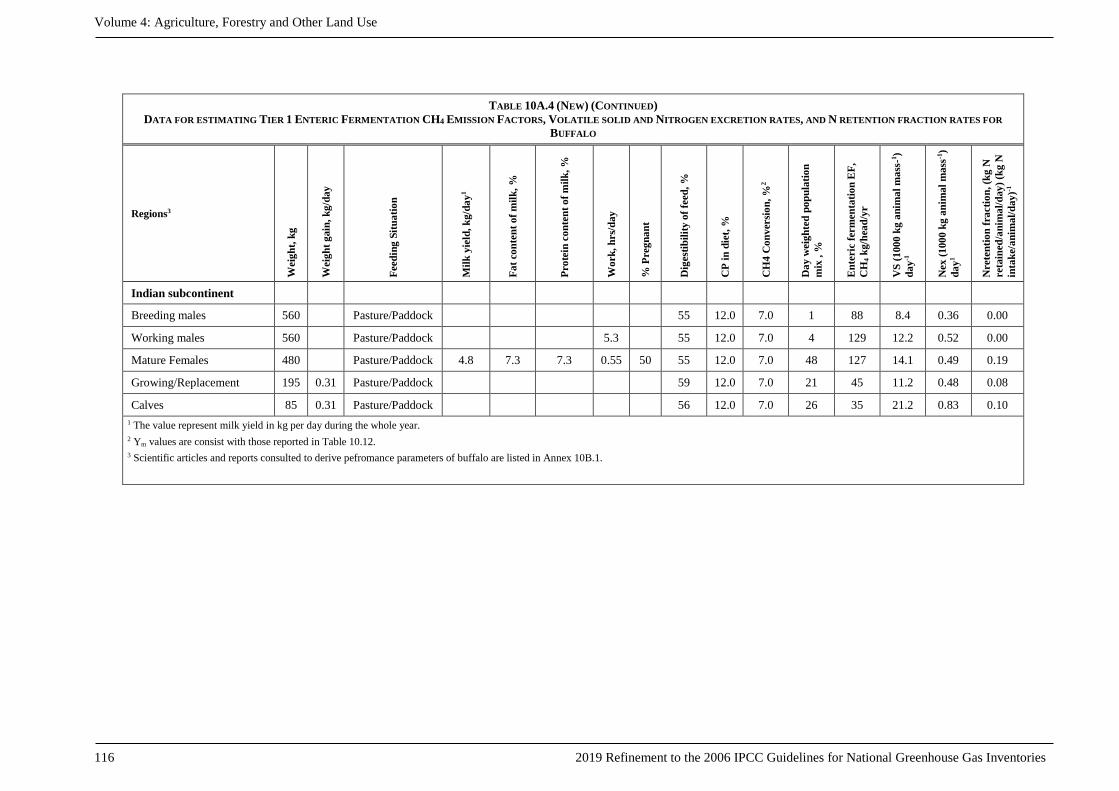
Volume 4: Agriculture, Forestry and Other Land Use
116 2019 Refinement to the 2006 IPCC Guidelines for National Greenhouse Gas Inventories
TABLE 10A.4 (NEW) (CONTINUED)
DATA FOR ESTIMATING TIER 1 ENTERIC FERMENTATION CH4 EMISSION FACTORS, VOLATILE SOLID AND NITROGEN EXCRETION RATES, AND N RETENTION FRACTION RATES FOR
BUFFALO
Regions3
Weig
ht,
kg
Weig
ht
gain
, k
g/d
ay
Feed
ing
Sit
ua
tio
n
Mil
k y
ield
, k
g/d
ay
1
Fa
t co
nte
nt
of
mil
k,
%
Pro
tein
co
nte
nt
of
mil
k, %
Wo
rk
, h
rs/
day
% P
reg
na
nt
Dig
est
ibil
ity
of
feed
, %
CP
in
die
t, %
CH
4 C
on
ver
sio
n, %
2
Da
y w
eig
hte
d p
op
ula
tio
n
mix
, %
En
teri
c f
erm
en
tati
on
EF
,
CH
4 k
g/h
ead
/yr
VS
(1
000
kg a
nim
al
ma
ss-1
)
da
y-1
Nex
(1
000
kg
an
imal
ma
ss-1
)
da
y1
Nrete
nti
on
fra
cti
on
, (k
g N
reta
ined
/an
ima
l/d
ay
) (k
g N
inta
ke/
an
ima
l/d
ay
)-1
Indian subcontinent
Breeding males 560 Pasture/Paddock 55 12.0 7.0 1 88 8.4 0.36 0.00
Working males 560 Pasture/Paddock 5.3 55 12.0 7.0 4 129 12.2 0.52 0.00
Mature Females 480 Pasture/Paddock 4.8 7.3 7.3 0.55 50 55 12.0 7.0 48 127 14.1 0.49 0.19
Growing/Replacement 195 0.31 Pasture/Paddock 59 12.0 7.0 21 45 11.2 0.48 0.08
Calves 85 0.31 Pasture/Paddock 56 12.0 7.0 26 35 21.2 0.83 0.10
1 The value represent milk yield in kg per day during the whole year.
2 Ym values are consist with those reported in Table 10.12. 3 Scientific articles and reports consulted to derive pefromance parameters of buffalo are listed in Annex 10B.1.

Chapter 10: Emissions from Livestoch and Manure Management
2019 Refinement to the 2006 IPCC Guidelines for National Greenhouse Gas Inventories 10.117
Annex 10A.2 Additional data and information for the
calculation of methane and nitrous oxide from
Manure Management
This annex presents the required default data to implement the Tier 1 manure management emissions for methane
and nitrous oxide. Data required in both methods include animal weight data required for the calculation of average
VS and N excretion per animal category as well as AWMS system information for regions around the country and
improved definitional data, relating IPCC AWMS systems and definitions used in the EMEP/EEA air pollutant
emission inventory guidebook. The information is a combination of the consistent data collection in for cattle and
buffalo that is compiled in Annex 10A.1 and data compiled by the FAO for use in their modelling system GLEAM
(FAO 2017; MacLeod et al. 2017). More specific information can be found, sometimes at the country level at
http://www.fao.org/gleam/resources/en/. Furthermore, information is supplied on IPCC climate zones.

Volume 4: Agriculture, Forestry and Other Land Use
10.118 2019 Refinement to the 2006 IPCC Guidelines for National Greenhouse Gas Inventories
TABLE 10A.5 (NEW)
DEFAULT VALUES FOR LIVE WEIGHTS FOR ANIMAL CATEGORIES (KG)
Category of
animal
Region
No
rth
Am
eric
a
Wes
tern
Eu
rop
e
Ea
ster
n E
uro
pe
Oce
an
ia
Latin America Africa Middle East Asia India sub-continent
Mea
n
Hig
h P
S1
Lo
w P
S1
Mea
n
Hig
h P
S
Lo
w P
S
Mea
n
Hig
h P
S
Lo
w P
S
Mea
n
Hig
h P
S
Lo
w P
S
Mea
n
Hig
h P
S
Lo
w P
S
Dairy cattle2 650 600 550 488 508 520 500 260 250 270 349 510 270 386 485 355 285 350 265
Other cattle2 407 405 389 359 303 329 295 236 302 208 275 362 232 299 310 296 226 167 236
Buffalo2 NA 509 467 NA 315 339 381 336 321
Swine3 77 76 77 61 65 81 59 49 72 37 59 70 53 58 69 52 59 68 53
Finishing 61 61 59 41 51 59 47 41 54 33 52 60 48 49 56 44 51 55 48
Breeding 184 190 204 163 143 205 121 100 200 61 118 157 99 122 160 102 121 162 99
Poultry3 1.4 1.4 1.3 1.3 1.1 1.3 0.9 0.9 1 0.8 0.9 1.2 0.7 1.2 1.4 1 1.0 1.2 0.8
Hens >/= 1 yr 1.5 1.9 1.9 2 1.4 1.6 1.3 1.4 1.9 1.1 1.2 1.7 1 1.5 1.9 1.3 1.3 1.5 1.1
Pullets 1.2 1.5 1.3 1.4 0.7 1.3 0.5 0.7 1.4 0.5 0.6 1.2 0.4 0.8 1.5 0.6 0.6 1.3 0.4
Broilers 1.4 1.2 1.1 1.2 0.9 1.2 0.7 0.8 0.8 0.7 0.7 1 0.5 0.8 1 0.7 0.8 1 0.6
Turkeys4 6.8
Ducks4 2.7
Sheep3 40 31
Goats5 41 40 36 33 24
Horses4 377 238
Mules and asses4 130
Camels4 217
Ostrich5 120

Chapter 10: Emissions from Livestoch and Manure Management
2019 Refinement to the 2006 IPCC Guidelines for National Greenhouse Gas Inventories 10.119
TABLE 10A.5 (NEW) (CONTINUED)
DEFAULT VALUES FOR LIVE WEIGHTS FOR ANIMAL CATEGORIES (KG)
Category of
animal
Region
No
rth
Am
eric
a
Wes
tern
Eu
rop
e
Ea
ster
n E
uro
pe
Oce
an
ia
Latin America Africa Middle East Asia India sub-continent
Mea
n
Hig
h P
S1
Lo
w P
S1
Mea
n
Hig
h P
S
Mea
n
Hig
h P
S1
Lo
w P
S1
Mea
n
Hig
h P
S
Mea
n
Hig
h P
S1
Lo
w P
S1
Mea
n
Hig
h P
S
Deer5 120
Reindeer5 120
1 High PS and Low PS refer to high- and low productivity systems required for Tier 1a methodology
2 Values are derived from diets used in the calculation of enteric fermentation Tier 1 and Tier 1a emission factors (Table 10A.1 – Table 10A.4) 3 Values are taken from FAO GLEAM databases (FAO 2017). High and low estimates are simplified extracts from the model database and may be prone to refinement in the final draft. Means of high and low
productivity systems are simple means and will be refined in the final order draft.
4 Values are taken from Table 10A-9 of of the IPCC 2006 IPCC Guidelines 5 For more information see Table 10.10 and Table 10.19 of the 2019 Refinement

Volume 4: Agriculture, Forestry and Other Land Use
10.120 2019 Refinement to the 2006 IPCC Guidelines for National Greenhouse Gas Inventories
TABLE 10A.6 (NEW)
ANIMAL WASTE MANAGEMENT SYSTEM (AWMS) REGIONAL AVERAGES FOR CATTLE AND BUFFALO
Animal Category Climate and System Based
Category
AWMS (%)
Lagoon Liquid
/Slurry
Solid
storage
Drylot Pasture/
Range/
Paddock
Daily
spread
Digester Burned
for fuel
Other
Dairy Cattle North America 26 24 24 0 15 11 0 0 0
Western Europe 0 43 29 0 26 2 0 0 0
Eastern Europe 0 5 74 0 20 1 0 0 0
Oceania 5 0 0 0 94 1 0 0 0
East Asia and South-East Asia
(Asia) 0 1 21 29 38 0 0 11 0
South Asia (Indian subcontinent) 0 0 1 49 30 0 0 20 0
Latin America and the Caribbean 0 0 5 38 57 0 0 0 0
Near East (Middle East) and North
Africa 0 0 14 35 46 0 0 5 0
Sub-Saharan Africa 0 0 20 29 45 0 0 6 0
Non Dairy Cattle North America 0 1 43 14 42 0 0 0 0
Western Europe 0 22 26 0 48 4 0 0 0
Eastern Europe 0 64 5 0 31 0 0 0 0
Oceania 0 0 0 0 100 0 0 0 0
East Asia and South-East Asia
(Asia) 0 0 29 28 36 0 0 7 0
South Asia (Indian subcontinent) 0 0 1 49 30 0 0 20 0
Latin America and the Caribbean 0 0 3 5 92 0 0 0 0
Near East (Middle East) and North
Africa 0 0 5 46 42 0 0 7 0
Sub-Saharan Africa 0 0 15 30 50 0 0 5 0

Chapter 10: Emissions from Livestoch and Manure Management
2019 Refinement to the 2006 IPCC Guidelines for National Greenhouse Gas Inventories 10.121
TABLE 10A.6 (NEW) (CONTINUED)
ANIMAL WASTE MANAGEMENT SYSTEM (AWMS) REGIONAL AVERAGES FOR CATTLE AND BUFFALO
Animal Category Climate and System Based
Category
AWMS (%)
Lagoon Liquid
/Slurry
Solid
storage
Drylot Pasture/
Range/
Paddock
Daily
spread
Digester Burned
for fuel
Other
Buffalo Dairy North America 0 43 40 0 17 0 0 0 0
Western Europe 0 34 63 0 3 0 0 0 0
Eastern Europe 0 18 68 0 13 1 0 0 0
East Asia and South-East Asia
(Asia) 0 0 10 58 29 0 0 3 0
South Asia (Indian subcontinent) 0 0 1 41 38 0 0 20 0
Latin America and the Caribbean 0 0 2 48 50 0 0 0 0
Near East (Middle East) and North
Africa 0 0 18 35 46 0 0 1 0
Buffalo Non dairy Eastern Europe (including Russia) 0 9 64 0 27 0 0 0 0
East Asia and South-East Asia
(Asia) 0 0 6 64 28 0 0 2 0
South Asia (Indian subcontinent) 0 0 1 40 39 0 0 20 0
Latin America and the Caribbean 0 0 2 5 93 0 0 0 0
Near East (Middle East) and North
Africa 0 0 16 12 57 0 0 15 0

Volume 4: Agriculture, Forestry and Other Land Use
10.122 2019 Refinement to the 2006 IPCC Guidelines for National Greenhouse Gas Inventories
TABLE 10A.7 (NEW)
ANIMAL WASTE MANAGEMENT SYSTEM (AWMS) REGIONAL AVERAGES FOR SWINE (%)
Animal
Category
Productivity
class Region Lagoon Liquid/Slurry
Solid
storage Drylot
Pit
<1
Pit >
1
Daily
spread Digester Pasture
Growing
Swine
High
Productivity
North America 28 31 4 3 0 34 0 0 0
Western Europe 6 51 14 0 2 26 1 0 0
Eastern Europe 5 31 55 1 4 4 0 0 0
Russia 0 24 76 0 0 0 0 0 0
Oceania 91 0 1 8 0 0 0 0 0
East Asia and South East Asia 35 21 0 2 35 0 0 7 0
Indian subcontinent 12 23 13 35 2 0 7 8 0
Latin America and the Caribean 11 34 12 41 0 0 2 0 0
Near East (Middle East) and North
Africa 10 29 0 54 0 0 0 7 0
Sub-saharan Africa 0 7 6 86 1 0 0 0 0
Low
Productivity
East Asia and South East Asia 5 27 18 14 14 5 6 5 6
Indian subcontinent 5 30 15 15 15 5 5 5 5
Latin America and the Caribean 5 30 15 15 15 5 5 5 5
Near East (Middle East) and North
Africa 5 30 15 15 15 5 5 5 5
Sub-saharan Africa 5 30 15 15 15 5 5 5 5

Chapter 10: Emissions from Livestoch and Manure Management
2019 Refinement to the 2006 IPCC Guidelines for National Greenhouse Gas Inventories 10.123
TABLE 10A.7 (NEW) (CONTINUED)
ANIMAL WASTE MANAGEMENT SYSTEM (AWMS) REGIONAL AVERAGES FOR SWINE (%)
Animal
Category
Productivity
class Region Lagoon Liquid/Slurry
Solid
storage Drylot
Pit
<1
Pit >
1
Daily
spread Digester Pasture
Breeding
Swine
High
Productivity
North America 28 31 4 3 0 34 0 0 0
Western Europe 6 51 15 0 2 25 1 0 0
Eastern Europe 5 31 55 1 4 4 0 0 0
Russia 0 24 76 0 0 0 0 0 0
Oceania 91 0 1 8 0 0 0 0 0
East Asia and South East Asia 35 21 0 2 35 0 0 7 0
Indian subcontinent 12 23 14 32 3 0 8 8 0
Latin America and the Caribean 11 34 12 41 0 0 2 0 0
Near East (Middle East) and North
Africa 10 29 0 54 0 0 0 7 0
Sub-saharan Africa 0 7 6 86 1 0 0 0 0
Low
Productivity
East Asia and South
East Asia 4 28 22 13 13 4 6 4 6
Indian subcontinent 5 30 15 15 15 5 5 5 5
Latin America and the Caribean 5 30 15 15 15 5 5 5 5
Near East (Middle East) and North
Africa 5 30 15 15 15 5 5 5 5
Sub-saharan Africa 5 30 15 15 15 5 5 5 5

Volume 4: Agriculture, Forestry and Other Land Use
10.124 2019 Refinement to the 2006 IPCC Guidelines for National Greenhouse Gas Inventories
TABLE 10A.8 (NEW)
ANIMAL WASTE MANAGEMENT SYSTEM (AWMS) REGIONAL AVERAGES FOR SHEEP AND GOATS
Animal
Category Region1
AWMS (%)
Lagoon Liquid/Slurry Solid
storage Drylot
Pasture/Range/
Paddock
Daily
spread Digester
Burned for
fuel Other
Sheep - Meat
North America 0 0 54 0 46 0 0 0 0
Western Europe 0 0 13 0 87 0 0 0 0
Eastern Europe 0 0 54 0 46 0 0 0 0
Near East (Middle East) and
North Africa 0 0 0 50 50 0 0 0 0
East Asia and South-East Asia 0 0 17 3 80 0 0 0 0
Oceania 0 0 0 0 100 0 0 0 0
South Asia (Indian subcontinent) 0 0 17 3 80 0 0 0 0
Latin America and the
Caribbean 0 0 17 3 80 0 0 0 0
Sub-Saharan Africa 0 0 17 3 80 0 0 0 0
Sheep - Dairy
Western Europe 0 0 21 0 78 0 0 0 0
Eastern Europe 0 0 42 0 58 0 0 0 0
Near East (Middle East) and
North Africa 0 0 0 50 50 0 0 0 0
East Asia and South-East Asia 0 0 17 3 80 0 0 0 0
South Asia (Indian subcontinent) 0 0 17 3 80 0 0 0 0
Latin America and the
Caribbean 0 0 17 3 80 0 0 0 0
Sub-Saharan Africa 0 0 17 3 80 0 0 0 0

Chapter 10: Emissions from Livestoch and Manure Management
2019 Refinement to the 2006 IPCC Guidelines for National Greenhouse Gas Inventories 10.125
TABLE 10A.8 (NEW) (CONTINUED)
ANIMAL WASTE MANAGEMENT SYSTEM (AWMS) REGIONAL AVERAGES FOR SHEEP AND GOATS
Animal
Category Region1
AWMS (%)
Lagoon Liquid/Slurry Solid
storage Drylot
Pasture/Range/
Paddock
Daily
spread Digester
Burned for
fuel Other
Goat
North America 0 0 50 0 50 0 0 0 0
Russia 0 0 82 0 18 0 0 0 0
Western Europe 0 0 28 0 72 0 0 0 0
Eastern Europe 0 0 9 0 91 0 0 0 0
Near East (Middle East) and
North Africa 0 0 0 50 50 0 0
0 0
East Asia and South-East Asia 0 0 50 0 50 0 0 0 0
Oceania 0 0 0 0 100 0 0 0 0
South Asia (Indian subcontinent) 0 0 50 0 50 0 0 0 0
Latin America and the
Caribbean 0 0 17 3 80 0 0 0 0
Sub-Saharan Africa 0 0 17 3 80 0 0 0 0

Volume 4: Agriculture, Forestry and Other Land Use
10.126 2019 Refinement to the 2006 IPCC Guidelines for National Greenhouse Gas Inventories
TABLE 10A.9 (NEW)
ANIMAL WASTE MANAGEMENT SYSTEM (AWMS) REGIONAL AVERAGES FOR POULTRY AND OTHER1 ANIMALS
Animal
Category Region
AWMS (%)
Lagoon Liquid
/Slurry
Solid
storage Drylot
Pasture/Range
/Paddock
Pit >1
month
Daily
spread Digester
Other (Poultry
manure with
litter)
Chicken-Layer
North America 1 29 70 0 0 0 0 0 0
Russia 0 0 0 0 0 100 0 0 0
Western Europe 0 1 20 21 0 43 1 0 14
Eastern Europe 0 0 0 47 0 34 0 0 19
Near East (Middle
East) and North Africa 11 7 11 0 0 67 0 0 4
East Asia and South-
East Asia 0 4 0 0 1 94 1 0 0
Oceania 0 0 0 0 23 77 0 0 0
South Asia
(Indian subcontinent) 0 0 100 0 0 0 0 0 0
Latin America and the
Caribbean 0 58 42 0 0 0 0 0 0
Sub-Saharan Africa 0 0 0 0 0 90 0 0 10

Chapter 10: Emissions from Livestoch and Manure Management
2019 Refinement to the 2006 IPCC Guidelines for National Greenhouse Gas Inventories 10.127
TABLE 10A.9 (NEW) (CONTINUED)
ANIMAL WASTE MANAGEMENT SYSTEM (AWMS) REGIONAL AVERAGES FOR POULTRY AND OTHER1 ANIMALS
Animal
Category Region
AWMS (%)
Lagoon Liquid
/Slurry
Solid
storage Drylot
Pasture/Range
/Paddock
Pit >1
month
Daily
spread Digester
Other (Poultry
manure with
litter)
Chicken-Broiler
North America 0 0 0 0 0 0 0 0 100
Russia 0 0 0 0 0 0 0 0 100
Western Europe 0 0 0 0 0 0 0 0 100
Eastern Europe 0 0 0 0 0 0 0 0 100
Near East (Middle
East) and North Africa 0 0 0 0 0 0 0 0 100
East Asia and South-
East Asia 0 0 0 0 0 0 0 0 100
Oceania 0 0 0 0 0 0 0 0 100
South Asia 0 0 0 0 0 0 0 0 100
(Indian subcontinent)
Latin America and the
Caribbean 0 0 0 0 0 0 0 0 100
Sub-Saharan Africa 0 0 0 0 0 0 0 0 100

Volume 4: Agriculture, Forestry and Other Land Use
10.128 2019 Refinement to the 2006 IPCC Guidelines for National Greenhouse Gas Inventories
TABLE 10A.9 (NEW) (CONTINUED)
ANIMAL WASTE MANAGEMENT SYSTEM (AWMS) REGIONAL AVERAGES FOR POULTRY AND OTHER1 ANIMALS
Animal
Category Region
AWMS (%)
Lagoon Liquid
/Slurry
Solid
storage Drylot
Pasture/Range
/Paddock
Pit >1
month
Daily
spread Digester
Other (Poultry
manure with
litter)
Low
productivity
North America 0 0 0 0 50 0 50 0 0
Russia 0 0 0 0 50 0 50 0 0
Western Europe 0 0 0 0 50 0 50 0 0
Eastern Europe 0 0 0 0 50 0 50 0 0
Near East (Middle
East) and North Africa 0 0 0 0 50 0 50 0 0
East Asia and South-
East Asia 0 0 0 0 50 0 50 0 0
Oceania 0 0 0 0 50 0 50 0 0
South Asia 0 0 0 0 50 0 50 0 0
(Indian subcontinent)
Latin America and the
Caribbean 0 0 0 0 50 0 50 0 0
Sub-Saharan Africa 0 0 0 0 50 0 50 0 0
1 For Other animal, the IPCC expert group reviewed the national inventory submissions as well as guidance in the 2006 IPCC Guidelines under the UNFCCC and concluded that common distribution of systems
used to manage manure as follows:
Horses, camelelids, mules and asses, and other grazing animals; should use the data supplied for goats as a proxy
Deer and reindeer manure deposited at 100% in PRP
Ostrich (Emu) manure is 80% in PRP and 20 percent managed in solid based systems;
Rabbits and fur-bearing animals is 100% managed in a solid based system.
Hence, countries may apply the same allocation of MMS in the calculation of N2O emissions from manure stored in manure management systems. However, countries are encouraged to develop a country-
specific dataset on MMS used to manage manure generated by these categories of animals.

Chapter 10: Emissions from Livestoch and Manure Management
2019 Refinement to the 2006 IPCC Guidelines for National Greenhouse Gas Inventories 10.129
INFORMATION REQUIRED TO DETERMINE CLIMATE ZONES
ACCORDING TO CHAPTER 3 OF VOLUME 5 CURRENT GUIDELINE
Outlined below are the conditions required to determine the climate zone required for the selection of a party’s
MCF factor, according to the IPCC climate zone determination as defined in Volume 4, Chapter 3, Annex 3A.5,
Figure 3A.5.2. Where possible, if countries span multiple climate zones, efforst should be made to disaggregate
animal populations into climate zones. If this is not possible, partys are advised to select the climate zone covering
the greatest surface area of their country or regions of their country for which they have distinct animal populations.
Briefly, all data is drawn from “The Climate Reseach Unit (CRU) or the CGIAR-Consortium for Spatial
Information (CSI) 1985-2015.” Climate zones are differentiated based on the factors of mean annual temperature,
elevation, mean annual precipitation and the ratio of mean annual precipitation to precipitation for this 30 year
average annual weather data compilation.
Therefore as identified in Chapter 3 of these guidelines climate zones are defined where
Tropical Montane: has >18oC mean annual temperature and at an elevation greater than 1000m;
Tropical Wet: has >18oC mean annual temperature and mean annual precipitation >2000mm;
Tropical Moist: has >18oC mean annual temperature and mean annual precipitation >1000mm;
Tropical Dry: has >18oC mean annual temperature and mean annual precipitation < 1000mm;
Tropical Moist: has >18oC mean annual temperature and mean annual precipitation >1000mm;
Warm temperate moist: has >10 oC mean annual temperature and a ratio of potential evapotranspiration to
prescipitation > 1;
Warm temperate dry: has >10 oC mean annual temperature and a ratio of potential evapotranspiration to
precipitation < 1;
Cool temperate moist: has > 0 oC mean annual temperature and a ratio of potential evapotranspiration to
precipitation >1;
Cool temperate dry: has > 0 oC mean annual temperature and a ratio of potential evapotranspiration to precipitation
<1;
Boreal moist: has < 0 oC mean annual temperature but some monthly temperatures > 10and a ratio of potential
evapotranspiration >1;
Boreal dry: has < 0 oC mean annual temperature but some monthly temperatures > 10 and a ratio of potential
evapotranspiration to precipitation <1;
Polar moist: has < 0 oC mean annual temperature but all monthly temperatures < 10and a ratio of potential
evapotranspiration >1;
Polar dry: has < 0 oC mean annual temperature but all monthly temperatures < 10 and a ratio of potential
evapotranspiration to precipitation <1.

Volume 4 : Agriculture, Forestry and Other Land Use
10.130 2019 Refinement to the 2006 IPCC Guidelines for National Greenhouse Gas Inventories
Figure 10A.1 (New) Mapping of IPCC climate zones. (taken from Volume 4, Chapter 3, Annex 3A.5)

Chapter 10: Emissions from Livestoch and Manure Management
2019 Refinement to the 2006 IPCC Guidelines for National Greenhouse Gas Inventories 10.131
TABLE 10A.10 (NEW)
COMPARISON OF MANURE STORAGE TYPE DEFINITIONS USED BY THE IPCC AND BY THE EMEP/EEA AIR POLLUTANT
EMISSION INVENTORY GUIDEBOOK 2016 (HTTPS://WWW.EEA.EUROPA.EU/PUBLICATIONS/EMEP-EEA-GUIDEBOOK-2016)
System IPCC System EMEP / EEA Definition
Pasture/Range/Paddock (PRP) Grazing
The manure from pasture and range
grazing animals is allowed to lie as
deposited, and is not managed.
Daily spread No definition given
Manure is routinely removed from a
confinement facility and is applied to
cropland or pasture within 24 hours of
excretion.
Solid storage Heaps
The storage of manure, typically for a
period of several months, in unconfined
piles or stacks. Manure is able to be
stacked because of the presence of a
sufficient amount of bedding material or
loss of moisture by evaporation
Dry lot No definition given
A paved or unpaved open confinement
area without any significant vegetative
cover. Dry lots do not require the addition
of bedding to control moisture. Manure
may be removed periodically and spread
on fields.
Liquid/Slurry Tanks
Manure is stored as excreted or with some
minimal addition of water in either tanks
or earthen ponds outside the livestock
building, usually for periods of less than 1
year;
Storage with a low surface area to depth
ratio; normally steel or concrete cylinders
Liquid/Slurry, With natural crust
cover Crust
Natural or artificial layer on the surface of
slurry which reduces the diffusion of
gasses to the atmosphere
Liquid/Slurry, cover Cover
Rigid or flexible structure that covers the
manure and is impermeable to water and
gasses
Uncovered anaerobic lagoon Lagoons
Storage with a large surface area to depth
ratio; normally shallow excavations in the
soil
Pit storage below animal
confinements In-house slurry pit
Mixture of excreta and washing water,
stored within the livestock building,
usually below the confined animals
Anaerobic digester Biogas treatment Anaerobic fermentation of slurry and/or
solid
Burned for fuel No definition given
The dung and urine are excreted on fields.
The sun dried dung cakes are burned for
fuel.
Deep bedding In-house deep litter
Mixture of excreta and bedding,
accumulated on the floor of the livestock
building

Volume 4: Agriculture, Forestry and Other Land Use
10.132 2019 Refinement to the 2006 IPCC Guidelines for National Greenhouse Gas Inventories
TABLE 10A.10 (NEW) (CONTINUED)
COMPARISON OF MANURE STORAGE TYPE DEFINITIONS USED BY THE IPCC AND BY THE EMEP/EEA AIR POLLUTANT
EMISSION INVENTORY GUIDEBOOK 2016 (HTTPS://WWW.EEA.EUROPA.EU/PUBLICATIONS/EMEP-EEA-GUIDEBOOK-2016)
System IPCC System EMEP / EEA Definition
Composting
In-vessel Forced-aeration composting Aerobic decomposition of manure with
forced ventilation
Static pile Composting, passive windrow Aerobic decomposition of manure without
forced ventilation
Intensive
windrow No EMEP equivalent
Composting -
Passive
windrow
No EMEP equivalent
Poultry manure with litter
Laying hens – solid
Broilers – litter
Other poultry - litter
Similar to cattle and swine deep bedding
except usually not combined with a dry lot
or pasture. Typically used for all poultry
breeder flocks, for alternative systems for
layers and for the production of meat type
chickens (broilers) and other fowl. Litter
and manure are left in place with added
bedding during the poultry production
cycle and cleaned between poultry cycles,
typically 5 to 9 weeks in productive
systems and X amount of days in lower
productivity systems.
Poultry manure without litter Laying hens – slurry
May be similar to open pits in enclosed
animal confinement facilities or may be
designed and operated to dry the manure
as it accumulates. The latter is known as a
high-rise manure management system and
is a form of passive windrow composting
when designed and operated properly.
Some intensive poultry farms installed the
manure belt under the cage, where the
manure is dried inside housing.
Aerobic treatment No EMEP equivalent
The biological oxidation of manure
collected as a liquid with either forced or
natural aeration. Natural aeration is limited
to aerobic and facultative ponds and
wetland systems and is due primarily to
photosynthesis. Hence, these systems
typically become anoxic during periods
without sunlight.
No definition given Slurry separation The separation of the solid and liquid
components of slurry
No definition given Acidification The addition of strong acid to reduce
manure pH

Chapter 10: Emissions from Livestoch and Manure Management
2019 Refinement to the 2006 IPCC Guidelines for National Greenhouse Gas Inventories 10.133
Annex 10A.3 Spreadsheet example for the calculation of a
country or regions specific MCF
MCF CALCULATIONS AND EXAMPLE SPREADSHEET
This Annex was developed to explain how MCF factors in the guidelines have been derived and to provide a
detailed step by step protocol for inventory compilers to calculate country or region specific MCFs. Application
of the model at the national scale requires national or regional monthly air temperature profiles as well as the
average number and timing of the emptying of manure storages. Temperature data can be downloaded from various
agencies such as the National Oceanic and Atmospheric Andministration (NOAA) or the European Environmental
Agency. Manure removal statistics may be taken from farm practice surveys or from expert consultation.
Compilers should develop an estimate of the average number of manure removals per year and the months of the
highest frequency of removals. If regional practices vary within a country, compilers should develop MCFs that
are representative of regional practice by entering consistent manure removal statistics with regional temperature
profiles. If regional MCFs are calculated, the national MCF should be weighted based on the number of animals
feeding into the regional manure management systems represented by the manure removal profile and the regional
temperature profile.
Further, to support the IPCC Guidance Document, a spreadsheet was created to enable users to calculate a site-
specific Methane Conversion Factor (MCF). The spreadsheet uses the same calculations that were used to
calculated the MCF Table in the guidance document, but has been designed with a user in mind available in the
supplemental data supplied with this Chapter, maintained on the IPCC document website, there identified as
Supplemental Information Chapter 10, Volume IV, 2019 Refinement.
The calculation procedure outlined in the spreadsheet contains three main sections:
Inputs to the model;
Model calculations;
Results from the model.
As an explanation of procedures, within each section, cells are colour coded. Compilers are required to develop
input data for anything that is indicated by yellow highlighted cells, and have the option of editing the orange
highlighted cells if needed, but only if country-specific information is available for those parameters. Other cells
are not meant to be edited by the user.
Figure 10A.2 (New) Colour code for cells in the example spreadsheet
MODEL INPUT
Temperature
The Input required to run the model at a national scale and recreate the spreadsheet is shown below (Figures 2 and
3). In this section, the compiler should input 12 months of temperature data (degrees C) in cells D9:D20, based on
average monthly temperatures for the region for which they wish to develop the MCF.
If the compiler has estimates of national or regional manure temperature, they should select “Manure” in cell D6.
As a result, the spreadsheet will copy the user-input temperature into cells E9:E20, for further use in the analysis.
If the compiler is using national or regional air temperature (not manure temperature), they should select “Air” in
cell D6. As a result, the spreadsheet will generate an estimate for manure temperature in cells E9:E20. The
estimates are based on the following logic:
Manure temperature lags 1-month behind air temperature.
o e.g., Tmanure in June = Tair in May.
The minimum manure temperature will be used (1 degree C by default; user adjustable)
o e.g., for Tair = -9 C, Tman = 1 C

Volume 4: Agriculture, Forestry and Other Land Use
10.134 2019 Refinement to the 2006 IPCC Guidelines for National Greenhouse Gas Inventories
If and only if the storage is emptied once per year, manure temperature will be reduced by a dampening factor (3
degrees C by default; user adjustable).
i.e. Tman = Tair – damping factor; e.g., 12 = 15 – 3
The logic equation is implemented in Excel as follows, for example, in cell E9:
=IF($D$6="Manure",D9,IF($F$21>1,MAX(D20,f_Tmin),MAX(D20-f_T2damping,f_Tmin)))
Broken into steps:
If $D$6="Manure" then the result in E9 will equal D9
If $D$6 is not "Manure" (i.e. it is “Air”) then the second IF statement is operated
IF $F$21>1 (i.e. multiple removals per year), then no damping is applied
Manure temperature is selected as air temperature from the previous month, and it is always
greater or equal to the minimum temperature,
i.e. E9 will equal MAX(D20,f_Tmin). In this case, D20 (-6.7) is less than the minimum, so the
result in E9 is the minimum (1.0).
IF $F$21=1 then damping is applied
Damping is applied by subtracting the damping factor: D20-f_T2damping
The temperature is always greater or equal to the minimum temperature, using the MAX() function.
The compiler should then identify the months when manure is removed from the storage in column F (F9:F20).
This can be indicated by a “Y” indicating months when manure was removed, and an “N” for months when manure
is not removed. The number of months when manure was removed is counted and displayed in cell F21.

Chapter 10: Emissions from Livestoch and Manure Management
2019 Refinement to the 2006 IPCC Guidelines for National Greenhouse Gas Inventories 10.135
Figure 10A.3 (New) Temperature and manure removal inputs to the model
Note. Top panel: alphanumeric values in each cell. Middle panel: dropdown menu to select “Air” or “Manure”.
Bottom panel: all formulae are visible.
Constants and Other Input Para meters
The inventory compiler is required to provide several other inputs in the section shown below (Fig. 3). The name
of each parameter is provided in column H, the numeric value of the parameter is in column I, the units are in
column J, the source each value are given in column K, additional notes are in columns L and M, default values
are in column N. To make equations more easily understood, the Microsoft Excel feature of “Named Cells” has
been used to name the cells in column I, and the name of each cell is shown in column O for convenience. For
example, cell I7 is given the name “VS_PROD_YR”. See Figure 3 for a full list of named cells.
Additional information about the input parameters:
VS Excretion – based on IPCC guidance.
VS percent liquid storage – this indicates what percentage of excreted VS is handled as a liquid. For example.
100 percent indicates that all excreted VS enters the liquid storage;
A lower number (say, 75 percent) could indicate that a portion of the solids are separated by a screwpress and
handled as a solid (25 percent) while the remaining 75 percent is handled as liquid;
The compiler must provide a B0 value for the manure. Refer to IPCC guidance;
The compiler may, optionally, adjust the minimum temperature (and temperature damping factors;

Volume 4: Agriculture, Forestry and Other Land Use
10.136 2019 Refinement to the 2006 IPCC Guidelines for National Greenhouse Gas Inventories
The compiler also has the option to adjust the emptying efficiency, which indicates the percentage of manure
removed from storage at each removal. By default this is set to 95 percent, indicating that 5 percent of the VS
remain in storage after emptying. Set this value to 100 percent for complete removal.
Figure 10A.4 (New) Constants and other input parameters for the model
Note. Constants and other input parameters for the model are shown in the top panel. Named Cells in column I are
shown in column O, and in the Name Manager dialog box (bottom panel). No formulae exist in this part of the
spreadsheet.
MODEL CALCULATIONS
The model calculations are run for three years, in order to ensure VS available has stabilized on an annual basis.
For example, in Figure 4, we see that VS Available (column J) increases substantially from the first year to the
second year (J64 vs J65), and then stabilizes in the third year (J66). This is because the first year begins from a
perfectly empty storage, whereas the second year is emptied according to the Emptying Efficiency parameter (95
percent removed / 5 percent remaining; Figure 3).
The model approach is as follows:
Column B: Month of year, over 3 years. These month numbers are used to extract input data shown in Figure 2.
Column C: Average manure temperature in each month. This is extracted from cells E9:E20 (Fig. 2) using a
VLOOKUP function (Figure 5).
Column D: temperature is converted from Celsius to Kelvin, using Excel’s CONVERT function (Fig. 5).
Column E: the temperature-dependent f parameter is calculated using the van’t Hoff-Arrhenius equation (Mangino
et al. 2001; IPCC 2006), with updated input parameters shown in Figure 3.
Column F: monthly VS excreted is calculated by dividing the annual VS input parameter by 12.
Column G: monthly VS loaded is calculated by multiplying VS excreted by the percentage stored as liquid. In this
example, the two are equal because VS_PCT_LIQUID is 100 percent (Fig. 3).
Column H: monthly manure emptying is extracted from cells F9:F20 (Fig. 2) using a VLOOKUP function (Fig.
5).

Chapter 10: Emissions from Livestoch and Manure Management
2019 Refinement to the 2006 IPCC Guidelines for National Greenhouse Gas Inventories 10.137
Column I: the quantity of VS emptied is calculated. The logic is as follows: if emptying occurred, then calculate
the mass of VS available to be removed using the mass of VS available in the previous month minus the mass of
VS consumed in the previous month. Then, multiply the result by the EMPTY_EFFICIENCY parameter (Fig. 3,
5).
Column J: the mass of VS available for producing methane is calculated. In the first month of the first year this is
equal to the mass of VS loaded. In all other months, this is calculated as the VS loaded in the current month + VS
available in the previous month – VS consumed in the previous month – VS emptied in the current month.
Column K: the mass of VS consumed is calculated by multiplying VS available by f.
Column L: the volume of CH4 produced is calculated by multiplying VS consumed by B0.
Using these values and equations, the compiler should be able to reproduce graphics such as the profile of manure
temperature, volatile solids and methane production shown in Figure 6.
Figure 10A.5 (New) Monthly model inputs and outputs over a three year period

Volume 4: Agriculture, Forestry and Other Land Use
10.138 2019 Refinement to the 2006 IPCC Guidelines for National Greenhouse Gas Inventories
Figure 10A.6 (New) Formulae used in the model
Note. To conserve space, only 12 months are shown. Top panel: Temperature in oC (Column C and D), coefficient
(Column E), VS excreted, (Column F) and VS loaded (Column G). Middle panel: month of emptying (Columns
H), VS emptied (Column I), VS available (Column J), VS consumed (Column K) and CH4 Produced (Column L).
Bottom panel: sums in rows 64:66 for selected columns.

Chapter 10: Emissions from Livestoch and Manure Management
2019 Refinement to the 2006 IPCC Guidelines for National Greenhouse Gas Inventories 10.139
Figure 10A.7 (New) Example of monthly patterns in Year 3: manure temperature, VS
available (kg), VS emptied (kg), and methane production.
MODEL RESULTS
The MCF is calculated in the Results section. This is done using the third year outputs. In this particular example,
the input air temperature is from the Cool Temperate Moist region and the retention time is 6-months. The resulting
MCF (21 percent) is identical with the guidance document (21 percent).
Figure 10A.8 (New) Summary of Year 3 VS and methane production, and calculation of
MCF.
Note. Top panel shows results, bottom panel shows equations.
NOTE ABOUT TERMINOLOGY:
The terms “VS Available” and “VS Consumed” are used here to be consistent with IPCC 2006 and Mangino et al.
2001 approach. However, these terms require some clarification to avoid misinterpretation. (1) The term “VS

Volume 4: Agriculture, Forestry and Other Land Use
10.140 2019 Refinement to the 2006 IPCC Guidelines for National Greenhouse Gas Inventories
Consumed” does not represent the real VS degraded but a conceptual quantity of VS removed from the liquid/slurry storage
against the total biomethane potential at 35°C (i.e. the conceptual proportion of the B0 consumed at that point). Therefore,
just as B0 reports the quantity of CH4 produced per kg of VS (i.e. all fractions, degradable and non-degradable),
the concept of “VS Consumed” removes all fractions of VS from storage. This approach is convenient because it
uses the B0 as the integrator of all fractions of VS degradability, and reports the total methane produced from all
fractions as if they were incubated for infinite time, while the f parameter introduces a temperature dependence.
Though this is convenient for modeling, and is consistent with the B0, this does not represent the physical reality of
the liquid/slurry storage. (2) Since “VS Consumed” does not equate with the amount of VS degraded in the storage,
the “VS available” does equate with the amount of VS that would actually be measured in a storage. Therefore,
researchers should not attempt to compare measured VS with “VS available”. (3) The strength of this approach is
its simplicity and the fact that the maximum amount of methane that can be produced is equal to the total VS
produced multiplied by the B0. In other words, the model cannot produce more methane than the B0. (4) The MCF
is the ratio of predicted “VS Consumed” to the total VS that entered the storage over one year. The method does
not address VS destruction. If the “VS Consumed” were multiplied by B’ (m3 CH4/kg VS destroyed), the result
be would be erroneous because “VS Consumed” is not VS Destroyed. This is not to say that B’ cannot be used to
model methane production, but simply that it is not compatible with the “VS Consumed” concept. (5) Although
B0 does not need to enter the MCF calculation, the role of B0 is to be multiplied by the MCF, as stated in equation
10.23 of IPCC (2006).

Chapter 10: Emissions from Livestoch and Manure Management
2019 Refinement to the 2006 IPCC Guidelines for National Greenhouse Gas Inventories 10.141
Annex 10A.4 Calculations of Methane Conversion Factors
(MCFs) factors for biogas systems
MCFs for the biogas digester
Biogas digesters are an important manure management systems. There are different types of biogas digesters,
including centralised biogas digester plants, animal farm based biogas digesters,and digesters that co-digest animal
manures and organic residues. Some biogas digesters such as farm based biogas digesters may include prestorage,
like pit storage below animal confinement, or outdoor storage;; Co-digestion may include energy crops, and/or
different types of organic waste in varying combinations.
Default methane conversion factors (MCFs) of biogas digesters are provided in Table 10.17 and Table 10A.11.
MCFs depend on the amount of B0 that is realised under on farm conditions and on the amount of produced biogas
that leakes from the biogas plant either during storage or energy during production. Calculations to identify default
factors were carried out by varying the level of leakage from the biogas installations. Calculations are based on a
modification of the default values in Table 10.17 and Table 10A.11using the equation defined in Haenel et al.
(2018).
TABLE 10A.11 (NEW)
METHANE CONVERSION FACTOR (MCFDG) INCLUDING BIOGAS DIGESTER AND DIGESTATE STORAGE1
Biogas digester quality Storage gastight level Climate Zone
cold temperate warm
high quality biogas
digester,Ldig=0.01
High quality gastight storage Lsto,gt
=0.01 1.00% 1.00% 1.00%
Low quality gastight storage Lsto,gt
=0.1 1.41% 1.41% 1.41%
open storage Lsto,gt=1 3.55% 4.38% 4.59%
Average 1.99% 2.27% 2.33%
low quality biogas
digester,
Ldig=0.1
High quality gastight storage
Lsto,gt=0.01 9.59% 9.59% 9.59%
Low quality gastight storage Lsto,gt
=0.1 10.00% 10.00% 10.00%
open storage Lsto,gt =1 12.14% 12.97% 13.17%
Average 10.58% 10.85% 10.92%
1 the value of MCF for digestate storage (MCFngts) is based on the MCF value of anaerobic lagoon.
Methane emissions from biogas digesters include the unused biogas (can be defined as leakage) and emissions
from storage of the digestate. The MCF calculation from biogas digesters should be based on the following
equation (Haenel et al., 2018):
EQUATION 10A.1 (NEW)
CALCULATION OF MCF FOR THE COMBINATION “DIGESTER + DIGESTATE STORAGE”
4 4 4 4, , , 0 ,
0
•CH prod CH used CH flared residues CH prod
dg
v v v MCF B vMCF
B
Where:
dgMCF = effective methane conversion factor for the combination “digester + digestate storage”,
percent
4 ,CH prodv = specific volume of methane produced in the digester (related to VS input), m3 CH4 kg-1 VS
4 ,CH usedv = specific volume of methane used for energy production (related to VS input), m3 CH4 kg-1
VS

Volume 4: Agriculture, Forestry and Other Land Use
10.142 2019 Refinement to the 2006 IPCC Guidelines for National Greenhouse Gas Inventories
4 , CH flaredv = specific volume of methane flared (related to VS input), m3 CH4 kg-1VS
residuesMCF = methane conversion factor for the storage of digested manure, percent
0B = maximum methane producing capacity per kg of VS input T, m3 CH4 kg-1 of VS excreted
In practice, the residence time necessary to fully exploit the maximum methane producing capacity 0B is not fully
reached in the gas collection system. In the following, the difference, i.e. the potentially still purgeable amount of
gas ( 0B –4 ,CH prodv ), is denoted as “potential of residual gas” that is assumed to be known, and the ratio of which to 0B is
described by the entity μrgs:
EQUATION 10A.2 (NEW)
CALCULATION OF RELATIVE AMOUNT OF POTENTIAL OFF GAS RELATED TO B0
40 ,
0
CH prod
rg
B v
B
Where:
rg = relative amount of residual gas related to B0 (with 0 ≤ μrg ≤ 1 m3 m-3)
0B = maximum methane producing capacity per kg of VS, m3 CH4 kg-1 VS
4 ,CH prodv = specific volume of methane produced in the digester (related to VS input), m3 CH4 kg-1 VS
In practice, the amount of residual gas, rg is not given as a share of the maximum methane producing capacity
B0, but as a share of the amount of gas usable for energy production. Hence, a new entity νrg can be defined which
is closely related to rg .
The rg can be calculated as follows:
EQUATION 10A.3 (NEW)
CALCULATION OF RELATIVE AMOUNT OF RESIDUAL GAS RELATED TO B0
1
rg
rg
rg
v
v
Where:
rg = relative amount of residual gas related to B0 (with 0 ≤ rg ≤ 1 m3 m-3)
rgv = relative amount of residual gas related to νCH4,prod (with 0 ≤ rgv ≤ 1 m3 m-3)
EQUATION 10A.4 (NEW)
CALCULATION OF RELATIVE AMOUNT OF RESIDUAL GAS RELATED TO CH4 PRODUCTION
4
4
0 ,
rg
,
CH prod
CH prod
B vv
v
Where:
rgv = relative amount of residual gas related to νCH4,prod (with 0 ≤ νrg ≤ 1 m3 m-3)
0B = maximum methane producing capacity per kg of VS, m3 CH4 kg-1VS
4 ,CH prodv = specific volume of methane produced in the digester, (related to VS input) m3 CH4 kg-1VS

Chapter 10: Emissions from Livestoch and Manure Management
2019 Refinement to the 2006 IPCC Guidelines for National Greenhouse Gas Inventories 10.143
The term 4 ,CH prodv –
4 ,CH usedv –4 , CH flaredv in equation 10A.1 is part of the digester’s methane balance (related to
VS input) which can be completed by the methane loss 4 ,CH leakv due to leakage.
EQUATION 10A.5 (NEW)
DIGESTER’S METHANE BALANCE
4 4 4 4, , , , 0CH prod CH used CH flared CH leakv v v v
Where:
4 ,CH prodv = specific volume of methane produced in the digester (related to VS input), m3 CH4 kg-1 VS
4 ,CH usedv = specific volume of methane used for energy production (related to VS input), m3 CH4 kg-1
VS
4 , CH flaredv = specific volume of methane flared (related to VS input), m3 CH4 kg-1VS
4 ,CH leakv = specific volume of methane due to leakage and maintence works (related to VS input), m3
CH4 kg-1 VS
The loss of methane 4 ,CH leakv due to leakage is calculated as part of the total amount of CH4 produced in the
digester. The ratio of these two quantities is defined as the leakage rate digL of the digester. digL is assumed to be
known.
EQUATION 10A.6 (NEW)
CALCULATION OF METHANE LEAKAGE RATE OF DIGESTER
4, 4,•CH leak dig CH prodv L v
Where:
4 ,CH leakv = specific volume of methane due to leakage and maintenance works (related to VS input),
m3 CH4 kg-1 VS
digL = leakage rate of the digester, related to νCH4,prod (with 0 ≤𝐿dig≤ 1 m3 m-3).
4 ,CH prodv = specific volume of methane produced in the digester (related to VS input), m3 CH4 kg-1 VS
In order to give the effective methane conversion factor of the combination, “digester + digestate storage” as a
function of the three parameters, “relative amount of residual gas”, “leakage rate” and “MCF of the digestate
storage”, the methane conversion factor of the combination, “digester + digestate storage” can be calculated as
follows (Equation 10A.7):
EQUATION 10A.7 (NEW)
CALCULATION OF METHANE CONVERSION FACTOR
•1 •dg rg dig rg residuesMCF L MCF
Where:
dgMCF = effective methane conversion factor for the combination “digester + digestate storage”,
percent
rg = relative amount of residual gas related to B0 (with 0 ≤ rg ≤ 1 m3 m-3).
digL = leakage rate of the digester, related to νCH4,prod (with 0 ≤ digL ≤ 1 m3 m-3).

Volume 4: Agriculture, Forestry and Other Land Use
10.144 2019 Refinement to the 2006 IPCC Guidelines for National Greenhouse Gas Inventories
residuesMCF = methane conversion factor for the storage of digested manure, percent.
For the factors of digL and µrg it is recomended to use country-specific data; if country specific data areunavailable.
the following procedure is recommenced: For high quality biogas digesters, the default digL is recommended to
be 0.01 (Rösemann et al. 2017); for low quality biogas digesters, digL is recommended to be 0.01 (Rösemann et
al. 2017); for low quality biogas digesters, digL = 0.1 is recommended (Table 10A-4 to Table 10A-9 2006 IPCC
guidelines). The value of 0.046 is used for µrg based on Haenel et al., (2018) The values presented in Table
10A.11 are derived using equation 10A.7 and the values cited here. Pre-storage loss estimates are not included as
no default values can be identified from the literature. Also, it is assumed that these losses will be low as they
represent economic losses due to lower biogas production. However equations are included below if compilers
wish to adapt their emission estimates to country-specific circustances.
It is assumed that even a gastight storage of digestate has a certain leakage. This leakage rate is described by the
storage-specific leakage rate ,sto gtL . Taking into account the leakage rate and the relative share of gastight storage
of digestate gtsx , the residuesMCF can be calculated following Equation 10A.8:
EQUATION 10A.8 (NEW)
CALCULATION OF METHANE CONVERSION FACTOR OF RESIDUES
,• 1 •sto gt ngtsresidues gts gtsMCF x L x MCF
Where:
residuesMCF = methane conversion factor for the storage of digestate, percent
gtsx = share of gastight storage of the digestate, percent
,sto gtL = leakage rate of the gastight storage (with 0 ≤ ,sto gtL ≤ 1 m3 m-3). For high quality gastight
storage of the digestate ,sto gtL is assumed to be 0.01 m3 m-3. For low quality gastight storage
of the digestate, ,sto gtL is assumed to be 0.1 m3 m-3. For open storage of the digestate,
,sto gtL is assumed to be 1.0 m3 m-3
ngtsMCF = methane conversion factor for the non-gastight storage of digestate, percent. It is assumed
that MCFngts is same to the storage of raw manure.
Biogas plants that are fed with animal manures have, as a rule, a pre-storage for the feedstock before it enters the
digester. The CH4 losses from the pre-storage reduce the CH4 production potential in the digester and the storage
of the digestate. This could be taken into account by modifying equations 10A.7. As a consequence Equation
(10A.7) is transformed to the MCFdg+ps equation as equation 10A.9.
EQUATION 10A.9 (NEW)
CALCULATION OF METHANE CONVERSION FACTOR FOR THE COMBINATION “PRESTORAGE +
DIGESTER + DIGESTATE STORAGE”
rg dig rg
dg+ps 1
( ) ) ]1 [(1
p
ps ps
s ps resid
dg
ues
MCF MCF MCF MCF
MCF MCF L MCF
Where:
dg+psMCF = effective methane conversion factor for the combination “prestorage + digester +digestate
storage”, percent
psMCF = methane conversion factor for prestorage, percent; Table 10.17 provided the default values
for different prestorage.

Chapter 10: Emissions from Livestoch and Manure Management
2019 Refinement to the 2006 IPCC Guidelines for National Greenhouse Gas Inventories 10.145
dgMCF = methane conversion factor for combination “digester+digestate storage”,percent, see
above.
rg = relative amount of residual gas related to B0 (with 0 ≤ rg ≤ 1 m3 m-3).
digL = leakage rate of the digester, related to νCH4,prod (with 0 ≤ digL ≤ 1 m3 m-3)
residuesMCF = methane conversion factor for the storage of digestate (in m3 m-3).

Volume 4: Agriculture, Forestry and Other Land Use
10.146 2019 Refinement to the 2006 IPCC Guidelines for National Greenhouse Gas Inventories
Annex 10A.5 Equations relating all direct and indirect N2O
emissions from manure along all stages in
agricultural production for livestock
As explained in section 10.5.6, nitrogen excreted by animals contribute to several direct and indirect N2O emission
as it cascades through livestock and crop cultivation systems. It is therefore crucial to accurately estimate nitrogen
excretion coefficients. The total direct and indirect N2O emissions associated with the excretion of nitrogen of an
animal type is an important quantity to assess the benefit from improving the estimation of the N-excretion
coefficient for that animal type. However, the total direct and indirect N2O emissions from animal excretion cannot
be easily estimated using the equations given in Chapter 10 and 11 of the Guidelines and their Refinements. This
annex provides a set of equations, based on the equations given in Chapter 10 and 11, that allow the quantification
of total direct and indirect N2O emissions from nitrogen excretion of each animal type T. They are reported in
Equations 10A.10 through 10A27.
The definition of the symbols used in the set of equations is given below Equation 10A.27, grouped by symbols.
Note that for internal consistency, the symbol N is used for all nitrogen flows in kg N animal-1 yr-1; the symbol F
is used for all animal-independent nitrogen flows or nitrogen flows for the total animal population in kg N yr-1; the
symbol Frac is used for all fractions in kg N (kg N)-1 or percent, the symbol EF is used for all N2O emission factors
in kg N2O-N (kg N)-1, and the symbol N2O is used for all N2O emissions in kg N2O-N yr-1 . Not in all cases
therefore, the symbols are identical to those used in the Equations given in Chapters 10 and 11.
EQUATION 10A.10 (NEW)
TOTAL N2O EMISSIONS FOR ANIMAL TYPE T
2 ( ) 2 ( ) 2 ( ) 2 ( )T mm T AM T PRP TN O N O N O N O
EQUATIONS 10A.11 AND 10A.12 (NEW)
TOTAL N2O EMISSIONS FROM MANURE MANAGEMENT FOR ANIMAL TYPE T
2 ( , ) 2 ( , ) 2 ( , ) 2 ( , )mm T D mm T G mm T L mm TN O N O N O N O
2 ( ) ( , ) 3( ) 4 5( , ) ( , )
44
28mm T mm T S S GasMS LeachMST S T S
S
N O F EF Frac EF Frac EF
EQUATIONS 10A.13 THROUGH 10A.14 (NEW)
TOTAL, DIRECT AND INDIRECT N2O EMISSIONS FROM THE APPLICATION OF MANURE TO
MANAGED SOILS FOR ANIMAL TYPE T
2 ( ) 2 , ( ) 2 , ( )AM T D AM T I AM TN O N O N O
2 , ( ) 1 1
441
( ) , , 28D AM TN O F Frac EF Frac EF
AM T AM Rice AM Rice FR
2 , ( ) ( ) 4 ( ) 5
44
28I AM T AM T GASM LEACH HN O F Frac EF Frac EF

Chapter 10: Emissions from Livestoch and Manure Management
2019 Refinement to the 2006 IPCC Guidelines for National Greenhouse Gas Inventories 10.147
EQUATION 10A.15 (NEW)
TOTAL AMOUNT OF ANIMAL MANURE N APPLIED TO SOILS OTHER THAN BY GRAZING ANIMALS
FOR ANIMAL TYPE T
( ) , ,,
1- ••AM T LossMS codigestatemm T S bedding T S APPL TT SS
F F Frac F F Fracå
EQUATION 10A.16 (NEW)
FRACTION OF TOTAL ANIMAL MANURE N LOST IN MANURE MANAGEMENT SYSTEMS FOR
ANIMAL TYPE T
2( , ) ( , ) ( , ) (, ) 3 , LossMS T S GASMS T S LEACHMS T S N MS S S
Frac Frac Frac Frac EF
EQUATION 10A.17 (NEW)
FRACTION OF ANIMAL MANURE N AVAILABLE FOR APPLICATION TO MANAGED SOILS, APPLIED
TO MANAGED SOILS FOR ANIMAL TYPE T
( ) ( ) ( ) ( )1APPL T FEED T FUEL T CNST TFrac Frac Frac Frac
EQUATION 10A.18 THROUGH 10A.19 (NEW)
TOTAL, DIRECT AND INDIRECT N2O EMISSIONS FROM N IN URINE AND DUNG DEPOSITED BY
GRAZING ANIMALS ON PASTURE, RANGE AND PADDOCK (TIER 1) FOR ANIMAL TYPE T
2 ( ) 2 , ( ) 2 , ( )PRP T D PRP T I PRP TN O N O N O
2 , ( ) , ( ) 3 , , ( ) 3 ,
44
28D PRP T PRP CPP T PRP CPP PRP SO T PRP SON O F EF F EF
2 , ( ) ( ) 4 ( ) 5
44
28I RPR T RPR T GASM LEACH HN O F Frac EF Frac EF
EQUATION 10A.20 (NEW)
RELATIONSHIP BETWEEN AVERAGE ANNUAL NITROGEN FLOWS ASSOCIATED WITH AN
INDIVIDUAL ANIMAL [KG N ANIMAL-1 YR-1] AND THE ANNUAL NITROGEN FLOW FOR THE ANIMAL
POPULATION OF LIVESTOCK CATEGORY/SPECIES T IN A COUNTRY [KG N YR-1]
( )TF POP N

Volume 4: Agriculture, Forestry and Other Land Use
10.148 2019 Refinement to the 2006 IPCC Guidelines for National Greenhouse Gas Inventories
EQUATION 10A.21 (NEW)
TOTAL MANURE-N EXCRETED
( ) ( ) ( )T MMS T PRP TN N N
EQUATION 10A.22 AND 10A.23 (NEW)
NITROGEN EXCRETION CALCULATED EITHER USING A DEFAULT FRACTION OF RETENTION (TIER
1) OR DIRECTLY FROM RETENTION DATA
( ) ( ) ( )• 1-T intake T RET TNex N Frac
( ) int ( ) ( )T ake T RET TNex N N
EQUATION 10A.24 (NEW)
TOTAL MANURE-N IN MANURE MANAGEMENT AND STORAGE SYSTEMS
( ) ( ) ( ) ( , )MMS T T T S T S
S
N POP Nex Frac
EQUATION 10A.25 (NEW)
MANURE-N MANAGED IN SYSTEM S
( , ) ( ) ( ) ( , )• •mm T S T T S T SN POP Nex Frac
EQUATION 10A.26 (NEW)
MANURE-N DEPOSITED BY GRAZING ANIMALS, WITH X=CPP,SO
( ) ( ) ( ) ( , )PRP X X X S X GN POP Nex Frac
EQUATION 10A.27 (NEW)
N IN BEDDING MATERIAL ADDED TO MANAGED MANURE
( , ) ( ) ,( , )bedding T S T beddingMS T SN POP N
Where
( )TPOP = number of head of livestock species/category T in the country
Annual total nitrogen flows, F, and annual average nitrogen flows per head, N:
( )TF and ( )TN = animal manure nitrogen excreted for livestock species/category T in the
country, kg N yr-1 and kg N animal-1 yr-1
codigestateF = amount of nitrogen from co-digestates added to biogas plants, kg N yr-1

Chapter 10: Emissions from Livestoch and Manure Management
2019 Refinement to the 2006 IPCC Guidelines for National Greenhouse Gas Inventories 10.149
( )MMS TF and ( )MMS TN = animal manure nitrogen excreted for livestock species/category T in manure
management and storage systems in the country, kg N yr-1 and kg N animal-1
yr-1
( )PRP TF and ( )PRP TN = animal manure nitrogen excreted for livestock species/category T on pasture,
range and paddock in the country, kg N yr-1 and kg N animal-1 yr-1
, ( )PRP CPP TF and , ( )PRP CPP TN = animal manure nitrogen excreted for cattle, pig and poultry species/category
T on pasture, range and paddock in the country, kg N yr-1 and kg N animal-1 yr-
1
, ( )PRP SO TF and , ( )PRP SO TN = total animal manure nitrogen excreted for sheep and other livestock
species/category T on pasture, range and paddock in the country, kg N yr-1 and
kg N animal-1 yr-1
( , )mm T SF and ( , )mm T SN = animal manure nitrogen excreted for livestock species/category T in manure
management and storage system S in the country, kg N yr-1 and kg N animal-1
yr-1
( , )bedding T SF and ( , )bedding T SN = nitrogen in bedding material added for livestock species/category T in
manure management and storage system S in the country, kg N yr-1 and kg N
in bedding animal-1 yr-1
( , )AM T SF and ( , )AM T SN = annual amount of animal manure N applied to soils for each livestock
species/category T, kg N yr-1 and kg N animal-1 yr-1
( )intake TF and ( )intake TN = annual intake of N in feed for each livestock species/category T, kg N yr-1
and kg N animal-1 yr-1
( )retention TF and ( )retention TN = annual retention of N each livestock species/category T, kg N yr-1 and kg N
animal-1 yr-1
( )ex TF and ( )ex TN = annual average N excretion of species/category T in the country, kg N animal-
1 yr-1
Annual N2O emissions for the total population of each livestock species/category T
2 ( )TN O = total annual N2O emissions
2 ( )mm TN O = total annual N2O emissions from Manure Management for each livestock
species/category T in the country, kg N2O yr-1
2 , ( )D mm TN O = direct annual N2O emissions from Manure Management for each livestock
species/category T in the country, kg N2O yr-1
2 , ( )G mm TN O = indirect annual N2O emissions from volatilization of NH3+NOx from Manure
Management for each livestock species/category T in the country, kg N2O yr-1
2 , ( )L mm TN O = indirect annual N2O emissions from leaching and run-off from Manure
Management for each livestock species/category T in the country, kg N2O yr-1
2 ( )AM TN O = total annual N2O emissions from manure nitrogen applied to cultivated soils
for each livestock species/category T, kg N2O yr-1
2 ( )PRP TN O = total annual N2O emissions from manure nitrogen deposited on pasture,
range and paddock for each livestock species/category T, kg N2O yr-1
2 , ( )D AM TN O = direct annual N2O emissions from manure nitrogen applied to cultivated
soils for each livestock species/category T in the country, kg N2O yr-1
2 , ( )I AM TN O = indirect annual N2O emissions from manure nitrogen applied to cultivated
soils for each livestock species/category T in the country, kg N2O yr-1

Volume 4: Agriculture, Forestry and Other Land Use
10.150 2019 Refinement to the 2006 IPCC Guidelines for National Greenhouse Gas Inventories
2 , ( )D PRP TN O = direct annual N2O emissions from pasture, range and paddock for each
livestock species/category T in the country, kg N2O yr-1
2 , ( )I PRP TN O = indirect annual N2O emissions from pasture, range and paddock for each
livestock species/category T in the country, kg N2O yr-1
N2O emission factors
1EF = emission factor for direct N2O emissions from N inputs to cultivated soils,
kg N2O –N (kg N input)-1
1FREF = emission factor for direct N2O emissions from N inputs to flooded rice, kg
N2O –N (kg N input)-1
3 ,PRP XEF = emission factor for direct N2O emissions from urine and dung N deposited
on pasture, range and paddock by grazing animals, kg N2O –N (kg N input)-1;
X=CPP: Cattle, Poultry and Pigs; X=SO: Sheep and Other animals
3( )SEF = emission factor for direct N2O emissions from manure management system
S in the country, kg N2O -N/(kg N in manure management system S)-1
4EF = emission factor for N2O emissions from atmospheric deposition of nitrogen
on soils and water surfaces, kg N2O -N (kg NH3-N + NOx-N volatilised)-1
5EF = emission factor for N2O emissions from nitrogen leaching and runoff, kg
N2O -N (kg N leached and runoff)-1
Fractions
( , )S T SFrac = fraction of manure N excreted that is managed in manure management
system S for each livestock species/category T, dimensionless
( , )S X GFrac = fraction of manure N excreted that is deposited by grazing cattle, poultry or
pigs (X=CPP) or sheep or other animals (X=SO), dimensionless
( , )GasMS T SFrac = fraction of managed manure nitrogen for livestock species/category T that
volatilises as NH3 and NOx in the manure management system S
( , )LeachMS T SFrac = fraction of managed manure nitrogen losses for livestock species/category T
due to runoff and leaching during solid and liquid storage of manure (typical
range 1-20 percent) in manure management system S
2N MSFrac = fraction of managed manure nitrogen for each livestock species/category T
that is lost in the manure management system S, percent as N2
( , )LossMS T SFrac = total fraction of managed manure nitrogen for livestock category T that is
lost in the manure management system S
( , )GASM T SFrac = fraction of applied organic N fertiliser materials (FON) and of urine and dung
N deposited by grazing animals (FPRP) that volatilises as NH3 and NOx, kg N
volatilised (kg of N applied or deposited)-1
( )LEACH HFrac = fraction of all N added to/mineralised in managed soils in regions where
leaching/runoff occurs that is lost through leaching and runoff, kg N (kg of N
additions)-1
( )APPL TFrac = fraction of animal manure N available for application to managed soils which
is applied to managed soils for each livestock species/category T,
dimensionless
( )FEED TFrac = fraction of managed manure used for feed for each livestock species/category
T, dimensionless
( )FUEL TFrac = fraction of animal manure N available for application to managed soils used
for fuel for each livestock species/category T, dimensionless

Chapter 10: Emissions from Livestoch and Manure Management
2019 Refinement to the 2006 IPCC Guidelines for National Greenhouse Gas Inventories 10.151
( )CNST TFrac = fraction of animal manure N available for application to managed soils used
for construction for each livestock species/category T, dimensionless
,AM RiceFrac = fraction of animal manure N applied to managed soils which is applied to
flooded rice, dimensionless
RETFrac = fraction of feed intake N that is retained by the animal in body mass or
livestock products for each livestock species/category T, dimensionless

Volume 4: Agriculture, Forestry and Other Land Use
10.152 2019 Refinement to the 2006 IPCC Guidelines for National Greenhouse Gas Inventories
Annex 10.B Data and Explanatory Text for Development of
New Parameters in the 2019 Refinement
10B.1 Raw data used to compile Annex A.1 enteric fermentation
Tier 1 emission factors, volatile solids and nitrogen
excretion for cattle and buffalo
A database was compiled from peer-reviewed articles, scientific and statistical reports found via a comprehensive
literature search in google scholar (https://scholar.google.com) and Elsevier (www.sciencedirect.com) web search
engines.
All raw data collected from literature sources and used as a basis by the IPCC review team to adjust the final values
presented in Tables 10A.1–10A.4 are available in the supplemental data supplied with this Chapter, maintained on
the IPCC document website, there identified as Supplemental Information Chapter 10, Volume IV, 2019
Refinement.
Since agricultural production systems of certain countries may be transitioning from low productivity local
subsistence systems to higher productivity systems, the IPCC expert team of the 2019 Refinement aimed to collect
from a variety of literature sources published to date and report the final data differentiated by production system
and performance parameters on cattle (dairy and non-dairy) and buffaloes for each world region.
It should be noted that the IPCC expert team assumed that such regions as North America, Western and Eastern
Europe, and Oceania may be defined as regions where only high-production systems are in practice. However,
Latin America, Asia, Africa, Middle East and Indian subcontinent experience transition period from low
productivity local subsistence systems to higher productivity systems, hence, data on performance parameters and
feeding situations of cattle and buffaloes reared in the two production systems were recorded by the IPCC expert
team.
Moreover, the IPCC expert team of the 2019 Refinement updated regional representation in Tables 10A.1–10A.4.
Since the 2006 IPCC Guidelines reported aggregated performance parameters and enteric fermentation emission
factors (EFs) for Africa and Middle East, however, values on Nitrogen excretion rate (Nex) were presented
separately for these regions, i.e. for Africa and Middle East. Hence, the IPCC expert team improved consistency
in the reporting, and the team collected raw data and conducted the estimation of enteric fermentation EFs, Volatile
solids (VS) and Nex rates for Africa and Middle East, separately, for the both productivity systems.
In addition, the IPCC expert team updated the representation of non-dairy cattle and buffalo sub-categories.
Namely, the 2006 IPCC Guidelines reported values on performance parameters, diets and feeding situations, and
corresponding EFs, VS and Nex for three main sub-categories of non-dairy cattle (i.e., mature females, mature
males and young), the 2019 IPCC Refinement contains data and corresponding EFs, VS and Nex for four main
sub-categories: mature females, mature males, replacement and growing animals, and calves.
The majority of values determining performance parameters, diets and feeding situations in different regions of
the world were updated by the IPCC expert team in the 2019 IPCC Refinement. Namely,
To develop region-average performance parameters, diets and feeding situations of dairy and non-dairy cattle for
North America, 12 peer-reviewed publications were examined by the IPCC expert team (Appuhamy et al. (2016);
Basarab et al. (2005); Capper (2011); Dong et al. (2014); Jayasundara et al. (2016); Legesse et al. (2016); Mulliniks
et al. (2017); Niu et al. (2018); Ominski et al. (2007); Sheppard et al. (2015); Stackhouse-Lawson et al. (2012);
Waldrip et al. (2013)). Final values relied on the expert judgement and consensus of the authoring team.
To update performance parameters, diets and feeding situation of dairy and non-dairy cattle reared in Western
Europe, 7 peer-reviewed publications were examined by the IPCC expert team (Bannink et al. (2011); Bannink et
al. (2016); FAO (2017); Gerrits et al. (2014); Hammond et al. (2016); Huuskonen (2017); Spek et al. (2013)). Data
determining diets and feeding situations for dairy and non-dairy cattle of Western Europe were updated; all
performance parameters, with exception of milk yield per head of dairy cow, were carried over from the 2006
IPCC Guidelines.
To deliver the regional-average final value on performance parameters, diets and feeding situation of dairy and
non-dairy cattle of Oceania, 10 data sources were examined by the IPCC expert team (studies and datasets of
statistical offices) were examined by the IPCC expert team ((Australian Government Department of Climate
Change 2006); (Dairy Technical Working Group 2015)); (Fick 2016); Pickering & Wear (2013); Statistics NZ
(2018a); Australia Australian Government Department of Climate Change (2006); Australian Bureau of
Agricultural and Resource Economics and Sciences (2018); Dairy Australia (2018); Dairy NZ & LIC (2018);

Chapter 10: Emissions from Livestoch and Manure Management
2019 Refinement to the 2006 IPCC Guidelines for National Greenhouse Gas Inventories 10.153
Statistics NZ (2018b)). The final values (reported in Table 10A.1 and Table 10A.2) were adjusted based on data
collected for Australia and New Zealand. Hence, the IPCC expert team encourages small Pacific Island nations to
use enteric fermentation EFs, VS and Nex rates developed for Asian region, as productivity systems are more
similar.
Overall, 35 data sources (scientific publications and statistical datasets) were examined by the IPCC expert team
to obtain raw data on performance parameters, diets and feeding situations required to develop region-average
final values for dairy and non-dairy cattle reared in Eastern Europe (Amerkhanov et al. (2016); Azaubaeva (2008);
Bakharev (2012); Dunin et al. (2011); Faostat (2017); Furaeva (2013); Gayirbegov & Mandjiev (2013); Golubkov
(2015); Golubkov et al. (2015); Goncharova & Kibkalo (2011); Goncharova et al. (2009); Gren (2013);
Gubaidullin et al. (2011); Haysanov (2011); Ilichev et al. (2011); IPCC (2006); Kalnickij & Haritonov (2008);
Kostenko & Pyrozhenko (2012); Leontev et al. (2013); Levakhin et al. (2011); Litovchenko (2012); Mamaev et
al. (2017); Nekrasov et al. (2013); Nosyreva Yu & Tokareva (2014); Pracht (2013); RUSSTAT (2016); Samorukov
et al. (2013a); Samorukov et al. (2013b); Sharkaev & Kochetkov (2012); Sharkaeva (2012); Sharkaeva (2013);
Sheveleva & Bakharev (2013); Shevkhuzhev et al. (2015); Tekeev & Chomaev (2011); Zadnepryanskiy & Zakirko
(2012)). Since Russian Federation, Ukraine and Belarus have the largest herd among other Eastern European
countries (Faostat (2017)), the IPCC expert team focused mainly on the analysis of cattle management practice of
these countries. Initial data for other Eastern European countries were taken from GLEAM model (FAO 2017).
To make adjustment regarding the region-average final values reported in Table 10A.1 and Table 10A.2, the IPCC
expert team considered the contribution of each country to the total dairy and non-dairy population of Eastern
Europe and corresponding parameters.
Raw data on cattle performance parameters, diets and feeding situations were distinguished between two
production systems (i.e. low and high) of Latin America and collected by the IPCC expert team respectively. In
total, 52 publications were examined by the IPCC expert team (Albarrán-Portillo et al. (2015); Albertini et al.
(2012); Amaral et al. (2005); Ancco (2015); Ministerio de Ganadería (2017); Barajas Merchan et al. (2017);
Barrantes (2000); Bartl et al. (2009); IPCC (2006); IBGE (2017); Becoña (2012); Ítavo et al. (2014); Cândido et
al. (2015); Cardoso et al. (2017b); Castro et al. (2012); Chavez (2010); Ciudad de México Financiera Rural (2009);
Cunha et al. (2016); Euclides & Medeiros (2003); (FAO 2017)); Huhn et al. (1982); Ítavo et al. (2014); Kolling et
al. (2018); Lima et al. (2018); Machado Filho et al. (2014); Mariani et al. (2009); Mata e Silva et al. (2017);
McManus et al. (2011); Medeiros et al. (2010); Modernel et al. (2013); Oliveira et al. (2014); Pajuelo Montalvo
(2003); Pajuelo Montalvo (2008); Peres et al. (2012); Primavesi et al. (2004); Queiroz et al. (2011); Quispe et al.
(2016); Reis (1998); Restle et al. (2003); Ribeiro et al. (2016); Rodriguez (2018); Rojas & Gómez (2005); Rosa et
al. (2001); Ruiz & Sandoval (2014); Santos et al. (2011); Sgroi (2017); Silva et al. (2017); Simões et al. (2009);
Teixeira et al. (2013); Teodoro & Madalena (2002); Teodoro & Madalena (2005); Verruma & Salgado (1994)).
Moreover, to clarify some parameters, the IPCC expert team conducted interviews with lead researchers of Latin
America, namely: Sebastián Galbusera (Argentina); Dr. Pablo Soca, Faculty of Agronomy (Uruguay); Santiago
Fariña, Dirceto of the Dairy Redearch Progmaram. National Institute of Agricultural Research (Uruguay); Dr.
Laura Astigarraga, Faculty of Agronomy (Uruguay); Dr. Luiz Gustavo Ribeiro Pereira (Embrapa Dairy Cattle,
Brazil); Dr. Pablo Soca, Faculty of Agronomy (Brazil). It should be noted that these above-listed publications were
sources for initial data mostly for non-dairy cattle reared in Brazil, Uruguay, Peru and Argentina, and for dairy
cattle husbandry practice applied in Brazil. However, initial data on performance parameters, diets and feeding
situations applied for dairy cattle of other countries of Latin America were obtained from GLEAM model (FAO
2017). To adjust the final values recorded in Table 10A.1 and Table 10A.3, the dairy and non-dairy cattle
population kept in each country of Latin America was taken into consideration by the IPCC expert team.
Performance parameters, diet and feeding situation of dairy and non-dairy cattle of the whole Asian region for
low- and high-productivity systems were adjusted based on detailed data obtained from 52 publications
(Alejandrino et al. (1999); Zi et al. (2003); Sutarno (2015); Hieu Vu et al. (2016); Widiawati et al. (2016); Gunawan
& Jakaria (2011); Lapitan et al. (2008); Ramírez-Restrepo et al. (2017); Martojo (2012); Authority (2017); Moran
(2012); Thanh (2014); Ichinohe et al. (2014); Dinh (2007); Department of Veterinary Services (2013); Panandam
& Raymond (2005); Lam (2011); Gioi et al. (2012); Ariff et al. (2015); Waldron et al. (2015); Putra et al. (2015);
Garcia et al. (2006); Zhai et al. (2006); FAO et al. (2014); Gerber et al. (2011); Xie et al. (2016); Cui et al. (2014);
Yang et al. (2013); Xue et al. (2014); Dong et al. (2015); Zi et al. (2003); Huai et al. (1993); Ma et al. (2007); Ma
et al. (2012); Wattiaux et al. (2002); Zhou (1998); Beldman et al. (2014); Xie et al. (2012b); Qiao et al. (2013);
Dong et al. (2017); Han et al. (2016); Wang et al. (2014); Taneja (1999); FAO (2003); Wang et al. (2017); MAAR
(2013); Hu & Zhang (2003); Gao et al. (2011); Cheng (1984); Gao et al. (2013)). Raw data were obtained from
the literature sources to determine parameters corresponding to low- and high-producing systems. Performance
parameters of dairy and non-dairy cattle and their feeding systems were investigated for the following countries:
China, Indonesia, Malasya, Philippins and Vietnam. Moreover, the data of GLEAM model (FAO 2017) were used
in a greater dergree. A contribution of each country to the total cattle population of Asian region was considered
by the IPCC expert team to adjust final values reported in Table 10A.1 and Table 10A.3.

Volume 4: Agriculture, Forestry and Other Land Use
10.154 2019 Refinement to the 2006 IPCC Guidelines for National Greenhouse Gas Inventories
Data on performance parameters, diets and feeding situations of dairy cattle reared in low- and high-productivity
systems of African region were directly obtained from GLEAM model (FAO 2017). The model contains a
compherensive dataset for the both types of productivity system applied in Kenya, Ethiopia, Uganda, Tanzania,
Kenya, Ethiopia and in Uganda. Moreover, performance parameters, diet and feeding situation of non-dairy cattle
reared in the both productivity systems of African region were obtained as results of the analysis of 101 scientific
articles and statistical reports (Abdel Rahman (2007); Abdelhadi & Babiker (2009); Abera (2016); Abraha et al.
(2009); Addisu et al. (2010); Adebambo (2001); Adesina (2012); Ageeb & Hillers (1991); Ahamefule et al. (2007);
Ahmed & Zubeir (2013); Ahmed Hassan (2010); Alemayehu et al. (2013); Ali et al. (2015); Alsiddig et al. (2010);
Asimwe et al. (2015); Bashir & El Zubeir (2013); Bayemi et al. (2005); Behnke & Osman (2012); Blench (1999);
Central Statistical Agency (2017); Chabo et al. (2003); Corbet et al. (2006); Dekeba et al. (2006); Du Toit et al.
(2013); Edea et al. (2013); Elrshied & Ishag (2015); Engida et al. (2015); Essien (2003); Ethiopia (2011); FAO
(2017); FAO & IAEA (2011); Faostat (2017); Farmer & Mbwika (2012); Gebre Mariam et al. (2013); Goopy et
al. (2018); Groeneveld et al. (1998); Gwaza & Momoh (2016); Haile et al. (2011); Halala (2015); Haren & Idris
(2015); Ilatsia et al. (2011); International Livestock Centre for Africa (1977); Ismail et al. (2014); Kahi et al.
(2006); Kanai & Zagi (2013); Kashoma et al. (2011); Kouazounde et al. (2015); Kubkomawa (2017); Kurwijila &
Bennett (2011); Lukuyu et al. (2012); Lukuyu et al. (2016); Mai et al. (2012); Mandefro et al. (2017); Mapiye et
al. (2011); Masama et al. (2003); Mekonnen et al. (2012); Ministry of Livestock and Fisheries Development of
Tanzania (2014); Ministry of Livestock and Fisheries Development of Tanzania (2015); Mlote (2013); Mpofu
(1996); Msanga et al. (2012); Muhuyi et al. (1999); Muriuki (2011); Musa et al. (2011); Mwambene et al. (2012);
Mwambene et al. (2014); Mwanyumba et al. (2015); Myburgh et al. (2012); Nell (2006); Nell et al. (2014); Nouala
et al. (2003); Nweze et al. (2012); Olorunnisomo (2013); Onono et al. (2013); Osman (1985); Pico (2004);
Rakwadi et al. (2016); Raphaka (2008); Rege (1999); Rewe et al. (2006); Said et al. (2003); Salako (2014); Scholtz
& Theunissen (2010); Shirima et al. (2016); Shittu et al. (2008); Siegmund-Schultze et al. (2012); Statistics
Botswana (2016); Stein et al. (2009); Strous (2010); Strydom (2008); Strydom et al. (2000); Strydom et al. (2008);
Tefera (2013); Tegegne et al. (2013); Temoso et al. (2016); Tesfa et al. (2016); Theunissen et al. (2013); Wurzinger
et al. (2006); Young et al. (2005); Yousif & El- Moula (2006); Zerabruk & Vangen (2005)). In addition to a rich
dataset developed for low- and high-productivity systems, total population of non-dairy cattle of African region
and contribution of the non-dairy population reared in each African country to the total (Faostat (2017) was taken
into consideration by the IPCC expert team to determine the final values on performance parameters, diet and
feeding situation representative for the whole African region.
Overall, 24 publications were examined by the IPCC expert team to obtain raw data on performance parameters,
diets and feeding situations of dairy and non-dairy cattle reared in low- and high-productivity systems of Middle
East (Akbaş et al. (2006); Turkish Statistical Institute (2017); Karakok (2007); CBAT (2017); Chashnidel et al.
(2007); da Cunha et al. (2010); Sadeghi-Sefidmazgi et al. (2012); FAO et al. (2014); Fatahnia et al. (2010); Gerber
et al. (2011); IPCC (2006); Kamalzadeh et al. (2008); Kara et al. (2014); Karakok (2007); Koçyiğit et al. (2014);
MFAL (2011); Sadeghi-Sefidmazgi et al. (2012); Statistical Centre of Iran (2011); Tasdemir et al. (2011); Ula
(2016); USDA (2015); Ustuner et al. (2016); Özlütürk et al. (2006); Yalcin et al. (2017); Yilmaz et al. (2012)).
Due to an extend of contribution to the total dairy and non-dairy cattle population of Middle East, the focus of the
IPCC expert team was made to investigate dairy and non-dairy cattle management practice applied in Turkey and
Iran. The raw data obtained from literature sources for these two countries were adjusted to be a basis to evaluate
the final values on performance parameters, diets and feeding situations representative for low- and high-
productivity systems of the whole Middle East region.
Raw data on performance parameters, diets and feeding situations of low- and high-productivity systems applied
for dairy and non-dairy cattle in Indian subcontinent were derived as a result of the analysis of 47 publications
(Ahmad et al. (2004); Ahmad et al. (2013); Birthal & Parthasarathy Rao (2002); Boro et al. (2016); Bradfield &
Ismail (2012); Chowdhry (2007); da Cunha et al. (2010); Department of Animal Husbandry (2013); Deshetti et al.
(2016); Dhingra et al. (2017); FAO (2017); FAO et al. (2014); Garg et al. (2013); Gerber et al. (2011); IPCC
(2006); Jabbar et al. (2009); Kayastha et al. (2008); Kenyanjui et al. (2009); Khan (2011); Khan et al. (2008);
Khan et al. (2009); Khan et al. (2016); Landes et al. (2017); Mahakur et al. (2017a); Mahakur et al. (2017b); Manoj
(2009); Moaeen-ud-Din & Bilal (2017); Nahar et al. (2016); National Bureau of Animal Genetic Resources (2017);
Pathak et al. (2013); Patra (2012); Rahman et al. (2012); Rahman et al. (2015); Roy et al. (2016); Saha et al.
(2004); Saha et al. (2012); Sambhaji (2013); Sarkar et al. (2006); Sharma et al. (2014); Singhal et al. (2005); Sirohi
et al. (2012); Sodhi et al. (2007); Sontakke et al. (2014); Thombre et al. (2015); Tomar & Sharma (2002); Yadava
(2009); Yasothai (2014)). Taking into consideration, the largest contribution of cattle population of India, Pakistan
and Bangladesh to the total dairy and non-dairy cattle population of the region, the main focus of the IPCC expert
team was to collect and investigate low-productivity and high-productivity cattle farming of these countries. The
final values reported in Table 10A.1 and Table 10A.3 were adjusted by the IPCC expert team based on consensus
and were used to conduct estimations of enteric fermentation EFs, VS and Nex rates for dairy and non-dairy cattle
in low- and high-productivity systems of Indian subcontinent.
Data to complete calculations of enteric fermentation emission factors, VS and nitrogen excretion rates for
buffaloes were significantly updated in the 2019 Refinement in comparison with the information reported in the

Chapter 10: Emissions from Livestoch and Manure Management
2019 Refinement to the 2006 IPCC Guidelines for National Greenhouse Gas Inventories 10.155
2006 IPCC Guidelines. Namely, the 2006 IPCC Guidelines report the initial data employed and corresponding
EFs for two main regions: Indian subcontinent and other regions. The IPCC expert team of the 2019 Refinement
extended regional representation and collected data for the same regions, which were applied to present EFs of
cattle. Hence, data on buffalo performance parameters, diets and feeding situation for Western Europe, Eastern
Europe, Latin America, Asia, Africa and Middle East were developed and reported in addition to presented dataset
developed for Indian subcontinent. North America and Oceania were omitted from the reporting as according to
the data presented in (Faostat (2017)), the regions do not have any buffalo husbandry practice. Moreover, region-
average final values on performance parameters, diets and feeding situations were reported for four buffalo
subcategories for all regions: mature males, mature females, growing and replacing animals and calves. The only
exception was made for Indian subcontinent, where the final values were presented for five subcategories: breeding
mature males, working mature males, mature females, growing and replacing animals and calves.
The IPCC expert team has decided not to distinguish performance parameter values, diets and feeding situation
between low productivity and high-productivity systems implemented in buffalo husbandry across the world
regions as it was conducted for dairy and non-dairy cattle, but to collect and report region-average values.
Overall, eight peer-reviewed publications were examined by the IPCC expert team to deliver performance
parameters, diets and feeding situation of buffaloes kept in Western Europe (Borghese (2013); Condor et al.
(2008); FAO (2005); FAO (2017); Gonzalez Gonzalez (2011); IPCC (2006); Neglia et al. (2014); Sabia et al.
(2014); Zicarelli et al. (2007)). Since Italy is a main contributor to the total buffalo population of Western Europe
(Faostat (2017)), the buffalo husbandry practice of Italy was considered to be a representative for the whole
Western Europe. However, data on buffalo performance parameters of Germany and Greece were also taken into
consideration to adjust final values reported in Table 10A.4. The calculation of enteric fermentation EFs, VS and
Nex rates were conducted based on Tier 2 method of the 2019 Refinement.
To deliver data on performance parameters, diet characterisation and feeding situation of buffaloes of Eastern
Europe, the focus in the research completed by the IPCC expert team was mainly made on investigation of buffalo
husbandry implemented in Bulgaria and Romania. In total, 11 publications (i.e. case studies and statistical reports)
were examined to complete a dataset needed to compute enteric fermentation EFs, VS and Nex rates (Atanasov et
al. (2012); Borghese (2013); Dimov & Tzankova (2003); FAO (2005); Faostat (2017); IPCC (2006); MZH (2016);
MZH (2017); Nikolov (2011); Peeva et al. (2011); Peeva et al. (2013); Tzankova & Dimov (2003)).
To develop a dataset on performance parameters, diets and feeding situation representing buffalo husbandry
practice of Latin America, overall 25 studies were examined by the IPCC expert team (Andrade & Garcia (2005);
Andrighetto et al. (2003); Andrighetto et al. (2003); Bailone et al. (2017); Cardoso et al. (1997); Cardoso et al.
(2017a) ; Coelho et al. (2004); Damé et al. (2010); dos Santos et al. (2016); Gonçalves (2008); Jorge (2005); Jorge
et al. (2002); Lima et al. (2014); Macedo et al. (2001); Maeda et al. (2007); Oliveira et al. (2009); Rassi et al.
(2009); Rezende et al. (2017); Rodrigues et al. (2001); Sales et al. (2018); Santos et al. (2014); Zeoula et al. (2014);
Tonhati et al. (2000); Tonhati et al. (2009); Verruma & Salgado (1994)). Moreover, the IPCC expert team
organized interviews with top researchers in this area to specify the findings and to cover lacking information from
the scientific publications (Cristiana Andrighetto (UNESP-Dracena); Dr. José Ribamar Felipe Marques (Embrapa
Amazônia Oriental)). In general, the final values recorded in Table 10A.4 for Latin America represent mainly
characteristics of buffalo herd of Brazil, as the investigation of buffalo performance parameters reared in other
countries of Latin America was not conducted by the IPCC expert team.
Overall, 42 publications (case studies and statistical reports) were examined by the IPCC expert team to derive
raw data on buffalo performance parameters, diets and feeding situation of Asian region (Abd El-Salam & El-
Shibiny (2011); Batosarnma (2006); Berthouly (2008); Carabao situation report (2017); Chang & Huang (2003);
Cruz (2007); Cruz (2010); Cruz (2012); Das et al. (2004); Deb et al. (2016); Djaja (2011); Djajanegara & Diwyanto
(2002); FAO (2003); FAO (2017); Flores et al. (2007); Han et al. (2007); Huai & Jun (1995); Kusnadi & Praharani
(2009); Lambertz et al. (2014); Li et al. (2018a); Loculan (2002); Meyer et al. (2000); Mingala et al. (2017); Nanda
& Nakao (2003); Nha et al. (2008); Phomsouvanh (2002); Prabowo (2012); Premasundera (2002); Qin et al.
(2013); Qingkun et al. (2002); Riedel et al. (2012); Sanh (2007); Sivarajasingam (1987); Skunmun et al. (2002);
Somapala (2002); Suryanto et al. (2002); Taneja (1999); Tuyen (2009); Van Sanh (2007); Wanapat & Rowlinson
(2007); Yang et al. (2007); Yang et al. (2013a)). The detailed analysis of buffalo husbandry practice applied in
China, Indonesia, Laos, Philippines, Sri Lanka, Thailand and Vietnam was conducted to underlay for adjustment,
based on consensus of the authoring team, of the final values of Table 10A.4.
According to the data reported (Faostat (2017)), only Egypt has population of domesticated buffaloes among other
African counties. Hence, to deliver data on performance parameters, diets and feeding situation employed to
compute enteric fermentation EFs, VS and Nex rates for buffaloes reared in African region, 22 publications
determining Egyptian buffalo husbandry practice was examined by the IPCC expert team (Abd-Allah et al. (2015);
Ali et al. (2009); Asheeri & Amal (2012); Ashour et al. (2007); Habeeb et al. (2016); FAO (2005); FAO et al.
(2014); Faostat (2017); Gerber et al. (2011); Habeeb et al. (2016); Hassan & Abdel-Raheem (2013); Ibrahim
(2012); Ibrahim (2012); IPCC (2006); Khattab et al. (2011); Marai et al. (2001); Marai et al. (2009); Morsy et al.

Volume 4: Agriculture, Forestry and Other Land Use
10.156 2019 Refinement to the 2006 IPCC Guidelines for National Greenhouse Gas Inventories
(2016); Presicce (2011); Radwan (2016); Shahin et al. (2010); Soliman (2009); WAAP (2007)). Data on buffalo
for other African countries were omitted from the analysis, the final values reported in Table 10A.4 and used in
the calculations are relied on the expert judgement and consensus of the authoring team.
The analysis of 27 publications (case studies and statistical reports) resulted in evaluation of the region-average
final values on performance parameters, diets and feeding situation of buffaloes husbandry for Middle East (Azary
et al. (2007); Turkish Statistical Institute (2017); Çelikeloğlu et al. (2015); Chashnidel et al. (2007); DAD-IS
(2017); Dezfuli (2010); Dezfuli et al. (2011); FAO (2017); FAO et al. (2014); Faostat (2017); Gerber et al. (2011);
GLEAM (FAO 2017); Hossein-zadeh et al. (2012); IPCC (2006); Işik & Gül (2016); Jaayid et al. (2011);
Mahmoudzadeh & Fazaeli (2009); Mahmoudzadeh et al. (2007); Manafiazar et al. (2007); Naserian & Saremi
(2007); Porter et al. (2016); Şekerden (2013); Soysal (2013); Soysal et al. (2005); Tariq et al. (2013); Turkish
Statistical Institute (2017); Yavuz & Zulauf (2004)). Due to the availability and representation of publications, the
focus of the IPCC expert team was mostly made on buffaloes reared in Tukey and Iran, the data collected for these
countries were considered as a basis to made adjustment regarding region-average final values for Middle East
reported in Table 10A.4.
To deliver initial data required to calculate enteric fermentation EFs, VS and Nex rates for buffaloes reared in
Indian subcontintent, 37 publications (case studies and statistical reports) were examined by the IPCC expert team
(Afzal et al. (2009); AGRI-IS (2017); Anitha et al. (2011); Anjum et al. (2012a); Anjum et al. (2012b); Basra &
Nisa (2003); Breeding survey book (2013); Dahiya & Singh (2013); Dhingra et al. (2017); FAO (2017); FAO et
al. (2014); Faostat (2017); FICCI (2014); Gami et al. (2017); Garg et al. (2018); Gerber et al. (2011); Gupta et al.
(2016); IPCC (2006); Jabbar et al. (2009); Jha et al. (2011); Khan et al. (2008); Khan et al. (2010); Khare & Baghel
(2010); Kumar & Dass (2006); Kumar et al. (2011); Pathak (2005); Patra (2012); Prusty et al. (2016); Ranjhan
(2007); Shahzad et al. (2011); Shekhar et al. (2010); Singal (2001); Singh (2002); Singh et al. (2012); Singh et al.
(2015); Singh et al. (2017); Tariq et al. (2013); Tauqir et al. (2011)). Data on performance parameters, diets and
feeding situation of different breeds of buffaloes in India and Pakistan were adjusted to make the expert decision
on the final values reported in Table 10A.4 and to conduct the calculations.
10B.2 Estimation Cattle/Buffalo CH4 conversion factors (Ym)
Dairy Yms were developed considering summary statistics from the database consisting of results from 3,353 cows
used in Niu et al. (2018) (Table 10A.11) as well as data syntheses presented in the articles of Appuhamy et al.
(2016), Hellwing et al. (2016) and Jayasundera et al. (2016). It was noted by the IPCC panel that these studies
were not representative of global dairy systems and for that reason simple means developed through statistical
analyses were deemed not to be reliable. Final values relied on the expert judgement and consensus of the authoring
team. The summary statistics from Niu et al. (2018) are presented below (Table 10B.1), dividing that large data
set into high, medium and low levels of milk productivity.
In the case of all productivity systems, clear differences were identified between the North American and the
European feeding and production systems. The strongest contrasting factor was the proportion of neutral detergent
fibre (NDF) in the diets of the two regions. Based on these summary statistics the Ym is clearly driven by the
relationship with NDF within the two regional production categories (Figure 10B.1).
To provide additional guidance for the selection of the methane conversion rates, NDF thresholds were established
(Table 10B.1). For the highest production categories based on the North American and European statistics a low
NDF <35 percent DMI and a high NDF >35 percent DMI category was developed with values equivalent to 5.7
and 6.0 percent GEI respectively.
In the case of the values for the mid-range productivity, the value of 6.3 was determined assuming that NDF values
were greater than 37 percent DMI as the values for medium and low producing animals from North America could
not be considered to be representative of low production and lower quality diets. For countries that can clearly
demonstrate that the NDF of their feed has been greater than 37 percent DMI NDF, it is recommended to use the
high production value that corresponds to the NDF content of the feed.
For low-productivity, the unweighted mean value of 6.5 from the European and North American data, consistent
with the IPCC 2006 was selected. The panel did not consider that there was reliable data to modify the value from
the IPCC 2006 value considering the very wide variety of diets that could be occurring globally for low
productivity dairy cattle. However, it is proposed in the text that if dairy cattle are fed mainly on low quality
forages countries are recommended to use the non dairy forage diet Ym of 7.0.
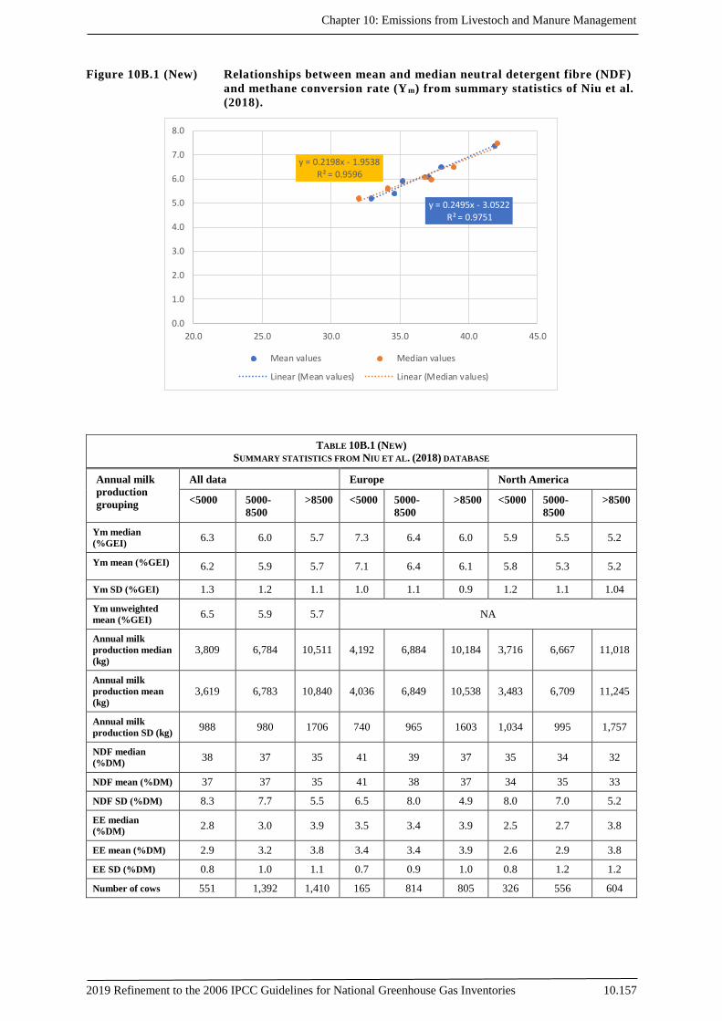
Chapter 10: Emissions from Livestoch and Manure Management
2019 Refinement to the 2006 IPCC Guidelines for National Greenhouse Gas Inventories 10.157
Figure 10B.1 (New) Relationships between mean and median neutral detergent fibre (NDF)
and methane conversion rate (Ym) from summary statistics of Niu et al.
(2018).
TABLE 10B.1 (NEW)
SUMMARY STATISTICS FROM NIU ET AL. (2018) DATABASE
Annual milk
production
grouping
All data Europe North America
<5000 5000-
8500
>8500 <5000 5000-
8500
>8500 <5000 5000-
8500
>8500
Ym median
(%GEI) 6.3 6.0 5.7 7.3 6.4 6.0 5.9 5.5 5.2
Ym mean (%GEI) 6.2 5.9 5.7 7.1 6.4 6.1 5.8 5.3 5.2
Ym SD (%GEI) 1.3 1.2 1.1 1.0 1.1 0.9 1.2 1.1 1.04
Ym unweighted
mean (%GEI) 6.5 5.9 5.7 NA
Annual milk
production median
(kg)
3,809 6,784 10,511 4,192 6,884 10,184 3,716 6,667 11,018
Annual milk
production mean
(kg)
3,619 6,783 10,840 4,036 6,849 10,538 3,483 6,709 11,245
Annual milk
production SD (kg) 988 980 1706 740 965 1603 1,034 995 1,757
NDF median
(%DM) 38 37 35 41 39 37 35 34 32
NDF mean (%DM) 37 37 35 41 38 37 34 35 33
NDF SD (%DM) 8.3 7.7 5.5 6.5 8.0 4.9 8.0 7.0 5.2
EE median
(%DM) 2.8 3.0 3.9 3.5 3.4 3.9 2.5 2.7 3.8
EE mean (%DM) 2.9 3.2 3.8 3.4 3.4 3.9 2.6 2.9 3.8
EE SD (%DM) 0.8 1.0 1.1 0.7 0.9 1.0 0.8 1.2 1.2
Number of cows 551 1,392 1,410 165 814 805 326 556 604
y = 0.2495x - 3.0522R² = 0.9751
y = 0.2198x - 1.9538
R² = 0.9596
0.0
1.0
2.0
3.0
4.0
5.0
6.0
7.0
8.0
20.0 25.0 30.0 35.0 40.0 45.0
Mean values Median values
Linear (Mean values) Linear (Median values)

Volume 4: Agriculture, Forestry and Other Land Use
10.158 2019 Refinement to the 2006 IPCC Guidelines for National Greenhouse Gas Inventories
TABLE 10B.2 (NEW)
THRESHOLD CALCULATION BASED ON NDF CORRECTION.
NDF Mean Median
32 5.08 4.93
33 5.30 5.18
34 5.52 5.43
35 5.74 5.68
36 5.96 5.93
37 6.18 6.18
38 6.40 6.43
39 6.62 6.68
40 6.84 6.93
In the case of beef cattle, a total of 113 measurements were compiled from 35 studies. Studies were divided by
their dominant diet type into three categories, high forage diets, mixed diets (mixed forage and concentrate) and
feedlot diets. Summary statistics were compiled and group averages are reported. Due to the variability in the data,
values were rounded based on expert judgement. An overall average was developed for the feedlot and non-feedlot
diets. Non feedlot diets were differentiated between dominantly forage based diets and mixed concentrate diets.
There is important variability in the results of studies that attempt to develop relationships between feed quality
and methane yield. Nonetheless, numerous empirical and biochemical modelling studies demonstrate both the
statistical significance and the biochemical processes that relate reductions in methane production with the
introduction of concentrates to ruminant diets (Mills et al. 2001; Mills et al. 2003; Ellis et al. 2006; Ellis et al.
2007; Ellis et al. 2009; Ellis et al. 2010; Alemu et al. 2011; Bannink et al. 2011; Ellis et al. 2014; Escobar-
Bahamondes et al. 2016; Kebreab et al. 2016). For this reason, methane conversion rates are produced from a
summary of low, medium and high dietary forage proportions. Raw data used in the development of these values
can be requested from the IPCC.
TABLE 10B.3 (NEW)
SUMMARY OF DATA COMPILED FOR THE COMPILATION OF YM VALUES FOR CATTLE AND BUFFALO
Category Measurement method
Average
Body
Weight (kg)
Methane yield
(g/kg DMI)
SD
(±)
Ym (%
GEI) SD (±) n
High forage
Chambers (24)
SF6 (30), Micro-
meteorological (2)
451 23.0 4.6 7.21 1.5 56
Intermediate
forage Chambers (17) SF6 (7) 401 21.0 3.8 6.3 1.2 24
Feedlot (low
forage)
Chambers (11) SF6 (5) Head
boxes (17) 450 12.99 3.3 3.842 1.0 33
Boadi and Wittenberg (2002); Pinares-Patiño et al. (2003); Boadi et al. (2004); Beauchemin and McGinn (2005); Beauchemin and McGinn
(2006a); Beauchemin and McGinn (2006b); Chaves et al. (2006); Doreau et al. (2011); Jordan et al. (2006a); Jordan et al. (2006b); Lovett
et al. (2003); Beauchemin et al. (2007); Hegarty et al. (2007); Hart et al. (2009); McGinn et al. (2009); Mc Geough et al. (2010a); Mc Geough et al. (2010b); Doreau et al. (2011); Hales et al. (2012); Kennedy and Charmley (2012); Staerfl et al. (2012); Chung et al. (2013);
Hünerberg et al. (2013a); Hünerberg et al. (2013b); Fiorentini et al. (2014); Hales et al. (2014); Hales et al. (2015); Romero-Perez et al.
(2014); Troy et al. (2015); Romero-Perez et al. (2015); Nascimento et al. (2016); Vyas et al. (2016a); Vyas et al. (2016b); Baron et al.
(2017); Hales et al. (2017). 1 Rounded to 7.0 for Table 10.12
2 Rounded to 4.0 for Table 10.12.

Chapter 10: Emissions from Livestoch and Manure Management
2019 Refinement to the 2006 IPCC Guidelines for National Greenhouse Gas Inventories 10.159
10B.3 Estimation of Default Emission Factor(s) for Goat Tier 2
parameters
A database was compiled from peer-reviewed articles that studied in-vivo methane (CH4) production from goat
enteric fermentation and N excretion. These studies were identified through a comprehensive literature search
performed in Goggle scholar and researchgate and from sources that carried out review work such as a recent study
attempting to derive statistical models for prediction of enteric CH4 from goats (Patra & Lalhriatpuii 2016) and a
New Zealand technical report for CH4 and N excretion rates for goats (Lassey 2012). Data were directly extracted
from the individual studies identified. Authors were contacted in order to fill in gaps of information from the
studies.
Overall, 63 publications were obtained from a varied sample of countries and 18 different goat breeds (Aguilera
et al. 1990; Prieto et al. 1990; Shibata et al. 1992; Haque et al. 1997; AFRC 1998; Haque et al. 1998; Islam et al.
2000; Islam et al. 2001; Rapetti et al. 2002; Puchala et al. 2005; Rapetti et al. 2005; Tovar-Luna et al. 2007b;
Tovar-Luna et al. 2007c; Tovar-Luna et al. 2007a; Animut et al. 2008; Bhatta et al. 2008; Haque et al. 2008;
Vermorel et al. 2008; Li et al. 2010; López et al. 2010a; López et al. 2010b; Tovar-Luna et al. 2010b; Tovar-Luna
et al. 2010a; Gerber et al. 2011; López et al. 2011; Tovar-Luna et al. 2011; Abecia et al. 2012; Jeong et al. 2012;
Lassey 2012; López et al. 2012; Mitsumori et al. 2012; Puchala et al. 2012a; Puchala et al. 2012b; Romero-Huelva
et al. 2012; Yang et al. 2012; Bhatta et al. 2013; Chethan et al. 2013; López & Fernández 2013; Martínez-
Fernández et al. 2013; Miri et al. 2013; López et al. 2014; Martínez-Fernández et al. 2014; Nielsen et al. 2014;
Romero-Huelva & Molina-Alcaide 2014; Ibáñez et al. 2015a; Ibáñez et al. 2015b; Lu et al. 2015; Wang & Xue
2015; Arif et al. 2016; Castro-Lima et al. 2016; Criscioni & Fernández 2016; Lu et al. 2016; Patra & Lalhriatpuii
2016; Wang et al. 2016a; Wang et al. 2016b; Arco-Pérez et al. 2017; Barbosa et al. 2017; Keli et al. 2017; Kumar
et al. 2017; Na et al. 2017; Romero-Huelva et al. 2017; Tovar-Luna et al. 2017; Azlan et al. 2018; Fernández et al.
2018; Li et al. 2018b; Na et al. 2018a; Na et al. 2018b; Puchala et al. 2018)
Although there was a total of 290 treatment means, treatments that were using substances with antimethanogenic
properties were excluded before analysis. The minimum prerequisite for a study to be included in the data set was
that Ym values (or gross energy and CH4 output energy) were reported.
Information on feed and diet characteristics, feed intake, breed, animal type, digestibility, and rumen were
collected in the final data set. Table 10B.4 shows the mean and the range of some of the diet and animal variables
for the different studies. Values were quite heterogeneous. For example, dry matter intake ranged between 0.14
and 2.51 kg DM intake/day animal (0.93 on average).
The concentrations of crude protein (CP), neutral detergent fibre (NDF) and starch were within the range of 6-26
percent (mean value of 15 percent), 18-74 percent (mean value of 42 percent) and 1-42 percent (mean value of 19
percent), respectively.
Methane production was expressed as grams per day, liters per day, megajoules per day, or as a proportion of GE
or DE; therefore, the following factors were used in converting units: 1 g = 1.40 L =55.5 kJ; 1 L = 0.716 g = 39.54
kJ.
TABLE 10B.4 (NEW)
MEAN, MEDIAN, MAXIMUM, MINIMUM AND QUARTILE 1 AND 3 (Q1 AND Q3) VALUES FOR A SELECTION FEED DIET
COMPOSITION, FEED INTAKE, BODY WEIGHT AND MILK PRODUCTIVITY.
Digestibility (%) Feed intake body
weight
Milk
yield
DM OM N NDF GE DM
(kg/day)
GE
(MJ/day)
DE
(MJ/day) kg/animal
(kg/day
animal)
Mean 68% 69% 72% 54% 71% 0.94 18.77 12.18 39.82 1.90
Median 69% 71% 73% 53% 72% 0.78 15.20 9.44 40.05 1.59
Max 83% 91% 84% 82% 83% 2.59 46.68 29.90 64.00 3.69
Min 49% 40% 44% 18% 52% 0.14 4.64 6.02 14.53 0.81
Q1 64% 65% 67% 46% 67% 0.62 11.80 8.44 33.45 1.31
Q3 74% 76% 78% 60% 76% 1.14 26.12 11.09 47.55 2.28
The CH4 emissions also varied greatly in the dataset. Table 10B.5 shows the methane emissions expressed in
different units and metrics.

Volume 4: Agriculture, Forestry and Other Land Use
10.160 2019 Refinement to the 2006 IPCC Guidelines for National Greenhouse Gas Inventories
TABLE 10B.5 (NEW)
MEAN, MEDIAN, MAXIMUM, MINIMUM AND QUARTILE 1 AND 3 (Q1 AND Q3) VALUES FOR CH4
PRODUCTION RESULTS REFERRED AS A PROPORTION OF GROSS ENERGY INTAKE (CH4
CONVERSION FACTOR: YM), DAY-1, KG DM INTAKE-1, KG OF MILK PRODUCED-1 AND KG OF BODY
WEIGHT-1
CH4
Ym MJ/day MJ/kg DM MJ/kg milk J/kg BW
Mean value 5.3% 0.9 1.0 0.8 23.1
Median 5.3% 0.8 1.0 0.8 20.5
Max 10.3% 3.8 4.7 1.7 73.6
Min 1.2% 0.2 0.3 0.2 5.3
Q1 4.3% 0.6 0.8 0.6 15.8
Q3 6.3% 1.0 1.2 1.1 27.4
The average methane emission was 16.2 g CH4/animal day, 18.3 g CH4/kg DM intake, 0.42 g CH4/ kg BW (data
not shown). Average/median methane conversion factor (Ym) was 5.3 percent, which is in the range of the recent
value obtained by the study by Patra & Lalhriatpuii (2016), which included 42 studies.
We analyzed the relationship between methane output and diet type (e.g. diet digestibility, percent forage use) but
there were not any clear statistical relationships between diet type and enteric methane output (data not shown).
In general increased body weight and milk yield resulted in greater CH4 output but body weight and milk yield did
not show any statistical relationship with Ym (data not shown).
Methane output per animal were positively correlated with dry matter (Fig 10A.10) and gross energy (Fig 10A.11)
intake (R2=0.60; P<0.00001).
Figure 10B.2 (New) Annual enteric methane output per animal expressed in mass in
relation to daily dry matter (DM) intake.

Chapter 10: Emissions from Livestoch and Manure Management
2019 Refinement to the 2006 IPCC Guidelines for National Greenhouse Gas Inventories 10.161
Figure 10B.3 (New) Daily enteric methane output per animal expressed in energy in
relation to daily gross energy (GE) intake.
In order to develop Tier 1 EF for enteric CH4 from goats for both low and high production systems the following
steps were followed: Average goat weight (LW) for high and low production systems were estimated using global world information
from Gerber et al. (2013). For high and low production systems it was estimated average weight values of 50 kg
and 28 kg, respectively.
Daily dry matter intake per animal was estimated as a function of animal weight using the equation from AFRC
(1998).
Using the equation from Fig 1 we obtained kg CH4/animal yr as a function of the previously estimated value of
daily dry matter intake.
EF for Tier 1 resulted in 8.7 and 4.9 kg CH4/head yr for high and low production systems, respectively. These
values are both lower than that estimated than Vermorel et al. (2008) from French systems (11.9 kg CH4/head yr-
1) and that from high production systems is similar to that proposed for Lassey ( 2012) for New Zealand goat herd.
Considering the data analysed, a Ym methane conversion factor a 5.5 percent has been chosen. No clear evidence
was found to develop Ym factors separately as a function of diet quality or production system.
In order to develop default values for N excretion rates (for Table 10.19) the following steps were followed:
Average goat weight (LW) for each global region were estimated using global world information from GLEAM
FAO.
Daily N intake per animal and day was estimated as a function of average goat weight using the relationship
developed from this database relating goat weight and N intake (Fig 10B.3-3) (R2=0.48; P<0.00001).
Daily N excretion rate was subsequently calculated using the relationship also found using this database relating
daily N intake and daily N excretion (Fig 10B.4-4) (R2=0.89; P<0.00001) and transforming values to excretion
rates espressed as kg N (1000 kg animal mass)-1) day-1.
Figure 10B.4 (New) Daily N excretion output per animal expressed in relation to animal
weight.

Volume 4: Agriculture, Forestry and Other Land Use
10.162 2019 Refinement to the 2006 IPCC Guidelines for National Greenhouse Gas Inventories
Figure 10B.5 (New) Daily N excretion output per animal expressed in relation to daily N
intake.
In order to develop default values for volatile solids (VS) excretion rates (for Table 10.14A) we calculated daily
VS excretion from goats for each world region according to equation 10.24. Gross energy intake was estimated
from previously calculated DM intake for Tier1 EF for enteric CH4 and the conversion factor for dietary GE (18.45
MJ/kg DM). We assumed that digestibility of the feed was 50 and 60 percent for developing and developed
countries, respectively. The ash content of the feed was assumed to be 8 percent. We assumed the animal weights
for each region based on information from FAO work: GLEAM FAO.

Chapter 10: Emissions from Livestoch and Manure Management
2019 Refinement to the 2006 IPCC Guidelines for National Greenhouse Gas Inventories 10.163
10B.4 Feed intake estimates using a simplified Tier 2 method
Prediction of DMI for catt le based on body weight and estimated dietary net energy
concentration (NEm a) or digestible energy values (DE percent):
Several studies have shown that dry matter intake (DMI) is highly and positively related to methane emissions. In
some cases it has been reported that up to 92 percent of the variability in enteric methane emissions could be
explained by DMI alone (Charmley et al. 2016). Most models developed to predict enteric methane emissions
usually include either DMI or some form of feed intake. There are a number of models already developed with the
objective of predicting DMI and these could be used in conjunction with emission factors to estimate enteric
methane emissions in a Tier 2 approach. Appuhamy et al. (2016) evaluated 40 prediction equations using data that
included measured DMI and feed quality attributes from North America, Europe and Australia/New Zealand. The
best performing models in each region were then re-evaluated using calculated DMI and compared with estimates
that used measured DMI. They evaluated several DMI prediction equations including the Cornell Net
Carbohydrate and Protein System (CNCPS, Fox et al. 1992) as modified by Arnerdal (2005), National Research
Council (NRC 2001) (developed based on North America cows), Lindgren et al. (2001) and Arnerdal (2005)
(developed using data from cows in Europe), and Vazquez and Smith (2000) model (developed from
Australia/New Zealand data). Appuhamy et al. (2016) reported that models using estimated DMI predicted enteric
methane emissions just as good as the measured data and concluded that enteric methane emissions from dairy
cows can be predicted successfully with estimated DMI, particularly using the modified CNCPS model.
Appuhamy et al. (2018) further evaluated the comprehensive (IPCC-CMP) and simplified (IPCC-SMP) IPCC
models (IPCC 2006) to predict DMI as well as the modified CNCPS and NRC (2001) models to predict DMI using
an independent data. The modified CNCPS relying on BW and fat corrected milk yield (Eq. 1) more accurately
predicted DMI (RMSPE = 14.1 percent) than NRC (RMSPE = 19.4 percent), IPCC-SMP (RMSPE = 16.9 percent),
and IPCC-CMP (RMSPE = 23.4 percent). Overall, the results demonstrated that DMI of dairy cows can be
predicted successfully using information such as milk yield, milk fat content, and body weight (BW) that are
routinely available in dairy farms.
DMI (kg/d) = 0.0185 x BW (kg) + 0.305 x fat corrected milk (kg/d) Eq [1]
A simplified approach can also be used to estimate DMI of beef cattle, updated based on the most recent
methodologies as described by NASEM (2017). For growing and finishing cattle, equations are:
Calves
DMI (kg/d) = (BW0.75 x (0.2435 x NEm – 0.0466 x NEm2 – 0.1128)) / NEm Eq. [2]
Yearlings
DMI (kg/d) = (BW0.75 x (0.2435 x NEm – 0.0466 x NEm2 – 0.0869)) / NEm Eq. [3]
Feedlot cattle (high grain diets)
Steers: MI (kg/d) = 3.830 + 0.0143 x BW x 0.96 Eq. [4]
Heifers: DMI (kg/d) = 3.184 + 0.01536 x BW x 0.96 Eq. [5]
Where: BW = body weight (kg), NEm = Mcal/kg feed DM Eq. [6]
Mature Cows
Forage type Digestibility Forage DMI Capacity (kg/day), % of BW (kg)
Non-lactating Lactating
Low quality <52 1.8 2.2
Average quality 52-59 2.2 2.5
High quality >59 2.5 2.7

Volume 4: Agriculture, Forestry and Other Land Use
10.164 2019 Refinement to the 2006 IPCC Guidelines for National Greenhouse Gas Inventories
10B.5 Basis for Changes to MCF Calculations for Liquid/Slurry
The following briefly summarizes the 2006 approach and improvements included in the current approach.
IPCC 2006 Model for Liquid/Slurry:
The IPCC 2006 MCF for liquid slurry was based on the following relationship:
MCF = f
where f was calculated with the following temperature-dependent Arrhenius function, derived from Mangino et
al., 2001, which is based on Safley & Westerman (1990):
f = EXP[(Ea×(T2-T1))/(R×T2×T1)]
where,
f is a dimentionless fraction (0 to 1). Originally, Safley & Westerman (1990) used f to design an anaerobic digestion
system at a lower temperature (T2) based on known performance of a digester at a warmer temperature (T1).
Ea is the activation energy. Originally, Safley and Westerman used Ea = 15175 cal/mol, based on an earlier study.
Mangino et al. 2001 continued to use 15175 cal/mol.
T2 is the variable temperature (K). Defined by Safley & Westerman (1990) as the unknown anaerobic digester
temperature. Mangino et al. 2001 defined T2 as the monthly temperature of the anaerobic lagoon (assuming
equality with monthly average air temperature). IPCC (2006) defined T2 as the annual average temperature of a
region.
T1 is the reference temperature (K). Defined by Safley & Westerman (1990) as 30 °C (303.16 K). Mangino et al.
2001 and IPCC 2006 use the same value.
R is the gas constant 1.987 cal k-1 mol-1.
The reasons for modification of MCF, though the Methane conversion factor
(MCF) remains an uncertain parameter.
First and foremost, in the IPCC 2006 , the MCF parameter violates a first-principle of inventory development:
comparability. The use of an annual average temperature to calculate MCF systematically underestimates the
annual MCF due to the mathematical principle known as Jensen’s Inequality which applies to non-linear functions
such as the Arrhenius equation (VanderZaag et al. 2018). Using this mathematical principle it can be shown that
for a 1-month retention time, the annual average MCF calculated based on monthly temperature will always exceed
the MCF calculated from the annual average temperature. Therefore, the IPCC 2006 MCF values are
underestimates, and the level of underestimation is greatest for countries with large seasonal temperature extremes.
The 2006 model also used an MDP factor which reduced the mass of VS entering the manure storage or lagoon.
Since VS cannot simply vanish, there needs to be justification for altering the VS loading rate. In the modified
method, the MCF calculation used an MDP = 1.0, which means we are assuming the VS Excretion rates are correct,
and that VS Excreted enters the liquid manure storage. MDP factors may be used in specific cases such as when
solid-liquid separation systems are used, whereby VS is removed from the liquid system and transferred to a solid
system. However in most cases the use of MDP factor is indicative of an inaccurate B0 or VS input into the manure
storage system.
For the sake of completeness, it is worth pointing out that the quantity of VS entering liquid storage could be
greater than VS excreted (implied MDP >1.0). For instance, the use of straw bedding results in additional VS
entering the liquid storage. Another example is waste milk (from treated cows, or from cleaning milking systems)
on dairy farms which adds VS to the storage. Secondly, it is well known that the retention time of liquid manure
in storage is a critical parameter in determining MCF, and the 2006 IPCC Guidelines state “both temperature and
retention time play an important role in the calculation of MCF”. However, the IPCC 2006 calculations of MCF
(Table 1), give very little focus to retention time. Previous IPCC Good Practice Guide recommended that future
MCFs be modeled accounting for the storage period (Zeeman & Gerbens 2000). Furthermore, the work of Safley
& Westerman (1990) showed that the same amount of VS destruction can be achieved by longer retention time at
lower temperature compared with shorter retention time at higher temperature. Furthermore the suggestion to use
equation 1 for batch-fed storage/digesters that is currently in 2006 IPCC Guidelines would not result in a value
that is comparable to the default annual temperature values, because this equation would inherently require
inclusion of retention time.

Chapter 10: Emissions from Livestoch and Manure Management
2019 Refinement to the 2006 IPCC Guidelines for National Greenhouse Gas Inventories 10.165
Recent year-round field studies in climates where the annual average air temperature was <10°C have reported
MCFs in the range of 0.61 (Wightman & Woodbury 2016) , ≥0.57 (Balde et al. 2016a) at liquid dairy manure
storages, and greater for anaerobic lagoons (Leytem et al. 2017). Controlled studies at or around 20°C without
added inoculum reported MCF of 55 percent over 165 d (VanderZaag et al. 2010) and 32 percent over 150-d
(Masse et al. 2008). Another study showed the MCF increased non-linearly with the duration of storage (Le Riche
et al. 2016). Previous IPCC Guidance reported an MCF of 39 percent, 45 percent, and 72 percent for liquid/slurry
for Cool, Temperate, and Warm climates, respectively (Zeeman & Gerbens 2000). They also stated that
liquid/slurry storage tanks were considered to have ≥6 month retention time. Therefore, the interaction between
retention time and temperature has long been recognized, but the calculation of MCFs has not been fully
transparent about how this important interaction has been handled (or how it should be handled by practitioners)
and therefore has made comparability with measurements challenging.
Thirdly, the single temperature time step given in the IPCC guidelines suggests a level of certainty that is simply
not supported by the experimental results, considering the approach being used.
TABLE 10B.6 IPCC 2006 TABLE OF MCF VALUES FOR LIQUID/SLURRY (TABLE 10.17)
Proposed Changes:
The proposed change is to use a spreadsheet model to calculate MCF using monthly temperature in each IPCC
climate region, and for a specific liquid manure retention time (e.g. the Table below). Therefore, this approach
produces MCF values that account for both temperature and retention time, while leaving the users to decide which
retention time is appropriate for their manure management systems. The spreadsheet model will be made available
as well.
TABLE 10B.7 (NEW)
MCFS CALCULATED FOR EACH RETENTION TIME AND CLIMATE. (SELECTED IPCC CLIMATE REGIONS SHOWN)
Tropical
Montane
Tropic
al1 Wet
Tropical1
Moist
Tropical1 Dry
Warm Temperate
Moist
Warm
Temperate Dry
Cool Temperate
Moist
Cool
Temperate Dry
RETENTIO
N TIME N_TM
N_T
W
N_TM
st
N_T
D N_WTM N_WTD N_CTM N_CTD
1 Month 0.25 0.38 0.36 0.42 0.13 0.15 0.06 0.08
3 Month 0.43 0.61 0.57 0.62 0.24 0.28 0.12 0.16
4 Month 0.50 0.67 0.64 0.68 0.29 0.32 0.15 0.19
6 Month 0.59 0.76 0.73 0.74 0.37 0.41 0.21 0.26
12 Month 0.73 0.80 0.80 0.80 0.55 0.64 0.31 0.42
Tavg C 21.5 25.9 25.2 25.6 13.9 14.0 4.6 5.8
1 Note that an upper limit mcf of 80% has been imposed for consistency with the anaerobic lagoon mcfs at high temperatures and long
retention times
Changes in l iquid/slurry MCF, compared to the IPCC 2006 are summarized below:
#1 – Timestep:
Monthly temperature (proposed) instead of annual average temperature (IPCC 2006)

Volume 4: Agriculture, Forestry and Other Land Use
10.166 2019 Refinement to the 2006 IPCC Guidelines for National Greenhouse Gas Inventories
Methane emissions are non-linearly related to temperature, therefore Jensen’s inequality states that the use of the
average temperature will lead to systematic underestimation. As a result, monthly average air temperature is
proposed for the calculation of MCF, rather than annual average temperature. Therefore, it is proposed that MCF
for liquid/slurry be calculated using the Mangino et al. (2001) spreadsheet model, with the regional climate data
from the IPCC defined climate regions. Additional details below.
#2 – Retent ion Time:
Several retent ion t imes (proposed) instead of 1 -month impl ied retention t ime ( IPCC
2006)
Retention time is a crucial parameter determining the extent of methane emissions and the quantity of VS in storage
at any given time, therefore affecting the MCF. The IPCC 2006 used a 1-month retention time for all liquid/slurry
systems by using MCF = f, based on an annual average temperature. Using a 1-month retention time is unrealistic,
since the majority of liquid/slurry storages are meant for storage over several months or more. Therefore, it is
proposed to calculate MCF based on five retention times: 1 month, 3 months, 4 months, 6 months, and 12 months.
Proposed “Good Practice” in the case of countries that do not know have information on retention times is to use
the six month retention time.
#3 – Act ivation Energy (Ea):
Updated Ea va lue (19347 cal/mol proposed) instead of 15175 ca l /mol (IPCC 2006)
Recent research from Petersen et al. (2016) and Elsgaard et al. (2016) propose a new Ea value of 81 kJ/mol =
19347 cal/mol. It is proposed to use this updated value.
#4 – Reference Temperature (T 1) :
Updated T1 va lue (308.16 proposed) instead of 303.16 K (IPCC 2006)
The value of T1 used by IPCC 2006 and Mangino et al. (2001) is directly taken from Safley & Westerman (1990).
The original intent of Safley and Westerman was comparing performance of a known and unknown anaerobic
digester performance. In Mangino et al. (2001) and IPCC (2006) the value of T1 defines the temperature at which
f = 1.0, therefore T1 defines the temperature at which the B0 will be reached in one month. There is considerable
literature on laboratory methods for incubating manure to measure methane potential (e.g. BMP, B0) and it is
customary for the temperature of these incubations to be ca. 35°C, rather than 30°C. With a temperature of 35°C
it would be reasonable to expect the B0 to nearly be reached in 30 days (i.e. one month) (e.g. Owen et al. 1979;
Pham et al. 2013). Therefore, it is proposed to change T1 to 308.16 K (=35 + 273.16).
#5 – Manure Temperature (T 2) :
Manure temperature lagging behind T a i r (proposed) instead of equal T a i r ( IPCC 2006)
Most of the time, manure temperature does not equal air temperature. The temperature of liquid manure tends to
lag behind air temperature. While models for manure temperature do exist (Rennie et al. 2017) this is too complex
for the general guidelines. As a pragmatic alternative, a 1-month lag is proposed, i.e., set T2 = Tair from the previous
month. It has also been shown (Rennie et al. 2018) that manure storages which are emptied once per year at the
end of the growing season before winter stay cooler than air temperature during the summer. Therefore, only in
the case of once per year emptying (i.e. 12 month retention time), a downward temperature shift of 3°C has also
been applied.
#6 – VS carryover after emptying:
After manure is removed, 5 percent remains (proposed), instead of complete emptying
(IPCC 2006)
It has been shown in several studies that farms do not completely empty liquid/slurry storages due to the practical
challenge of doing so at the farm-scale (Balde et al. 2016b). Therefore, it is proposed that 5 percent of VS is
retained in storage after emptying, rather than 0 percent (i.e. completely clean) assumption implied in the IPCC
2006 calculations. It is noteworthy that the IPCC 2000 Good Practice Guide (Zeeman & Gerbens 2000) mention
approximately 15 percent of the manure storage cannot be emptied.
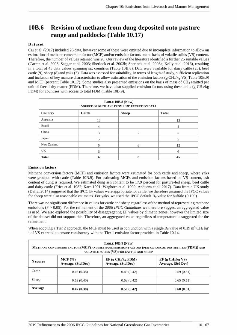
Chapter 10: Emissions from Livestoch and Manure Management
2019 Refinement to the 2006 IPCC Guidelines for National Greenhouse Gas Inventories 10.167
10B.6 Revision of methane from dung deposited onto pasture
range and paddocks (Table 10.17)
Dataset
Cai et al. (2017) included 26 data, however some of these were omitted due to incomplete information to allow an
estimation of methane conversion factor (MCF) and/or emission factors on the basis of volatile solids (VS) content.
Therefore, the number of values retained was 20. Our review of the literature identified a further 25 suitable values
(Carran et al. 2003; Saggar et al. 2003; Sherlock et al. 2003b; Sherlock et al. 2003a; Kelly et al. 2016), resulting
in a total of 45 data values spanning six countries (Table 10B.8). Data were available for dairy cattle (25), beef
cattle (9), sheep (8) and yaks (3). Data was assessed for suitability, in terms of length of study, sufficient replication
and inclusion of key manure characteristics to allow estimation of the emission factors (g CH4/kg VS; Table 10B.9)
and MCF (percent; Table 10.17). Some studies also presented emissions on the basis of mass of CH4 emitted per
unit of faecal dry matter (FDM). Therefore, we have also supplied emission factors using these units (g CH4/kg
FDM) for countries with access to total FDM (Table 10B.9).
TABLE 10B.8 (NEW)
SOURCE OF METHANE FROM PRP EXCRETION DATA
Country Cattle Sheep Total
Australia 13 13
Brazil 4 4
China 3 2 5
Japan 5 5
New Zealand 6 6 12
UK 6 6
Total 37 8 45
Emission factors
Methane conversion factors (MCF) and emission factors were estimated for both cattle and sheep, where yaks
were grouped with cattle (Table 10B.9). For estimating MCFs and emission factors based on VS content, ash
content of dung is required. We estimated dung ash content to be 17.9 percent for pasture-fed sheep, beef cattle
and dairy cattle (Fries et al. 1982; Karn 1991; Waghorn et al. 1999; Andueza et al. 2017). Data from a UK study
(Defra, 2014) suggested that the IPCC B0 values were appropriate for cattle, we therefore assumed the IPCC values
for sheep were also reasonable estimates. For yaks, we used the IPCC default B0 value for buffalo (0.100).
There was no significant difference in values for cattle and sheep regardless of the method of representing methane
emissions (P > 0.05). For the refinement of the 2006 IPCC Guidelines we therefore suggest an aggregated value
is used. We also explored the possibility of disaggregating EF values by climatic zones, however the limited size
of the dataset did not support this. Therefore, an aggregated value regardless of temperature is suggested for the
refinement.
When adopting a Tier 2 approach, the MCF must be used in conjunction with a single B0 value of 0.19 m3 CH4 kg-
1 of VS excreted to ensure consistency with the Tier 1 emission factor provided in Table 10.14.
TABLE 10B.9 (NEW)
METHANE CONVERSION FACTOR (MCF) AND METHANE EMISSION FACTORS (PER KG FAECAL DRY MATTER (FDM)) AND
VOLATILE SOLIDS (VS) FOR CATTLE AND SHEEP
N source MCF (%)
Average, (Std Dev)
EF (g CH4/kg FDM)
Average, (Std Dev)
EF (g CH4/kg VS)
Average, (Std Dev)
Cattle 0.46 (0.38) 0.49 (0.42) 0.59 (0.51)
Sheep 0.52 (0.40) 0.53 (0.42) 0.65 (0.51)
Average 0.47 (0.38) 0.50 (0.42) 0.60 (0.51)

Volume 4: Agriculture, Forestry and Other Land Use
10.168 2019 Refinement to the 2006 IPCC Guidelines for National Greenhouse Gas Inventories
10B.7 Estimation of default emission factors for MCF CH4
values, EF for direct N2O emissions, NH3, NO3 leaching
and N2 emissions from solid storage and composting
systems
Methodolog ies
The estimation of updated MCF values, EF for direct N2O emissions and NO3 leaching and N2 from both (i) solid
storage and (i) two composting systems (static pile and passive windrow) are based on an extensive meta-analysis
of 50 peer-reviewed research articles involving 304 observations and published in open access by Pardo et al.
(2015). In this study it was quantified the response of GHG emissions, NH3 emissions, and total N losses to
different solid waste management strategies (conventional solid storage, turned composting, forced aerated
composting, covering, compacting, addition/substitution of bulking agents and the use of additives).
For solid storage, new treatments have been proposed to be incorporated in the 2019 Refinement:
covering/compacted (both treatments had similar effects on GHG emissions), addition/substitution of bulking
agents and the use of additives. In the 2006 IPCC Guidelines for National GHG inventories default emission
factors for solid storage were based on expert IPCC judgement and a single study (Amon et al. 2001). In Pardo et
al. (2015) the estimation of MCF values and EF for direct N2O emissions from solid storage (without treatment)
is based on data from 30 studies at the farm level.
For the new treatments, MCF values and EF for direct N2O emissions have been based on:
9 studies for compacting and covering;
11 studies for addition/substitution of bulking agents;
6 studies for use of additives.
For the rest of the management systems, MCF values and EF for direct N2O emissions have been based on:
22 studies for solid storage;
6 studies for composting-static piles (Forced aeration);
11 studies for composting-Passive windrow (infrequent turning).
Based on the IPCC (2006) climate zone classification two factors were defined: Temperature, which involved two
categories (i) Warm temperate and (ii) Cool temperate; and annual rainfall rate, including (i) Dry, (ii) Moist and
(iii) Wet conditions.
CH 4 MCF
For the absolute values of CH4 values, Pardo et al. (2015) used untreated solid storage as a reference system. They
compared estimated percent C lost as CH4 using the IPCC (2006) method (IPCC 2006 MCF) with the values
obtained at the different studies (Figure 10B.6).

Chapter 10: Emissions from Livestoch and Manure Management
2019 Refinement to the 2006 IPCC Guidelines for National Greenhouse Gas Inventories 10.169
Figure 10B.6 (New) Comparison between ranges of CH4-C emissions observed in collected
studies in Pardo et al. (2015) (new) with estimations for the same
studies according to IPCC (2006) methodology. Figure adapted from
Pardo et al. (2015).
For untreated solid storage systems Pardo et al. (2015) showed that overall values were within the IPCC (2006)
range for CH4 emissions (Figure 10B.6) and confirmed that the differences between cold and temperate conditions
were in agreement with those indicated by IPCC (2006) not shown here, Figure S3b in Pardo et al. (2015). There
were not enough studies under warm conditions and therefore, the assumption is to keep the same values indicated
by IPCC (2006).
Values for new solid storage treatments and composting (static pile and passive windrow) are estimated using the
reference value from the untreated solid storage system and the relative differences observed in Pardo et al. (2015).
For the new treatments, covering or compacted solid storage resulted in emissions in the same range as in solid
storage not shown here, Figure 2b in Pardo et al. (2015) and estimated reduction of 75 percent and 50 percent was
observed due to bulking agent addition and additives, respectively not shown here, Figure 2b in Pardo et al. (2015).
The differences amongst climatic zones were assumed to be in the same proportion as that found for untreated
solid storage systems.
Both composted static piles and static windrows were estimated to produce 50 percent of the CH4 coming from
solid storage not shown here, Figure 2b in Pardo et al. (2015), which results in consistently greater values than
those indicated by IPCC (2006). As a difference to IPCC (2006), CH4 emissions were found to be temperature
dependent for both composting systems (IPCC, 2006 did not indicate temperature differences for static piles).
N2O EF3 (Table 10.21)
According to the data examined in Pardo et al. (2015), there was no evidence to assume a lower EF for solid
storage systems (0.005 kg N2O–N kg−1 N excreted) than for passive windrow composting (0.01 kg N2O–N kg−1N
excreted). In fact, an EF of 0.5 percent (0.005kg N2O-N kg initial N-1) and 1 percent (0.01kg N2O-N kg initial N-
1) were found for composting-passive windrow and solid storage, respectively.
Composting static pile, in contrast to IPCC (2006), was found to emit greater N2O emissions than passive windrows
(not shown here, Fig. 3a in Pardo et al., 2015).
For the different treatments of solid storage, whereas Pardo et al. (2015) found no different effect on N2O after
compaction or covering, for both the addition of bulking agents or additives, a reduction of about 50 percent
compared with conventional solid storage was observed not shown here, Figure 2a in Pardo et al. (2015).
NH 3 losses
For solid storage and composting relative values compared to solid storage are trying to reflect results obtained
from meta-analysis by Pardo et al. (2015) (Fig 10A.15). Ammonia and NOx default values in Table 10.22 for
conventional solid manure storage and other categories present in both IPCC guidelines and EMEP/CORINAIR
guidelines have been taken from current EMEP/CORINAIR (2016). EMEP EF values, which are expressed per
TAN excreted and for each of the phases of the manure management, have been re-calculated to be expressed as

Volume 4: Agriculture, Forestry and Other Land Use
10.170 2019 Refinement to the 2006 IPCC Guidelines for National Greenhouse Gas Inventories
a funtion of total N excreted considering the mass balance flow between the different manure management phases
prior to manure application (housing, yards and storage). For other categories not present in EMEP/CORINAIR
(2016), first for stages prior to storage, we have estimated percent N lost using default EMEP/CORINAIR EFs for
conventional manure storage and assuming no N2O or N2 losses, and subsequently, during storage, we used the
relative effect between solid storage and the alternative solid storage categories (e.g. composting) (Fig 10A.15) as
the basis to estimate NH3+NOx EF during storage.
Figure 10B.7 (New) Effect on cumulative NH3-N emissions of different solid storage and
composting methods compared with conventional solid storage. Figure
adapted from Pardo et al. (2015)
NO 3 leaching and N 2 losses
Nitrate leaching/run-off has been estimated from the database from Pardo et al. (2015). For solid storage and
composting some of the studies included measurements of N leaching (15), some of which estimated N2 from the
total N balance, but only one included measurements of N2 (Moral et al. 2012). As a median value about 3 percent
is estimated to be lost as NO3 leaching/run-off (range: 0-38 percent). This value is subject to large uncertainty. In
fact these trials may not represent common practices where the efficiency of collection of excreta N is much lower
and can lead to as great as 50 percent losses (e.g. Lekasi et al. 2001; Rufino et al. 2007). Nitrogen (N2) losses, have
only been, to our knowledge, measured by Moral et al. (2012) (12 percent) and even though they could be estimated
as a result of an N balance from trials where all N flows expept N2 have been measured, the results are very
uncertain (0-55 percent). For N2, an estimated median value of 12 percent was found; coinciding with the measured
value by Moral et al. (2012), Systems that do not percolate but are subject to large water input will have greater
N2 losses and lower NO3 leaching-runoff. The opposite effect will be expected with rainy areas with no
containment and large possibilities for run-off/leaching. Values must be considered with large caution.
A further summary review was carried out to identify run-off/leaching values from dry lots and manure pack. As
observed in the 2006 IPCC Guidelines runoff and leaching values varied greatly citing ranges of 3 to 6 percent of
N excreted (Eghball & Power 1994) or 5 to 19 percent (Bierman et al. 1999). In humid environments losses can
be significant reaching 22-25 percent (Uusi-Kämppä 2002). However, uncovered holding and feeding pens without
runoff containment tend to be in drier climates simply due to challenges in moisture control in more humid
environments. Furthermore, considerable numbers of cattle are raised in drier climates and as a result considerably
more studies exist looking at runoff from feedlots and drylots. Likewise recent attempts have been made to attempt
to model these losses to the environment (Kizil et al. 2006; Williams et al. 2006). These studies tend to place the
range of runoff loss between 1 percent and roughly 7 (Kizil et al. 2006; Erickson & Klopfenstein 2010; Vadas &
Powell 2013). It is proposed the value of 3.5 percent with an uncertain range of 0 to 7 percent be considered as a
default leaching factor for open, uncovered, uncontained drylots and bedded pack to provide a Tier 1 estimate of
the fraction of N excreted lost to the environment.
Inventory compilers must be careful to consider that this refers to N lost to the environment surrounding the pens
or leached into the soil. If runoff is captured and returned to agricultural fields these losses must not be considered.
In humid environments, in cases where manure is left exposed to rainfall, inventory compilers should consider the
use of the upper bounds of the leaching fraction and furthermore to consider the development of a country specific
leaching fraction.
Review on the effect of slurry store so lid covers and natural crust in emissions of CH 4
and N 2 O

Chapter 10: Emissions from Livestoch and Manure Management
2019 Refinement to the 2006 IPCC Guidelines for National Greenhouse Gas Inventories 10.171
The review found 18 papers dealing with the impact of solid covers or natural crusts on CH4 and/or N2O emissions
from slurry stores.11 of them were suitable to be included here to deduce emission factors (Amon et al. 2006;
Clemens et al. 2006; Guarino et al. 2006; Amon et al. 2007; VanderZaag et al. 2008; VanderZaag et al. 2009;
Aguerre et al. 2012; Nielsen et al. 2013; Hou et al. 2015; Matulaitis et al. 2015; Misselbrook et al. 2016)
For CH4 emissions from Liquid/Slurry, the IPCC 2006 IPCC Guidelines state that by judgement of the IPCC
Expert Group, a reduction of 40 percent due to crust cover (40 percent) may be applied when a thick, dry, crust is
present. The new review carried our within the 2019 refinement confirms this judgement (VanderZaag et al. 2008;
Aguerre et al. 2012; Nielsen et al. 2013). A solid cover reduces CH4 emissions by 25 to 50 percent (range: 0 to 90
percent) (Amon et al. 2006; Clemens et al. 2006; Guarino et al. 2006; Amon et al. 2007; VanderZaag et al. 2008;
VanderZaag et al. 2009; Hou et al. 2015; Matulaitis et al. 2015; Misselbrook et al. 2016).
For N2O emissions from Liquid/Slurry with natural crust cover a detailed literature review carried out during the
2019 refinement revealed only very few new datasets on the measurement of N2O emissions from manure stores
and the influence of crusting. These datasets agree that N2O emissions increase when a crust is formed, but do not
give concrete numbers on the level of increase (VanderZaag et al. 2008; Aguerre et al. 2012).
For N2O emissions from Liquid/Slurry with a cover a detailed literature review carried out during the 2019
refinement revealed only few new datasets on the measurement of N2O emissions from manure stores. These
datasets emcompass a large range of N2O emissions from a 50 percent reduction to a 100 percent increase in N2O
emissions when slurry stores are covered. The 2019 refinement therefore suggest to use the emission factor of crust
cover (Amon et al. 2006; Clemens et al. 2006; Guarino et al. 2006; Amon et al. 2007; VanderZaag et al. 2009;
Hou et al. 2015; Misselbrook et al. 2016).

Volume 4: Agriculture, Forestry and Other Land Use
172 2019 Refinement to the 2006 IPCC Guidelines for National Greenhouse Gas Inventories
References
Section 10.2 Livestock Population and Feed
Characterisation
REFERENCES NEWLY CITED IN THE 2019 REFINEMENT
AFRC (1998) The Nutrition of Goats. Wallingford: CAB International. pp 118.
Animut G., Puchala R., Goetsch A.L., Patra A.K., Sahlu T., Varel V.H., Wells J. (2008) Methane emission by
goats consuming different sources of condensed tannins. Animal feed science and technology 144: 228-241.
Arnerdal S. (2005) Predictions for voluntary dry matter intake in dairy cows. Thesis. Department of Animal
Nutrition and Management, Swedish University of Agricultural Sciences.
Fox D.G., Sniffen C.J., Oconnor J.D., Russell J.B., Vansoest P.J. (1992) A Net Carbohydrate and Protein System
for Evaluating Cattle Diets .3. Cattle Requirements and Diet Adequacy. Journal of Animal Science 70: 3578-
3596.
IPCC, FAO, IFAD (2015) Emerging activities to combat climate change – use of FAO data and IPCC GHG
Inventory Guidelines for Agriculture and Land Use. In: Report of the joint FAO-IPCC-IFAD Expert Meeting,
eds. FN Tubiello, T Neeff, K Tanabe, J Baasansuren, M Fukuda. Japan: IGES.
IPCC2006 AFRC (1995) Energy and protein requirements of ruminants. An advisory manual prepared by the
AFRC Technical Committee on Response to Nutrients. Wallingford, UK: CAB International. pp 159.
MacLeod M.J., Vellinga T., Opio C., Falcucci A., Tempio G., Henderson B., Makkar H., et al. (2017) Invited
review: A position on the Global Livestock Environmental Assessment Model (GLEAM). animal 1-15.
National Academies of Sciences Engineering and Medicine (2016) Nutrient Requirements of Beef Cattle: Eighth
Revised Edition. Washington, DC: The National Academies Press. pp 494.
Nousiainen J., Rinne M., Huhtanen P. (2009) A meta-analysis of feed digestion in dairy cows. 1. The effects of
forage and concentrate factors on total diet digestibility. Journal of Dairy Science 92: 5019-5030.
REFERENCES COPIED FROM THE 2006 IPCC GUIDELINES
AAC (1990) Feed Standards for Australian Livestock Ruminants. Commonwealth Scientific and Industrial
Research Organization (CSIRO) Publications. East Melbourne, Victoria, Australia: Australian Agricultural
Council.x Bamualim A., Kartiarso (1985) Nutrition of draught animals with special reference to Indonesia. In:
Draught Animal Power for Production. Australian Centre for International agricultural Research (ACIAR),
Proceedings Series No. 10, ed. JW Copland. Canberra, A.C.T., Australia: ACIAR.
AFRC (1990) Nutritive Requirements of Ruminant Animals: Energy. Rep. 5. Wallingford, UK: CAB
International.FAO, IDF, IFCN (2014) World mapping of animal feeding systems in the dairy sector. Rome,
Italy: Food and Agriculture Organization of the United Nations, International Dairy Federation, IFCN Dairy
Research Network. pp 160.
Johnson, D. E. 1986. Climatic stress and production efficiency. Limiting the Effects of Stress on Cattle. Western
Regional Res. Pub. #009 and Utah Agric. Exp. Sta. Res. Bull. 512:17-26.
Gibbs M.J., Conneely D., Johnson D., Lassey K.R., Ulyatt M.J. (2002) CH4 emissions from enteric
fermentation. in: Background Papers: IPCC Expert Meetings on Good Practice Guidance and Uncertainty
Management in National Greenhouse Gas Inventories, pp. 297-320. Hayama, Kanagawa, Japan: IPCC-
NGGIP, Institute for Global Environmental Strategies (IGES).
Gibbs M.J., Johnson D.E. (1993) Livestock Emissions. In: International Methane Emissions. Washington, D.C.,
U.S.A: US Environmental Protection Agency, Climate Change Division.
Ibrahim M.N.M. (1985) Nutritional status of draught animals in Sri Lanka. In: Draught Animal Power for
Production. ACIAR (Australian Centre for International Agricultural Research) Proceedings Series No. 10, ed.
JW Copland. Canberra, A.C.T., Australia: ACIAR.
Jurgens M.H. (1988) Animal Feeding and Nutrition, Sixth Edition. Dubuque, Iowa, U.S.A.: Kendall/Hunt
Publishing Company.
Lawrence P.R. (1985) A review of nutrient requirements of draught oxen. In: Draught Animal Power for
Production. ACIAR (Australian Centre for International Agricultural Research) Proceedings Series No. 10. ,
ed. JW Copland. Canberra, A.C.T., Australia: ACIAR.

Chapter 10: Emissions from Livestoch and Manure Management
2019 Refinement to the 2006 IPCC Guidelines for National Greenhouse Gas Inventories 173
NRC (1989) Nutrient Requirements of Dairy Cattle, 6th Ed. . Washington, D.C. U.S.A: National Academy
Press.
NRC (1996) Nutrient Requirements of Beef Cattle, 7th Revised Ed. Washington, DC: The National Academies
Press.
NRC (2001) Nutrient Requirements of Dairy Cattle: Seventh Revised Edition, 2001. Washington, DC: The
National Academies Press. pp. 408.
Section 10.3 Methane Emissions from Enteric
Fermentation
REFERENCES NEWLY CITED IN THE 2019 REFINEMENT
Aguerre M.J., Wattiaux M.A., Powell J.M., Broderick G.A., Arndt C. (2011) Effect of forage-to-concentrate ratio
in dairy cow diets on emission of methane, carbon dioxide, and ammonia, lactation performance, and manure
excretion. Journal of Dairy Science 94: 3081-3093.
Ahirwar R.R., Singh, A., Qureshi, M.I. (2010) A study of managemental practices in Water buffalo (Bubalus
Bubalis) in India. Buffalo Bulletin 29: 43-51.
Alemu A.W., Dijkstra J., Bannink A., France J., Kebreab E. (2011) Rumen stoichiometric models and their
contribution and challenges in predicting enteric methane production. Animal feed science and technology 166-
67: 761-778.
Ali A., Abdel-Razek A.K., Derar R., Abdel-Rheem H., Shehata S. (2009) Forms of Reproductive Disorders in
Cattle and Buffaloes in Middle Egypt. Reproduction in Domestic Animals 44: 580-586.
Anjum M.I., Azim A., Jabbar M.A., Anwar M., Mirza I.H. (2012) Age and Weight at Puberty in Nili-Ravi Buffalo
Heifers Reared on Three Dietary Energy Restriction Periods followed by Compensatory Growth. Pakistan
Veterinary Journal 32: 367-371.
Appuhamy J.A., France J., Kebreab E. (2016) Models for predicting enteric methane emissions from dairy cows
in North America, Europe, and Australia and New Zealand. Glob Chang Biol 22: 3039-3056.
Azary M., Manafiazar G., Razagzadeh S., Amini-jabalkandi J. (2007) Comparing fattening performance of Azeri
buffalo, native and crossbred (native* Holstein) male calves in west Azerbaijan - Iran. Italian Journal of Animal
Science 6: 1152-1255.
Baldwin R.L. (1995) Dynamic models of ruminant digestion. In: Modelling Ruminant Digestion and Metabolism,
pp. 300-318. London: Chapman & Hall.
Bannink A., van Schijndel M.W., Dijkstra J. (2011) A model of enteric fermentation in dairy cows to estimate
methane emission for the Dutch National Inventory Report using the IPCC Tier 3 approach. Animal feed
science and technology 166-167: 603-618.
Baron V.S., Flesch T.K., Doce R.R., Wilson J.D., Basarab J.A. (2017) Enteric methane emission from winter-
grazed beef cows. American Society of Agronomy, Crop Science Society of America, Soil Science Society of
America International Annual Meeting, Nov. 2-5, Long Beach, CA. Abstract 256: 5.
Beauchemin K.A., McGinn S.M. (2005) Methane emissions from feedlot cattle fed barley or corn diets. J. Anim.
Sci. 83: 653-661.
Beauchemin K.A., McGinn S.M. (2006a) Enteric methane emissions from growing beef cattle as affected by diet
and level of intake. Can. J. Anim. Sci. 86: 401-408.
Beauchemin K.A., McGinn S.M. (2006b) Methane emissions from beef cattle: Effects of fumaric acid, essential
oil, and canola oil. Journal of Animal Science 84: 1489-1496.
Beauchemin K.A., McGinn S.M., Martinez T.F., McAllister T.A. (2007) Use of condensed tannin extract from
quebracho trees to reduce methane emissions from cattle. Journal of Animal Science 85: 1990-1996.
Benchaar C., Hassanat F., Gervais R., Chouinard R.Y., Petit H.V., Masse D.I. (2014) Methane production,
digestion, ruminal fermentation, nitrogen balance, and milk production of cows fed corn silage- or barley
silage-based diets. Journal of Dairy Science 97: 961-974.
Bernardes O. (2007) Bubalinocultura no Brasil: situação e importância econômica. Rev Bras Reprod Anim, Belo
Horizonte 31: 293-298.

Volume 4: Agriculture, Forestry and Other Land Use
174 2019 Refinement to the 2006 IPCC Guidelines for National Greenhouse Gas Inventories
Boadi D.A., Wittenberg K.M. (2002) Methane production from dairy and beef heifers fed forages differing in
nutrient density using the sulphur hexafluoride (SF6) tracer gas technique. Can. J. Anim. Sci. 82: 201-206.
Boadi D.A., Wittenberg K.M., Scott S.L., Burton D., Buckley K., Small J.A., Ominski K.H. (2004) Effect of low
and high forage diet on enteric and manure pack greenhouse gas emissions from a feedlot. Canadian Journal
of Animal Science 84: 445-453.
Borghese A. (2013) Buffalo livestock and products in Europe. Buffalo Bulletin 32: 50-74.
Chaves A., Thompson L., Iwaasa A., Scott S., Olson M., Benchaar C., Veira D., et al. (2006) Effect of pasture
type (alfalfa vs. grass) on methane and carbon dioxide production by yearling beef heifers. Canadian Journal
of Animal Science 86: 409-418.
Chawla A., Chawla N., Pant Y., Kandhari P. (2009) Milk and Dairy Products in India – Production, Consumption
and Exports. Report of Hindustan Studies & Services Ltd. and Infolitics.
Chung Y.H., McGeough E.J., Acharya S., McAllister T.A., McGinn S.M., Harstad O.M., Beauchemin K.A. (2013)
Enteric methane emission, diet digestibility, and nitrogen excretion from beef heifers fed sainfoin or alfalfa. J.
Anim. Sci. 91: 4861-4874.
Cruz L.C. (2007) Trends in buffalo production in Asia. Italian Journal of Animal Science 6: 9-24.
Dezfuli B.T., Javaremi A.N., Abbasi M.A., Fayazi J., Chamani M. (2011) Economic weights of milk production
traits for buffalo herds in the southwest of Iran using profit equation. World Applied Sciences Journal 15: 1604-
1613.
Doreau M., Werf H.M.G.v.d., Micol D., Dubroeucq H., Agabriel J., Martin Y.R.C. (2011) Enteric methane
production and greenhouse gases balance of diets differing in concentrate in the fattening phase of a beef
production system. J. Anim. Sci. 89: 2518-2528.
Dougherty H.C., Kebreab E., Evered M., Little B.A., Ingham A.B., Hegarty R.S., Pacheco D., et al. (2017) The
AusBeef model for beef production: I. Description and evaluation. The Journal of Agricultural Science 155:
1442-1458.
Ellis J.L., Bannink A., France J., Kebreab E., Dijkstra J. (2010) Evaluation of enteric methane prediction equations
for dairy cows used in whole farm models. Global change biology 16: 3246-3256.
Ellis J.L., Dijkstra J., Bannink A., Kebreab E., Archibeque S., Benchaar C., Beauchemin K.A., et al. (2014)
Improving the prediction of methane production and representation of rumen fermentation for finishing beef
cattle within a mechanistic model. Canadian Journal of Animal Science 94: 509-524.
Ellis J.L., Kebreab E., Odongo N.E., Beauchemin K., McGinn S., Nkrumah J.D., Moore S.S., et al. (2009)
Modeling methane production from beef cattle using linear and nonlinear approaches. Journal of Animal
Science 87: 1334-1345.
Ellis J.L., Kebreab E., Odongo N.E., McBride B.W., Okine E.K., France J. (2007) Prediction of methane
production from dairy and beef cattle. Journal of Dairy Science 90: 3456-3467.
Ellis J.L., Qiao F., Cant J.P. (2006) Prediction of dry matter intake throughout lactation in a dynamic model of
dairy cow performance. Journal of Dairy Science 89: 1558-1570.
Ermetin O. (2017) Husbandry and Sustainability of Water Buffaloes in Turkey. Food Science and Technology 5:
1673-1682.
Escobar-Bahamondes P., Oba M., Beauchemin K.A. (2016) An evaluation of the accuracy and precision of
methane prediction equations for beef cattle fed high-forage and high-grain diets. animal 1-10.
FAO (2005) Buffalo production and research. REU Technical Series 67. Rome, Italy: FAO regional office for
Europe, inter-regional cooperative research network on buffalo (ESCORENA). pp. 178-179.
FAO (2017) Global Livestock Environmental Assessment Model v2.0. Data reference year 2010. Revision 4, June
2017. Available at:
http://www.fao.org/fileadmin/user_upload/gleam/docs/GLEAM_2.0_Model_description.pdf. Rome, Italy:
Food and Agriculture Oganization of the United Nations.
FAO, IDF, IFCN (2014) World mapping of animal feeding systems in the dairy sector. Rome, Italy: Food and
Agriculture Organization of the United Nations, International Dairy Federation, IFCN Dairy Research
Network. pp. 160.
Fiorentini G., Carvalho I.P.C., Messana J.D., Castagnino P.S., Berndt A., Canesin R.C., Frighetto R.T.S., et al.
(2014) Effect of lipid sources with different fatty acid profiles on the intake, performance, and methane
emissions of feedlot Nellore steers. J. Anim. Sci. 92: 1613-1620.

Chapter 10: Emissions from Livestoch and Manure Management
2019 Refinement to the 2006 IPCC Guidelines for National Greenhouse Gas Inventories 175
Frei S., Dittmann M.T., Reutlinger C., Ortmann S., Hatt J.-M., Kreuzer M., Clauss M. (2015) Methane emission
by adult ostriches (Struthio camelus). Comparative Biochemistry and Physiology Part A: Molecular &
Integrative Physiology 180: 1-5.
Gibbs M.J., Johnson D.E. (1993) Livestock Emissions. In: International Methane Emissions. Washington, D.C.,
U.S.A: US Environmental Protection Agency, Climate Change Division.
Gregorini P., Beukes P.C., Hanigan M.D., Waghorn G., Muetzel S., McNamara J.P. (2013) Comparison of updates
to the Molly cow model to predict methane production from dairy cows fed pasture. Journal of Dairy Science
96: 5046-5052.
Grice A.C., Campbell S., Breaden R., Bebawi F., Vogler W. (2008) Habitat management guide—Rangelands:
Ecological principles for the strategic management of weeds in rangeland habitats. Adelaide: CRC for
Australian Weed Management.
Habeeb A.A.M., Gad A.E., Atta M.A.A. (2016) Changes in Body Weight Gain and Blood Hormonal Levels in
Relation to Change in Age of Egyptian Male Buffaloes Calves from Birthing to Puberty. Advances in Applied
Physiology 1: 43-48.
Hales, K E., Jaderborg J.P., Crawford G.I., DiCostanzo A., Spiehs M.J., Brown-Brandl T.M., et al. (2015) Effects
of dry-rolled or high-moisture corn with twenty-five or forty-five percent wet distillers’ grains with solubles
on energy metabolism, nutrient digestibility, and macromineral balance in finishing beef steers. J. Anim. Sci
93: 4995-5005.
Hales K.E., Brown-Brandl T.M., Freetly H.C. (2014) Effects of decreased dietary roughage concentration on
energy metabolism and nutrient balance in finishing beef cattle. J. Anim. Sci. 92: 264-271.
Hales K.E., Cole N.A., MacDonald J.C. (2012) Effects of corn processing method and dietary inclusion of wet
distillers grains with solubles on energy metabolism, carbon−nitrogen balance, and methane emissions of
cattle. J. Anim. Sci. 90: 3174-3185.
Hales K.E., Foote A.P., Brown-Brandl T.M., Freetly H.C. (2017) The effects of feeding increasing concentrations
of corn oil on energy metabolism and nutrient balance in finishing beef steers. J. Anim. Sci. 95: 939-948.
Hammond K.J., Humphries D.J., Crompton L.A., Green C., Reynolds C.K. (2015) Methane emissions from cattle:
Estimates from short-term measurements using a Green Feed system compared with measurements obtained
using respiration chambers or sulphur hexafluoride tracer. Animal feed science and technology 203: 41-52.
Hart K.J., Martin P.G., Foley P.A., Kenny D.A., Boland T.M. (2009) Effect of sward dry matter digestibility on
methane production, ruminal fermentation, and microbial populations of zero–grazed beef cattle. J. Anim. Sci.
87: 3342-3350.
Hassan E.H., Abdel-Raheem S.M. (2013) Response of growing buffalo calves to dietary supplementation of
caraway and garlic as natural additives. World Applied Sciences Journal 22: 408-414.
Hassanat F., Gervais R., Julien C., Massé D.I., Lettat A., Chouinard P.Y., Petit H.V., et al. (2013) Replacing alfalfa
silage with corn silage in dairy cow diets: Effects on enteric methane production, ruminal fermentation,
digestion, N balance, and milk production. Journal of Dairy Science 96: 4553-4567.
Hegarty R.S., Goopy J.P., Herd R.M., McCorkell B. (2007) Cattle selected for lower residual feed intake have
reduced daily methane production. J. Anim. Sci. 85: 1479-1486.
Hossein-zadeh N.G., Madad M., Shadparvar A.A., Kianzad D. (2012) An Observational Analysis of Secondary
Sex ratio , Stillbirth and Birth Weight in Iranian Buffaloes ( Bubalus bubalis ). 14: 1477-1484.
Huhtanen P., Ramin M., Udén P. (2015) Nordic dairy cow model Karoline in predicting methane emissions: 1.
Model description and sensitivity analysis. Livestock Science 178: 71-80.
Hünerberg M., McGinn S.M., Beauchemin K.A., Okine E.K., Harstad O.M., McAllister T.A. (2013) Effect of
dried distillers’ grains plus solubles on enteric methane emissions and nitrogen excretion from growing beef
cattle. J. Anim. Sci. 91: 2846-2857.
Ibrahim M.A.R. (2012) Water buffalo for our next generation in Egypt and in the world. Scientific Papers, Series
D. Animal Science 55: 183-192.
IPCC (2006) 2006 IPCC Guidelines. 2006 IPCC Guidelines for National Greenhouse Gas Inventories, Prepared
by the National Greenhouse Gas Inventories Programme 12.
Jayasundara S., Ranga Niroshan Appuhamy J.A.D., Kebreab E., Wagner-Riddle C. (2016) Methane and nitrous
oxide emissions from Canadian dairy farms and mitigation options: An updated review. Canadian Journal of
Animal Science 96: 306-331.

Volume 4: Agriculture, Forestry and Other Land Use
176 2019 Refinement to the 2006 IPCC Guidelines for National Greenhouse Gas Inventories
Jordan E., Kenny D., Hawkins M., Malone R., Lovett D.K., Mara F.P.O. (2006a) Effect of refined soy oil or whole
soybeans on intake, methane output, and performance of young bulls. J. Anim. Sci. 84: 2418-2425.
Jordan E., Lovett D.K., Monahan F.J., Callan J., Flynn B., Mara F.P.O. (2006b) Effect of refined coconut oil or
copra meal on methane output and on intake and performance of beef heifers. J. Anim. Sci. 84: 162-170.
Kamalzadeh A., Rajabbaigy M., Kiasat A. (2008) Livestock production systems and trends in livestock industry
in Iran. Journal of Agriculture and Social Sciences 4: 183-188.
Karakok S.G. (2007) Small scale cattle farmers and their sustainability in lowland villages of Adana province,
Turkey. Livestock Research for Rural Development 19.
Kebreab E., Johnson K.A., Archibeque S.L., Pape D., Wirth T. (2008) Model for estimating enteric methane
emissions from United States dairy and feedlot cattle. J Anim Sci 86: 2738-2748.
Kebreab E., Tedeschi L., Dijkstra J., Ellis J.L., Bannink A., France J. (2016) Modeling Greenhouse Gas Emissions
from Enteric Fermentation. Synthesis and Modeling of Greenhouse Gas Emissions and Carbon Storage in
Agricultural and Forest Systems to Guide Mitigation and Adaptation 6: 173-195.
Kennedy P.M., Charmley E. (2012) Methane yields from Brahman cattle fed tropical grasses and legumes. Animal
Production Science 52: 225-239.
Khadda B.S., Lata K., Singh B., Kumar R. (2017) Study of buffalo husbandry practices in rural area of central
Gujarat in India. Buffalo Bulletin 36: 75-87.
Khan M.S., Ahmad N., Khan M.A. (2007) Genetic resources and diversity in dairy buffaloes of Pakistan. Pakistan
Veterinary Journal 27: 201-207.
Khan S., Qureshi M.S., Ahmad N., Durrani M.A.F.R., Younas M. (2008) Effect of Pregnancy on Lactation Milk
Value in Dairy Buffaloes. Asian Australas. J. Anim. Sci. 21: 523-531.
Ma H., L. , Oxley A., C. R., Fan J., Huang, S. R. (2012) The evolution of productivity performance on China’s
dairy farms in the new millennium. J. Dairy Sci.
Ma H., Rae A.N., Huang J., Rozelle S. (2007) Enhancing productivity on suburban dairy farms in China.
Agricultural Economics Research Review 37: 29-42.
Mc Geough E.J., Kiely P.O., Foley P.A., Hart K.J., Boland T.M., Kenny D.A. (2010a) Methane emissions, feed
intake, and performance of finishing beef cattle offered maize silages harvested at 4 different stages of maturity.
J. Anim. Sci. 88: 1479-1491.
Mc Geough E.J., Kiely P.O., Hart K.J., Moloney A.P., Boland T.M., Kenny D.A. (2010b) Methane emissions,
feed intake, performance, digestibility, and rumen fermentation of finishing beef cattle offered whole–crop
wheat silages differing in grain content. J. Anim. Sci. 88: 2703-2716.
McGinn S.M., Chung Y.H., Beauchemin K.A., Iwaasa A.D., Grainger C. (2009) Use of corn distillers’ dried grains
to reduce enteric methane loss from beef cattle. Can. J. Anim. Sci. 89: 409-413.
Mills J.A.N., Dijkstra J., Bannink A., Cammell S.B., Kebreab E., France J. (2001) A mechanistic model of whole-
tract digestion and methanogenesis in the lactating dairy cow: Model development, evaluation, and application.
Journal of Animal Science 79: 1584-1597.
Mills J.A.N., Kebreab E., Yates C.M., Crompton L.A., Cammell S.B., Dhanoa M.S., Agnew R.E., et al. (2003)
Alternative approaches to predicting methane emissions from dairy cows. Journal of Animal Science 81: 3141-
3150.
Nascimento C.F.M., Berndt A., Romero L.A., Meyer P.M., Frighetto R.T.S., Demarchi J.J.A.A., Rodrigues P.H.M.
(2016) Methane emission of cattle fed Urochloa brizantha hay harvested at different stages. J. Agric. Sci 8(1):
163-174.
Naserian A.A., Saremi B. (2007) Water buffalo industry in Iran. Italian Journal of Animal Science 6: 1404-1405.
Neglia G., Balestrieri A., Gasparrini B., Cutrignelli M.I., Bifulco G., Salzano A., Cimmino R., et al. (2014)
Nitrogen and Phosphorus Utilisation and Excretion in Dairy Buffalo Intensive Breeding. Italian Journal of
Animal Science 13: 3362.
Nielsen O.-K., Plejdrup M.S., Winther M., Nielsen M., Gyldenkærne S., Mikkelsen M.H., Albrektsen R., et al.
(2018) Denmark's National Inventory Report 2018. Emission Inventories 1990-2016 - Submitted under the
United Nations Framework Convention on Climate Change and the Kyoto Protocol. Scientific Report from
DCE – Danish Centre for Environment and Energy No. 272.: Aarhus University, DCE – Danish Centre for
Environment and Energy. pp. 851.

Chapter 10: Emissions from Livestoch and Manure Management
2019 Refinement to the 2006 IPCC Guidelines for National Greenhouse Gas Inventories 177
Niu M., Kebreab E., Hristov A.N., Oh J., Arndt C., Bannink A., Bayat A.R., et al. (2018) Prediction of enteric
methane production, yield, and intensity in dairy cattle using an intercontinental database. Global change
biology 1-22.
Pinares-Patiño C.S., Baumont R., Martin C. (2003) Methane emissions by Charolais cows grazing a monospecific
pasture of timothy at four stages of maturity. Can. J. Anim. Sci. 83: 769-777.
Pinares-Patino C.S., Ulyatt M.J., Lassey K.R., Barry T.N., Holmes C.W. (2003) Persistence of differences between
sheep in methane emission under generous grazing conditions. Journal of Agricultural Science 140: 227-233.
Radwan M.A.A. (2016) Characterization of milk and veal production chains of buffalo under crop-livestock
production system in Egypt. PhD thesis. Department of Animal Production Faculty of Agriculture. Cairo
University.
Ranjhan S.K. (2007) Buffalo as a social animal for humanity. Italian Journal of Animal Science 6: 30-38.
Sabia E., Napolitano F., Claps S., Braghieri A., Piazzolla N., POacelli C. (2015) Feeding , Nutrition and
Sustainability in Dairy Enterprises : The Case of Mediterranean Buffaloes ( Bubalus bubalis ). In: The
Sustainability of Agro-Food and Natural Resource Systems in the Mediterranean Basin, ed. A Vastola, pp. 57-
64.
Soliman I. (2009) Present situation and future perspective of buffalo production in Africa. In: 6th Asian Buffalo
Congress on ‘Buffalo-prospective animal for milk and meat enterprises’. 27-30 October.
Soysal M.I. (2013) Anatolian water buffaloes husbandry in Turkey. Buffalo Bulletin 32: 293-309.
Soysal M.I., Tuna Y.T., Gurcan E.K., Ozkan E., Kok S., Castellano N., Cobanoglu O., et al. (2007) Anatolian
water buffaloes husbandry in Turkey: preliminary results on somatic characterization. Italian Journal of
Animal Science 6: 1302-1307.
Staerfl S.M., Zeitz J.O., Kreuzer M., Soliva C.R. (2012) Methane conversion rate of bulls fattened on grass or
maize silage as compared with the IPCC default values, and the long-term methane mitigation efficiency of
adding acacia tannin, garlic, maca and lupine. Agric. Ecosys. Env. 148: 111-120.
Swainson N., Muetzel S., Clark H. (2016) Updated predictions of enteric methane emissions from sheep suitable
for use in the New Zealand national greenhouse gas inventory. Animal Production Science [Published online:
8 June 2016].
Troy S.M., Duthie C.A., Hyslop J.J., Roehe R., Ross D.W., Wallace R.J., Waterhouse A., et al. (2015)
Effectiveness of nitrate addition and increased oil content as methane mitigation strategies for beef cattle fed
two contrasting basal diets. J. Anim. Sci. 93: 1815-1823.
Vyas D., Alazzeh A., McGinn S.M., McAllister T.A., O M., Harstad, Holo H., et al. (2016a) Enteric methane
emissions in response to ruminal inoculation of Propionibacterium strains in beef cattle fed a mixed diet. Anim.
Prod. Sci. 56: 1035-1040.
Vyas D., McGeough E.J., McGinn S.M., McAllister T.A., Beauchemin K.A. (2016b) Effect of Propionibacterium
spp. on ruminal fermentation, nutrient digestibility, and methane emissions in beef heifers fed a high–forage
diet. Animal Production Science 56: 1035-1040.
Warner D., Bannink A., Hatew B., van Laar H., Dijkstra J. (2017) Effects of grass silage quality and level of feed
intake on enteric methane production in lactating dairy cows1. Journal of Animal Science 95: 3687-3700.
Yang B., Zeng X.L.Q., Qin J., Yang C. (2007) Dairy buffalo breeding in countryside of China. Italian Journal of
Animal Science 6: 25-29.
Yilmaz O., Akin O., Yener S.M., Ertugrul M., Wilson R.T. (2012) The domestic livestock resources of Turkey:
cattle local breeds and types and their conservation status. Animal Genetic Resources/Ressources génétiques
animales/Recursos genéticos animales 50: 65-73.
Yilmaz O., Wilson R.T. (2012) The domestic livestock resources of Turkey: Economic and social role, species
and breeds, conservation measures and policy issues. Livestock Research for Rural Development 24.
REFERENCES COPIED FROM THE 2006 IPCC GUIDELINES
Clark H., Brookes I., Walcroft A. (2003) Enteric methane emissions from New Zealand ruminants 1999-2001
calculated using an IPCC Tier 2 approach. Report to the Ministry of Agriculture and Forestry.: Note AL -
Publisher Place etc missing.
Crutzen P.J., Aselmann I., Seiler W. (1986) Methane Production by Domestic Animals, Wild Ruminants, Other
Herbivorous Fauna, and Humans. Tellus 38B: 271-284.

Volume 4: Agriculture, Forestry and Other Land Use
178 2019 Refinement to the 2006 IPCC Guidelines for National Greenhouse Gas Inventories
Johnson K., Huyler M., Westberg H., Lamb B., Zimmerman P. (1994) Measurement of Methane Emissions from
Ruminant Livestock Using a SF6 Tracer Technique. Environmental Science and Technology 28: 359-362.
Johnson K.A., Johnson D.E. (1995) Methane emissions from cattle. Journal of Animal Science 73: 2483-2492.
Ulyatt M.J., Lassey K.R., Shelton I.D., Walker C.F. (2002a) Methane emission from dairy cows and wether sheep
fed subtropical grass-dominant pastures in midsummer in New Zealand. New Zealand Journal of Agricultural
Research 45: 227-234.
Ulyatt M.J., Lassey K.R., Shelton I.D., Walker C.F. (2002b) Seasonal variation in methane emission from dairy
cows and breeding ewes grazing ryegrass/white clover pasture in New Zealand. New Zealand Journal of
Agricultural Research 45: 217-226.
Ulyatt M.J., Lassey K.R., Shelton I.D., Walker C.F. (2005) Methane emission from sheep grazing four pastures in
late summer in New Zealand. New Zealand Journal of Agricultural Research 48: 385-390.
Section 10.4 Methane Emissions from Manure Management
REFERENCES NEWLY CITED IN THE 2019 REFINEMENT
Aguerre M.J., Wattiaux M.A., Powell J.M. (2012) Emissions of ammonia, nitrous oxide, methane, and carbon
dioxide during storage of dairy cow manure as affected by dietary forage-to-concentrate ratio and crust
formation. J. Dairy Sci. 95: 7409-7416.
Amon B., Kryvoruchko V., Amon T., Zechmeister-Boltenstern S. (2006) Methane, nitrous oxide and ammonia
emissions during storage and after application of dairy cattle slurry and influence of slurry treatment.
Agriculture, Ecosystems & Environment 112: 153-162.
Amon B., Kryvoruchko V., Fröhlich M., Amon T., Pöllinger A., Mösenbacher I., Hausleitner A. (2007) Ammonia
and greenhouse gas emissions from a straw flow system for fattening pigs: Housing and manure storage.
Livestock Science 112: 199-207.
Balde H., VanderZaag A.C., Burtt S., Evans L., Wagner-Riddle C., Desjardins R.L., MacDonald J.D. (2016)
Measured versus modeled methane emissions from separated liquid dairy manure show large model
underestimates. Agriculture Ecosystems & Environment 230: 261-270.
Cai Y., Chang S.X., Cheng Y. (2017) Greenhouse gas emissions from excreta patches of grazing animals and their
mitigation strategies. Earth-Science Reviews 171: 44-57.
Clemens J., Trimborn M., Weiland P., Amon B. (2006) Mitigation of greenhouse gas emissions by anaerobic
digestion of cattle slurry. Agriculture, Ecosystems & Environment 112: 171-177.
Dämmgen U., Amon B., Gyldenkærne S., Hutchings N.J., Klausing H.K., Haenel H.-D., Roesemann C. (2011)
Reassessment of the calculation procedure for the volatile solids excretion rates of cattle and pigs in the
{Austrian}, {Danish} and {German} agricultural emission inventories. Landbauforschung Volkenrode 61:
115-126.
EEA (2016) EMEP/EEA air pollutant emission inventory guidebook - 2016. Technical guidance to prepare
national emission inventories. Luxembourg: Publications Office of the European Union.
FAO (2017) Global Livestock Environmental Assessment Model v2.0. Data reference year 2010. Revision 4, June
2017. Available at:
http://www.fao.org/fileadmin/user_upload/gleam/docs/GLEAM_2.0_Model_description.pdf. Rome, Italy:
Food and Agriculture Oganization of the United Nations.
Guarino A., Fabbri C., Brambilla M., Valli L., Navarotto P. (2006) Evaluation of simplified covering systems to
reduce gaseous emissions from livestock manure storage. Transactions of the Asabe 49: 737-747.
Hou Y., Velthof G.L., Oenema O. (2015) Mitigation of ammonia, nitrous oxide and methane emissions from
manure management chains: a meta-analysis and integrated assessment. Glob Chang Biol 21: 1293-1312.
Matulaitis R., Juskiené V., Juska R. (2015) The effect of floating covers on gas emissions from liquid pig manure.
Chilean Journal of Agricultural Research 75: 232-238.
Misselbrook T., Hunt J., Perazzolo F., Provolo G. (2016) Greenhouse gas and ammonia emissions from slurry
storage: impacts of temperature and potential mitigation through covering (pig slurry) or acidification (cattle
slurry). Journal of Environmental Quality 45: 1520-1530.
Nielsen D.A., Schramm A., Nielsen L.P., Revsbech N.P. (2013) Seasonal methane oxidation potential in manure
crusts. Applied and environmental microbiology 79: 407-410.

Chapter 10: Emissions from Livestoch and Manure Management
2019 Refinement to the 2006 IPCC Guidelines for National Greenhouse Gas Inventories 179
VanderZaag A.C., Gordon R.J., Glass V.M., Jamieson R.C. (2008) Floating covers to reduce gas emissions from
liquid manure storages: a review. Applied Engineering in Agriculture 24: 657.
VanderZaag A.C., Gordon R.J., Jamieson R.C., Burton D.L., Stratton G.W. (2009) Gas emissions from straw
covered liquid dairy manure during summer storage and autumn agitation. Transactions of the Asabe 52: 599.
REFERENCES COPIED FROM THE 2006 IPCC GUIDELINES
Sneath R.W., Phillips V.R., Demmers G.M., Burgess L.R., Short J.L. (1997) Long Term Measurements of
Greenhouse Gas Emissions from UK Livestock Buildings. In: Livestock Environment: Proceedings of the Fifth
International Symposium. Bloomington MN. May 29-31 Bio-Engineering Division, Silsoe Research Institute,
Wrest Park, Silsoe, Bedford, MK45 4HS.
Section 10.5 N2O Emissions from Manure Management
REFERENCES NEWLY CITED IN THE 2019 REFINEMENT
Asman W.A.H., Sutton M.A., Schjorring J.K. (1998) Ammonia: emission, atmospheric transport and deposition.
New Phytologist 139: 27-48.
Boonsinchai N., Potchanakorn M., Kijparkorn S. (2016) Effects of protein reduction and substitution of cassava
for corn in broiler diets on growth performance, ileal protein digestibility and nitrogen excretion in feces.
Animal feed science and technology 216: 185-196.
du Toit C.J.L., van Niekerk W.A., Meissner H.H. (2013) Direct methane and nitrous oxide emissions of
monogastric livestock in South Africa. South African Journal of Animal Science 43: 362-3875.
EEA (2016) EMEP/EEA air pollutant emission inventory guidebook - 2016. Technical guidance to prepare
national emission inventories. Luxembourg: Publications Office of the European Union.
FAO (2017) Global Livestock Environmental Assessment Model v2.0. Data reference year 2010. Revision 4, June
2017. Available at:
http://www.fao.org/fileadmin/user_upload/gleam/docs/GLEAM_2.0_Model_description.pdf. Rome, Italy:
Food and Agriculture Oganization of the United Nations.
Gasco L., Rotolo L., Masoero G., Miniscalco B., Zoccarato I. (2014) Urine features used to survey nitrogen
excretion in rabbits. World Rabbit Sci. 22: 187-194.
MacLeod M., Gerber P., Mottet A., Tempio G., Falcucci A., Opio C., Vellinga T., et al. (2013) Greenhouse gas
emissions from pig and chicken supply chains – A global life cycle assessment. Rome, Italy: Food and
Agriculture Organization of the United Nations (FAO).
Maertens L., Cavani C., Petracci M. (2005) Nitrogen and phosphorus excretion on commercial rabbit farms:
calculations based on the input-output balance. World Rabbit Sci. 13: 1-16.
Ministry for the Environment (2018) New Zealand's Greenhouse Gas Inventory 1990-2016. Fulfilling reporting
requirements under the United Nations Framework Convention on Climate Change and the Kyoto Protocol.
Wellington, New Zealand: Ministry for the Environment.
Nielsen O.-K., Plejdrup M.S., Winther M., Nielsen M., Gyldenkærne S., Mikkelsen M.H., Albrektsen R., et al.
(2018) Denmark's National Inventory Report 2018. Emission Inventories 1990-2016 - Submitted under the
United Nations Framework Convention on Climate Change and the Kyoto Protocol. Scientific Report from
DCE – Danish Centre for Environment and Energy No. 272.: Aarhus University, DCE – Danish Centre for
Environment and Energy. pp. 851.
Poulsen H.D., Kristensen V.F. (1998) Standard values for farm manure. A Revaluation of the Danish Standard
Values concerning the Nitrogen, Phosphorus and Potassium content of manure. Report n.7. Tjele, Denmark:
Animal Husbandry, Danish Institute of Agricultural Sciences, Ministry of Food, Agriculture and Fisheries.
Reis L.S., Oliveira T.C. (2008) Ostrich (Strutio camelus) Meat Protein Quality and Digestibility. Brazilian Journal
of Poultry Science 10: 185-188.
Shields R., Mahan D., Graham P. (1983) Changes in Swine Body Composition from Birth to 145 Kg 1. Journal
of Animal Science 57: 43-54.
Velthof G.L. (2014) Report Task 1 of Methodological studies in the field of Agro-Environmental Indicators. Lot 1
excretion factors. Final draft. Wageningen.
Velthof G.L., Hou Y., Oenema O. (2015) Nitrogen excretion factors of livestock in the European Union: a review.
J Sci Food Agric 95: 3004-3014.

Volume 4: Agriculture, Forestry and Other Land Use
180 2019 Refinement to the 2006 IPCC Guidelines for National Greenhouse Gas Inventories
Webb J. (2001) Estimating the potential for ammonia emissions from livestock excreta and manures.
Environmental Pollution 111: 395-406.
Webb J., Misselbrook T.H. (2004) A mass-flow model of ammonia emissions from UK livestock production.
Atmospheric environment 38: 2163-2176.
Williams C.M. (2013) Poultry waste management in developing countries. The role of poultry in human nutrition.
46.
Xiccato G., Schiavon S., Gallo L., Bailoni L., Bittante G. (2005) Nitrogen excretion in dairy cow, beef and veal
cattle, pig, and rabbit farms in Northern Italy. Italian Journal of Animal Science 4: 103-111.
REFERENCES COPIED FROM THE 2006 IPCC GUIDELINES
Bierman S., Erickson G.E., Klopfenstein T.J., Stock R.A., Shain D.H. (1999) Evaluation of nitrogen and organic
matter balance in the feedlot as affected by level and source of dietary fiber. Journal of Animal Science 77:
1645-1653.
Döhler H., Eurich-Menden B., Dämmgen U., Osterburg B., Lüttich M., Bergschmidt A., Berg W., et al. (2002)
BMVEL/UBA-Ammoniak-Emissionsinventar der deutschen Landwirtschaft und Minderungsszenarien bis zum
Jahre 2010. Texte 05/02. Berlin, Germany: Umweltbundesamt.
Dustan A. (2002) Review of methane and nitrous oxide emission factors in cold climates. Institutet for jordbruks-
och miljoteknik, JTI-rapport, Lantbruk & Industri 299.
Eghball B., Power J.F. (1994) Beef-Cattle Feedlot Manure Management. Journal of Soil and Water Conservation
49: 113-122.
Hutchings N.J., Sommer S.G., Andersen J.M., Asman W.A.H. (2001) A detailed ammonia emission inventory for
Denmark. Atmospheric environment 35: 1959-1968.
Monteny G.J., Erisman J.W. (1998) Ammonia emission from dairy cow buildings: A review of measurement
techniques, influencing factors and possibilities for reduction. Netherlands Journal of Agricultural Science 46:
225-247.
NRC (1996) Nutrient Requirements of Beef Cattle, 7th Revised Ed. Washington, DC: The National Academies
Press.
Rotz C.A. (2004) Management to reduce nitrogen losses in animal production. J. Anim. Sci. 82 (E. Suppl): E119-
E137.
References Annexes
(ALL, REFERENCES NEWLY CITED IN THE 2019 REFINEMENT)
Annex 10A.1 Data underlying methane default emission
factors for Enteric Fermentation, Volatile
solids and Nitrogen excretion and retention
fractions for Cattle and Buffalo
(see References in Annex 10B.1)
Annex 10A.2 Additional data and information for the
calculation of methane and nitrous oxide from
Manure Management
FAO (2017) Global Livestock Environmental Assessment Model v2.0. Data reference year 2010. Revision 4,
June 2017. Available at:
http://www.fao.org/fileadmin/user_upload/gleam/docs/GLEAM_2.0_Model_description.pdf. Rome, Italy:
Food and Agriculture Oganization of the United Nations.
MacLeod M.J., Vellinga T., Opio C., Falcucci A., Tempio G., Henderson B., Makkar H., et al. (2017) Invited
review: A position on the Global Livestock Environmental Assessment Model (GLEAM). animal 1-15.

Chapter 10: Emissions from Livestoch and Manure Management
2019 Refinement to the 2006 IPCC Guidelines for National Greenhouse Gas Inventories 181
Annex 10A.3 MCF Spreadsheet example for the calculation
of a country or regions specific MCF
IPCC (2006) 2006 IPCC Guidelines for National Greenhouse Gas Inventories, Prepared by the National
Greenhouse Gas Inventories Programme, eds. HS Eggleston, L Buendia, K Miwa, T Ngara, K Tanabe. Japan:
IGES.
Annex 10A.4 Calculations of Methane Conversion Factors
(MCFs) factors for biogas systems
Rösemann C., H.-D. H., Dämmgen U., Freibauer A., Wulf S., Eurich-Menden B., Döhler H., et al. (2017)
Calculation of gaseous and particulate emissions from German agriculture 1990 – 2015. Report on methods
and data (RMD). Submission 2017. Thünen Rep 46.
Annex 10A.5 Equations relating all direct and indirect N2O
emissions from manure along all stages in
agricultural production for livestock
No references.
Annex 10.B Data and Explanatory Text for Development
of New Parameters in the 2019 Refinement
10B.1 Raw data used to compile Annex A.1 enteric
fermentation Tier 1 emission factors, volatile solids
and nitrogen excretion for cattle and buffalo
Abd El-Salam M.H., El-Shibiny S. (2011) A comprehensive review on the composition and properties of buffalo
milk. Dairy Science and Technology 91: 663-699.
Abd-Allah M., Elaref M.Y., Zanouny A.I. (2015) Influence of different managerial systems on performance and
physiological responses of developing buffalo calves during fattening period. Egyptian J. Anim. Prod 52: 1-9.
Abdel Rahman M.K. (2007) Sudanese cattle resources and their productivity. A review. Agric. Rev 28: 305-308.
Abdelhadi O.M.A., Babiker S.A. (2009) Prediction of zebu cattle live weight using live animal measurements.
Livestock Research for Rural Development 21: 1-6.
Abera M. (2016) Reproductive and Productive Performances of Crossbred and Indigenous Dairy Cattle under
Rural, peri-urban and Urban Dairy Farming Systems in West Shoa Zone, Oromia, Ethiopia. 43.
Abraha S., Belihu K., Bekana M., Lobago F. (2009) Milk yield and reproductive performance of dairy cattle under
smallholder management system in North-eastern Amhara Region, Ethiopia. Trop Anim Health Prod. 41.
Addisu B., Mengistie T., Adebabay K., Getinet M., Asaminew T., Tezera M., Gebeyehu G. (2010) Milk yield and
calf growth performance of cattle under partial suckling system at Andassa Livestock Research Centre, North
West Ethiopia. Livestock Research for Rural Development.
Adebambo O.A. (2001) The Muturu: A rare sacred breed of cattle in Nigeria. Animal Genetic Resources
Information 31: 27-36
Adesina K. (2012) Effect of Breed on the Composition of Cow Milk under Traditional Management Practices in
Ado-Ekiti, Nigeria. J. Appl. Sci. Environ. Manag. 16: 55-59.
Afzal M., Anwar M., Mirza M.A., Adrabi S.M.H. (2009) Comparison of Growth Rate of Male Buffalo Calves
under Open Grazing and Stall Feeding System. Pakistan Journal of Nutrition 8: 187-188.
Ageeb A.G., Hillers J.K. (1991) Production and reproduction characteristics of Butana and Kenana cattle of the
Sudan. World Animal Review 2: 49-56.

Volume 4: Agriculture, Forestry and Other Land Use
182 2019 Refinement to the 2006 IPCC Guidelines for National Greenhouse Gas Inventories
AGRI-IS (2017) An Information System on Animal Genetic Resources of India. URL
http://14.139.252.116/agris/breed.aspx.
Ahamefule F.O., Ibeawuchi J.A., Okereke S.N., Anyanwu A.C. (2007) Reproductive Performance of White
Fulani, NDama and their crossbred in a hot humid environment. Journal of Animal and Veterinary Advances
6: 955-958.
Ahmad F., Jabbar M.A., Ahmad I., Afzal M. (2004) Comparative Fattening Potential and Carcass Evaluation of
Simmental and Brown Swiss Crossbred Calves. International Journal of Agriculture &Biology 6.
Ahmad I., Fiaz M., Manzoor M.N., Ahmad T., Yaqoob M., Jo I.H. (2013) Comparative Growth Performance of
Calves of Different Cattle Breeds Under a Feedlot Fattening System. Journal of Animal Science and
Technology 55: 539-543.
Ahmed Hassan J.Z. (2010) Identification and Evaluation Dairy cattle Feeding System and their Effects on Milk
Yield and Composition in Abasseya Locality, Sudan. University of Kordofan.
Ahmed M.I.A., Zubeir I.E.M.E. (2013) Husbandry Practices and Hygiene in Dairy Farms in Khartoum State,
Sudan. U of K. J. Vet. Med. & Anim. Prod 4: 16-35.
Akbaş Y., Alçiçek A., Önenç A., Güngör M. (2006) Growth curve analysis for body weight and dry matter intake
in Friesian, Limousin x Friesian and Piemontese x Friesian cattle. Arch.Tierz., Dummerstorf.
Albarrán-Portillo B., Rebollar-Rebollar S., García-Martínez A., Rojo-Rubio R., Avilés-Nova F., Arriaga-Jordán
C.M. (2015) Socioeconomic and productive characterization of dual-purpose farms oriented to milk production
in a subtropical region of Mexico. Tropical Animal Health and Production 47: 519-523.
Albertini T.Z., Medeiros S.R., Torres Júnior R.A.A., Zocchi S.S., Oltjen J.W., Strathe A.B., Lanna D.P.D. (2012)
A methodological approach to estimate the lactation curve and net energy and protein requirements of beef
cows using nonlinear mixed-effects modeling1. Journal of Animal Science 90: 3867-3878.
Alejandrino A.L., Asaada C.O., Malabayabasb B., De Veraa A.C., Herreraa M.S., Deocarisa C.C., Ignacioa L.M.,
et al. (1999) Constraints on dairy cattle productivity at the smallholder level in the Philippine. Preventive
Veterinary Medicine 38: 167-178.
Alemayehu M., Wondatir Z., Gojjam Y., Gebriel K.W. (2013) Evaluation of friesian x boran crossbred and
Ethiopian Highland Zebu oxen with a reciprocal work effect on carcass characteristics. 1: 1-7.
Ali A., Abdel-Razek A.K., Derar R., Abdel-Rheem H., Shehata S. (2009) Forms of Reproductive Disorders in
Cattle and Buffaloes in Middle Egypt. Reproduction in Domestic Animals 44: 580-586.
Ali I.E., Ishag I.A., Ibrahim F.H., Magzoob A., Ahmed M.-k.A., Angus R. (2015) Impact of Genetic and Non-
Genetic Factors on Birth Weight of Crossbred Red Angus and Simmental with Local Cattle. 2: 80-84.
Alsiddig M.A., Babiker S.A., Galal M.Y., Mohammed A.M. (2010) Phenotypic Characterization of Sudan Zebu
Cattle (Baggara Type). Research Journal of Animal and Veterinary Sciences, 10-17.
Amaral T.B., Corrêa E.S., Costa F.P. (2005) Suplementação Alimentar de Baças de Cria: Quando e Por que
Fazer? Campo Grande: Embrapa Gado de Corte. (Documentos, n. 156).
Amerkhanov K., Polovinko L., Kalashnikov N., Kayumov F. (2016) Characteristics of the genetic material in
breeding high-productive type «Voznesenovsky» of the Kalmyk cattle. Bulletin of meat breeding 4: 15-21.
Ancco E. (2015) Efecto de la sincronización y resincronización de celo sobre la preñez en vacas Brown Swiss
utlizando progestágenos en la Estación Experimental Agraria Illpa, Peru: Universidad Nacional del Altiplano.
Andrade V.J.d., Garcia S.K. (2005) Padrões raciais e registro de bubalinos. Breed characterization and registry in
water buffaloes (Bubalus bubalis). Rev Bras Reprod Anim, Belo Horizonte 259: 39-45.
Andrighetto C., Jorge A.M., Gomes M.I.F.V., Hoch A., Piccinin A. (2005) Efeito da Monensina Sódica sobre a
Produção e Composição do Leite, a Produção de Mozzarela e o Escore de Condição Corporal de Búfalas
Murrah. R. Bras. Zootec. 34: 641-649.
Anitha A., Rao K.S., Suresh J., Moorthy P.R.S., Reddy Y.K. (2011) Body condition score (bcs) system in murrah
buffaloes. Buffalo Bulletin 30: 79-99.
Anjum M.I., Azim A., Jabbar M.A., Anwar M., Mirza I.H. (2012) Age and Weight at Puberty in Nili-Ravi Buffalo
Heifers Reared on Three Dietary Energy Restriction Periods followed by Compensatory Growth. Pakistan
Veterinary Journal 32: 367-371.

Chapter 10: Emissions from Livestoch and Manure Management
2019 Refinement to the 2006 IPCC Guidelines for National Greenhouse Gas Inventories 183
Anjum M.I., Azim A., Jabbar M.A., Nadeem M.A., Mirza I.H. (2012) Effect of Low Energy Followed by High
Energy Based Total Mixed Diets on Growth Rate , Blood Haematology and Nutrient Digestibility in Growing
Buffalo Heifers. Pakistan Journal of Zoology 44: 399-408.
Appuhamy J.A., France J., Kebreab E. (2016) Models for predicting enteric methane emissions from dairy cows
in North America, Europe, and Australia and New Zealand. Glob Chang Biol 22: 3039-3056.
Ariff O.M., Sharifah N.Y., Hafidz A.W. (2015) Status of beef industry of Malaysia. Mal. J. Anim. Sci 18: 1-21.
Asheeri E., Amal K. (2012) Economic Reteurn of Fattening Baladi and Buffalo Calves Under Prevailing System
in. J.Animal and Poultry Prod., Mansoura Univ 3: 21-28.
Ashour G., Omran F.I., Yousef M.M., Shafie M.M. (2007) Effect of thermal environment on water and feed intakes
in relationship with growth of buffalo calves. Egyptian J. Anim. Prod 44: 25-33.
Asimwe L., Kimambo A.E., Laswai G.H., Mtenga L.A., Weisbjerg M.R., Madsen J., Mushi D.E. (2015) Growth
performance and carcass characteristics of Tanzania Shorthorn Zebu cattle finished on molasses or maize grain
with rice or maize by-products. Livestock Science 182: 112-117.
Atanasov A.S., Dineva J.D., Yotov S.A. (2012) Ultrasonic evaluation of uterine involution in Bulgarian Murrah
buffalo after administration of oxytocin. Animal Reproduction Science 133: 71-76.
Australian Government Department of Climate Change (2006) Australian Methodology for the estimation of
Greenhouse Gas Emissions and Sinks 2006: Agriculture.: Australian Government - Department of Climate
Change.
Azary M., Manafiazar G., Razagzadeh S., Amini-jabalkandi J. (2007) Comparing fattening performance of Azeri
buffalo, native and crossbred (native* Holstein) male calves in west Azerbaijan - Iran. Italian Journal of Animal
Science 6: 1152-1255.
Azaubaeva G.S. (2008) Nitrogen and energy metabolism, milk productivity of cows due to change in diet ration.
Agrarian Bulletin of the Urals 3: 41-43.
Bakharev A.A. (2012) Milk productivity and milk content of beef breed cows. Agricultural policy of the Russian
Federation 9: 57-59.
Bannink A., van Schijndel M.W., Dijkstra J. (2011) A model of enteric fermentation in dairy cows to estimate
methane emission for the Dutch National Inventory Report using the IPCC Tier 3 approach. Animal feed
science and technology 166-167: 603-618.
Bannink A., Warner D., Hatew B., Ellis J.L., Dijkstra J. (2016) Quantifying effects of grassland management on
enteric methane emission. Animal Production Science 56: 409-416.
Barajas Merchan J.L., Hernández Cerón J., García Alfonso A., Martínez Bárcenas E., Juárez López N.O., Bedolla
Alva M.A., De la Sota R.L. (2017) Endometritis subclínica y tasa de gestación en vacas lecheras en México.
Revista Mexicana de Ciencias Pecuarias 9: 135.
Barrantes C. (2000) Efecto de la forma de presentación física del alimento y el uso de insumos grasos sobre el
crecimiento de terneros Holstein en crianza intensiva. Tesis Ing. Zootecnista, Perú: UNALM. Perú.
Bartl K., Mayer A.C., Gómez C.A., Muñoz E., Hess H.D., Holmann F. (2009) Economic evaluation of current and
alternative dual-purpose cattle systems for smallholder farms in the central Peruvian highlands. Agricultural
Systems 101: 152-161.
Basarab J.A., Okine E.K., Baron V.S., Marx T., Ramsey P., Ziegler K., Lyle K. (2005) Methane emissions from
enteric fermentation in Alberta's beef cattle population. Canadian Journal of Animal Science 85: 501-512.
Bashir H.H.A., El Zubeir I.E.M. (2013) Milk Production and Reproduction Performance of Baggara Cattle Raised
Under Extensive and Semi- Extensive Systems in South Kordofan State, Sudan. J. Anim. Prod. Adv. 3: 192-
202.
Basra M.J., Nisa (2003) Nili-Ravi Buffalo III . Energy and Protein Requirements of 6 – 9 Months Old Calves.
International Journal of Agriculture&Biology 5: 382-383.
Batosarnma J.T. (2006) Potentials and application of reproduction technologies of water buffaloes in indonesia.
In: International Seminar on Artificial Reproductive Biotechnologies for Buffaloes 2006, pp. 5-7. Bogor,
Indonesia.
Becoña G. (2012) Emisiones de gases de efecto invernadero en sistemas de cría vacuna del Uruguay. M.Sc. thesis.:
Facultad de Agronomía, Uruguay.

Volume 4: Agriculture, Forestry and Other Land Use
184 2019 Refinement to the 2006 IPCC Guidelines for National Greenhouse Gas Inventories
Behnke R., Osman H.M. (2012) The contribution of livestock to the Sudanese economy. In: IGAD LPI Working
Paper, Addis Ababa, Ethiopia: IGAD Livestock Policy Initiative.
Beldman A., Junfei B., Binbin C., Zhijun C., Xiangming D.W.F., Huiyuan G., Pei G., et al. (2014) White paper
on China dairy. In: Sino-Dutch Dairy Development Centre.
Berthouly C. (2008) Characterisation of the cattle , buffalo and chicken populations in the Northern Vietnamese
province of Ha Giang, Paris, France: Ecole Doctorale: ED 435 Agriculture, Alimentation, Biologie,
Environnements et Santé, AgroParistech. pp. 263.
Birthal P., Parthasarathy Rao P. (2002) Technology options for sustainable livestock production in India. In:
Workshop on Documentation, Adoption, and Impact of Livestock Technologies in India, eds. P Birthal, P
Parthasarathy Rao.
Blench R. (1999) Traditional Livestock Breeds: Geographical Distribution and Dynamics in Relations to the
Ecology of West Africa. Overseas Development Institute Portland House Stag Place London, SW1E 5DP
Working Paper 122: 1-69.
Borghese A. (2010) Development and perspective of Buffalo and Buffalo market in Europe and Near East, Buones
Aires.
Borghese A. (2013) Buffalo livestock and products in Europe. Buffalo Bulletin 32: 50-74.
Boro P., Naha B.C., Prakash C., Madkar A., N K. (2016) Genetic and Non-Genetic Factors Affecting Milk
Composition in Dairy Cows. International journal of advanced biological research 6: 170-174.
Bradfield M., Ismail T. (2012) Meat Value Chain Assessment of the Livestock Sector in Pakistan. USAID
Agribusiness Project (UAP), ed. CNFA.
Breeding survey book (2013) Estimated Livestock Population Breed Wise Based on Breed Survey 2013, New
Delhi: Department of Animal Husbandry, Dairying & Fisheries, Government of India.
Cândido E.P., Pimenta Filho E.C., Gonzaga Neto S., Santos E.M., Moura J.F.P. (2015) Análise dos Sistemas de
Produção de Bovinos Leiteiros do Cariri Oriental da Paraíba. Revista Científica de Produção Animal 17: 7-17.
Capper J.L. (2011) The environmental impact of beef production in the United States: 1977 compared with 2007.
Journal of Animal Science 89: 4249-4261.
Carabao situation report (2017) Carabao situation report, Republic of the Philippines: Philippine statistics
authority.
Cardoso C.J.T., Da Silva K.C., Anache N.A., Rodrigues W.B., De Lima A.C.B., Ferreira M.G.C.R., Sterza F.A.M.,
et al. (2017) Supplementation with protected FAT in the dairy buffalo cows pregnancy rate. Proceedings of
the 31st Annual Meeting of the Brazilian Embryo Technology Society (SBTE); Cabo de Santo gostinho,
PE, Brazil, August 17th to 19th, 2017.
Cardoso E.C., Vale W.G., McDowel L.R., Wilkinson N.S., Simão Neto M., Veiga J.B., Lourenço Jr. J.B. (1997)
Seasonal Variation of Selenium, Crude Protein, and In Vitro Organic Matter Digestibility of Brachiaria
humidicola from Marajó Island. Brazil. Commun. Soil Sci. Plant Anal. 28: 1683-1691.
Cardoso R.B., Pedreira M.d.S., Rech C.L.d.S., Silva H.G.d.O., Rech J.L., Schio A.R., Aguiar L.V., et al. (2017)
Produção e composição química do leite de vacas em lactação mantidas a pasto submetidas à diferentes
sistemas alimentares. Revista Brasileira de Saúde e Produção Animal 18: 113-126.
Carriquiry M., Espasandín A., Soca P., Astessiano A.L., Casal A., Guitérrez V., Laporta J., et al. (2013)
Metabolismo de la vaca de carne y su cría en pastoreo de campo nativo: un enfoque endócrino-molecular. In:
Montevideo, Uruguay: Instituto Nacional de Investigación Agropecuaria (Uruguay).
Castro J.C.M., Rivera J.C., Zavaleta J.A. (2012) Redalyc Characteristics of the production and marketing of bovine
milk in double purpose systems in Dobladero , Veracruz. Revista Mexicana de Agronegocios 16: 816-824.
CBAT (2017) Cattle Breeders’ association of Turkey (CBAT). URL http://cbat.org/.
Çelikeloğlu K., Erdoğan M., Koçak S., Zemheri F., Tekerli M. (2015) The effect of environmental factors and
Growth Hormone Receptor gene polymorphism on growth curve and live weight parameters in buffalo calves.
Araşt. Enst. Derg 55: 45-49.
Central Statistical Agency (2017) Agricultural Sample Survey 2016/17 [2009 e.c.] Volume II. Report on Livestock
and Livestock Characteristics (Private Peasant Holdings). Statistical Bulletin 585: 1-194.

Chapter 10: Emissions from Livestoch and Manure Management
2019 Refinement to the 2006 IPCC Guidelines for National Greenhouse Gas Inventories 185
Chabo R.G., Koka D.C., Oageng T. (2003) Milk Yield During the First Four Months of Lactation and Cow
Productivity of Brahman and Tuli Beef Cattle in South-East Botswana. Journal of Agriculture and Rural
Development in the Tropics and Subtropics 104: 65-70.
Chang H.-L., Huang Y.-C. (2003) The relationship between indigenous animals and humans in APEC region,
Taiwan: The Chinese Society of Animal Science. pp 186.
Chashnidel Y., Pirsaraei A., Yousef-Elahi M. (2007) Comparison of daily weight gain and fattening characteristics
between buffalo and Holstein male calves with different diets. Italian Journal of Animal Science 6: 1199-1201.
Chavez H. (2010) Efecto de maíz extruido en la alimentación de terneros destetados. Tesis Ing. Zootecnista,
Universidad Nacional Agraria La Molina, Perú: UNALM. Perú.
Cheng P. (1984) Livestock breeds of China. FAO Animal Production and Health Paper 46, Rome, Italy: FAO. pp.
1-217.
Chowdhry N.W. (2007) Production system analysis of Tharparkar cattle in its breeding tract. PhD thesis: Division
of dairy cattle breeding. National dairy research institute.
Ciudad de México Financiera Rural (2009) Bovino y sus derivados. URL
http://www.gbcbiotech.com/bovinos/industria/Bovino%20y%20sus%20derivados%20Financiera%20Rural%
202012.pdf.
Coelho K.O., Machado P.F., Coldebella A., Cassoli L.D., Corassin C.H. (2004) Determinação do perfil físico-
químico de amostras de leite de búfalas, por meio de analisadores automáticos. Ciência Animal Brasileira,
Goiânia 5: 167-170.
Condor R.D., Valli L., De Rosa G., Di Francia A., De Lauretis R. (2008) Estimation of the methane emission
factor for the Italian Mediterranean buffalo. animal 2: 1247-1253.
Corbet N.J., Shepherd R.K., Burrow H.M., van der Westhuize J., E. S.P., J. B.D. (2006) Evaluation of Bonsmara
and Belmont Red cattle breeds in South Africa. 1. Productive performance. Australian Journal of Experimental
Agriculture 46: 99-212.
Cruz L. (2012) Transforming swamp buffaloes to producers of milk and meat through crossbreeding and
backcrossing. JAPS, Journal of Animal and Plant Sciences 22: 157-168.
Cruz L.C. (2007) Trends in buffalo production in Asia. Italian Journal of Animal Science 6: 9-24.
Cui D., Wang X., Wang L., Wang X., Zhang J., Qin Z., Li J., et al. (2014) The administration of Sheng Hua Tang
immediately arter delivery to reduce the incidence of retained placenta in Holstein dairy cows. Theriogenology
80: 645-650.
Cunha C.S., Lopes N.L., Veloso C.M., Jacovine L.A.G., Tomich T.R., Pereira L.G.R., Marcondes M.I. (2016)
Greenhouse gases inventory and carbon balance of two dairy systems obtained from two methane-estimation
methods. Science of the Total Environment 571: 744-754.
da Cunha D.N.F.V., Pereira J.C., de Campos O.F., Gomes S.T., Braga J.L., Martuscello J.A. (2010) Simulation of
Holstein and Jersey profitability by varying milk price payment system. R. Bras. Zootec.
Dahiya S.S., Singh P. (2013) Nutritional and other management practices for optimum semen production in buffalo
bulls. Buffalo Bulletin 32: 277-284.
Dairy NZ, LIC (2018) URL www.dairynz.co.nz/dairystatistics.
Dairy Technical Working Group. (2015) Review of the methods and data used to estimate dairy cattle emissions
in the national inventory. A report to Department of the Environment, Australia. In.
Damé M.C.F., de Lima C.T.S., Marcondes C.R., Ribeiro M.E.R., Garner A.D.V., dos Santos C.d.S. (2010)
Produção e Qualidade de Leite de Bubalinos no Rio Grande do Sul: dados preliminares, Pelotas, RS: Empresa
Brasileira de Pesquisa Agropecuária; Embrapa Clima Temperado; Ministério da agricultura, Pecuária e
abastecimento.
Das A., Das D., Goswami R.N., Bhuyan D. (2004) Growth performance of swamp buffaloes of assam from birth
to 12 months of age. Buffalo Bulletin 23: 84-89.
Deb G.K., Nahar T.N., Duran P.G., Presicce G.A. (2016) Safe and Sustainable Traditional Production: The Water
Buffalo in Asia. Frontiers in Environmental Science 4: 1-7.
Dekeba A., Ayalew W., P.B. H., Taddese Z. (2006) Performance of the Abernosa Ranch in the Production of
Ethiopian Boran X Holstein Crossbreed Dairy Heifers in Ethiopia. Ethiopial Journal of Animal Production 33-
55.

Volume 4: Agriculture, Forestry and Other Land Use
186 2019 Refinement to the 2006 IPCC Guidelines for National Greenhouse Gas Inventories
Department of Animal Husbandry D.a.F. (2013) Estimated Livestock Population Breed Wise Based on Breed
Survey 2013. In: New Delhi.
Department of Veterinary Services. (2013) Malaysian Livestock Breeding Policy, 2013. In: Ministry of
Agriculture and Agro-based Industry Malaysia.
Deshetti M.B., Teggi M.Y., Gadd G.M., Sadashivanagowda S.N.O. (2016) Economics of dairy enterprise under
stall-fed condition in Vijayapura and Bagalakote Districts of Karnataka, India. Eco. Env. & Cons.
Dezfuli B.T. (2010) Designing special weight tape for Khuzestani buffloes, Ahwaz, Islamic Republic of Iran:
Agricultre and Natural Resources Research Center of Khuzestan.
Dezfuli B.T., Javaremi A.N., Abbasi M.A., Fayazi J., Chamani M. (2011) Economic weights of milk production
traits for buffalo herds in the southwest of Iran using profit equation. World Applied Sciences Journal 15: 1604-
1613.
Dhanda O.P. Buffalo Production Scenario in India : Opportunities and Challenges.
Dhingra S., Mehta R., Krishnaswamy S. (2017) AFOLU Emissions. Version 2.0 dated September 28, 2017, from
GHG platform India: GHG platform - India-2005-2013 National Estimates - 2017 URL http://ghgplatform-
india.org/data-and-emissions/afolu.html.
Dimov K., Tzankova M. (2003) Study of the Feeding Behaviour and Conversion of Feed in Buffalo Calves on
Diets Different in Structure. 22: 20-23.
Dinh V.C. (2007) Overview of Beef Production in Vietnam, Ho Chi Minh City: Agriculture Publishing House.
Djaja W. (2011) An Introduction Study on Characteristic of Body Length , Withers Height , and Body Weight of
Murrah Female Buffalo in Deli Serdang and Serdang Bedagai County , North Sumatra Province. Lucrări
Ştiinţifice, Seria Zootehnie 55: 213-216.
Djajanegara A., Diwyanto K. (2002) Development Strategies for Genetic Evaluation of Beef Production in
Indonesia. In: Development Strategies for Genetic Evaluation for Beef Production in Developing Countries.,
eds. J Allen, A Na-Chiangmai, p. 180.
Dong L.F., Zhang W.B., Zhang N.F., Tu Y., Diao Q.Y. (2017) Feeding different dietary protein to energy ratios
to Holstein heifers: effects on growth performance, blood metabolites and rumen fermentation parameters.
Journal of Animal Physiology and Animal Nutrition 101: 30-37.
Dong R.L., Zhao G.Y., Chai L.L., Beauchemin K.A. (2014) Prediction of urinary and fecal nitrogen excretion by
beef cattle. J Anim Sci 92: 4669-4681.
Dong S.-W., Shi-Dong Z., Dong-Sheng W., Hui W., Xiao-Fei S., Ping Y., Zuo-Ting Y., et al. (2015) Comparative
proteomics analysis provide novel insight into laminitis in Chinese Holstein cows. BMC Veterinary Research
11.
dos Santos C.L.R., dos Santos Júnior J.B., da Cunha M.C., Nunes S.R.F., Bezerra D.C., de Souza Torres Júnior
J.R., Chaves N.P. (2016) Nível tecnológico e organizacional da cadeia produtiva da bubalinocultura de corte
no estado do Maranhão. Arq. Inst. Biol 83.
Du Toit C., Meissner H., Van Niekerk W. (2013) Direct methane and nitrous oxide emissions of South African
dairy and beef cattle. South African Journal of Animal Science 43: 320.
Dunin I., Sharkaev V., Kochetkov A. (2011) Performance results of beef cattle production branch in the Russian
federation. Dairy and Beef Cattle Breeding 5: 2-5.
Edea Z., Dadi H., Kim S.-W., Dessie T., Lee T., Kim H., Kim J.-J., et al. (2013) Genetic diversity, population
structure and relationships in indigenous cattle populations of Ethiopia and Korean Hanwoo breeds using SNP
markers. Frontiers in Genetics 4: 1-9.
Elrshied I., Ishag A.I. (2015) Body Weight and Growth Rate of Crossbred ( F1 ) Beef Cattle ( Red Angus and
Simmental with Local Cattle ) Introduction :. In.
Engida E., Guthiga P., Karugia J. (2015) The Role of Livestock in the Tanzanian Economy: Policy Analysis Using
a Dynamic Computable General Equilibrium Model for Tanzania. . In: International Conference of
Agricultural Economics, Italy.
Essien A. (2003) Heterosis for birth weight in N ' dama F 1 crossbred calves in South western Nigeria. 15.
Ethiopia F.D.R.o. (2011) Agricultural Sample Survey 2010/11 [2003 E.C.] Volume II. Report on Livestock and
Livestock Characteristics (Private Peasant Holdings), Addis Ababa, Ethiopia: Federal Democratic Republic
of Ethiopia Central Statistical Agency.

Chapter 10: Emissions from Livestoch and Manure Management
2019 Refinement to the 2006 IPCC Guidelines for National Greenhouse Gas Inventories 187
Euclides V.P.B., Medeiros S.R.d. (2003) Principais Gramíneas Cultivadas no Brasil. 43.
FAO. (2003) Report on Domestic Animal Genetic Resources in China. Country Report for the Preparation of the
First Report on the State of the World’s Animal Genetic Resources. In: Benjing, China: FAO.
FAO (2005) Buffalo production and research. REU Technical Series 67, Rome, Italy: FAO regional office for
Europe, inter-regional cooperative research network on buffalo (ESCORENA). pp. 178-179.
FAO (2016) Global Agro-Ecological Zoes (GAEZ), Version 3. URL http://gaez.fao.org/.
FAO (2017) Global Livestock Environmental Assessment Model v2.0. Data reference year 2010. Revision 4,
June 2017. Available at:
http://www.fao.org/fileadmin/user_upload/gleam/docs/GLEAM_2.0_Model_description.pdf, Rome, Italy:
Food and Agriculture Oganization of the United Nations.
Fao (2017) World Animal Review http://www.fao.org/docrep/004/X6512E/X6512E22.htm\#ch22. URL
http://www.fao.org/docrep/004/X6512E/X6512E22.htm\#ch22.
FAO, IAEA (2011) Genetic characterization of indigenous cattle breeds in Zambia - which way forward?
FAO, IDF, IFCN (2014) World mapping of animal feeding systems in the dairy sector, Rome, Italy: Food and
Agriculture Organization of the United Nations, International Dairy Federation, IFCN Dairy Research
Network. pp. 160.
Faostat (2017) http://www.fao.org/faostat/en/.
Farmer E., Mbwika J. (2012) End Market Analysis of Kenyan Livestock and Meat. Usaid 1-35.
Fatahnia F., Rowghani E., Hosseini A.R., Darmani Kohi H., Zamiri M.J. (2010) Effect of different levels of
monensin in diets containing whole cottonseed on milk production and composition of lactating dairy cows.
Iranian Journal of Veterinary Research, Shiraz University.
Feedipedia (2015) Feedipedia Animal feed resources information system. URL https://feedipedia.org/.
FICCI (2014) Overview of the Indian Buffalo Meat Value Chain, New Delhi, India: Federation of Indian Chamber
of Commerce and Industry.
Fick J. (2016) Detailed methodologies for agricultural greenhouse gas emissions calculation. Version 3. In: MPI
Technical Paper.
Flores E.B., Maramba J.F., Aquino D.L., Abesamis A.F., Cruz A.F., Cruz L.C. (2007) Evaluation of milk
production performance of dairy buffaloes raised in various herds of the Philippine Carabao Center.
Ital.J.Anim.Sci. 6: 295-298.
Furaeva N.S. (2013) Current state of pedigree base of a cattle of the Yaroslavl breed and prospect of its
development. Agricultural bulletin of Yaroslavl region 21: 21-30.
Gami R., Thakur S.S., Mahesh M.S. (2017) Protein Sparing Effect of Dietary Rumen Protected Lysine Plus
Methionine in Growing Murrah Buffaloes (Bubalus bubalis). Proceedings of the National Academy of
Sciences, India Section B: Biological Sciences 87: 885-891.
Gao Z., Maa W., Zhu G., Roelcke M. (2013) Estimating farm-gate ammonia emissions from major animal
production systems in China. Atmospheric environment 79: 20-28.
Gao Z., Yuan H., Maa W., Liu X., Desjardins R.L. (2011) Methane emissions from a dairy feedlot during the fall
and winter seasons in Northern China. Environmental Pollution 159: 1183-1189.
Garcia O., Hemme T., Nho L.T., Huong Tra H.T. (2006) The economics of milk production in Hanoi, Vietnam,
with particular emphasis on small-scale producers. A Living from Livestock 54.
Garg M.R., Sherasia P.L., Bhanderi B.M., Phondba B.T., Shelke S.K., Makkar H.P.S. (2013) Effects of feeding
nutritionally balanced rations on animal productivity, feed conversion efficiency, feed nitrogen use efficiency,
rumen microbial protein supply, parasitic load, immunity and enteric methane emissions of milking animals
under field condi. Animal feed science and technology 179: 24-35.
Garg M.R., Sherasia P.L., Phondba B.T., Makkar H.P.S. (2018) Greenhouse gas emission intensity based on
lifetime milk production of dairy animals, as affected by ration-balancing program. Animal Production Science
58: 1027.
Gayirbegov D., Mandjiev D. (2013) The effect of feeding type on metabolism and growth energy of bulls of
kalmyk breed. Dairy and Beef Cattle Breeding 7: 31-32.

Volume 4: Agriculture, Forestry and Other Land Use
188 2019 Refinement to the 2006 IPCC Guidelines for National Greenhouse Gas Inventories
Gebre Mariam S., Amare S., Baker D., Solomon A., Davies R. (2013) Study of the Ethiopian live cattle and beef
value chain. ILRI Discussion Paper 23.
Gerber P., Vellinga T., Opio C., Steinfeld H. (2011) Productivity gains and greenhouse gas emissions intensity in
dairy systems. Livestock Science 139: 100-108.
Gerrits W.J.J., Dijkstra J., Bannink A. (2014) Methaanproductie bij witvleeskalveren. Livestock Research Report
813, Wageningen, Netherlands: Wageningen UR (University & Research centre) Livestock Research.
Gioi P.V., Graser H.-U., Van Duc N., Them T.T., Thong T.T., Van Trung N., Trung D.D., et al. (2012) Variance
and covariance components of Lactation Milk Yield, Body Weight and Calving Interval for Vietnamese
purebred Holstein Friesian Cattle under intensive systems.
Golubkov A.I., Dunin I.M., Adzhibekov K.K., Lazovaya G.S., Chekushkin A.M. (2015) Milk productivity of the
red-motley breed cows of different intrabreed types. Bulletin of Krasnoyarsk state agricultural university 10:
189-196.
Gonçalves O. (2008) Características de criações de búfalos no Brasil e a contribuição do marketing no
agronegócio bubalino: Pirassununga, SP: Universidade de São Paulo, 2008. Tese. Faculdade Zootecnia e
engenharia de alimentos da Universidade de São Paulo, 2008.
Goncharova N., Kibkalo L. (2011) Efficiency of cultivation of bull- calves on meat. Dairy and Beef Cattle
Breeding 3: 20-21.
Goncharova N.A., Kiblalo L.I., Zerebilov N.I. (2009) Feedlot efficiency of growing beef cattle. Bulletin of
Krasnoyarsk state agricultural university 3: 70-74.
Gonzalez Gonzalez O.J. (2011) Buffalo bulls for meat production: Feeding and Meat Quality, Napoli, Italy:
University of Naples Federico II Faculty of Veterinary Medicine.
Goopy J.P., Onyango A.A., Dickhoefer U., Butterbach-Bahl K. (2018) A new approach for improving emission
factors for enteric methane emissions of cattle in smallholder systems of East Africa – Results for Nyando,
Western Kenya. Agricultural Systems 161: 72-80.
Gren O.V. (2013) The fodder nutrients digestibility wh en feeding lactation cows with «Biokoretron-forte».
Bulletin of Krasnoyarsk state agricultural university 1: 88-90.
Groeneveld E., Mostert B.E., Rust T. (1998) The covariance structure of growth traits in the Afrikaner beef
population. Livestock Production Science 55: 99-107.
Gubaidullin N., Tagirov H., Iskhakov R. (2011) Productive qualities of thoroughbred and hybrid bulls. Dairy and
Beef Cattle Breeding S1: 25-26.
Gunawan A., Jakaria (2011) Genetic and Non-Genetics Effect on Birth, Weaning, and Yearling Weight of Bali
Cattle. Journal of Animal Science and Technology 34: 93-98.
Gupta S.K., Singh P., Shinde K.P., Lone S.A., Kumar N., Kumar A. (2016) Strategies for attaining early puberty
in cattle and buffalo: A review. Agricultural Reviews 37: 160-167.
Gwaza D.S., Momoh O.M. (2016) Endangered indigenous cattle Breeds of Nigeria a case for their conservation
and management. World Scientific News 30: 68-88.
Habeeb A.A.M., Gad A.E., Atta M.A.A. (2016) Changes in Body Weight Gain and Blood Hormonal Levels in
Relation to Change in Age of Egyptian Male Buffaloes Calves from Birthing to Puberty. Advances in Applied
Physiology 1: 43-48.
Haile A., Joshi B.K., Ayalew W., Tegegne A., Singh A. (2011) Genetic evaluation of Ethiopian Boran cattle and
their crosses with Holstein Friesian for growth performance in central Ethiopia. Journal of Animal Breeding
and Genetics 128: 133-140.
Halala H. (2015) Review of Beef Cattle Value Chain in Ethiopia. Industrial Engineering Letters 5: 11-23.
Hammond K.J., Crompton L.A., Bannink A., Dijkstra J., Yáñez-Ruiz D.R., O’Kiely P., Kebreab E., et al. (2016)
Review of current in vivo measurement techniques for quantifying enteric methane emission from ruminants.
Animal feed science and technology 219: 13-30.
Han B.-Z., Meng Y., Li M., Yang Y.-X., Ren F.-Z., Zeng Q.-K., Robert Nout M.J. (2007) A survey on the
microbiological and chemical composition of buffalo milk in China. Food Control 18: 742-746.
Han X.P., Hubbert B., Hubbert M.E., Reinhardt C.D. (2016) Overview of the Beef Cattle Industry in China: The
widening Deficit between Demand and Output in a Vicious Circle. J Fisheries Livest Prod 4.

Chapter 10: Emissions from Livestoch and Manure Management
2019 Refinement to the 2006 IPCC Guidelines for National Greenhouse Gas Inventories 189
Haren H.I.H., Idris H. (2015) Performance of Three Breeds of Sudanese Cattle. In: The 6th International Seminar
on Tropical Animal Production. Integrated Approach in Developing Sustainable Tropical Animal Production,
Yogyakarta, Indonesia.
Hassan E.H., Abdel-Raheem S.M. (2013) Response of growing buffalo calves to dietary supplementation of
caraway and garlic as natural additives. World Applied Sciences Journal 22: 408-414.
Haysanov D.P. (2011) The milk yield of cows according to their genotype, feeding level and technology content.
Bulletin of Krasnoyarsk state agricultural university 4: 102-106.
Hieu Vu N., Lambertz C., Gauly M. (2016) Factors Influencing Milk Yield, Quality and Revenue of Dairy Farms
in Southern Vietnam. Asian Journal of Animal Sciences 10: 290-299.
Hossein-zadeh N.G., Madad M., Shadparvar A.A., Kianzad D. (2012) An Observational Analysis of Secondary
Sex ratio , Stillbirth and Birth Weight in Iranian Buffaloes ( Bubalus bubalis ). 14: 1477-1484.
Hu Z., Zhang D. (2003) China’s pasture resources. In: Transhumant Grazing Systems in Temperate Asia, eds. JM
Suttie, SG Reynolds. FAO.
Huai Q., Jun L. (1995) Water buffalo and yak production in China. Bulletin d'Information sur les Ressources
Genetiques Animales (FAO/PNUE); Boletin de Informacion sobre Recursos Geneticos Animales
(FAO/PNUMA).
Huai Q., Zhiyong J., Zhijie C. (1993) A survey of cattle production in China. World review animal 76.
Huhn S., Guimaráes M.C.d.F., Nascimento C.N.B.d., Carvalho L.O.D.d.M., Moreira E.D., Lourenço Junior J.d.B.
(1982) Estudo comparativo da composição química do leite de zebuínos e bubalinos. Boletim de pesquisa
EMBRAPA/CPATU 36: 1-16.
Hussein H.A., Abdel-Raheem S.M. (2013) Effect of feed intake restriction on reproductive performance and
pregnancy rate in Egyptian buffalo heifers. Tropical Animal Health and Production 45: 1001-1006.
Huuskonen A. (2017) Effects of skim milk and whey-based milk replacers on feed intake and growth of dairy
calves. Journal of Applied Animal Research 45: 480-484.
IBGE (2017) URL https://www.ibge.gov.br/.
Ibrahim M.A.R. (2012) Water buffalo for our next generation in Egypt and in the world. Scientific Papers, Series
D. Animal Science 55: 183-192.
Ichinohe T., Orden E.A., del Barrio A.N., Lapitan R.M., Fujihara T., C. C.L., Kanai Y. (2014) Comparison of
voluntary feed intake, rumen passage and degradation kinetics between crossbred Brahmam cattle (Bos
indicus) and swamp buffaloes (Bubalus bubalis) fed a fattening diet based on corn silage. Animal Science
Journal 75: 533-540.
Ilatsia E.D., Migose S.A., Muhuyi W.B., Kahi A.K. (2011) Sahiwal cattle in semi-arid Kenya: genetic aspects of
growth and survival traits and their relationship to milk production and fertility. Tropical Animal Health and
Production 43: 1575-1582.
Ilichev E., Nazarova A., Polishchuk S., Inozemtsev V. (2011) Diet digestibility and nutrient balance with the
addition of cobalt and copper nanopowders to the calves' rations. Dairy and Beef Cattle Breeding 5: 27-29.
International Livestock Centre for Africa (1977) Evaluation and comparisons of productivities of indigenous cattle
in Africa: The Maure and Peul breeds at the Sahelian station Niono Mali, Addis Ababa: International Livestock
Centre for Africa.
IPCC (2006) 2006 IPCC Guidelines for National Greenhouse Gas Inventories, Prepared by the National
Greenhouse Gas Inventories Programme, eds. HS Eggleston, L Buendia, K Miwa, T Ngara, K Tanabe. Japan:
IGES.
Işik M., Gül M. (2016) Economic and social structures of water buffalo farming in Muş province of Turkey.
Revista Brasileira de Zootecnia 45: 400-408.
Ismail A.B., Sulaiman Y.R., Ahmed F.A., Ali H.A. (2014) Effect of summer supplementary feeding on cattle
performance in low rainfall grassland savanna, south Darfur, Sudan. Open Journal of Animal Sciences 4: 337-
343.
Ítavo L.C.V., Euclides Filho K., Torres Júnior R.A.d.A., Ítavo C.C.B.F., Nogueira É., Dias A.M. (2014) Efficiency
of calf production of cows from two genetic groups. Revista Brasileira de Zootecnia 43: 390-394.
Jaayid T.A., Yousief M.Y., Hamed F.H., Owaid J.M. (2011) Body and Udder Measurements and Heritability and
their Relationship to the Production of Milk in the Iraqi Buffalo. 7: 553-564.

Volume 4: Agriculture, Forestry and Other Land Use
190 2019 Refinement to the 2006 IPCC Guidelines for National Greenhouse Gas Inventories
Jabbar M.A., Fiaz M., Gilani A.H., Naseer T. (2009) Comparative Performance of Calves of Buffalo and Different
Breeds of Cattle on Feed Lot Fattening. 401-407.
Jayasundara S., Ranga Niroshan Appuhamy J.A.D., Kebreab E., Wagner-Riddle C. (2016) Methane and nitrous
oxide emissions from Canadian dairy farms and mitigation options: An updated review. Canadian Journal of
Animal Science 96: 306-331.
Jha A.K., Singh K., Sharma C., Singh S.K., Gupta P.K. (2011) Assessment of Methane and Nitrous Oxide
Emissions from Livestock in India. J Earth Sci Climat Change 1: 107.
Jorge A.M., Andrighetto C., Strazza M.R.B., Correa R.C., Kasburgo D.G., Piccinin A., Victória C., et al. (2005)
Correlações entre o California Mastitis Test e a Contagem de células somáticas do leite de búfalas Murrah.
Rev. bras. zootec. 34: 2039-2045.
Jorge A.M., Gomes M.I.F.V., Halt R.C. (2002) Efeito da Utilização da Somatotropina Bovina Recombinante (bST)
sobre a Produção de Leite em Búfalas. R. Bras. Zootec. 31: 1230-1234.
Kahi A.K., Wasike C.B., Rewe T.O. (2006) Beef Production in the Arid and Semi-Arid Lands of Kenya. Outlook
on Agriculture 35: 217-225.
Kalnickij B.D., Haritonov E.L. (2008) Determination of the dairy cows protein diet standards for the first phase of
lactation. Achievements of Science and Technology of AICis 10: 18-22.
Kamalzadeh A., Rajabbaigy M., Kiasat A. (2008) Livestock production systems and trends in livestock industry
in Iran. Journal of Agriculture and Social Sciences 4: 183-188.
Kanai E.T., Zagi I. (2013) Phenotypic characterization of white Fulani ( Bunaji ) and Bunaji x Friesian breed of
cattle from National Animal Production Research Institute ( NAPRI ) cattle herd from Nigeria. 1: 215-219.
Kara N.K., Galic A., Koyuncu M. (2014) Comparison of Milk Yield and Animal Health in Turkish Farms with
Differing Stall Types and Resting Surfaces. Asian-Australasian Journal of Animal Sciences 28: 268-272.
Karakok S.G. (2007) Small scale cattle farmers and their sustainability in lowland villages of Adana province,
Turkey. Livestock Research for Rural Development 19.
Kashoma I.P.B., Luziga C., Werema C.W., Shirima G.A., Ndossi D. (2011) Predicting body weight of Tanzania
shorthorn zebu cattle using heart girth measurements. Livestock Research for Rural Development 23: 4-8.
Kayastha R.B., Zaman G., Goswami R.N. (2008) Studies on the birth weight of indigenous cattle of Assam. Indian
J. Anim. Res. 42: 230.
Kenyanjui M.B., Sheikh-Ali M., Ghaffar A. (2009) Observations on cattle dairy breeds in Pakistan; need to curb
unseen economic losses through control of mastitis and endemic diseases. Journal of Agriculture and
Environment for International Development 103: 155-172.
Khan D.A. (2011) Crossbreeding Cattle Breeding Policy and Action Plan. Report of FAnGR Pakistan. In.
Khan M., Nomani A., Salman M. (2016) Impact of Beef Ban on Economy and Meat Processing Industry of India:
A Complete Value Chain Analysis. Management Studies and Economic Systems 2: 325-334.
Khan M.J., Peters K.J., Uddin M.M. (2009) Feeding Strategy For Improving Dairy Cattle Productivity In Small
Holder Farm In Bangladesh. Bangladesh Journal of Animal Science 38: 67-85.
Khan R., Ahmad S., Kaleem K., Shahid M., Irshad M., Rizwan M., Muhammad D., et al. (2010) Growth Rate of
Various Indigenous Bovine Breed Fed on Shandar Wanda at Livestock Research and Development Station
Surezai Peshawar. 5: 35-38.
Khan S., Qureshi M.S., Ahmad N., Durrani M.A.F.R., Younas M. (2008) Effect of Pregnancy on Lactation Milk
Value in Dairy Buffaloes. Asian Australas. J. Anim. Sci. 21: 523-531.
Khare A., Baghel R.P.S. (2010) Effects of strategic dietary supplementation of buffaloes on economics of their
milk production. Buffalo Bulletin 29: 12-20.
Khattab H.M., El-Basiony A.Z., Hamdy S.M., Marwan A.A. (2011) Immune response and productive performance
of dairy buffaloes and their offspring supplemented with black seed oil. Iranian Journal of Applied Animal
Science 1: 227-234.
Koçyiğit R., Aydin R., Yanar M., Güler O., Diler A., Avci M., Özyürek S., et al. (2014) Effects of Weaning Ages
on the Growth, Feed Conversion Efficiency and Some Behavioral Traits of Brown Swiss x Eastern Anatolian
Red Calves. Journal of Agricultural Sciences.

Chapter 10: Emissions from Livestoch and Manure Management
2019 Refinement to the 2006 IPCC Guidelines for National Greenhouse Gas Inventories 191
Kolling G.J., Stivanin S.C.B., Gabbi A.M., Machado F.S., Ferreira A.L., Campos M.M., Tomich T.R., et al. (2018)
Performance and methane emissions in dairy cows fed oregano and green tea extracts as feed additives. Journal
of Dairy Science 101: 4221-4234.
Kostenko V.I., Pyrozhenko Y.V. (2012) Methodology for GHG emissions estimation from cattle enteric
fermentation in conditions of Ukraine. Scientific journal 179: 183-193.
Kouazounde J.B., Gbenou J.D., Babatounde S., Srivastava N., Eggleston S.H., Antwi C., Baah J., et al. (2015)
Development of methane emission factors for enteric fermentation in cattle from Benin using IPCC Tier 2
methodology. animal 9: 526-533.
Kubkomawa H.I. (2017) Indigenous Breeds of Cattle, their Productivity, Economic and Cultural Values in Sub-
Saharan Africa: A Review. International Journal of Research Studies in Agricultural Sciences 3: 27-43.
Kumar D.S., Prasad J.R., Rao E.R. (2011) Effect of dietary inclusion of yeast culture (Saccharomyces cerevisiae)
on growth performance of graded murrah buffalo bull calves. Buffalo Bulletin 30: 63-66.
Kumar R., Dass R.S. (2006) Effect of niacin supplementation on growth, nutrient utilization and blood
biochemical profile in male buffalo calves. Asian-Australasian Journal of Animal Sciences 19: 1422-1428.
Kurwijila L.R., Bennett A. (2011) Dairy Development - Institutions in East Africa. Lessons learned and options.
36-39.
Kusnadi U., Praharani L. (2009) Profile of Buffalo Farms and Performance in Banten province, West Java. 210-
214.
Lam V. (2011) Milk Production on Smallholder Dairy Cattle Farms in Southern Vietnam. Uppsala Swedish
University of Agricultural Sciences.
Lambertz C., Panprasert P., Holtz W., Moors E., Jaturasitha S., Wicke M., Gauly M. (2014) Carcass characteristics
and meat quality of swamp buffaloes (bubalus bubalis) fattened at different feeding intensities. Asian-
Australasian Journal of Animal Sciences 27: 551-560.
Landes M., Cessna J., Lindsay Kuberka L., Jones K. (2017) India’s Dairy Sector: Structure, Performance, and
Prospects. USDA report.
Lapitan R.M., del Barrio A.N., Katsube O., Ban-Tokuda T., Orden E.A., Robles A.Y., Cruz L.C., et al. (2008)
Comparison of fattening performance in Brahman grade cattle (Bos indicus) and crossbred water buffalo
(Bubalus bubalis) fed on high roughage diet. Animal Science Journal 79: 76-82.
Legesse G., Beauchemin K.A., Ominski K.H., McGeough E.J., Kroebel R., MacDonald D., Little S.M., et al.
(2016) Greenhouse gas emissions of Canadian beef production in 1981 as compared with 2011. Animal
Production Science 56: 153-168.
Leontev V., Burmistrov V., Linkevich R., Asaynin V., Lavrova A. (2013) Comparative evaluation of limousin
bull growth and slaughter quality in the JSC “Zavolzhskoe” farm, in Tver region. Dairy and Beef Cattle
Breeding 2: 18-19.
Levakhin V., Azhmuldinov E., Ibraev A., Babicheva I., Poberukhin M. (2011) Influence of structure and quality
of rations on meat productivity of young animals. Dairy and Beef Cattle Breeding 6: 31-32.
Li Q., Wang Y., Tan L., Leng J., Lu Q., Tian S., Shao S., et al. (2018) Effects of age on slaughter performance and
meat quality of Binlangjang male buffalo. Saudi Journal of Biological Sciences 25: 248-252.
Lima D.M., Abdalla Filho A.L., Lima P.d.M.T., Sakita G.Z., Silva T.P.D.e., McManus C., Abdalla A.L., et al.
(2018) Morphological characteristics, nutritive quality, and methane production of tropical grasses in Brazil.
Pesquisa Agropecuária Brasileira 53: 323-331.
Lima T.C.C., Rangel A.H.N., Macêdo C.S., Araújo T.P.M., Lima Junior D.M., Murmann L., Novaes L.P. (2014)
Composição e qualidade do leite e do soro do leite de búfalas no estado do Rio Grande do Norte. Acta
Veterinaria Brasílica 8: 25-30.
Litovchenko V. (2012) Growth and productivity of meat from calves simmental genotypes in Southern Ural. Dairy
and Beef Cattle Breeding 6: 16-18.
Loculan D. (2002) Genetic Evaluation of Beef Production in the Philippines. In: Development Strategies for
Genetic Evaluation for Beef Production in Developing Countries. Proceedings of an International Workshop
held in Khon Kaen Province, Thailand, July 23–28 2001, eds. J Allen, A Na-Chiangmai. Canberra: Australian
Centre for International Agricultural Research.
Lukuyu B., Gachuiri C.K., Lukuyu M., Lusweti C., Mwendia S. (2012) Feeding dairy cattle in East Africa. East
Africa Dairy Development Project 1-112.

Volume 4: Agriculture, Forestry and Other Land Use
192 2019 Refinement to the 2006 IPCC Guidelines for National Greenhouse Gas Inventories
Lukuyu M.N., Gibson J.P., Savage D.B., Duncan A.J., Mujibi F.D.N., Okeyo A.M. (2016) Use of body linear
measurements to estimate liveweight of crossbred dairy cattle in smallholder farms in Kenya. SpringerPlus 5:
63.
Ma H., L. , Oxley A., C. R., Fan J., Huang, S. R. (2012) The evolution of productivity performance on China’s
dairy farms in the new millennium. J. Dairy Sci.
Ma H., Rae A.N., Huang J., Rozelle S. (2007) Enhancing productivity on suburban dairy farms in China.
Agricultural Economics Research Review 37: 29-42.
MAAR. (2013) Overview on China’s animal husbandry. In: Ministry of agriculture and rural affairs on the
People’s Republic of China.
Macedo M.P., Wechsler F.S., Ramos A.d.A., Amaral J.B.d., Souza J.C.d., Resende F.D.d., Oliveira J.V.d. (2001)
Composição físico-química e produção de leite de búfalas da raça Mediterrâneo no Oeste do estado de São
Paulo. Revista Brasileira de Zootecnia, Viçosa 30: 1084-1088.
Machado Filho L.C., D’Ávila L.M., da Silva Kazama D.C., Bento L.L., Kuhnen S. (2014) Productive and
Economic Responses in Grazing Dairy Cows to Grain Supplementation on Family Farms in the South of Brazil.
Animals 4: 463-475.
Maeda E.M., Zeoula L.M., Geron L.J.V., de Best J., Prado I.N., Martins E.N., R. K. (2007) Digestibilidade e
características ruminais de dietas com diferentes níveis de concentrado para bubalinos e bovinos. R. Bras.
Zootec. 36: 716-726.
Mahakur K., Panda P., Das B.C., Nayak G.D. (2017) Study on morphometric traits of different genetic groups of
adult cattle in Jajpur district of Odisha. Indian Res. J. Ext. Edu., Special issue on Veterinary Research &
Extension 16–19.
Mahmoudzadeh H., Fazaeli H. (2009) Growth response of yearling buffalo male calves to different. 33: 447-454.
Mahmoudzadeh H., Fazaeli H., Kordnejad I., Mirzaei H.R. (2007) Response of male buffalo calves to difference
levels of protein in finishing diets. Pakistan journal of biological sciences 10: 1398-1405.
Mai H.M., Irons P.C., Kabir J., Thompson P.N. (2012) A large seroprevalence surveyof brucellosis in cattle herds
under diverse production systems in northern Nigeria. BMC Vet. Res. 8: 144.
Mamaev I.I., Mironova I.V., Dolzhenkova G.M., Kosilov, V.I. (2017) Productive qualities of young black-spotted
cattle and their double-and-triple cross hybrids. Bulletin of Orenburg State Agrarian University 1: 128-130.
Manafiazar G., Mohsenourazary A., Afsharihamidi B., Mahmoodi B. (2007) Comparison carcass traits of Azeri
buffalo, native and crossbred (native * Holstein) male calves in west Azerbaijan-Iran. Italian Journal of Animal
Science 6: 1167-1170.
Mandefro A., Duguma G., Mirkena T., Dadi H. (2017) Evaluation of alternative breeding plans for two indigenous
cattle breeds of Ethiopia. Livestock Science 205: 122-128.
Manoj M. (2009) Evolving multi-trait selection criteria using body weights and first lactation traits in Sahiwal
cattle. MSc thesis: National dairy research institute, Karnal (Deemed university). pp. 253.
Mapiye C., Chimonyo M., Dzama K., Hugo A., Strydom P.E., Muchenje V. (2011) Fatty acid composition of beef
from Nguni steers supplemented with Acacia karroo leaf-meal. Journal of Food Composition and Analysis 24:
523-528.
Marai I.F.M., Daader A.H., Soliman A.M., El-Menshawy S.M.S. (2009) Non-genetic factors affecting growth and
reproduction traits of buffaloes under dry management housing (in sub-tropical environment) in Egypt.
Livestock Research for Rural Development 21: 1-10.
Marai I.F.M., Farghaly H.M., Nasr A.A., Abo E., S A. (2001) Buffalo Cow Prod uctive , Reproductive and Udder
Traits and Stayab ility under Sub-tropical Environmental Conditions of Egypt. 1-14.
Mariani P., Vizentin W.W., Lipinski L., Saporski Segui M., Weiss R.R., Ernandes Kozicki L., Breda J.C., et al.
(2009) Avaliação do ganho de peso ajustado para 205 dias em bezerros da raça nelore e mestiç nelore x red
angus, submetidos ao desmame temporário. Revista Acadêmica: Ciência Animal 7: 407.
Martojo H. (2012) Indigenous Bali Cattle is Most Suitable for Sustainable Small Farming in Indonesia. Reprod.
Dom. Anim. 47: 10-14.
Masama E., Kusina N.T., Sibanda S., Majoni C. (2003) Reproduction and Lactation performance of cattle in a
smallholder dairy system in Zimbabwe. Tropical Animal Health and Production 35: 117-129.

Chapter 10: Emissions from Livestoch and Manure Management
2019 Refinement to the 2006 IPCC Guidelines for National Greenhouse Gas Inventories 193
Mata e Silva B.C., Lopes F.C.F., Pereira L.G.R., Tomich T.R., Morenz M.J.F., Martins C.E., Gomide C.A.M., et
al. (2017) Effect of sunflower oil supplementation on methane emissions of dairy cows grazing Urochloa
brizantha cv. marandu. Animal Production Science 57: 1431.
McManus C., Louvandini H., Carneiro H.C., Lima P.R.M., Neto J.B. (2011) Production indices for dual purpose
cattle in central Brazil. Revista Brasileira de Zootecnia 40: 1576-1586.
Medeiros S.R., Oliveira D.E., Aroeira L.J.M., McGuire M.A., Bauman D.E., Lanna D.P.D. (2010) Effects of
dietary supplementation of rumen-protected conjugated linoleic acid to grazing cows in early lactation. Journal
of Dairy Science 93: 1126-1137.
Mekonnen A., Haile A., Dessie T., Mekasha Y. (2012) On farm characterization of Horro cattle breed production
systems in western Oromia, Ethiopia. Livestock Research for Rural Development 24: 7.
Meyer K., Graser H.U., Na-Chiangmai A. (2000) Estimates of genetic parameters for growth and skeletal
measurements in Thai swamp buffalo. Animal Science 70: 399-406.
MFAL (2011) Domestic animal genetic resources in Turkey Republic of Turkey, Ankara, Turkey: Ministry of Food
Agriculture and Livestock, General directorate of agricultural research and policy.
Mingala C.N., Villanueva M.A., Cruz L.C. (2017) River and swamp buffaloes: history, distribution and their
characteristics. In: he Buffalo (Bubalus bubalis) - Production and Research, ed. GA Presicce. Bentham Science
Publishers.
Ministerio de Ganadería A.y.P.d.U. (2017) Annuario estadístico agropecuario, vigésima edicion. URL
http://www.mgap.gub.uy/sites/default/files/diea-anuario2017web01a.pdf.
Ministry of Livestock and Fisheries Development of Tanzania (2014) Basic data for livestock and fisheries sectors
2013, Tanzania: Ministry of livestock and fisheries development.
Ministry of Livestock and Fisheries Development of Tanzania. (2015) Tanzania livestock modernisation initiative.
In: Tanzania: Ministry of livestock and fisheries development.
Mlote N. (2013) Estimating technical efficiency of small scale beef cattle fattening in the lake zone in Tanzania.
Journal of Development and Agricultural Economics 5: 197-207.
Moaeen-ud-Din M., Bilal G. (2017) Effects of breed, various environmental and maternal factors on growth traits
in cattle. JAPS, Journal of Animal and Plant Sciences 27: 1415-1419.
Modernel P., Astigarraga L., Picasso V. (2013) Global versus local environmental impacts of grazing and confined
beef production systems. Environmental Research Letters 8
Moran J. (2012) Rearing Young Stock on Tropical Dairy Farms in Asia: CSIRO Publishing. pp. 296.
Morsy T.A., Kholif A.E., Kholif S.M., Kholif A.M., Sun X., Salem A.Z.M. (2016) Effects of Two Enzyme Feed
Additives on Digestion and Milk Production in Lactating Egyptian Buffaloes. Annals of Animal Science 16:
209-222.
Mpofu N. (1996) Conservation of the Tswana cattle breed in Botswana. AGRI 20: 17-26.
Msanga Y.N., Mwakilembe P.L., Sendalo D. (2012) The indigenous cattle of the Southern Highlands of Tanzania:
Distinct phenotypic features, performance and uses. Livestock Research for Rural Development 24: 1-7.
Muhuyi W.B., Lokwaleput I., Ole Sinkeet S.N. (1999) Conservation and utilisation of the Sahiwal cattle in Kenya.
Animal Genetic Resources Information 26: 35-44.
Mulliniks J.T., Edwards S.R., Hobbs J.D., McFarlane Z.D., Cope E.R. (2017) Post-weaning feed efficiency
decreased in progeny of higher milk yielding beef cows. animal 1-5.
Muriuki H.G. (2011) Dairy development in kenya. Food and agriculture organization of the united nations 1-52.
Musa A.M., Elamin K.M., Mohammed S.A., Abdalla H.O. (2011) Morphometric Traits As Indicators for Body
Weight in Sudanese Kenana Cattle.
Mwambene P.L., Chawala A., Illatsia E., Das S.M., Tungu B., Loina R. (2014) Selecting indigenous cattle
populations for improving dairy production in the Southern Highlands and Eastern Tanzania. Livestock
Research for Rural Development 26.
Mwambene P.L., Katule A.M., Chenyambuga S.W., Mwakilembe P.A.A. (2012) Fipa cattle in the southwestern
highlands of Tanzania: morphometric and physical characteristics. Animal Genetic Resources/Ressources
génétiques animales/Recursos genéticos animales 51: 15-29.

Volume 4: Agriculture, Forestry and Other Land Use
194 2019 Refinement to the 2006 IPCC Guidelines for National Greenhouse Gas Inventories
Mwanyumba P.M., Wahome R.W., MacOpiyo L., Kanyari P. (2015) Livestock herd structures and dynamics in
Garissa County, Kenya. Pastoralism 5: 26.
Myburgh J., Osthoff G., Hugo A., de Wit M., Nel K., Fourie D. (2012) Comparison of the milk composition of
free-ranging indigenous African cattle breeds. South African Journal of Animal Science 42: 1-14.
MZH (2016) Livestock of Bulgaria. Statistical report N307: Ministry of Agriculture, food and forestry of Republic
of Bulgaria.
MZH (2017) Livestock of Bulgaria. Statistical report N326: Ministry of Agriculture, food and forestry of Republic
of Bulgaria.
Nahar S., Islam A.F.M.F., Hoque M.A., Bhuiyan A.K.F.H. (2016) Animal performance of indigenous Red
Chittagong cattle in Bangladesh. Animal Sciences 38: 177-182.
Nanda A.S., Nakao T. (2003) Role of buffalo in the socioeconomic development of rural Asia: Current status and
future prospects. Animal Science Journal 74: 443-455.
Naserian A.A., Saremi B. (2007) Water buffalo industry in Iran. Italian Journal of Animal Science 6: 1404-1405.
National Bureau of Animal Genetic Resources (2017) An Information System on Animal Genetic Resources of
India. URL http://14.139.252.116/agris/breed.aspx.
Neglia G., Balestrieri A., Gasparrini B., Cutrignelli M.I., Bifulco G., Salzano A., Cimmino R., et al. (2014)
Nitrogen and Phosphorus Utilisation and Excretion in Dairy Buffalo Intensive Breeding. Italian Journal of
Animal Science 13: 3362.
Nekrasov R., Varenikov M., Chabaev M., Anisova N., Anikin A., Pisarev V., Turchina V. (2013) Balancing of the
metabolic energy level in the high productive cow rations during the early lactation. Dairy and Beef Cattle
Breeding 3: 9-13.
Nell A.J. (2006) Quick scan of the livestock and meat sector in Ethiopia. Issues and opportunities., Wageningen:
Wageningen University. pp. 1-38.
Nell A.J., Schiere H., Bol S. (2014) Quick scan Dairy Sector Tanzania. Dutch Ministry of Economic Affairs (Dept.
of European Agricultural Policy and Food Security; DG Agro).
Nha P.T., Thu N.V., Preston T.R. (2008) A field investigation of performance and economic efficiency of working
buffaloes in the Mekong Delta. 20: 2-5.
Nikolov V. (2011) Livestock breeds in the Republic of Bulgaria: Executive Agency on Selection and Reproduction
in Animal Breeding. pp. 111.
Niu M., Kebreab E., Hristov A.N., Oh J., Arndt C., Bannink A., Bayat A.R., et al. (2018) Prediction of enteric
methane production, yield, and intensity in dairy cattle using an intercontinental database. Global change
biology 1-22.
Nosyreva Yu N., Tokareva V.F. (2014) Influence of multifunctional supplement “Fungistat gpk” on nutrition
digestibility given to lactating cows of black-and-white. Bulletin of Irkutsk state agrarian university 62: 72-75.
Nouala F.S., Akinbamijo O.O., Bosso N.A., Agyemang K. (2003) The comparative performance of N'Dama and
N'Dama crossbred cows under two supplementation levels in The Gambia. Livestock Research for Rural
Development 15: 19-28.
Nweze B.O., Ekwe O.O., Alaku S.O., Omeje I. (2012) Productivity of two indigenous nigerian cattle breeds and
their crossbred under range grazing management. World J Life Sci. and Medical Research 2: 1-7.
Oliveira A.G.d., Oliveira V.S.d., Santos G.R.D.A., Santos A.D.F., Sobrinho D.C.D.S., Oliveira F.L.d., Santana
J.A., et al. (2014) Desempenho de vacas leiteiras sob pastejo suplementadas com níveis de concentrado e
proteína bruta. Semina: Ciências Agrárias 35: 3287.
Oliveira R.L., Ladeira M.M., Barbosa M.A.A.F., Matsushita M., Santos G.T., Bagaldo A.R., Oliveira R.L. (2009)
Composição química e perfil de ácidos graxos do leite e muçarela de búfalas alimentadas com diferentes fontes
de lipídeos. Arq. Bras. Med. Vet. Zootec. 61: 736-744.
Olorunnisomo O.A. (2013) Milk production in Sokoto Gudali cows fed legume or elephant grass ensiled with
cassava peel. Livestock Research for Rural Development 25: 11.
Ominski K.H., Boadi D.A., Wittenberg K.M., Fulawka D.L., Basarab J.A. (2007) Estimates of enteric methane
emissions from cattle in Canada using the IPCC Tier-2 methodology. Canadian Journal of Animal Science 87:
459-467.

Chapter 10: Emissions from Livestoch and Manure Management
2019 Refinement to the 2006 IPCC Guidelines for National Greenhouse Gas Inventories 195
Onono J.O., Wieland B., Rushton J. (2013) Productivity in different cattle production systems in Kenya. Tropical
Animal Health and Production 45: 423-430.
Osman A.H. (1985) Meat production potential of Western Baggaga Cattle in the Sudan. In: Evaluation of large
ruminants for the tropics, p. 178. Rockhampton, Queensland, Australia: CSIRO.
Özlütürk A., Yanar M., Tüzemen N., Kopuzlu S. (2006) Calving and preweaning growth performance traits of
calves sired by Charolais, Simmental and Eastern Anatolian Red Bulls. Turkish Journal of Veterinary and
Animal Sciences 30: 257-263.
Pajuelo Montalvo F. (2008) Evaluación de dos niveles de proteína sobrepasante en el alimento de vacas a inicio
de lactación. In: Universidad Nacional Agraria La Molina, Lima (Perú). Escuela de Postgrado
Pajuelo Montalvo F.E. (2003) Evaluación técnica económica de la recría de vacunos en el establo San Isidro -
Cañete. Tesis Ing. Zootecnista. Tesis, Universidad National Agraria La Molina, Perú: UNALM, Perú.
Panandam J.M., Raymond A.K. (2005) Development of the Mafriwal Dairy Cattle of Malaysia.
Pathak H., Upadhyay R.C., Muralidhar M., Bhattacharyya P., Venkateswarlu B. (2013) Measurement of
greenhouse gas emission from crop, livestock and aquaculture, New Delhi: Indian Agricultural Research
Institute. pp. 101.
Pathak N.N. (2005) Comparison of feed intake, digestibility of nutrients and performance of cattle (B. indicus and
B. indicus × B. taurus crosses) and buffaloes (Swamp and Indian). In: Coping with feed scarcity in smallholder
livestock systems in developing countries, eds. AA Ayantunde, S Fernández-Rivera, G McCrabb, p. 306.
Animal Sciences Group, Wageningen UR, Wageningen, The Netherlands; University of Reading, Reading,
UK; ETH (Swiss Federal Institute of Technology), Zurich, Switzerland; ILRI (International Livestock
Research Institute), Nairobi, Kenya.
Patra A.K. (2012) Estimation of methane and nitrous oxide emissions from Indian livestock. Journal of
Environmental Monitoring 14: 2673.
Peeva T., Nikolov P., Nikolova T., Penchev P., Ilieva Y. (2013) Breeding program of the Bulgarian Murrah
buffalo. Buffalo Bulletin 32: 236-243.
Peeva T., Penchev P., Maya Y. (2011) The Bulgarian Murrah -a genetic resource for Bulgarian livestock
husbandry. Agricultural science III: 11-16.
Peres A.A.d.C., Carvalho C.A.B.d., Carvalho M.I.d.A.B., Vasquez H.M., Silva J.F.C.d., Clipes R.C., Morenz
M.J.F. (2012) Production and quality of milk from Mantiqueira dairy cows feeding on Mombasa grass pasture
and receiving different sources of roughage supplementation. Revista Brasileira de Zootecnia 41: 790-796.
Phillippines Statistics Authority (2017) Cattle situation report. January-June 2017: Republic of the Philippines,
Phillippines Statistics Authority.
Phomsouvanh A. (2002) Country Report: Lao PDR. In: Development Strategies for Genetic Evaluation for Beef
Production in Developing Countries. Proceedings of an International Workshop held in Khon Kaen Province,
Thailand, July 23–28 2001, eds. J Allen, A Na-Chiangmai. Canberra: Australian Centre for International
Agricultural Research.
Pickering A., Wear S. (2013) Detailed methodologies for agricultural greenhouse gas emission calculation
Version 2. MPI Technical Paper No: 2013/27: Ministry for Primary Industries, New Zealand Government.
Pico B.A. (2004) Estimation of genetic parameters for growth traits in south african brahman cattle. Jas 34: 44-
46.
Porter V., Alderson L., Hall S.J.G., Sponenberg D.P. (2016) Mason's World Encyclopedia of Livestock Breeds and
Breeding: 2 volume pack: CABI publishing.
Prabowo A. (2012) Effect of dietary phosphorus level on performance of grazing water buffaloes in Lampung,
Indonesia. In: International Conference on Livestock Production and Veterinary Technology 2012, pp. 139-
144.
Pracht V. (2013) Effect of growth rate of holsteinized heifers of kholmogorskaya breed on subsequent milk
performance. Dairy and Beef Cattle Breeding 5: 31-32.
Premasundera A.S. (2002) Cattle and Buffalo Production and Breeding in Sri Lanka. In: Development Strategies
for Genetic Evaluation for Beef Production in Developing Countries. Proceedings of an International
Workshop held in Khon Kaen Province, Thailand, July 23–28 2001, eds. J Allen, A Na-Chiangmai. Canberra:
Australian Centre for International Agricultural Research=.
Presicce G.A. (2011) The Buffalo (Bubalus bubalis) - Production and Research. In: Bentham Science Publishers.

Volume 4: Agriculture, Forestry and Other Land Use
196 2019 Refinement to the 2006 IPCC Guidelines for National Greenhouse Gas Inventories
Primavesi O., Frighetto R.T.S., Pedreira M.D.S., Lima M.A.d., Berchielli T.T., Barbosa P.F. (2004) Metano
entérico de bovinos leiteiros em condições tropicais brasileiras. Pesquisa Agropecuária Brasileira 39: 277-
283.
Prusty S., Kundu S.S., Mondal G., Sontakke U., Sharma V.K. (2016) Effect of energy and protein levels on nutrient
utilization and their requirements in growing Murrah buffaloes. Tropical Animal Health and Production 48:
807-815.
Putra W.P.B., Sumadi, Hartatik T., Saumar H. (2015) Relationship between body weight and body measurements
of Aceh cattle. Mal. J. Anim. Sci. 18: 35-43.
Qiao G., Shao T., Yang X., Zhu X., Li J., Lu Y. (2013) Effects of Supplemental Chinese Herbs on Growth
Performance, Blood Antioxidant Function and Immunity Status in Holstein Dairy Heifers Fed High Fibre Diet.
Italian Journal of Animal Science 12: 1-20.
Qin G., Yang C., Tan Z., Huang J., Li H. (2013) Preliminary Results on the Growth Performance of F1
Mediterranean Buffalo Offspring Crossed In China. 32: 750-754.
Qingkun Z., Bingzhuang Y., Jianghua S., Jing Q. (2002) Current Situation and Development Trend of Beef
Industry in China. In: Development Strategies for Genetic Evaluation for Beef Production in Developing
Countries. Proceedings of an International Workshop held in Khon Kaen Province, Thailand, July 23–28 2001,
eds. J Allen, A Na-Chiangmai, p. 180. Canberra: Australian Centre for International Agricultural Research.
Queiroz M.F.S., Berchielli T.T., Morais J.A.S., Messana J.D., Malheiros E.B., Ruggieri A.C. (2011)
Digestibilidade e parâmetros ruminais de bovinos consumindo brachiaria brizantha cv. marandu. Arch. Zootec.
60: 997-1008.
Quispe J., Belizario C., Apaza E., Maquera Z., Quisocala V. (2016) Productive performance of Brown Swiss cattle
in peruvian high plains. Rev. investig. Altoandin. 18.
Radwan M.A.A. (2016) Characterization of milk and veal production chains of buffalo under crop-livestock
production system in Egypt. PhD thesis: Department of Animal Production Faculty of Agriculture. Cairo
University.
Rahman A., Islam M., Khan S., S. A., Khattak T.A., U R.A., Din S.U., et al. (2012) Dressing Percentage and offal
production of various breeds of Zebu cattle slaughtered at the Peshawar Abattoir. Sarhad J. Agric. 28: 655-
659.
Rahman S.M.A., Bhuiyan M.S.A., Bhuiyan A.K.F.H. (2015) Effects of genetic and non-genetic factors on growth
traits of high yielding dairy seed calves and genetic parameter estimates. J. Adv. Vet. Anim. Res. 2: 450-457.
Rakwadi E., Nsoso S.J., Gondwe T.N., Banda J.W. (2016) Estimates of phenotypic and genetic parameters and
responses to selection in growth traits in three beef cattle breeds raised under ranch conditions in Botswana.
Botswana Journal of Agriculture and Applied Sciences 11: 2-10.
Ramírez-Restrepo C.A., Van Tien D., Duc N.L., Herrero M., Dinh P.L., Van D.D., Thi Hoa S.L., et al. (2017)
Estimation of methane emissions from local and crossbreed beef cattle in Daklak province of Vietnam. Asian-
Australas J. Anim. Sci. 30: 1054-1060.
Ranjhan S.K. (2007) Buffalo as a social animal for humanity. Italian Journal of Animal Science 6: 30-38.
Raphaka K. (2008) Estimation of genetic and non-genetic parameters for growth traits in two beef cattle breeds in
Botswana. South Africa: University of Stellenbosch.
Rassi L.F., Araujo V.C., De Fariae e Vasconcellos B., Nascente F.X., Schwabacher V.G., Moreira P.C. (2009)
Correlação entre produções parciais e totais de leite em um rebanho bubalino. Estudos. Goiânia/GO. 36: 1135-
1139.
Rege J.E.O. (1999) The state of African cattle genetic resources I. Classification framework and identification of
threatened and extinct breeds. Animal Genetic Resources Information 25: 1-25.
Reis J.C.L. (1998) Pastagens em terras baixas, Pelotas: Embrapa.
Restle J., Pacheco P.S., Moletta J.L., Brondani I.L., Cerdótes L. (2003) Grupo genético e nível nutricional pós-
parto na produção e composição do leite de vacas de corte. Revista Brasileira de Zootecnia 32: 585-597.
Rewe T.O., Indetie D., Ojango J.M.K., Kahi A.K. (2006) Economic values for production and functional traits and
assessment of their influence on genetic improvement in the Boran cattle in Kenya. Journal of Animal Breeding
and Genetics 123: 23-36.
Rezende M.P.G.d., Ferraz P.C., Carneiro P.L.S., Malhado C.H.M. (2017) Phenotypic diversity in buffalo cows of
the Jafarabadi, Murrah, and Mediterranean breeds. Pesq. agropec. bras., Brasília 52: 663-669.

Chapter 10: Emissions from Livestoch and Manure Management
2019 Refinement to the 2006 IPCC Guidelines for National Greenhouse Gas Inventories 197
Ribeiro R.S., Terry S.A., Sacramento J.P., Silveira S.R.E., Bento C.B.P., da Silva E.F., Mantovani H.C., et al.
(2016) Tithonia diversifolia as a Supplementary Feed for Dairy Cows. PLOS ONE 11.
Riedel S., Meyer M., Schlecht E., Hülsebusch C., Schiborra A. (2012) Swamp bu ff alo keeping – an out-dated
farming activity: A case study in smallholder farming systems in Xishuangbanna , Yunnan Province , PR
China. Journal of Agriculture and Rural Development in the Tropics and Subtropic 113: 137-145.
Rodrigues V.C., Andrade I.F., Gonçalves T.M., Sousa J.C.D., Inácio Neto A., Rezende C.A.P., Paiva P.C.A., et
al. (2001) Desempenho comparativo de bubalinos e bovinos em confinamento. Ciênc. agrotec., Lavras 25:
396-407.
Rodriguez Y. (2018) Influencia de la alimentación en la composición de la leche en vacunos de crianza intensiva
en la cuenca de Lima. Tesis Ing. Zootecnista, Peru: UNALM. Perú.
Rojas R., Gómez N. (2005) Índice productivos y reproductivos del bovino Criollo en el departamento de Puno.
Arch. Zootec. 54: 571-574.
Rosa A.N., Lôbo R.B., Oliveira H.N., Bezerra L.A.F., Borjas A.R. (2001) Peso Adulto de Matrizes em Rebanhos
de Seleção da Raça Nelore no Brasil. Rev. bras. zootec. 30: 1027-1036.
Roy D., Kumar V., Kumar V., Sirohi R., Singh Y., Singh J.K. (2016) Effect of feeding Azolla pinnata on growth
performance, feed intake, nutrient digestibility and blood biochemical’s of Hariana heifers fed on roughage
based diet. Indian J Dairy Sci 69: 190-196.
Ruiz L., Sandoval R. (2014) Relationship between conventional reproductive parameters and parameters of
reproductive efficiency of the dairy farming of Lima. Spermova 4: 58-60.
RUSSTAT (2016) Preliminary results of All-Russian Agricultural Census of 2016, Moskow: Federal State
Statistics Service of the Russian Federation. pp. 290.
Sabia E., Napolitano F., De Rosa G., Terzano G.M., Barile V.L., Braghieri A., Pacelli C. (2014) Efficiency to
reach age of puberty and behaviour of buffalo heifers (Bubalus bubalis) kept on pasture or in confinement.
animal 8: 1907-1916.
Sadeghi-Sefidmazgi a., Moradi-Shahrbabak M., Nejati-Javaremi A., Miraei-Ashtiani S.R., Amer P.R. (2012)
Breeding objectives for Holstein dairy cattle in Iran. Journal of Dairy Science 95: 3406-3418.
Saha A., Garcia O., Hemme T. (2004) The Economics of Milk Production in Orissa, India, with Particular
Emphasis on Small-Scale Producers. PPLPI Working Paper No. 16.
Saha D., Gupta R.S., Singh Baghel R.P., Khare A. (2012) Efficiency of utilization of dietary energy for milk
production in lactating crossbred cattle (Bos Indicus). Veterinary Research Forum 3: 213-216.
Said R., Bryant M.J., Msechu J.K.K. (2003) The survival, growth and carcase characteristics of crossbred beef
cattle in Tanzania. Tropical Animal Health and Production 35: 441-454.
Salako A.E. (2014) Asymptotic nonlinear regression models for the growth of White Fulani and N ' dama cattle in
Nigeria. 26.
Sambhaji N.M. (2013) Studies on Morphometric Characteristics of Red Kandhari cattle in Parbhani District. MSc
thesis: College of agriculture. India. pp. 125.
Samorukov Y., Bychkov A., Chernov V., Andrianov V., Potepalova V., Marzanov N. (2013) About breeds in dairy
cattle breeding. Dairy and Beef Cattle Breeding 1: 21-23.
Samorukov Y., Kalyazina T., Marzanov N. (2013) About the breeds in dairy farming. Dairy and Beef Cattle
Breeding 6: 3-5.
Sanh V. (2007) Use of large bulls to improve the body weight of local small sized buffalo. Italian Journal of
Animal Science 6: 389-392.
Santos N.B.L., Jaeger S.M.P.L., Bagaldo A.R., Rocha N.B., Araújo F.L., Santos A.T.S. (2014) Consumo,
Digestibilidade dos Nutrientes, Desempenho e Comportamento Ingestivo de Bezerros Bubalinos Desmamados
Alimentados com Resíduo Úmido de Cervejaria. Rev. Cient. Prod. Anim 16: 104-117.
Santos S.A., Valadares Filho S.d.C., Detmann E., Valadares R.F.D., Ruas J.R.d.M., Amaral P.d.M. (2011)
Different forage sources for F1 Holstein×Gir dairy cows. Livestock Science 142: 48-58.
Sarkar U., Gupta A.K., Sarkar V., Mohanty T.K., Raina V.S., Prasad S. (2006) Factors affecting test day milk
yield and milk composition in dairy animals. J. Dairying Foods and H.S.

Volume 4: Agriculture, Forestry and Other Land Use
198 2019 Refinement to the 2006 IPCC Guidelines for National Greenhouse Gas Inventories
Scholtz M.M., Theunissen A. (2010) The use of indigenous cattle in terminal cross-breeding to improve beef cattle
production in Sub-Saharan Africa. Animal Genetic Resources/Ressources génétiques animales/Recursos
genéticos animales 46: 33-39.
Şekerden Ö. (2013) Growth Traits of Anatolian and Anatolian x Italian Crossbred Buffalo Calves Under the
Village Conditions. Buffalo Bulletin 32: 632-636.
Sgroi S.A. (2017) Application of urea-molasses blocks in the peruvian andes: formulation, management and
effects on criollo heifers. Master's thesis, Montpellier, France: Montpellier SupAgro.
Shahin K.A., Abdallah O.Y., Fooda T.A., Kawther A. (2010) Selection indexes for genetic improvement of
yearling weight in Egyptian buffaloes Zusammenfassung. 53: 436-446.
Shahzad M.A., Tauqir N.A., Ahmad F., Nisa M.U., Sarwar M., Tipu M.A. (2011) Effects of feeding different
dietary protein and energy levels on the performance of 12-15-month-old buffalo calves. Trop Anim Health
Prod 43: 685-694.
Sharkaev V., Kochetkov A. (2012) Results of the complex estimation of dairy cattle in the Russian Federation.
Dairy and Beef Cattle Breeding 8: 9-12.
Sharkaeva G. (2012) Use of imported cattle in the territory of the Russian Rederation. Dairy and Beef Cattle
Breeding 1: 12-14.
Sharkaeva G. (2013) Monitoring of the cattle imported in the Russian Federation. Dairy and Beef Cattle Breeding
1: 14-16.
Sharma V.C., Mahesh M.S., Mohini M., Datt C., Nampoothiri V.M. (2014) Nutrient utilisation and methane
emissions in Sahiwal calves differing in residual feed intake. Archives of Animal Nutrition 68: 345-357.
Shekhar C., Thakur S.S., Shelke S.K. (2010) Effect of exogenous fibrolytic enzymes supplementation on milk
production and nutrient utilization in Murrah buffaloes. Tropical Animal Health and Production 42: 1465-
1470.
Sheppard S.C., Bittman S., Donohoe G., Flaten D., Wittenberg K.M., Small J.A., Berthiaume R., et al. (2015) Beef
cattle husbandry practices across Ecoregions of Canada in 2011. Canadian Journal of Animal Science 95: 305-
321.
Sheveleva O.M., Bakharev A.A. (2013) The formation of beef cattle breeding industry with the use of French
breeds in the conditions of northern Zauralye. Agrarian Bulletin of the Urals 114: 23-25.
Shevkhuzhev A.F., Dubrovin A.I., Ulimbasheva R.A. (2015) The behavioural reactions of bull-calves caused by
technology of their growth. Bulletin of Saint-Petersburg State Agrarian University 41: 100-104.
Shirima E., Nsiima L., Mwilawa A., Temu J., Michael S., Mlau D. (2016) Evaluation of Slaughter and Carcass
Characteristics from Indigenous Beef Cattle in Six Abattoirs of Tanzania. Journal of Scientific Research and
Reports 10: 1-8.
Shittu A., Junaidu1 A.U., Chafe U.M., Magaji A.A., Faleke O.O., Salihu M.D., Jibril A., et al. (2008) A survey on
current milk production and pricing in Sokoto state, Nigeria. Sokoto Journal of Veterinary Sciences 7: 53-58.
Siegmund-Schultze M., Lange F., Schneiderat U., Steinbach J. (2012) Performance, management and objectives
of cattle farming on communal ranges in Namibia. Journal of Arid Environments 80: 65-73.
Silva J.A., Silva C.G.M., Sousa D.D.P., Paula N.F.d., Carvalho A.P.D.S., Macedo B.G., Costa Júnior W.S.d., et
al. (2017) Supplementation strategies for dairy cows kept in tropical grass pastures. Semina: Ciências Agrárias
38: 401.
Simbrasil Modelos de produção de leite à pasto. URL
http://simentalsimbrasil.org.br/biblioteca/modelos_de_producao_de_leite_a_pasto.pdf.
Simões A.R.P., Silva R.M.D., Oliveira M.V.M.D., Cristaldo R.O., Brito M.C.B. (2009) Avaliação econômica de
três diferentes sistemas de produção de leite na região do Alto Pantanal Sul-mato-grossense. Agrarian 2: 153-
167.
Singal J.S. (2001) Effect of feeding bypass protein and improved managemental practices on growth performance
of Murrah Buffalo heifers. PhD Thesis, Chaudhary Charan Singh Haryana Agricultural University.
Singh K. (2002) Beef Production in India. In: Development Strategies for Genetic Evaluation for Beef Production
in Developing Countries. Proceedings of an International Workshop held in Khon Kaen Province, Thailand,
July 23–28 2001, eds. J Allen, A Na-Chiangmai. Canberra: Australian Centre for International Agricultural
Research.

Chapter 10: Emissions from Livestoch and Manure Management
2019 Refinement to the 2006 IPCC Guidelines for National Greenhouse Gas Inventories 199
Singh S., Kundu S.S., Kushwaha B.P., Maity S.B. (2009) Dietary energy levels response on nutrient utilization,
nitrogen balance and growth in Bhadawari buffalo calves. Livestock Research for Rural Development 21: 6-
11.
Singh S., Kushwaha B.P., Maity S.B., Singh K.K., Das N. (2015) Effect of dietary protein on intake, nutrients
utilization, nitrogen balance, blood metabolites, growth and puberty in growing Bhadawari buffalo (Bubalus
bubalis) heifers. Tropical Animal Health and Production 47: 213-220.
Singh S., Kushwaha B.P., Nag S.K., Bhattacharya S., Gupta P.K., Mishra A.K., Singh A. (2012) Assessment of
enteric methane emission of Indian livestock in different agro-ecological regions. Current Science 102: 1017-
1027.
Sirohi A.S., Pandey H.N., Singla M. (2012) Effects of milking frequency on feed intake, body weight and haemato-
biochemical changes in crossbred cows. Journal of Applied Animal Research 40: 63-68.
Sivarajasingam S. (1987) Improvement and conservation of buffalo genetic resources in Asia. In: Proceedings of
the 2nd Meeting of the FAO/UNEP Expert Panel with Proceedings of the EAAP/PSAS Symposium on Small
Populations of Domestic Animals, ed. J Hodges, Rome, Italy: Food and Agriculture Organization of the United
Nations.
Skunmun P., Chantalakhana C., Pungchai R., Poondusit T., Prucsasri P. (2002) Comparative Feeding of Male
Dairy, Beef Cattle and Swamp Buffalo I. Economics of Beef Production. Asian-Australasian Journal of Animal
Sciences 15: 878-883.
Sodhi M., Mukesh M., Prakash B., Mishra B.P., Sobti R.C., Singh K.P., Singh S., et al. (2007) MspI allelic pattern
of bovine growth hormone gene in Indian Zebu cattle (Bos indicus) breeds. Biochemical Genetics 45: 145-153.
Soliman I. (2009) Present situation and future perspective of buffalo production in Africa. In: 6th Asian Buffalo
Congress on ‘Buffalo-prospective animal for milk and meat enterprises’. 27-30 October.
Somapala K.C. (2002) Cattle and Buffalo Breeding in Sri Lanka. In: Development Strategies for Genetic
Evaluation for Beef Production in Developing Countries. Proceedings of an International Workshop held in
Khon Kaen Province, Thailand, July 23–28 2001, eds. J Allen, A Na-Chiangmai. Canberra: Australian Centre
for International Agricultural Research.
Sontakke U.B., Kaur H., Tyagi A.K., Kumar M., Hossain S.A. (2014) Effect of feeding rice bran lyso-
phospholipids and rumen protected fat on feed intake, nutrient utilization and milk yield in crossbred cows.
Indian Journal of Animal Sciences.
Soysal M.I. (2013) Anatolian water buffaloes husbandry in Turkey. Buffalo Bulletin 32: 293-309.
Soysal M.I., Gurcan E.K., Genc S., Aksel M. (2015) The Comparison of Growth Curve with Different Models in
Anatolian Buffalo. Journal of Tekirdag Agricultural Faculty 12: 57-61.
Soysal M.İ., Tuna Y.T., Gürcan E.K., İlçesi İ.S., Köyünde D., Yetiştiriciliği M., Bir Ü. (2005) An Investigation
on the Water Buffalo Breeding in Danamandira Village of Silivri District of Istanbul Province of Turkey.
Journal of Ttekirdag Agricultural Faculty 2: 73-78.
Soysal M.I., Tuna Y.T., Gurcan E.K., Ozkan E., Kok S., Castellano N., Cobanoglu O., et al. (2007) Anatolian
water buffaloes husbandry in Turkey: preliminary results on somatic characterization. Italian Journal of
Animal Science 6: 1302-1307.
Spek J.W., Dijkstra J., van Duinkerken G., Hendriks W.H., Bannink A. (2013) Prediction of urinary nitrogen and
urinary urea nitrogen excretion by lactating dairy cattle in northwestern Europe and North America: A meta-
analysis. Journal of Dairy Science 96: 4310-4322.
Stackhouse-Lawson K.R., Rotz C.A., Oltjen J.W., Mitloehner F.M. (2012) Carbon footprint and ammonia
emissions of California beef production systems1. Journal of Animal Science 90: 4641-4655.
Statistical Centre of Iran (2011) Selected Results of Livestock Survey Statistical Centre of Iran.
Statistics Botswana (2016) Annual Agricultural Survey report 2014, ed. SaPD Ministry of Agriculture Department
of Research. Statistics Botswana.
Statistics NZ (2018) Livestock Numbers by Regional Council. URL
http://nzdotstat.stats.govt.nz/wbos/Index.aspx?DataSetCode=TABLECODE7423.
Statistics NZ (2018) Livestock survey 2015. URL
http://archive.stats.govt.nz/browse_for_stats/industry_sectors/agriculture-horticulture-
forestry/AgriculturalProduction_final_HOTPJun15final.aspx.

Volume 4: Agriculture, Forestry and Other Land Use
200 2019 Refinement to the 2006 IPCC Guidelines for National Greenhouse Gas Inventories
Stein J., Ayalew W., Rege J.E.O., Mulatu W., Malmfors B., Dessie T., Philipsson J. (2009) Livestock keeper
perceptions of four indigenous cattle breeds in tsetse infested areas of Ethiopia. Tropical Animal Health and
Production 41: 1335-1346.
Strous E.E.C. (2010) Population Structure and Reproduction Aspects in a Traditional Farming System in
Mpumalanga Province , RSA, Utrecht, Netherlands: Faculty Veterinary Medicine, Utrecht University. pp. 1-
48.
Strydom P.E. (2008) Do indigenous Southern African cattle breeds have the right genetics for commercial
production of quality meat? Meat Science 80: 86-93.
Strydom P.E., Frylinck L., van der Westhuizen J., Burrow H.M. (2008) Growth performance, feed efficiency and
carcass and meat quality of tropically adapted breed types from different farming systems in South Africa.
Australian Journal of Experimental Agriculture 48: 599.
Strydom P.E., Naude R.T., Smith M.F., Scholtz M.M., van Wyk J.B. (2000) Characterisation of indigenous
African cattle breeds in relation to meat quality traits. Meat Science 55: 79-88.
Suryanto B., Arifin M., Rianto E. (2002) Potential of swamp buffalo development in Central Java. Indonesia.
Buffalo Bulletin 21.
Sutarno A.D.S. (2015) Review: Genetic diversity of local and exotic cattle and their crossbreeding impact on the
quality of Indonesian cattle. Bio Diversit AS 16: 327-354.
Taneja V.K. (1999) Dairy breeds and selection. In: Smallholder dairying in the tropics, eds. L Falvey, C
Chantalakhana, p. 462. Nairobi, Kenya: International Livestock Research Institute.
Tariq M., Younas M., Khan A.B., Schlecht E. (2013) Body measurements and body condition scoring as basis for
estimation of live weight in Nili-Ravi buffaloes. Pak Vet J 33: 325-329.
Tasdemir S., Urkmez A., Inal S. (2011) Determination of body measurements on the Holstein cows using digital
image analysis and estimation of live weight with regression analysis. Computers and Electronics in
Agriculture 76: 189-197.
Tauqir N.A., Shahzad M.A., Nisa M., Sarwar M., Fayyaz M., Tipu M.A. (2011) Response of growing buffalo
calves to various energy and protein concentrations. Livestock Science 137: 66-72.
Tefera M. (2013) Atlas of Biogeography and Biodiversity of Indigenous Domestic and Wild Mammals of Ethiopia.
Tegegne A., Gebremedhin B., Hoekstra D., Belay B., Mekasha Y. (2013) Smallholder dairy production and
marketing systems in Ethiopia: IPMS experiences and opportunities for market-oriented development. IPMS
(Improving Productivity and Market Success) of Ethiopian Farmers Project ed. ILRI. Nairobi: International
Livestock Research Institute (ILRI).
Teixeira A.M., Jayme D.G., Sene G.A., Fernandes L.O., Barreto A.C. (2013) Desempenho de vacas Girolando
mantidas em pastejo de Tifton 85 irrigado ou sequeiro (Performance of crossbred Holstein x Zebu cows
rotationally grazing in Tifton 85 pasture irrigated or rainfed). Arq. Bras. Med. Vet. Zootec 65: 1447-1453.
Tekeev M., Chomaev A. (2011) Housing and rearing technology of replacement young cattle stock. Dairy and
Beef Cattle Breeding 5: 18-19.
Temoso O., Villano R., Hadley D. (2016) Evaluating the productivity gap between commercial and traditional
beef production systems in Botswana. Agricultural Systems 149: 30-39.
Teodoro R.L., Madalena F.E. (2002) Evaluation of crosses of Holstein, Jersey or Brown Swiss sires x Holstein-
Friesian/Gir dams. 2. Female liveweights. Genetics and Molecular Research 1: 25-31.
Teodoro R.L., Madalena F.E. (2005) Evaluation of crosses of Holstein, Jersey or Brown Swiss sires x Holstein-
Friesian/Gir dams. 3. Lifetime performance and economic evaluation. Genetics and Molecular Research 4: 84-
93.
Tesfa A., Kumar D., Abegaz S., Mekuriaw G., Bimerew T., Kebede A., Bitew A., et al. (2016) Growth and
reproductive performance of fogera cattle breed at Andassa livestock research center. Livestock Research for
Rural Development 28: 1-17.
Thanh V.T.K. (2014) Differences in protein nutrition in Swamp buffaloes compared to Yellow Cattle. Buffalo
Bulletin 33: 362-369.
Theunissen A., Scholtz M., Neser F., MacNeil M. (2013) Crossbreeding to increase beef production: Additive and
non-additive effects on fitness traits. South African Journal of Animal Science 44: 335.
Thombre B.M., Shikalga R.N.S., Bainwad D.V. (2015) IOSR Journal of Agriculture and Veterinary Science. 8 4.

Chapter 10: Emissions from Livestoch and Manure Management
2019 Refinement to the 2006 IPCC Guidelines for National Greenhouse Gas Inventories 201
Tomar S.K., Sharma R.L. (2002) Fodder and feeding practices of cattle and sheep in Kasmir (India). Tropical
Agricultural research and extension 5: 1-5.
Tonhati H., Cerón-Muñoz M.F., Hurtado-Lugo N.A., Aspilcueta-Borquis R.R., Baldi F., Albuquerque L.G. (2009)
Possibilidade de avaliação genética para bubalinos leiteiros na América do Sul. Simpósio de Búfalos das
Américas. In: Europe and America's Buffalo Symposium, 4. Pedro Leopoldo, MG, Brazil.
Tonhati H., Muñoz M.F.C., Oliveira J.A. (2000) Parâmetro genéticos para a produção de leite, gordura e proteína
em Bubalinos. Revista Brasileira de Zootecnia 29: 20151-20156.
Turkish Statistical Institute (2017) http://www.turkstat.gov.tr/Start.do.
Tuyen D.K. (2009) Buffalo Production Situation in Vietnam and Development Plan to 2020. 1-15.
Tzankova M., Dimov K. (2003) Digestibility of rations with different contents of urea in the concentrate mixture
consumed by weaned buffalo calves. Buffalo Bulletin 22.
Ula D. (2016) Fat depression in milk obtained from Simmental and native ( Yerli Kara ) cows in first month of
postpartum period. 6655: 125-128.
USDA (2015) Live animals and animal products trade: Turkey, GAIN report: USDA Foreign Agricultural Service.
Ustuner H., Yalcintan H., Orman A., Ardicli S., Ekiz B., Gencoglu H., Kandazoglu O. (2016) Effects of initial
fattening age on carcass characteristics and meat quality in Simmental bulls imported from Austria to Turkey.
South African Journal of Animal Science 47: 194.
Van Sanh M. (2007) Use of large bulls to improve the body weight of local small sized buffalo. Italian Journal of
Animal Science 6: 389-392.
Verruma M.R., Salgado J.M. (1994) Análise química do leite de búfala em comparação ao leite de vaca. Scientia
Agricola 51: 131-137.
WAAP (2007) A Review on Developments and Research in Livestock Systems. WAAP book of the year, eds. A
Rosati, A Tewolde, C Mosconi.
Waldrip H.M., Todd R.W., Cole N.A. (2013) Prediction of nitrogen excretion by beef cattle: A meta-analysis.
Journal of Animal Science 91: 4290-4302.
Waldron S., Erwidodo, Nuryati Y. (2015) The Indonesian Beef Industry. In: Regional Workshop on Beef markets
and trade in Southeast Asian and China, Ben Tre, Vietnam.
Wanapat M., Rowlinson P. (2007) Nutrition and feeding of swamp buffalo: feed resources and rumen approach.
Italian Journal of Animal Science 6: 67-73.
Wang C., Liu J.-X., Paul H., Makkar S., Wei N.-B., Xu Q.-M. (2014) Production level, feed conversion efficiency,
and nitrogen use efficiency of dairy production systems in China. Trop Anim Health Prod 46: 669-673.
Wang G., Hua L., Squires V. (2017) Development impacts on beef and mutton production from the pastoral and
agro-pastoral systems in China and the economic and cultural factors that influence it. Livestock Research for
Rural Development 29.
Wattiaux M.A., Frank G.G., Mark Powell J., Wu Z., Guo Y. (2002) Agriculture and dairy production systems in
China: an overview and case studies: Babcock Institute.
Widiawati Y., Rofiq M.N., Tiesnamurti B. (2016) Methane Emission Factors for Enteric Fermentation in Beef
Cattle using IPCC Tier-2 Method in Indonesia. JITV 21: 101-111.
Wurzinger M., Ndumu D., Baumung R., Drucker A., Okeyo A.M., Semambo D.K., Byamungu N., et al. (2006)
Comparison of production systems and selection criteria of Ankole cattle by breeders in Burundi, Rwanda,
Tanzania and Uganda. Tropical Animal Health and Production 38: 571-581.
Xie X., Meng Q., Ren L., Shi F., Zhou B. (2012) Effect of cattle breed on finishing performance, carcass
characteristics and economic benefits under typical beef production system in China. Italian Journal of Animal
Science 11.
Xie Z.L., Zhang J., Zhang D.M., Li J.F., Lin Y.H. (2016) Effect of a high-concentrate diet on milk components
and mammary health in Holstein dairy cows. Genetics and Molecular Research 16.
Xue B., Wang L.Z., Yan T. (2014) Methane emission inventories for enteric fermentation and manure
management of yak, buffalo and dairy and beef cattle in China from 1988 to 2009. Agriculture Ecosystems &
Environment 195: 202-210.

Volume 4: Agriculture, Forestry and Other Land Use
202 2019 Refinement to the 2006 IPCC Guidelines for National Greenhouse Gas Inventories
Yadava R.K. (2009) Studies on growth pattern for better management of Sahiwal animals. MSc thesis: National
dairy research institute (Deemed university) (I.C.A.R.).
Yalcin B., Stepan V., Cihan D. (2017) Prediction of liveweight of holstein and brown swiss cattle grown in an 12
month intensive beef production system by using real-time body measurements. Scientific Papers-Animal
Science Series: Lucrări Ştiinţifice - Seria Zootehnie.
Yang B., Zeng X.L.Q., Qin J., Yang C. (2007) Dairy buffalo breeding in countryside of China. Italian Journal of
Animal Science 6: 25-29.
Yang B.Z., Liang X.W., Qin J., Yang C.J., Shang J.H. (2013) Brief introduction to the development of Chinese
dairy buffalo industry. Buffalo Bulletin 32: 111-120.
Yang L., Yang Q., Yi M., Pang Z.H., Xiong B.H. (2013) Effects of seasonal change and parity on raw milk
composition and related indices in Chinese Holstein cows in northern China. J. Dairy Sci. 96: 6863–6869.
Yasothai R. (2014) Importance of Protein on Reproduction in Dairy Cattle. International Journal of Science,
Environment and Technology 3: 2081-2083.
Yavuz F., Zulauf C.R. (2004) Introducing a new approach to estimating red meat production in Turkey. Turkish
Journal of Veterinary & Animal Sciences 28: 641-648.
Yilmaz O., Akin O., Yener S.M., Ertugrul M., Wilson R.T. (2012) The domestic livestock resources of Turkey:
cattle local breeds and types and their conservation status. Animal Genetic Resources/Ressources génétiques
animales/Recursos genéticos animales 50: 65-73.
Young H., Osman A.M., Aklilu Y., Dale R., Badri B., Fuddle A.J.A. (2005) Darfur - Livelihoods under Siege.
178.
Yousif I.A., El- Moula A.A.F. (2006) Characterisation of Kenana cattle breed and its production environment.
Animal Genetic Resources Information 38: 47-56.
Zadnepryanskiy I., Zakirko V. (2012) Red-and-white breed milk cattle in Belgorod region. Dairy and Beef Cattle
Breeding 3: 21-23.
Zeoula L.M., Prado O.P.P., Geron L.J.V., Beleze J.R.F., Aguiar S.C., Maeda E.M. (2014) Digestibilidade total e
degradabilidade ruminal in situ de dietas volumosas com inclusão de ionóforo ou probiótico para bubalinos e
bovinos: Total digestibility and in situ degradability of bulky diets with the inclusion of ionophores or
probiotics for cattle and buffaloes. Ciências Agrárias, Londrina 35: 2063-2076.
Zerabruk M., Vangen O. (2005) The Abergelle and Irob cattle breeds of North Ethiopia : description and on-farm
characterisation.
Zhai S.W., Liu J.X., Wu Y.M., Ye J.A., Xu Y.N. (2006) Responses of milk urea nitrogen content to dietary crude
protein level and degradability in lactating Holstein dairy cows. Czech J. Anim. Sci. 51: 518-522.
Zhou G.H. (1998) Developing a Beef Grading System for China. Reciprocal Meat Conference Proceedings 51.
Zi X.D., Ma L., Zhou G.Q., Chen C.L., Wei G.M. (2003) Fertility of Holstein cows in Chengdu, China. Asian-
Aust. J. Anim. Sci. 16: 185-188.
Zicarelli L., Ariota B., Gasparrini B., Neglia G., Di Palo R. (2007) Buffalo Beef Production. Italian Journal of
Animal Science 6: 1313-1315.
10B.2 Estimation Cattle/Buffalo CH4 conversion factors
(Ym)
(References in Section 10.3 Methane Emissions from Enteric Fermentation)
10B.3 Estimation of Default Emission Factor(s) for Goat
Tier 2 parameters
Abecia L., Toral P.G., Martín-García A.I., Martínez G., Tomkins N.W., Molina-Alcaide E., Newbold C.J., et al.
(2012) Effect of bromochloromethane on methane emission, rumen fermentation pattern, milk yield, and fatty
acid profile in lactating dairy goats. Journal of Dairy Science 95: 2027-2036.
AFRC (1998) The Nutrition of Goats, Wallingford: CAB International. pp 118.

Chapter 10: Emissions from Livestoch and Manure Management
2019 Refinement to the 2006 IPCC Guidelines for National Greenhouse Gas Inventories 203
Aguilera J.F., Prieto C., FonollÁ J. (1990) Protein and energy metabolism of lactating Granadina goats. British
Journal of Nutrition 63: 165-175.
Animut G., Puchala R., Goetsch A.L., Patra A.K., Sahlu T., Varel V.H., Wells J. (2008) Methane emission by
goats consuming different sources of condensed tannins. Animal feed science and technology 144: 228-241.
Arco-Pérez A., Ramos-Morales E., Yáñez-Ruiz D.R., Abecia L., Martín-García A.I. (2017) Nutritive evaluation
and milk quality of including of tomato or olive by-products silages with sunflower oil in the diet of dairy
goats. Animal feed science and technology 232: 57-70.
Arif M., Sarwar M., Mehr un N., Hayat Z., Younas M. (2016) Effect of supplementary sodium nitrate and sulphur
on methane production and growth rates in sheep and goats fed forage based diet low in true protein. JAPS,
Journal of Animal and Plant Sciences 26: 69-78.
Azlan P.M., Jahromi M.F., Ariff M.O., Ebrahimi M., Candyrine S.C.L., Liang J.B. (2018) Aspergillus terreus
treated rice straw suppresses methane production and enhances feed digestibility in goats. Tropical Animal
Health and Production 50: 565-571.
Barbosa A.L., Voltolini T.V., Menezes D.R., Moraes S.A.d., Nascimento J.C.S., Rodrigues R.T.d.S. (2017) Intake,
digestibility, growth performance, and enteric methane emission of Brazilian semiarid non-descript breed
goats fed diets with different forage to concentrate ratios. Tropical Animal Health and Production 1-7.
Bhatta R., Enishi O., Takusari N., Higuchi K., Nonaka I., Kurihara M. (2008) Diet effects on methane production
by goats and a comparison between measurement methodologies. The Journal of Agricultural Science 146:
705-715.
Bhatta R., Enishi O., Yabumoto Y., Nonaka I., Takusari N., Higuchi K., Tajima K., et al. (2013) Methane reduction
and energy partitioning in goats fed two concentrations of tannin from <span class="italic">Mimosa</span>
spp. The Journal of Agricultural Science 151: 119-128.
Castro-Lima A.R., Fernandes M.H.M.d.R., Teixeira I.A.M.d.A., Frighetto R.T.S., Bompadre T.F.V., Biagioli B.,
Meister N.C., et al. (2016) Effects of feed restriction and forage:concentrate ratio on digestibility, methane
emission, and energy utilization by goats. Revista Brasileira de Zootecnia 45: 781-787.
Chethan K.P., Verma A.K., Singh P. (2013) Effect of fumaric acid supplementation on methanogenesis and rumen
fermentation in Barbari goats. The Indian Journal of Animal Sciences 83.
Criscioni P., Fernández C. (2016) Effect of rice bran as a replacement for oat grain in energy and nitrogen balance,
methane emissions, and milk performance of Murciano-Granadina goats. Journal of Dairy Science 99: 280-
290.
Fernández C., Martí J.V., Pérez-Baena I., Palomares J.L., Ibáñez C., Segarra J.V. (2018) Effect of lemon leaves
on energy and C–N balances, methane emission, and milk performance in Murciano-Granadina dairy goats.
Journal of Animal Science 96: 1508-1518.
Gerber P., Vellinga T., Opio C., Steinfeld H. (2011) Productivity gains and greenhouse gas emissions intensity in
dairy systems. Livestock Science 139: 100-108.
Haque N., Khan M.Y., Murarilal (1997) Effect of level of Leucaena leucocephala in the diets of Jamunapari goats
on carbon nitrogen and energy balances. Asian-Australasian Journal of Animal Sciences, Asian-Australasian
Journal of Animal Sciences 10: 455-459.
Haque N., Murarilal M.Y., Khan M.Y., Biswas J.C., Singh P. (1998) Metabolizable energy requirements for
maintenance of pashmina producing Cheghu goats. Small Ruminant Research 27: 41-45.
Haque N., Toppo S., Saraswat M.L., Khan M.Y. (2008) Effect of feeding Leucaena leucocephala leaves and twigs
on energy utilization by goats. Animal feed science and technology 142: 330-338.
Ibáñez C., López M.C., Criscioni P., Fernández C. (2015) Effect of replacing dietary corn with beet pulp on energy
partitioning, substrate oxidation and methane production in lactating dairy goats. Animal Production Science
55: 56-63.
Ibáñez C., Moya V.J., Arriaga H., López D.M., Merino P., Fernández C. (2015) Replacement of cereal with low
starch fibrous by-products on nutrients utilization and methane emissions in dairy goats. Open Journal of
Animal Sciences 5: 198-209.
Islam M., Abe H., Hayashi Y., Terada F. (2000) Effects of feeding Italian ryegrass with corn on rumen
environment, nutrient digestibility, methane emission, and energy and nitrogen utilization at two intake levels
by goats. Small Ruminant Research 38: 165-174.

Volume 4: Agriculture, Forestry and Other Land Use
204 2019 Refinement to the 2006 IPCC Guidelines for National Greenhouse Gas Inventories
Islam M., Enishi O., Purnomoadi A., Higuchi K., Takusari N., Terada F. (2001) Energy and protein utilization by
goats fed Italian ryegrass silage treated with molasses, urea, cellulase or cellulase + lactic acid bacteria. Small
Ruminant Research 42: 49-60.
Jeong W.Y., Yi O.H., Choi H.J., Nam K.T., Kim B.G., Lee S.R. (2012) Effects of dietary vegetable oils on intake,
digestibility and methane emission from black goats. Journal of Animal and Veterinary Advances 11: 4689-
4692.
Keli A., Ribeiro L.P.S., Gipson T.A., Puchala R., Tesfai K., Tsukahara Y., Sahlu T., et al. (2017) Effects of pasture
access regime on performance, grazing behavior, and energy utilization by Alpine goats in early and mid-
lactation. Small Ruminant Research 154: 58-69.
Kumar S., Dutta N., Pattanaik A.K., Ojha B.K., Chaturvedi V.B. (2017) Effect of Feed Restriction on Energy
Metabolism and Methane Emission in Goats. Journal of Animal Research 7: 369.
Lassey K. (2012) Methane Emissions and Nitrogen Excretion Rates for New Zealand Goats. MAF Technical Paper
No: 2012/13, Wellington, New Zealand: Ministry of Agriculture and Forestry.
Li D.H., Beob Gyun K., Sang Rak L. (2010) A respiration-metabolism chamber system for measuring gas emission
and nutrient digestibility in small ruminant animals | Lī | Revista Colombiana de Ciencias Pecuarias. Revista
Colombiana de Ciencias Pecuarias 23.
Li Z., Liu N., Cao Y., Jin C., Li F., Cai C., Yao J. (2018) Effects of fumaric acid supplementation on methane
production and rumen fermentation in goats fed diets varying in forage and concentrate particle size. Journal
of Animal Science and Biotechnology 9: 21.
López M.C., Estellés F., Moya V.J., Fernández C. (2014) Use of dry citrus pulp or soybean hulls as a replacement
for corn grain in energy and nitrogen partitioning, methane emissions, and milk performance in lactating
Murciano-Granadina goats. Journal of Dairy Science 97: 7821-7832.
López M.C., Fernández C. (2013) Energy partitioning and substrate oxidation by Murciano-Granadina goats
during mid lactation fed soy hulls and corn gluten feed blend as a replacement for corn grain. Journal of Dairy
Science 96: 4542-4552.
López M.C., Ibáñez C., García-Diego F.J., Moya V.J., Estellés F., Cervera C., Fernández C. (2012) Determination
of methane production from lactating goats fed diets with different starch levels. Ninth International Livestock
Environment Symposium Sponsored by ASABE Valencia Conference Centre Valencia, Spain July 8 - 12, 2012:
American Society of Agricultural and Biological Engineers. pp. 3.
López M.C., Ródenas L., Piquer O., Cerisuelo A., Cervera C., Fernández C. (2011) Determinación de producción
de metano en caprinos alimentados con dietas con distintos cereales. Archivos de Zootecnia 60: 943-951.
López M.C., Ródenas L., Piquer O., Martínez E., Cerisuelo A., Cervera C., Fernández C. (2010) Determination of
the proportion of the ingested gross energy lost as exhaled methane by dairy goats consuming contrasting
concentrate ingredients in mixed rations. Canadian Journal of Animal Science 90: 585-590.
López M.C., Ródenas L., Piquer O., Martínez E., Cerisuelo A., Pascual J.J., Fernández C. (2010) Effect of
Different Physical form Alfalfa on Methane Production in Murciano-Granadina Dairy Goats. Journal of
Applied Animal Research 38: 93-96.
Lu Q., Jiao J., Tang S., He Z., Zhou C., Han X., Wang M., et al. (2015) Effects of dietary cellulase and xylanase
addition on digestion, rumen fermentation and methane emission in growing goats. Archives of Animal
Nutrition 69: 251-266.
Lu Q., Wu J., Wang M., Zhou C., Han X., Odongo E.N., Tan Z., et al. (2016) Effects of dietary addition of cellulase
and a Saccharomyces cerevisiae fermentation product on nutrient digestibility, rumen fermentation and enteric
methane emissions in growing goats. Archives of Animal Nutrition 70: 224-238.
Martínez-Fernández G., Abecia L., Martín-García A.I., Ramos-Morales E., Hervás G., Molina-Alcaide E., Yáñez-
Ruiz D.R. (2013) In vitro–in vivo study on the effects of plant compounds on rumen fermentation, microbial
abundances and methane emissions in goats. animal 7: 1925-1934.
Martínez-Fernández G., Abecia L., Ramos-Morales E., Martin-García A.I., Molina-Alcaide E., Yáñez-Ruiz D.R.
(2014) Effects of propyl propane thiosulfinate on nutrient utilization, ruminal fermentation, microbial
population and methane emissions in goats. Animal feed science and technology 191: 16-25.
Miri V.H., Tyagi A.K., Ebrahimi S.H., Mohini M. (2013) Effect of cumin (Cuminum cyminum) seed extract on
milk fatty acid profile and methane emission in lactating goat. Small Ruminant Research 113: 66-72.

Chapter 10: Emissions from Livestoch and Manure Management
2019 Refinement to the 2006 IPCC Guidelines for National Greenhouse Gas Inventories 205
Mitsumori M., Shinkai T., Takenaka A., Enishi O., Higuchi K., Kobayashi Y., Nonaka I., et al. (2012) Responses
in digestion, rumen fermentation and microbial populations to inhibition of methane formation by a
halogenated methane analogue. British Journal of Nutrition 108: 482-491.
Na Y., Hwang S., Choi Y., Park G., Lee S. (2018) Nutrient Digestibility and Greenhouse Gas Emission in Castrated
Goats (Capra hircus) Fed Various Roughage Sources. 한국초지조사료학회지 38: 39-43.
Na Y., Li D.H., Choi Y., Kim K.H., Lee S.R. (2018) Effects of feeding level on nutrient digestibility and enteric
methane production in growing goats (Capra hircus hircus) and Sika deer (Cervus nippon hortulorum). Asian-
Australasian Journal of Animal Sciences, Asian-Australasian Journal of Animal Sciences.
Na Y., Li D.H., Lee S.R. (2017) Effects of dietary forage-to-concentrate ratio on nutrient digestibility and enteric
methane production in growing goats (Capra hircus hircus) and Sika deer (Cervus nippon hortulorum). Asian-
Australasian Journal of Animal Sciences 30: 967-972.
Nielsen M.O., Kiani A., Tejada E., Chwalibog A., Alstrup L. (2014) Energy metabolism and methane production
in llamas, sheep and goats fed high- and low-quality grass-based diets. Archives of Animal Nutrition 68: 171-
185.
Patra A.K., Lalhriatpuii M. (2016) Development of statistical models for prediction of enteric methane emission
from goats using nutrient composition and intake variables. Agriculture, Ecosystems & Environment 215: 89-
99.
Prieto C., Aguilera J.F., Lara L., FonollÁ J. (1990) Protein and energy requirements for maintenance of indigenous
Granadina goats. British Journal of Nutrition 63: 155-163.
Puchala R., Animut G., Patra A.K., Detweiler G.D., Wells J.E., Varel V.H., Sahlu T., et al. (2012) Effects of
different fresh-cut forages and their hays on feed intake, digestibility, heat production, and ruminal methane
emission by Boer × Spanish goats. Journal of Animal Science 90: 2754-2762.
Puchala R., Animut G., Patra A.K., Detweiler G.D., Wells J.E., Varel V.H., Sahlu T., et al. (2012) Methane
emissions by goats consuming Sericea lespedeza at different feeding frequencies. Animal feed science and
technology 175: 76-84.
Puchala R., LeShure S., Gipson T.A., Tesfai K., Flythe M.D., Goetsch A.L. (2018) Effects of different levels of
lespedeza and supplementation with monensin, coconut oil, or soybean oil on ruminal methane emission by
mature Boer goat wethers after different lengths of feeding. Journal of Applied Animal Research 46: 1127-
1136.
Puchala R., Min B.R., Goetsch A.L., Sahlu T. (2005) The effect of a condensed tannin-containing forage on
methane emission by goats. Journal of Animal Science 83: 182-186.
Rapetti L., Bava L., Tamburini A., Crovetto G.M. (2005) Feeding behaviour, digestibility, energy balance and
productive performance of lactating goats fed forage-based and forage-free diets. Italian Journal of Animal
Science 4: 71-83.
Rapetti L., Crovetto G.M., Galassi G., Sandrucci A., Succi G., Tamburini A., Battelli G. (2002) Effect of maize,
rumen-protected fat and whey permeate on energy utilisation and milk fat composition in lactating goats.
Italian Journal of Animal Science 1: 43-53.
Romero-Huelva M., Molina-Alcaide E. (2014) Nutrient utilization, ruminal fermentation, microbial nitrogen flow,
microbial abundances, and methane emissions in goats fed diets including tomato and cucumber waste fruits.
Journal of Animal Science 91: 914-923.
Romero-Huelva M., Ramírez-Fenosa M.A., Planelles-González R., García-Casado P., Molina-Alcaide E. (2017)
Can by-products replace conventional ingredients in concentrate of dairy goat diet? Journal of Dairy Science
100: 4500-4512.
Romero-Huelva M., Ramos-Morales E., Molina-Alcaide E. (2012) Nutrient utilization, ruminal fermentation,
microbial abundances, and milk yield and composition in dairy goats fed diets including tomato and cucumber
waste fruits. Journal of Dairy Science 95: 6015-6026.
Shibata M., Terada F., Iwasaki K., Kurihara M., Nishida T. (1992) Methane Production in Heifers, Sheep and
Goats Consuming Diets of Various Hay-Concentrate Ratios. Nihon Chikusan Gakkaiho 63: 1221-1227.
Tovar-Luna I., Goetsch A.L., Puchala R., Sahlu T., Carstens G.E., Freetly H.C., Johnson Z.B. (2007) Effects of
diet quality on energy expenditure by 20-month-old Alpine, Angora, Boer, and Spanish wethers. Small
Ruminant Research 72: 18-24.

Volume 4: Agriculture, Forestry and Other Land Use
206 2019 Refinement to the 2006 IPCC Guidelines for National Greenhouse Gas Inventories
Tovar-Luna I., Goetsch A.L., Puchala R., Sahlu T., Carstens G.E., Freetly H.C., Johnson Z.B. (2007) Effects of
moderate feed restriction on energy expenditure by 2-year-old crossbred Boer goats. Small Ruminant Research
72: 25-32.
Tovar-Luna I., Goetsch A.L., Puchala R., Sahlu T., Carstens G.E., Freetly H.C., Johnson Z.B. (2007) Efficiency
of energy use for pregnancy by meat goat does with different litter size. Small Ruminant Research 71: 83-91.
Tovar-Luna I., Puchala R., Sahlu T., Freetly H.C., Goetsch A.L. (2010) Effects of stage of lactation and dietary
concentrate level on energy utilization by Alpine dairy goats. Journal of Dairy Science 93: 4818-4828.
Tovar-Luna I., Puchala R., Sahlu T., Freetly H.C., Goetsch A.L. (2010) Effects of stage of lactation and level of
feed intake on energy utilization by Alpine dairy goats. J Dairy Sci 93: 4829-4837.
Tovar-Luna I., Puchala R., Sahlu T., Freetly H.C., Goetsch A.L. (2011) Effects of level of feeding on energy
utilization by Angora goats. Journal of Animal Science 89: 142-149.
Tovar-Luna I., Puchala R., Sahlu T., Goetsch A.L. (2017) Effects of gender and age on energy use by young Boer
goats. Livestock Science 199: 86-94.
Vermorel M., Jouany J.P., Eugène M., Sauvant D., Noblet J., Dourmad J.-Y. (2008) Evaluation quantitative des
émissions de méthane entérique par les animaux d'élevage en 2007 en France. Productions animales 21: 403-
418.
Wang L., Xue B. (2015) Effects of Cellulase Supplementation on Nutrient Digestibility, Energy Utilization and
Methane Emission by Boer Crossbred Goats, Effects of Cellulase Supplementation on Nutrient Digestibility,
Energy Utilization and Methane Emission by Boer Crossbred Goats. Asian-Australasian Journal of Animal
Sciences, Asian-Australasian Journal of Animal Sciences 29: 204-210.
Wang L.Z., Zhou M.L., Wang J.W., Wu D., Yan T. (2016) The Effect of Dietary Replacement of Ordinary Rice
with Red Yeast Rice on Nutrient Utilization, Enteric Methane Emission and Rumen Archaeal Diversity in
Goats. PLOS ONE 11: e0160198-e0160198.
Wang P., Xue Y., Ma G., Luo J. (2016) Effects of corn silage levels on methane emissions and blood metabolite
concentrations of drying-off Xinong Saanen dairy goats. Journal of Animal Science 94: 835-835.
Yang C.J., Mao S.Y., Long L.M., Zhu W.Y. (2012) Effect of disodium fumarate on microbial abundance, ruminal
fermentation and methane emission in goats under different forage : concentrate ratios. animal 6: 1788-1794.
10B.4 Feed intake estimates using a simplified Tier 2
method
Appuhamy J.A., France J., Kebreab E. (2016) Models for predicting enteric methane emissions from dairy cows
in North America, Europe, and Australia and New Zealand. Glob Chang Biol 22: 3039-3056.
Appuhamy J.A.D.R.N., Moraes L.E., Wagner-Riddle C., Casper D.P., Kebreab E. (2018) Predicting manure
volatile solid output of lactating dairy cows. in press. J. Dairy. Sci. 101: 820-829.
Arnerdal S. (2005) Predictions for voluntary dry matter intake in dairy cows. Thesis: Department of Animal
Nutrition and Management, Swedish University of Agricultural Sciences.
Charmley E., Williams S.R.O., Moate P.J., Hegarty R.S., Herd R.M., Oddy V.H., Reyenga P., et al. (2016) A
universal equation to predict methane production of forage-fed cattle in Australia. Animal Production Science
56: 169-180.
Fox D.G., Sniffen C.J., Oconnor J.D., Russell J.B., Vansoest P.J. (1992) A Net Carbohydrate and Protein System
for Evaluating Cattle Diets .3. Cattle Requirements and Diet Adequacy. Journal of Animal Science 70: 3578-
3596.
IPCC (2006) 2006 IPCC Guidelines for National Greenhouse Gas Inventories, Prepared by the National
Greenhouse Gas Inventories Programme, eds. HS Eggleston, L Buendia, K Miwa, T Ngara, K Tanabe. Japan:
IGES.
Lindgren E., Murphy M., Andersson T. (2001) Värdering av foder, Uppsala: Lantmännen Foderutveckling AB,
Nötfor. Almqvist & Wiksell.
NRC (2001) Nutrient Requirements of Dairy Cattle: Seventh Revised Edition, 2001, ed. BoAaNR National
Research Council, Committee on Animal Nutrition, Subcommittee on Dairy Cattle Nutrition. Washington, DC:
The National Academies Press. pp. 408.

Chapter 10: Emissions from Livestoch and Manure Management
2019 Refinement to the 2006 IPCC Guidelines for National Greenhouse Gas Inventories 207
10B.5 Basis for Changes to MCF Calculations for
Liquid/Slurry
Balde H., VanderZaag A.C., Burtt S., Evans L., Wagner-Riddle C., Desjardins R.L., MacDonald J.D. (2016)
Measured versus modeled methane emissions from separated liquid dairy manure show large model
underestimates. Agriculture Ecosystems & Environment 230: 261-270.
Balde H., VanderZaag A.C., Burtt S.D., Gordon R.J., Desjardins R.L. (2016) Does Fall Removal of the Dairy
Manure Sludge in a Storage Tank Reduce Subsequent Methane Emissions? Journal of Environmental Quality
45: 2038-2043.
Elsgaard L., Olsen A.B., Petersen S.O. (2016) Temperature response of methane production in liquid manures and
co-digestates. Science of the Total Environment 539: 78-84.
IPCC (2006) 2006 IPCC Guidelines for National Greenhouse Gas Inventories, Prepared by the National
Greenhouse Gas Inventories Programme, eds. HS Eggleston, L Buendia, K Miwa, T Ngara, K Tanabe. Japan:
IGES.
Le Riche E.L., VanderZaag A.C., Wood J.D., Wagner-Riddle C., Dunfield K., Ngwabie N.M., McCabe J., et al.
(2016) Greenhouse Gas Emissions from Stored Dairy Slurry from Multiple Farms. Journal of Environmental
Quality 45: 1822-1828.
Leytem A.B., Bjorneberg D.L., Koehn A.C., Moraes L.E., Kebreab E., Dungan R.S. (2017) Methane emissions
from dairy lagoons in the western United States. Journal of Dairy Science.
Mangino J., Bartram D., Brazy A. (2001) Development of a Methane Conversion Factor to Estimate Emissions
from Animal Waste Lagoons. USEPA Technical Report, Washington, D. C.: Environmental Protection Agency.
pp. 14.
Masse D.I., Masse L., Claveau S., Benchaar C., Thomas O. (2008) Methane Emissions from Manure Storages.
Transactions of the Asabe 51: 1775-1781.
Owen W., Stuckey D., Healy Jr J., Young L., McCarty P. (1979) Bioassay for monitoring biochemical methane
potential and anaerobic toxicity. Water research 13: 485-492.
Petersen S.O., Olsen A.B., Elsgaard L., Triolo J.M., Sommer S.G. (2016) Estimation of Methane Emissions from
Slurry Pits below Pig and Cattle Confinements. PLOS ONE 11.
Pham C.H., Triolo J.M., Cu T.T.T., Pedersen L., Sommer S.G. (2013) Validation and Recommendation of
Methods to Measure Biogas Production Potential of Animal Manure. Asian-Australasian Journal of Animal
Sciences 26: 864-873.
Rennie T.J., Balde H., Gordon R.J., Smith W.N., VanderZaag A.C. (2017) A 3-D model to predict the temperature
of liquid manure within storage tanks. Biosystems Engineering 163: 50-65.
Rennie T.J., Gordon R.J., Smith W.N., VanderZaag A.C. (2018) Liquid manure storage temperature is affected by
storage design and management practices—A modelling assessment. Agriculture, Ecosystems and
Environment 260: 47-57.
Safley L.M., Westerman P.W. (1990) Psychrophilic Anaerobic-Digestion of Animal Manure - Proposed Design
Methodology. Biological Wastes 34: 133-148.
VanderZaag A.C., Baldé H., Crolla A., Gordon R.J., Ngwabie N.M., Wagner-Riddle C., Desjardins R., et al. (2018)
Potential methane emission reductions for two manure treatment technologies. Environmental technology 39:
851-858.
VanderZaag A.C., Gordon R.J., Jamieson R.C., Burton D.L., Stratton G.W. (2010) Permeable Synthetic Covers
for Controlling Emissions from Liquid Dairy Manure. Applied Engineering in Agriculture 26: 287-297.
Wightman J.L., Woodbury P.B. (2016) New York Dairy Manure Management Greenhouse Gas Emissions and
Mitigation Costs (1992-2022). Journal of Environmental Quality 45: 266-275.
Zeeman G., Gerbens S. (2000) CH4 emissions from animal manure. IPCC Background Papers—IPCC Expert
Meetings on Good Practice Guidance and Uncertainty Management in National Greenhouse Gas Inventories.

Volume 4: Agriculture, Forestry and Other Land Use
208 2019 Refinement to the 2006 IPCC Guidelines for National Greenhouse Gas Inventories
10B.6 Revision of methane from dung deposited onto
pasture range and paddocks (Table 10.17)
Andueza D., Picard F., Dozias D., Aufrère J. (2017) Fecal Near-Infrared Reflectance Spectroscopy Prediction of
the Feed Value of Temperate Forages for Ruminants and Some Parameters of the Chemical Composition of
Feces: Efficiency of Four Calibration Strategies. Applied Spectroscopy 71: 2164-2176.
Cai Y., Chang S.X., Cheng Y. (2017) Greenhouse gas emissions from excreta patches of grazing animals and their
mitigation strategies. Earth-Science Reviews 171: 44-57.
Carran R.A., Dewar D., Theobold P.W. (2003) Methane and nitrous oxide emission from sheep dung. Client
Report, March 2003. In: p. 14. Ministry of Agriculture and Fisheries.
Fries G.F., Marrow G.S., Snow P.A. (1982) Soil Ingestion by Dairy Cattle. Journal of Dairy Science 65: 611-618.
Karn J.F. (1991) Chemical composition of forage and feces as affected by microwave oven drying. Journal of
Range Management 44: 512-515.
Kelly K.B., Ward G.N., Hollier J.W. (2016) Greenhouse gas emissions from dung, urine and dairy pond sludge
applied to pasture. 2. Methane emissions. Animal Production Science [Published online: 20 April 2016].
Saggar S., Clark H., Hedley C., Tate K., Carran A., Cosgrove G. (2003) Methane emissions from animal dung and
waste management systems, and its contribution to the national methane budget. A report prepared for the
Ministry of Agriculture and Forestry. Draft July 2003. In: p. 56. Landcare Research; AgResearch.
Sherlock D.R.R., de Klein D.C.A.M., Li D.Z. (2003a) Determination of the N2O and CH4 emission factors from
animal excreta, following a summer application in 3 regions of New Zealand. A final report of an NzOnet
study, March 2003. Prepared for: Ministry of Agriculture & Forestry. In: p. 27. Lincoln University;
AgResearch; Landcare Research.
Sherlock D.R.R., de Klein D.C.A.M., Li D.Z. (2003b) Determination of the N2O and CH4 emission factors from
animal excreta, following a spring application in 3 regions of New Zealand. A final report of an NzOnet study,
November 2003. Prepared for: Ministry of Agriculture & Forestry. In: p. 28. Lincoln University; AgResearch;
Landcare Research.
Waghorn G., Gregory N.G., Todd S.E., Wesselink R. (1999) Dags in sheep; a look at faeces and reasons for dag
formation. Proceedings of the New Zealand Grassland Association 61: 43-49.
10B.7 Estimation of default emission factors for MCF CH4
values, EF for direct N2O emissions, NH3, NO3
leaching and N2 emissions from solid storage and
composting systems
Aguerre M.J., Wattiaux M.A., Powell J.M. (2012) Emissions of ammonia, nitrous oxide, methane, and carbon
dioxide during storage of dairy cow manure as affected by dietary forage-to-concentrate ratio and crust
formation. J. Dairy Sci. 95: 7409-7416.
Amon B., Amon T., Boxberger J., Alt C. (2001) Emissions of NH3, N2O and CH4 from dairy cows housed in a
farmyard manure tying stall (housing, manure storage, manure spreading). Nutrient Cycling in Agroecosystems
60: 103-113.
Amon B., Kryvoruchko V., Amon T., Zechmeister-Boltenstern S. (2006) Methane, nitrous oxide and ammonia
emissions during storage and after application of dairy cattle slurry and influence of slurry treatment.
Agriculture, Ecosystems & Environment 112: 153-162.
Amon B., Kryvoruchko V., Fröhlich M., Amon T., Pöllinger A., Mösenbacher I., Hausleitner A. (2007) Ammonia
and greenhouse gas emissions from a straw flow system for fattening pigs: Housing and manure storage.
Livestock Science 112: 199-207.
Bierman S., Erickson G.E., Klopfenstein T.J., Stock R.A., Shain D.H. (1999) Evaluation of nitrogen and organic
matter balance in the feedlot as affected by level and source of dietary fiber. Journal of Animal Science 77:
1645-1653.
Clemens J., Trimborn M., Weiland P., Amon B. (2006) Mitigation of greenhouse gas emissions by anaerobic
digestion of cattle slurry. Agriculture, Ecosystems & Environment 112: 171-177.

Chapter 10: Emissions from Livestoch and Manure Management
2019 Refinement to the 2006 IPCC Guidelines for National Greenhouse Gas Inventories 209
Eghball B., Power J.F. (1994) Beef-Cattle Feedlot Manure Management. Journal of Soil and Water Conservation
49: 113-122.
Erickson G., Klopfenstein T. (2010) Nutritional and management methods to decrease nitrogen losses from beef
feedlots. Journal of Animal Science 88: E172-180.
Guarino A., Fabbri C., Brambilla M., Valli L., Navarotto P. (2006) Evaluation of simplified covering systems to
reduce gaseous emissions from livestock manure storage. Transactions of the Asabe 49: 737-747.
Hou Y., Velthof G.L., Oenema O. (2015) Mitigation of ammonia, nitrous oxide and methane emissions from
manure management chains: a meta-analysis and integrated assessment. Glob Chang Biol 21: 1293-1312.
IPCC (2006) 2006 IPCC Guidelines for National Greenhouse Gas Inventories, Prepared by the National
Greenhouse Gas Inventories Programme, eds. HS Eggleston, L Buendia, K Miwa, T Ngara, K Tanabe. Japan:
IGES.
Kizil U., Lindley J.A., Padmanabhan G. (2006) Verification of Nutrient Transport Modelling of a Bison Feedlot.
Biosystems Engineering 94: 453-460.
Lekasi J., Tanner J., Kimani S., Harris P. (2001) Managing manure to sustain smallholder livelihoods in the East
African Highlands for high potential production systems of the Natural Resources Systems Programme
Renewable Natural Resources Knowledge Strategy, Department for International Development: HDRA
publications.
Matulaitis R., Juskiené V., Juska R. (2015) The effect of floating covers on gas emissions from liquid pig manure.
Chilean Journal of Agricultural Research 75: 232-238.
Misselbrook T., Hunt J., Perazzolo F., Provolo G. (2016) Greenhouse gas and ammonia emissions from slurry
storage: impacts of temperature and potential mitigation through covering (pig slurry) or acidification (cattle
slurry). Journal of Environmental Quality 45: 1520-1530.
Moral R., Bustamante M.A., Chadwick D.R., Camp V., Misselbrook T.H. (2012) N and C transformations in
stored cattle farmyard manure, including direct estimates of N 2 emission. Resources, Conservation and
Recycling 63: 35-42.
Nielsen D.A., Schramm A., Nielsen L.P., Revsbech N.P. (2013) Seasonal methane oxidation potential in manure
crusts. Applied and environmental microbiology 79: 407-410.
Pardo G., Moral R., Aguilera E., del Prado A. (2015) Gaseous emissions from management of solid waste: a
systematic review. Global change biology 21: 1313-1327.
Rufino M.C., Tittonell P., van Wijk M.T., Castellanos-Navarrete A., Delve R.J., de Ridder N., Giller K.E. (2007)
Manure as a key resource within smallholder farming systems: Analysing farm-scale nutrient cycling
efficiencies with the NUANCES framework. Livestock Science 112: 273-287.
Uusi-Kämppä J. (2002) Nitrogen and phosphorus losses from a feedlot for suckler cows. Agricultural and Food
Science in Finland 11: 355-369.
Vadas P.A., Powell J.M. (2013) Monitoring nutrient loss in runoff from dairy cattle lots. Agriculture, Ecosystems
and Environment 181: 127-133.
VanderZaag A.C., Gordon R.J., Glass V.M., Jamieson R.C. (2008) Floating covers to reduce gas emissions from
liquid manure storages: a review. Applied Engineering in Agriculture 24: 657.
VanderZaag A.C., Gordon R.J., Jamieson R.C., Burton D.L., Stratton G.W. (2009) Gas emissions from straw
covered liquid dairy manure during summer storage and autumn agitation. Transactions of the Asabe 52: 599.
Williams J.R., Harman W.L., Magre M., Kizil U., Lindley J.A., Padmanabhan G., Wang E. (2006) APEX feedlot
water quality simulation. Transactions of the Asabe 49: 61-73.