Chapter 10

Arrow-Debreu pricing II: The Arbitrage Perspective

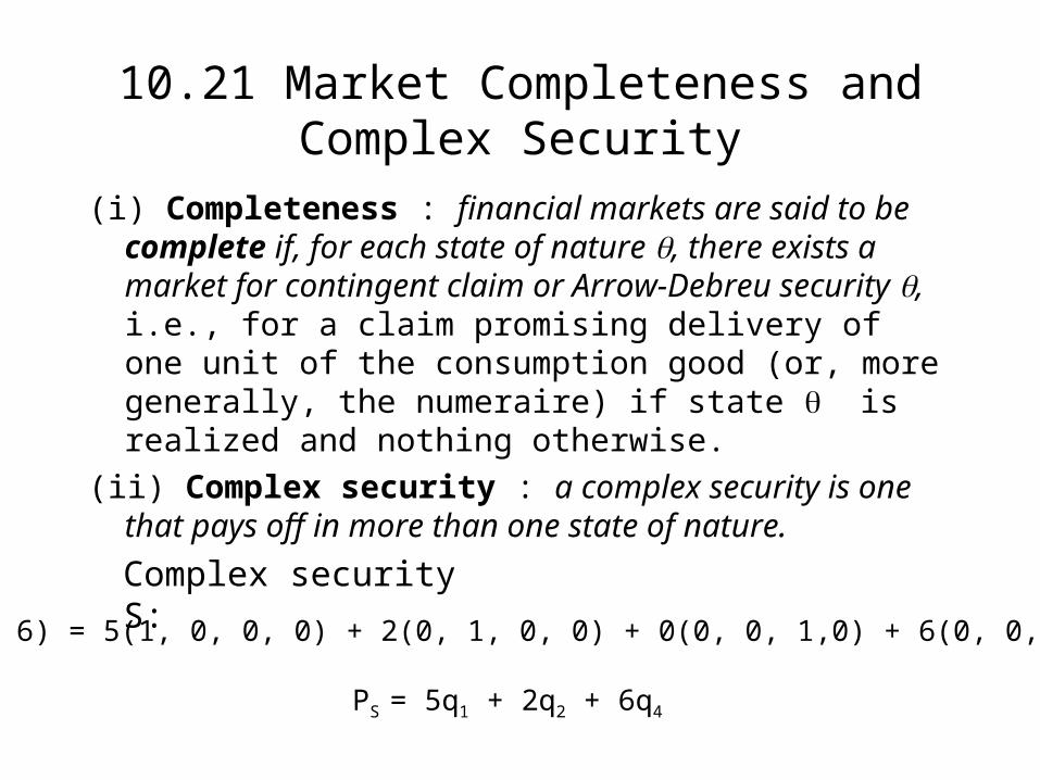
10.21 Market Completeness and Complex Security

(i) Completeness : financial markets are said to be complete if, for each state of nature , there exists a market for contingent claim or Arrow-Debreu security , i.e., for a claim promising delivery of one unit of the consumption good (or, more generally, the numeraire) if state is realized and nothing otherwise.

(ii) Complex security : a complex security is one that pays off in more than one state of nature.

(5, 2, 0, 6) = 5(1, 0, 0, 0) + 2(0, 1, 0, 0) + 0(0, 0, 1,0) + 6(0, 0, 0, 1)

PS = 5q1 + 2q2 + 6q4

Complex security S:

• Proposition 10.1. If markets are complete, any complex security or any cash flow stream can be replicated as a portfolio of Arrow-Debreu

securities. • Proposition 10.2. If M = N, and all the M complex

securities are linearly independent, then (i) it is possible to infer the prices of the A-D state-contingent claims from the complex securities' prices and (ii) markets are effectively complete.

Linearly independent = no complex security can be replicatedas a portfolio of some of the other complex securities.

(3, 2, 0) (1, 1, 1) (2, 0, 2)

(1, 0, 0) = w1(3, 2, 0) + w2(1, 1, 1) +w3(2, 0, 2)Thus, 1 = 3w1 + w2 + 2 w3

0 = 2 w1 + w2

0 = w2 + 2 w3

1 0 0

0 1 0

0 0 1

www

www

www

2 1 0

0 1 2

2 1 3

33

23

13

32

22

12

31

21

11

t=0123...T

-I0 1FC~

2FC~

3FC~...TFC~

T

1t

N

1,t,t0 CFqINPV (8.4)

10.3 Constructing State Contingent Claims Prices in a Risk-Free World: Deriving the

Term Structure

Table 10.2 Risk-Free Discount Bonds as Arrow-Debreu Securities

Current Bond Price Future Cash Flows

t=0 1 2 3 4 ... T -q1 $ 1000 -q2 $ 1000 ... -qT $ 1000

where the cash flow of a "j period discount bond" is just

t=0 1 ... j j+1 ... T -qj 0 0 $ 1000 0 0 0

• (i) 77/8% bond priced at 109 25/32, or $1'098.8125 / $ 1'000 face value

(ii) 55/8% bond priced at 100 9/32, or $1'002.8125 / $ 1'000 face value

• The coupons of these bonds are respectively,

.07875 * $ 1'000 = $ 78.75 / year

.05625 * $ 1'000 = $ 56.25 / year

Table 10-3 Present and Future Cash Flows for Two Coupon Bonds Bond Type Cash Flow at Time t t=0 (’00) 1 2 3 4 5 77/8 bond : -1097.8125 78.75 78.75 78.75 78.75 1078.75 55/8 bond : -1002.8125 56.25 56.25 56.25 56.25 1056.25

Table 10-4 Eliminating Intermediate Payments

Bond Cash Flow at Time t t=0 1 2 3 4 5 -1x 77/8 bond : +1097.8125 -78.75 -78.75 -78.75 -78.75 -1078.75 +1.4x 55/8 bond : -1403.9375 78.75 78.75 78.75 78.75 1478.75 Difference : -306.125 0 0 0 0 400.00

Price of $1.00 in 5 years = $ 0.765

Recovering the term structure:

• Suppose we observe risk-free bonds with 1,2, 3 and 4 year maturities, all selling at par, with coupons of 6%, 6.5%, 8.2% and 9.5% respectively

• Term structure is constructed as per:• r1 = 6%• r2 solves yielding r2 =

6.5113%• Similarly r3 = 8.2644% and r4 = 9.935%

221 )r1(

1065

r1

651000

Table 10-5 Date Claim vs. Discount Bond Price

Price of a N year claim Analogous Discount Bond Price ($ 1,000 denomination)

N = 1 q1 = 1/1.06 = .94339 $ 943.39 N = 2 q2 = 1/(1.065113)2 = .88147 $ 881.47 N = 3 q3 = 1/(1.072644)3 = .81027 $ 810.27 N = 4 q4 = 1/1.09935)4 = .68463 $ 684.63

Table 10-6 Discount Bonds as Arrow-Debreu Claims

Bond Price (t=0) CF pattern t=1 2 3 4 1 yr. discount -943.39 $ 1000 2 yr. discount -881.47 $ 1000 3 yr. discount -810.27 $ 1000 4 yr. discount -684.63 $ 1000

Table 10-7 Replicating the Discount Cash Flow

Bond Price (t=0) CF pattern t=1 2 3 4 .08-1 yr. discount (.08)(-943.39) = -75.47 $ 80 (80 state 1 A-D claims) .08-2 yr. discount (.08)(-881.47) = -70.52 $ 80 (80 state 2 A-D claims) .08-3 yr. discount (.08)(-810.27) = -64.82 $ 80 … 1.08-4 yr.discount (1.08)(-684.63) = -739.40 $1080

P(4yr.8%)=$950.21

Replicating 80 80 80 1080

...2 at t $1

0=at t .881472 at t 25$

1 at t $1

0=at t .943391at t 60$p

...

r1

00.125$

r1

00.160$ 2

21

...)065113.1(

00.1)25($

06.1

00.1)60($

2

etc. ... r1

150

r1

25

r1

603

32

21

Evaluating a risk-free project as a portfolio of A-D securities= discounting at the term structure.

Evaluating a CF: 60 25 150 300

Appendix 10.1. Forward Prices and Forward Rates

22111 )r1()f1)(r1(

33

2211 )r1()f1)(r1(

3312

22 )r1()f1()r1( , etc.

Table 10-11 Creating a $1000 Payoff

t = 0 1 2 Buy .939 x 2-yr bonds - 939 61.0 1000 Sell short .939 x 1-yr bonds + 939 -995.34 0 -934.34 1000

Table 10-10 Locking in a Forward Rate

t = 0 1 2 Buy a 2-yr bond - 1000 65 1065 Sell short a 1-yr bond + 1000 -1060 0 - 995 1065

10.4 The Value Additivity Theorem

bac z~Bz~Az~ , for some constant coefficients A and B. (10.2)

pc = Apa + Bpb.

s

sisi b,ai zqp (10.3)

s

basbssass

sbsass

scsc BpApzBqzAqBzAzqzqp

Diversifiable risk is not priced

• Suppose a and b are negatively correlated

• c is less risky, yet pc must be « in line » with pa and pb

• Suppose a and b are perfectly negatively correlated. Can be combined to form d, risk free

• pd must be such that holding d earns the riskless rate

• How can the risk of a and b be remunerated?

Ch.8 Options and Market Completeness

• 8.1 Introduction• 8.2 Using Options to Complete the Market: An

Abstract Setting• 8.3 Synthesizing State-Contingent Claim: A First

Approximation• 8.4 Recovering Arrow-Debreu Prices from Option

Prices: A Generalization• 8.5 Arrow-Debreu Pricing in a Multiperiod Setting• 8.6 Conclusions

10.5 Using Options to Complete the Market: An Abstract Setting

• Proposition 10.3. A necessary as well as sufficient condition for the creation of a complete set of A-D securities is that there exists a single portfolio with the property that options can be written on it and such that its payoff pattern distinguishes among all states of nature.

• Proposition 10.4: If it is possible to create, using options, a complete set of traded securities, simple put and call options written on the underlying assets are sufficient to

accomplish this goal.

10.6 Synthesizing State-Contingent Claim: A First Approximation

• It is assumed that ST discriminates across all states of nature so that Proposition 8.1 applies; without loss of generality, we may assume that ST takes the following set of values:

where S is the price of this complex security if state is realized at date T. Assume also that call options are written on this asset with all possible exercise prices, and that these options are traded. Let us also assume that for every state .

N21 S...S...SS

1SS

• Consider, for any state , the following portfolio P:• Buy one call with E = • Sell two calls with E = • Buy one call with E = .

At any point in time, the value of this portfolio, VP, is

1ˆS

S

1ˆS

1ˆˆ1ˆP SE,SCSE,SC2-SE,SCV

ˆT

ˆT

ˆT

SSif0

SSif

SSif0

P to Payoff

ˆ1ˆ1ˆ1

ˆ SE,SC2SE,SCSE,SCq

E S, ) 1

E S, ) 1

2

S S 1

S 1

TS

Payoff

STC (T S

TC (T

E S, )STC (T

Figure 10-1 Payoff Diagram for All Options in the Portfolio P

10.7 Recovering Arrow-Debreu Prices from Option Prices: A Generalization

(i) Suppose that ST, the price of the underlying portfolio (we may think of it as a proxy for M), assumes a "continuum" of possible values.

(ii) Let us construct the following portfolio : for some small positive number >0, buy one call with

sell one call with

sell one call with

buy one call with .

2TSE

2TSE

2TSE

2TSE

E S T, ) 2 E S T, ) 2

E S T, ^ ) 2

E S T, ^ ) + 2

2S T^ 2S T

^ S T^ + 2S T

^ + + 2S T^

^ ^

Payoff

TS

S TC (T S TC (T

S TC (TS TC (T

Figure 10-2 Payoff Diagram: Portfolio of Options

A Generalization

(iii)Let us thus consider buying 1/ units of the portfolio. The total payment, when , is , for any choice of . We want to let , so as to eliminate the payments in the ranges

and ,

.The value of 1/ units of this portfolio is :

T T T2 2ˆ ˆS S S

11

0

T T Tˆ ˆS (S ,S )

2 2

T T Tˆ ˆS (S ,S )

2 2

T T T2 2 2 2

1 ˆ ˆ ˆ ˆC S,E S C S,E S C S,E S C S,E ST

2T2T2T2T1

0SE,SCSE,SCSE,SCSE,SC lim

2T2T

0

2T2T

0

SE,SCSE,SClim

SE,SCSE,SClim

0 0

2T22T2 SE,SCSE,SC

The value today of this cash flow is :

.

S,SS if 50000

S,SS if 0CF

2T2TT

2T2TT ~

T

2T22T2 SE,SCSE,SC50000

1T2

2T2

2T

1T SE,SCSE,SCS,Sq (10.4)

(iv)

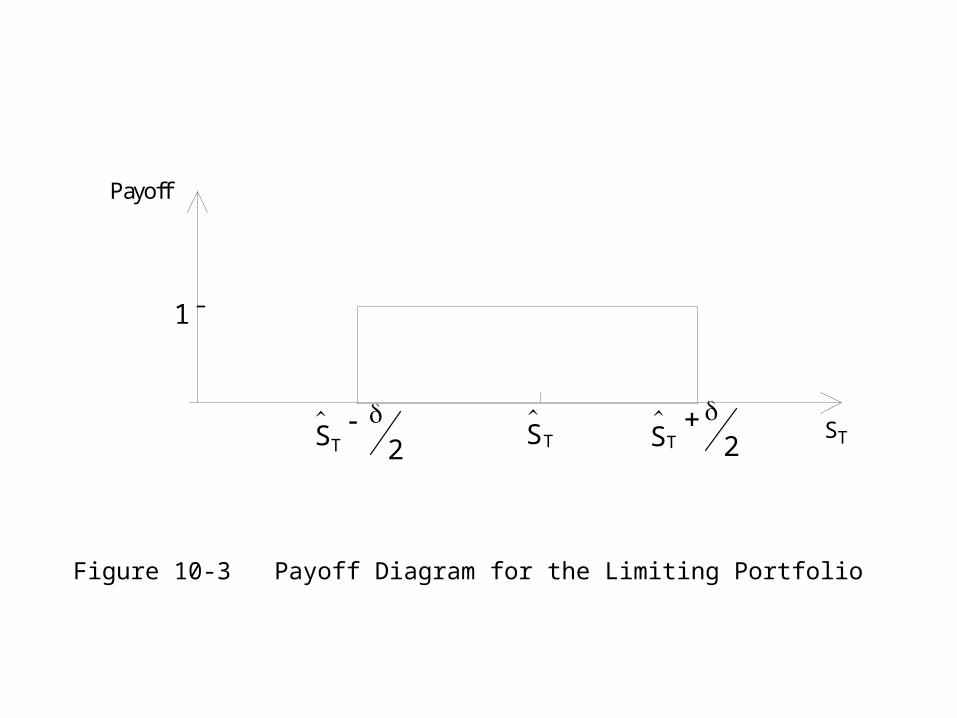
ST

2ST

2

ST

1

Payoff

TS

Figure 10-3 Payoff Diagram for the Limiting Portfolio

Table 10.8 Pricing an Arrow-Debreu State Claim

Payoff if ST = E C(S,E) Cost of position 7 8 9 10 11 12 13 C (C)= q

7 3.354

-0.895

8 2.459 0.106

-0.789 9 1.670 +1.670 0 0 0 1 2 3 4 0.164 -0.625

10 1.045 -2.090 0 0 0 0 -2 -4 -6 0.184 -0.441

11 0.604 +0.604 0 0 0 0 0 1 2 0.162 -0.279

12 0.325 0.118 -0.161

13 0.164 0.184 0 0 0 1 0 0 0