Radner Equilibrium: Definition and Equivalencewith Arrow-Debreu Equilibrium

Econ 2100 Fall 2017

Lecture 24, November 28

Outline

1 Sequential Trade and Arrow Securities2 Radner Equilibrium3 Equivalence between Arrow-Debreu and Radner Equilibria4 Assets and Asset Markets

Timing of Trades in Arrow-Debreu

RemarkIn an Arrow-Debreu economy, all decisions are made at date 0.

Individuals exchange promises to deliver and receive quantities of the goodsaccording to the state that is realized.

Tomorrow, one of the states occurs, and these promises are carried throughexactly as planned, without changes.

What if tomorrow, after the state is known, there were also markets for the Lgoods?

Is there an incentive to trade in these spot markets?

Spot Markets Do Not Matter in Arrow-Debreu

FactGiven an Arrow-Debreu equilibrium, there are no incentives to trade in spotmarkets.

Proof.Suppose not: consumers can find a mutually beneficial trade in some state t.

Thus, there exist a feasible allocation that all consumers pefer weakly to theequilibrium bundle, with at least one consumer preference being strict.

consumers trade only if they do better.

This new allocation is feasible, and Pareto dominates the Arrow-Debreuequilibrium.

But this is impossible, because the First Welfare Theorem holds.

This conclusion is disappointing as most real world markets are spot markets,not the forward markets imagined by an Arrow-Debreu economy.

Spot and Forward Markets

RemarkMost real world markets are spot, not forward.

ObjectiveReconcile this observation with a general equilibrium model with uncertainty similarto Arrow-Debreu.

IdeaSince the main role of state contingent commodities is to allow welfaretransfers across states...

... one can have similar transfers with just a few state-contingent markets.

This is because not all state-contingent commodities markets are neededprovided there is another way to transfer wealth across states.

Radner EquilibriumKen Arrow proposed the following model.

Individuals make decisions today and tomorrowonly one good is traded both today and tomorrow (and therefore used totransfer wealth across states), whileall other commodities are traded only tomorrow (these markets open afteruncertainty is resolved).

Today’s decisions depend on forecasts about tomorrow: trade is sequential, soexpectations are crucial.This equilibrium concept is called Radner equilibrium.

Main IdeaReplace forward markets with expectations about future spot markets.Given these expectations, consumers make decisions about welfare transfers acrossstates at date 0.When date 1 arrives, consumers trade in markets for physical goods.

Main Result: Radner and Arrow-Debreu Are EquivalentIf expectations are correct, and individuals have some effective way to transferwealth across states, a Radner equilibrium is equivalent to an Arrow-Debreuequilibrium.

Sequential Trading and Arrow SecuritiesDate 0Only one physical good becomes a state-contingent commodity: money.Amounts of money are traded for delivery if and only if a particular state occurs.

These are called Arrow securities (they are financial assets).

Date 1After some state occurs, there are spot markets where physical goods trade at spotprices (these prices can differ across states).

Individuals decide how much to trade of each good depending on (i) the spotprices, and (ii) how much they have traded in the state-contingent commoditythat corresponds to the realized state.

Expectations Are CrucialDate 0 trades reflect what consumers think will happen in the spot markets.

To decide how much to trade of the state-contingent commodity individualsmake consumption plans for each possible state; these plans depend on theirforecasts of the future spot prices.

Sequential Trading and Arrow SecuritiesConsider an exchange economy with Xi = RLS+ .

Notation

zi = (z1i , .., zSi ) ∈ RS denotes i’s trades in the state-contingent commodity;these contracts specify amounts to be delivered, or received, of commodity 1 ineach of the s states.

note: these date zero trades can be negative or positive.

q = (q1, .., qS ) ∈ RS denotes the prices of the Arrow securities.xi = (xi1, .., xiS ) ∈ RLS denotes i’s consumption plans vector;

xsi = (x1si , .., xLsi ) ∈ RL denotes i’s expected consumption in state s ;x1i = (x11i , .., x1Si ) ∈ RS represents expected trade in commodity 1, the onlycommodity for which there are also date 0 markets.

p = (p1, .., pS ) ∈ RLS is the vector of expected prices;ps ∈ RL is the expected price vector for the L goods in state s .

Expected prices and expected consumption plans are elements of RLS .

Note: that many items are “expected”, they represent planned choices.The consumer makes and plans choices given current and expected prices.There is no date 0 consumption (for simplicity).

OptimizationGiven current prices (q) and expected prices (p), each individual maximizes utility.

A plan includes current trades in the state-contingent commodity (zi ) andexpected spot market purchases (xi ).

Consumers’Choices at time 0At date 0, consumer i solves the following maximization problem

maxzi∈RS ,x∈RLS+

U (xi )

subject to

q · zi ≤ 0︸ ︷︷ ︸budget constraint at time 0

and ps · xsi ≤ ps · ωsi + p1szsi for each s︸ ︷︷ ︸expected budget constraints at time 1

There will be S budget constraints at date 1.These constraints are “in expectation” (from the point of view of date 0): xsiis expected consumption; ps are expected prices.Note that date 1 trading of good 1 has three components:

buy the desired amount for consumption,sell the endowment, andsell the realized state-contingent outcome of date 0 trades.

Date 0 Budget Constraint

Date 0The budget constraint at date 0 is

S∑s=1

qszsi ≤ 0

The individual must engage in zero net trades of the state-contingentcommodity.

Since the price vector is non-negative, if she promises to buy good 1 in state s(zsi > 0), she must also promise to sell it in some other state t (zti < 0).

This is because she has no income at date 0 and she cannot promise to spendmore than she makes

one could add a positive date 0 endowment (and consumption), withoutaffecting this logic.

The date 0 budget constraint is homogeneous of degree zero in prices.

Therefore, we can normalize date zero prices (sum up to one).

Date 1 Budget ConstraintsDate 1The budget constraints at time 1 are

L∑l=1

plsxlsi ≤L∑l=1

plsωlsi + p1szsi for each s = 1, ...,S

At date 1, consumer i trades in the spot markets corresponding to the realizedstate; her wealth reflects the outcome of previous trades.

The budget constraint is homogeneous of degree zero in spot prices.

Here, we normalize by assuming that ps1 = 1 for each s .

Thus, an Arrow security promises to deliver one unit of money (good 1).

Since there are no restrictions on z , we may have zt < −ω1ti for some t:i sells money ‘short’(she promises to deliver more than she will have); if so, shemust buy some money on the spot market.

the ability to sell short is limited: consumption cannot be negative.

Arrow securities allow wealth transfers across states: at date 0, a consumercan buy a state s dollar and pay for it with a state t dollar.

If state s occurs, she uses the extra dollar to buy other goods;if state t occurs, she has one less dollar to buy other goods.

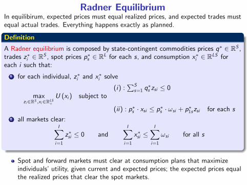
Radner EquilibriumIn equilibirum, expected prices must equal realized prices, and expected trades mustequal actual trades. Everything happens exactly as planned.

Definition

A Radner equilibrium is composed by state-contingent commodities prices q∗ ∈ RS ,trades z∗i ∈ RS , spot prices p∗s ∈ RL for each s, and consumption x∗i ∈ RLS foreach i such that:

1 for each individual, z∗i and x∗i solve

(i) :∑S

s=1 q∗s zsi ≤ 0

maxzi∈RS ,xi∈RLS+

U (xi ) subject to

(ii) : p∗s · xsi ≤ p∗s · ωsi + p∗1szsi for each s2 all markets clear:

I∑i=1

z∗si ≤ 0 andI∑i=1

x∗si ≤I∑i=1

ωsi for all s

Spot and forward markets must clear at consumption plans that maximizeindividuals’utility, given current and expected prices; the expected prices equalthe realized prices that clear the spot markets.

Radner and Arrow-Debreu Are EquivalentUnder the “rational expectations hypothesis” implicit in Radner equilibirum,planned behavior equals actual behavior and the timing of decisions isunimportant.

Proposition (Equivalence of Arrow-Debreu and Radner equilibria)

1 Suppose the allocation x∗ ∈ RLSI and the prices p∗ ∈ RLS++ constitute anArrow-Debreu equilibrium. Then, there are prices q∗ ∈ RS++ and tradesz∗ = (z∗1 , .., z

∗I ) ∈ RSI for the state-contingent commodity such that: z∗, q∗,

x∗, and spot prices p∗s for each s form a Radner equilibrium.2 Suppose consumption plans x∗ ∈ RLSI and z∗ ∈ RSI and prices q∗ ∈ RS++ andp∗ ∈ RLS++ constitute a Radner equilibrium. Then, there are S strictly positivenumbers µ1, .., µS such that the allocation x

∗ and the state-contingentcommodities price vector (µ1p

∗1 , .., µSp

∗S ) ∈ RLS++ form an Arrow-Debreu

equilibrium.

1 An Arrow-Debreu equilibrium becomes a Radner equilibrium if oneappropriately chooses trades and prices of the state contingent commodity.

2 A Radner equilibrium becomes an Arrow Debreu equilibrium if oneappropriately modifies spot prices to make them state-contingent prices.

The proof only needs to show that the two budget sets are the same.

From Arrow-Debreu to Radner

First, choose p1s = qs for each s (we can do this because...).

Write the Arrow-Debreu budget set as

BADi =

{xi ∈ RLS+ :

S∑s=1

ps · (xsi − ωsi ) ≤ 0}

Write the Radner budget set as

BRi =

xi ∈ RLS+ : there is zi ∈ RS s.t.

∑Ss=1 qszsi ≤ 0

and

ps · (xs − ωsi ) ≤ p1szsi for all s

We need to show these two sets are the same.

From Arrow-Debreu to Radner

Suppose x ∈ BADi ={xi ∈ RLS+ :

∑Ss=1 ps · (xsi − ωsi ) ≤ 0

}.

For each s letzsi =

1p1sps · (xs − ωsi ) .

ThenS∑s=1

qszsi =S∑s=1

p1szsi =S∑s=1

ps · (xs − ωsi ) ≤ 0

andps · (xs − ωsi ) = p1szsi for all s

Thus

x ∈ BRi =

xi ∈ RLS+ : ∃zi ∈ RS s.t.

∑Ss=1 qszsi ≤ 0and

ps · (xs − ωsi ) ≤ p1szsi for all s

.

From Arrow-Debreu to Radner

Let x ∈ BRi =

xi ∈ RLS+ : ∃zi ∈ RS s.t.

∑Ss=1 qszsi ≤ 0and

ps · (xs − ωsi ) ≤ p1szsi for all s

.Then, for some zi ∈ RS we have

S∑s=1

qszsi ≤ 0 and ps · (xs − ωsi ) ≤ p1szsi for all s

Summing over s yieldsS∑s=1

ps · (xs − ωsi ) ≤S∑s=1

p1szsi =S∑s=1

qszsi ≤ 0

Therefore x ∈ BADi ={xi ∈ RLS+ :

∑Ss=1 ps · (xsi − ωsi ) ≤ 0

}.

From Arrow-Debreu to Radner

We have shown that the budget set for Radner and Arrow-Debreu are the same.

An Arrow-Debreu equilibrium yields a Radner equilibriumIf x∗, p∗ is an Arrow-Debreu equilibrium, then

x∗, z∗, q∗ = (p∗11, ..., p∗1S ) , and z∗si =

1p∗1sp∗s · (x∗si − ωsi )

is a Radner equilibrium.

Why?

If the budget sets are the same, maximizing utility in BADi implies maximizingutility in BRi .The spot markets clear because the Arrow-Debreu markets clear.The state contingent markets clear since

I∑i=1

z∗si =I∑i=1

1p∗1sp∗s · (x∗si − ωsi ) =

1p∗1sp∗s ·

(I∑i=1

(x∗si − ωsi ))≤ 0

From Radner to Arrow-Debreu

Choose µs such that µsp1s = qs for each s. Next, show the budget sets arethe same.

Prove the rest as homework assignment.

Asset Markets in General EquilibriumNext, we model financial assets (rather than state contingent commodities), ina setup similar to Radner’s.A unit of an asset gives the holder the right to receive some payment in thefuture.

By convention, good 1 is the unit of accounts for assets.

DefinitionAn asset is a title to receive rs units of good 1 at date 1 if and only if state s occurs.

An asset is completely characterized by its return vectorr = (r1, .., rS ) ∈ RS

rs is the dividend paid to the holder of a unit of r if and only if state s occurs.

DefinitionThe return matrix R is an S × K matrix whose kth column is the return vector ofasset k . That is:

R =

r11 .. rk1 .. rK 1.. .. .. .. ..r1s .. rks .. rKs.. .. .. .. ..r1S .. rkS .. rKS

A row indicates the returns of all assets in one particular state.

Assets: Examples

ExampleAn asset that delivers one unit of good 1 in all states:

r = (1, .., 1)

If there is only one good, L = 1, this the risk-free (or safe) asset.

Why is this not safe with many goods?

Because the price of good 1 can change from state to state.

An asset matters insofar as it can be transformed into consumption goods; therate at which one can do this depends on relative prices.

ExampleAn asset that delivers one unit of good 1 in one state, and zero otherwise:

r = (0, .., 1, .., 0)

This is called an Arrow security.

Derivative Assets: ExampleAssets whose returns are defined in terms of other assets are called derivatives.These are very common in financial markets.

ExampleA European Call Option on asset r at strike price c gives its holder the right tobuy, after the state is revealed but before the returns on the asset are paid, oneunit of asset r at price c .

What is the return vector of this European call option?

The option will be exercised only if rs > c since in the opposite case one losesmoney (equality does not matter);

hencer (c) = (max {0, r1 − c} , ..,max {0, rS − c})

If r = (1, 2, 3, 4), then

r (1.5) = (0, 0.5, 1.5, 2.5)

r (2) = (0, 0, 1, 2)

r (3) = (0, 0, 0, 1)

Budget Constraints with Asset MarketsGiven an asset matrx R, one can define prices and holdings of each asset.

q = (q1, .., qK ) ∈ RK are the asset prices, where qk is the price of asset k.zi = (z1i , .., zKi ) ∈ RK are consumer i’s holdings of each asset.

This is called a portfolio: it shows how many units of each asset i owns.

Assets are traded at time 0, while returns are realized at time 1. At that time,agents decide how much to consume and they trade on spot markets.

As in Radner, i’s budget constraints areK∑k=1

qkzki ≤ 0︸ ︷︷ ︸time 0

and ps · xsi ≤ ps · ωsi +K∑k=1

p1szki rsk for each s︸ ︷︷ ︸time 1

Income at time 1 is given by the value of endowment plus the income oneobtains by selling the returns of the assets one owns.

As usual, one can normalize the spot price of good one to be 1.

Assets vs State-contingent Commodity in Radner

QuestionWhat is the difference between these budget constraints

K∑k=1

qkzki ≤ 0 and ps · xsi ≤ ps · ωsi +K∑k=1

p1szki rsk for each s

and the ones in a Radner equilibrium?

Here, the dividens of the assets are given; one focuses only on the portfoliochoice.

In Radner, the dividends are constructed by the consumers’choice of trades inthe state-contingent commodity.

Formally, in Radner one implicitly assumes S different assets, each withreturns rs = 1 in state s and zero otherwise.

If S = K , we can write Radner using the z and r above:

zRadners =S∑s=1

zs rs .