Embed Size (px)
Citation preview

1
Introduction
清大電機系林嘉文 [email protected]
03-5731152
Chapter 1
Signal & Signal Processing
• Signal: quantity that carries information
• Signal Processing is to study how to represent,
convert, interpret, and manipulate a signal and
the information contained in the signal
• DSP: signal processing in the digital domain
2011/2/23 Digital Signal Processing 2

2
Signals & Systems
Signals
“Something” that carries information
Speech, audio, image, video, biomedical signals,
radar signals, seismic signals, etc.
Systems
“Something” that can manipulate, change, record,
or transmit input signals
Examples: CD, VCD/DVD
2011/2/23 Digital Signal Processing 3
“Discrete-Time” Signals vs. “Digital”
Signals
Discrete-Time signal
A “sampled” version of a continuous signal
What is the minimum sampling frequency which is enough
to perfectly reconstruct the original continuous signal?
Nyquist rate (Shannon sampling theorem)
Digital Signal
“Sampling” + “Quantization” + “Coding”
Quantization: discrete-time continuous-valued signal ->
discrete-time discrete-valued signal
Coding: use a binary number of finite bits (e.g., 8 bits) to
represent a sampled value
2011/2/23 Digital Signal Processing 4
3
Examples of Typical Signals
Speech and music signals - Represent air
pressure as a function of time at a point in space
Waveform of the speech signal“ I like digital
signal processing” :
2011/2/23 Digital Signal Processing 5
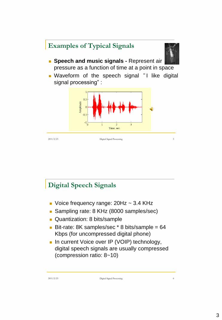
Digital Speech Signals
Voice frequency range: 20Hz ~ 3.4 KHz
Sampling rate: 8 KHz (8000 samples/sec)
Quantization: 8 bits/sample
Bit-rate: 8K samples/sec * 8 bits/sample = 64
Kbps (for uncompressed digital phone)
In current Voice over IP (VOIP) technology,
digital speech signals are usually compressed
(compression ratio: 8~10)
2011/2/23 Digital Signal Processing 6

4
Digital Audio Signals
Frequency range of human hearing system:
20Hz ~ 20 KHz
CD rate is 44,100 samples per second
16-bit samples
Stereo uses 2 channels
Number of bytes for 1 minute is
2 X (16/8) X 60 X 44100 = 10.584 Mbytes
What’s the length that a CD-ROM (680 Mbytes)
can store?
How about MP3?
2011/2/23 Digital Signal Processing 7
Examples of Typical Signals
Dow Jones Industrial Average
2011/2/23 Digital Signal Processing 8

5
Examples of Typical Signals
Electrocardiography (ECG) Signal - Represents
the electrical activity of heart
2011/2/23 Digital Signal Processing 9
ECG Signal
The ECG trace is a periodic waveform
One period of the waveform shown below
represents one cycle of the blood transfer process
from the heart to the arteries
2011/2/23 Digital Signal Processing 10

6
Examples of Typical Signals
Electroencephalogram (EEG) Signals -
Represent the electrical activity caused by the
random firings of billions of neurons in the brain
2011/2/23 Digital Signal Processing 11
Examples of Typical Signals
Seismic Signals - Caused by the movement
of rocks resulting from an earthquake, a volcanic
eruption, or an underground explosion
2011/2/23 Digital Signal Processing 12

7
Examples of Typical Signals
Black-and-white image - Represents light
intensity as a function of two spatial coordinates
I (x ,y)
2011/2/23 Digital Signal Processing 13
Examples of Typical Signals
Color Image – Consists of Red, Green, and
Blue (RGB) components
2011/2/23 Digital Signal Processing 14

8
Examples of Typical Signals
Surface Search Radar Image
2011/2/23 Digital Signal Processing 15
Digital Image
• An one mega-pixel image (1024x1024)
• Quantization: 24 bits/pixel for the RGB full-color
space
• File size of a color image: 1024x1024 pixels x
24 bits/pixel = 24 Mbits = 3 Mbytes (for
uncompressed digital image)
• How many uncompressed images can be
stored in a 2G SD flash-memory card?
• What is the compression ratio of JPEG used in
your digital camera?
2011/2/23 Digital Signal Processing 16

9
Digital Image (Cont.)
• In your image processing course, you were taught how
to do
– Edge detection (high-pass filtering)
– Image blurring or noise reduction (low-pass filtering)
– Object segmentation (spatial coherence classification)
– Image compression (retaining most significant info)
• The above are all about mathematical manipulations
– Could you give mathematical formulations for the
above manipulations?
– Could you characterize the frequency behaviors of
the above operations?
– Could you design an image processing tool to meet a
given spec?
2011/2/23 Digital Signal Processing 17
Example of Digital Image Processing
Blurring
Edge Detection Original Image
2011/2/23 Digital Signal Processing 18

10
2011/2/23 Digital Signal Processing 19
Examples of Typical Signals: Video
Video Camera
Video Cable
a single scan line
Voltage (proportional
to brightness)
Time
forehead
waveform of scan line shown
wall wall
active video sync and blanking
Video Monitor
hair hair
Examples of Typical Signals
Video signals - Consists of a sequence of
images, called frames, and is a function of 3
variables: 2 spatial coordinates and time
Frame 1 Frame 3 Frame 5
2011/2/23 Digital Signal Processing 20

11
Classifications of Signals (1/4)
Types of signal depend on the nature of the
independent variables and the value of the function
defining the signal
for example, the independent variables can be continuous or
discrete
likewise, the signal can be a continuous or discrete function of
the independent variables
for an 1-D signal, the independent variable is usually labeled as
time
A signal can be either a real-valued function or a
complex-valued function
A signal generated by a single source is called a scalar
signal, whereas a signal generated by multiple sources
is called a vector signal or a multichannel signal
2011/2/23 Digital Signal Processing 21
Classifications of Signals (2/4)
A continuous-time signal is defined at every instant of
time
A discrete-time signal is defined at discrete instants of
time, and hence, it is a sequence of numbers
A continuous-time signal with a continuous amplitude is
usually called an analog signal (e.g., speech)
A discrete-time signal with discrete-valued amplitudes
represented by a finite number of digits is referred to as
a digital signal
A discrete-time signal with continuous-valued amplitudes
is called a sampled-data signal
A continuous-time signal with discrete-value amplitudes
is usually called a quantized boxcar signal
2011/2/23 Digital Signal Processing 22

12
Classifications of Signals (3/4)
A signal that can be uniquely determined by a well-
defined process, such as a mathematical expression or
rule, or table look-up, is called a deterministic signal
A signal that is generated in a random fashion and
cannot be predicted ahead of time is called a random
signal
2011/2/23 Digital Signal Processing 23
Classification of Signals (4/4)
2011/2/23 Digital Signal Processing 24
quantized boxcar

13
Why DSP?
Mathematical abstractions lead to
generalization and discovery of new processing
techniques
Computer implementations are flexible
Applications provide a physical context
2011/2/23 Digital Signal Processing 25
Advantages of DSP (1/2)
Absence of drift in the filter characteristics
Processing characteristics are fixed, e.g. by binary
coefficients stored in memories
Independent of the external environment and of
parameters such as temperature and device aging
Improved quality level
Quality of processing limited only by economic
considerations
Desired quality level achieved by increasing the
number of bits in data/coefficient representation (SNR
improvement: 6 dB/bit)
2011/2/23 Digital Signal Processing 26

14
Advantages of DSP (2/2)
Reproducibility
Component tolerances do not affect system
performance with correct operation
No adjustments necessary during fabrication
No realignment needed over lifetime of equipment
Ease adjustment of processor characteristics
Easy to develop and implement adaptive filters,
programmable filters and complementary filters
Time-sharing of processor (multiplexing & modularity)
No loading effect
Realization of certain characteristics not possible or
difficult with analog implementations (e.g., linear phase)
2011/2/23 Digital Signal Processing 27
Limitations of DSP
Limited Frequency Range of Operation
Frequency range is technologically limited to values
corresponding to maximum computing capacities (e.g.,
A/D converter) that can be developed and exploited
Digital systems are active devices, thereby
consuming more power and being less reliable
Additional Complexity in the Processing of Analog
Signals
A/D and D/A converters must be introduced, thus adding
complexity to the overall system
Inaccuracy due to finite precision arithmetic
2011/2/23 Digital Signal Processing 28

15
Continuous-Time Sinusoidal Signals
2011/2/23 Digital Signal Processing 29
Properties:
For every fixed value of F, xa(t) is periodic (xa(t + Tp) = xa(t))
Continuous-time sinusoidal signals with distinct frequencies
are themselves distinct
Increasing the frequency F results in an increase in the rate
of oscillation of the signal
( ) cos
cos 2 ,
ax t A t
A Ft t
Representation of Sinusoidal Signals Using
Complex-Conjugate Exponentials
2011/2/23 Digital Signal Processing 30
( ) cos
2 2
a
j t j t
x t A t
A Ae e
cos sinje j
Euler identity:

16
Discrete-Time Sinusoidal Signals
2011/2/23 Digital Signal Processing 31
Properties:
A discrete-time sinusoid is periodic only if its frequency f is a
rational number
Discrete-time sinusoids whose frequencies are separated
by an integer multiple of 2 are identical
The highest rate of oscillation in a discrete-time sinusoid is
attained when = (or = )
( ) cos
cos 2
, 2 2
j n j n
x n A n
A fn
A Ae e n
Discrete-Time Sinusoidal Signals
2011/2/23 Digital Signal Processing 32

17
Harmonically Related Complex Exponentials
2011/2/23 Digital Signal Processing 33
0 02( ) , 0, 1, 2,...
jk t j kF t
ks t e e k
Continuous-time, harmonically related exponentials:
0( ) ( )jk t
a k k k
k k
x t c s t c e
For a continuous-time periodic signal with fundamental
period Tp = 1/F0, its Fourier series expansion is
1 1
2 /
0 0
N Nj kn N
k k k
k k
x n c s n c e
For a discrete-time periodic signal with fundamental period N,
its Fourier series expansion becomes
Analog-to-Digital (A/D) Conversion
2011/2/23 Digital Signal Processing 34

18
Sampling of Analog Signals (Cont.)
2011/2/23 Digital Signal Processing 35
Periodic/Uniform Sampling
Sampling rate (or sampling frequency) Fs = 1/T, where T
is the sampling period (interval)
( ), ax n x nT n
Sampling of Analog Signals (Cont.)
2011/2/23 Digital Signal Processing 36
Consider a sinusoidal signal
The discrete signal sampled at Fs can be represented as
( ) cos 2ax t A Ft
2
( ) cos 2 cosa
S
nFx nT A FnT A
F

19
Aliasing (1/2)
2011/2/23 Digital Signal Processing 37
The phenomenon of a continuous-time signal of higher
freq. acquiring the identity of a sinusoidal sequence of
lower freq. after sampling is called aliasing
An infinite number of continuous-time signals can lead to
the same sequence when sampled periodically
0
0
( ) cos 2
cos 2 / 2
cos 2
oa
S
S
F kFx nT A n
F
A nF F kn
A f n
0( ) cos 2 , where , 1, 2,..a k k Sx t A F t F F kF k
x n
Aliasing (2/2)
2011/2/23 Digital Signal Processing 38
Given the samples, draw a sinusoid through the values
cos(0.4 )x n n)4.2cos()4.0cos(
integer an is When
nn
n

20
Ambiguity in Sampling
2011/2/23 Digital Signal Processing 39
Sample the following three signals at 10 Hz
we obtain g1[n] = g2[n] = g3[n]
2011/2/23 Digital Signal Processing 40
Artifacts due to Sampling Aliasing (1/2)

21
2011/2/23 Digital Signal Processing 41
Artifacts due to Sampling Aliasing (2/2)
Sampling Theorem (1/2)
2011/2/23 Digital Signal Processing 42
Suppose any analog signal can be represented as a sum of sinusoids of different amplitudes
Thus if Fs 2Fmax= max(F1, F2, …, FN) then the
corresponding digital frequencies of the discrete-time signal
obtained by sampling the parent continuous-time sinusoidal
signal will be in the range −1/2 < fi < 1/2
No Aliasing
On the other hand, if Fs < 2Fmax, the normalized digital angular frequencies may foldover into a lower digital frequency ωi = ⟨2πFi/Fs⟩2π in the range −π < ω < π because of aliasing
1
( ) cos 2N
a i i i
i
x t A Ft

22
Sampling Theorem (2/2)
2011/2/23 Digital Signal Processing 43
Sampling Theorem
If the highest frequency contained in an analog signal xa(t) if
Fmax = B and the signal is sampled at a rate Fs > 2Fmax = 2B,
then xa(t) can be exactly recovered from its sample values
using the interpolation function
( )a a
n S S
n nx t x g t
F F
sin 2 / 2( )
2 2 / 2a a
n
B t n Bnx t x
B B t n B
If Fs = 2B
where / ( ) ( )a S ax n F x nT x n
sin 2( )
2
Btg t
Bt
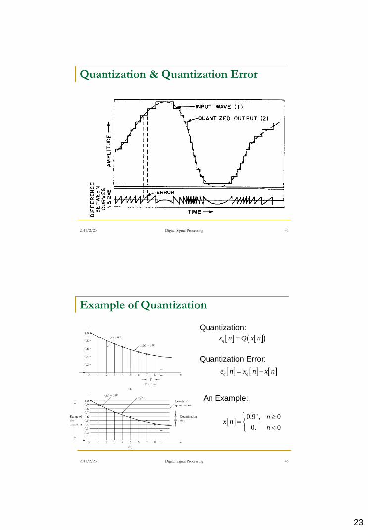
Quantization of Continuous-Amplitude
Signals
2011/2/23 Digital Signal Processing 44
Quantization: the process of converting a discrete-time
continuous-amplitude signal into a digital signal by
expressing each sample value as a finite number of digits
Quantization error/noise: the error introduced in
representing the continuous-valued signal by a finite set
of discrete value levels
non-invertible process
(many-to-one mapping)
23
Quantization & Quantization Error
2011/2/23 Digital Signal Processing 45
Example of Quantization
2011/2/23 Digital Signal Processing 46
qx n Q x n
q qe n x n x n
0.9 , 0
0. 0
n nx n
n
Quantization:
Quantization Error:
An Example:
24
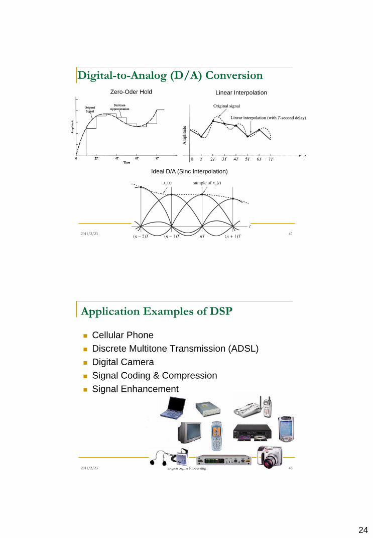
Digital-to-Analog (D/A) Conversion
2011/2/23 Digital Signal Processing 47
Zero-Oder Hold Linear Interpolation
Ideal D/A (Sinc Interpolation)
Application Examples of DSP
Cellular Phone
Discrete Multitone Transmission (ADSL)
Digital Camera
Signal Coding & Compression
Signal Enhancement
2011/2/23 Digital Signal Processing 48
25
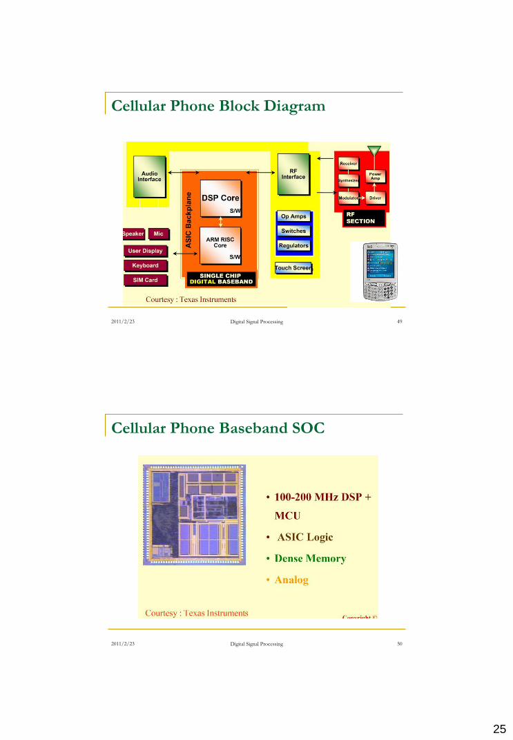
Cellular Phone Block Diagram
2011/2/23 Digital Signal Processing 49
Cellular Phone Baseband SOC
2011/2/23 Digital Signal Processing 50

26
Discrete MultiTone Modulation (DMT)
Core technology in the implementation of the
asymmetric digital subscriber line (ADSL) and very-
high-rate DSL (VDSL)
ADSL:
Downstream bit-rate: up to 9 Mb/s
Upstream bit-rate: up to 1 Mb/s
VDSL (e.g., CHT 光世代):
Downstream bit-rate: 13 to 26 Mb/s
Upstream bit-rate: 2 to 3 Mb/s
Distance: less than 1 km
Orthogonal Frequency-Division Multiplexing (OFDM)
for wireless communications (802.11 a/g/n, WiMAX,
LTE, DVB-T/H, etc.)
2011/2/23 Digital Signal Processing 51
ADSL modem
DMT
Transmitter
Receiver
2011/2/23 Digital Signal Processing 52

27
Digital Camera (1/5)
2011/2/23 Digital Signal Processing 53
Digital Camera (2/5)
CMOS Imaging Sensor
Increasingly being used in digital cameras
Single chip integration of sensor and other image
processing algorithms needed to generate final image
Can be manufactured at low cost
Less expensive cameras use single sensor with
individual pixels in the sensor covered with either a
red, a green, or a blue optical filter
2011/2/23 Digital Signal Processing 54

28
Digital Camera (3/5)
DSP-Based Image Processing Algorithms
Bad pixel detection and masking
Color interpolation
Color balancing
Contrast enhancement
False color detection and masking
Image and video compression
2011/2/23 Digital Signal Processing 55
Digital Camera (4/5)
Bad pixel detection and masking
2011/2/23 Digital Signal Processing 56

29
Digital Camera (5/5)
Color Interpolation and Balancing
2011/2/23 Digital Signal Processing 57
Signal Coding & Compression
Concerned with efficient digital representation of
audio or visual signal for storage and
transmission to provide maximum quality to the
listener or viewer
Speech coding: ITU-T G.711, G.723.1
Audio coding: MP3
Image coding: JPEG, JPEG-2000
Video Coding: MPEG-1 (VCD), MPEG-2 (DVD),
MPEG-4, H.264, Multi-View Coding (3-D TV)
2011/2/23 Digital Signal Processing 58

30
Signal Compression Example (1/4)
Original Speech
Data size: 330,780 bytes
• Compressed Speech (GSM 6.10)
Sampled at 22.050 kHz, Data size 16,896 bytes
Compressed speech (Lernout & Hauspie CELP 4.8kbit/s)
Sampled at 8 kHz, Data size 2,302 bytes
2011/2/23 Digital Signal Processing 59
Signal Compression Example (2/4)
Original Music
Audio Format: PCM 16.000 kHz, 16 Bits
(Data size 66206 bytes)
Compressed Music
Audio Format: GSM 6.10, 22.05 kHz
(Data size 9295 bytes)
Courtesy: Dr. A. Spanias
2011/2/23 Digital Signal Processing 60
31
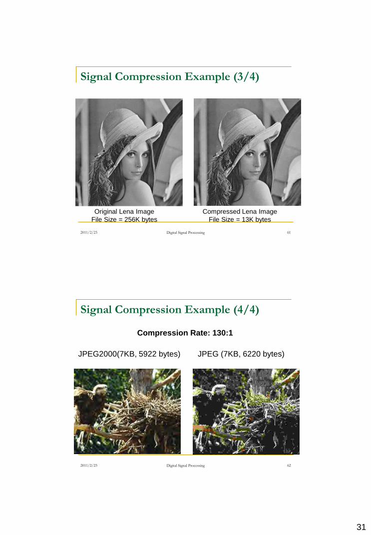
Signal Compression Example (3/4)
Original Lena Image
File Size = 256K bytes
Compressed Lena Image
File Size = 13K bytes
2011/2/23 Digital Signal Processing 61
Signal Compression Example (4/4)
2011/2/23 Digital Signal Processing 62
Compression Rate: 130:1
JPEG2000(7KB, 5922 bytes) JPEG (7KB, 6220 bytes)

32
Applications: Signal Enhancement
Purpose: To emphasize specific signal features
to provide maximum quality to the listener or
viewer
For speech signals, algorithms include removal
of background noise or interference
For image or video signals, algorithms include
contrast enhancement, sharpening and noise
removal
2011/2/23 Digital Signal Processing 63
Signal Enhancement Examples (1/4)
Noisy speech signal
(10% impulse noise)
Noise removed speech
2011/2/23 Digital Signal Processing 64

33
Signal Enhancement Examples (2/4)
2011/2/23 Digital Signal Processing 65
Signal Enhancement Examples (3/4)
Original image and its contrast enhanced version
Original Enhanced
2011/2/23 Digital Signal Processing 66

34
Signal Enhancement Examples (4/4)
Noisy image & denoised image
2011/2/23 Digital Signal Processing 67