Chapter 1 Ellipsometry: A Survey of Concept · 2018-08-15 · circular birefringence, and in case of a small absorption also circular dichroism. In this book the discussion is focused

Chapter 1Ellipsometry: A Survey of Concept

Christoph Cobet

Abstract Already the first attempts by Paul Drude in the late 19th century demon-strate the abilities of optical polarimetric methods to determine dielectric propertiesof thin layers. Meanwhile ellipsometry is a well-established method for thin filmanalysis. It provides material parameters like n and k even for arbitrary anisotropiclayers, film thicknesses in the range down to a few Ångström, and ellipsometry isused to analyze the shape of nm-scale surface structures. But, the determination ofsuch manifold information by means of light polarization changing upon reflectionat a sample surface requires appropriate optical models. This introductory chapterwill provide a general overview and explanation of theoretical and experimentalconcepts and their limitations. It will introduce the very basic data evaluation stepsin a comprehensive manner and will highlight the principal requirements for thecharacterization of functional organic surfaces and films.

1.1 Classification

Ellipsometry and other types of polarimetry are well known optical methods whichare used since more then 100 years for analytic purposes. Here, the term ellipsom-etry is certainly linked to the polarization sensitive optical investigation of planarsolid state structures (metals, semiconductors) with polarized light. Optical methodsin general benefit from the fact that they are usually non destructive and applicable invarious environments. The object under investigation can be stored in vacuum, gas,liquid, and even in solid ambiances as long as the surrounding material is transpar-ent within the spectral range of interest. By taking advantage of the polarizability oflight, it is possible to measure for example thin film properties like the refractive in-dex and the thickness with very high accuracy and without the need of a reference.Because of these abilities ellipsometry is meanwhile a very popular method usedin many different application fields. Accordingly, a couple of books, book chapters,

C. Cobet (B)Center for Surface- and Nanoanalytics, Johannes Kepler Universität Linz, Altenbergerstrasse 69,4040 Linz, Austriae-mail: [email protected]

K. Hinrichs, K.-J. Eichhorn (eds.), Ellipsometry of Functional Organic Surfaces andFilms, Springer Series in Surface Sciences 52, DOI 10.1007/978-3-642-40128-2_1,© Springer-Verlag Berlin Heidelberg 2014

1

mailto:[email protected]

http://dx.doi.org/10.1007/978-3-642-40128-2_1

2 C. Cobet

Fig. 1.1 Principle concept of ellipsometric and polarimetric techniques. The Polarization StateGenerator (PSG) and Polarization State Analyzer (PSA) may consist of a polarizer or a combina-tion of a polarizer and retardation component

and review articles provide already comprehensive information about the method el-lipsometry itself and the physical/mathematical background especially for thin filmapplications [1–7]. Therefore, it is not the intention to repeat here once again alltechnical details. We would rather like to provide in this chapter an overview aboutrelevant aspects which are needed to empathize the analytical possibilities concern-ing functional organic surfaces and films. Furthermore, we will address limitationsof the method and the underlying physical models.

The common concept behind the methods ellipsometry and polarimetry restsupon the analysis of a polarization change of light which is interacting with the ob-ject of interest. Here, we follow one of the definitions given by Azzam [8] in 1976which was discussed in connection to the 3rd International Conference on Ellipsom-etry. Accordingly “An ellipsometer (polarimeter) is any instrument in which a TE-EMW—transverse electric electromagnetic wave—generated by a suitable sourceis polarized in a known state, interacts with a sample under investigation, and theellipse (the state of polarization) of the radiation leaving the sample is analyzed”.This concept implies that both the polarization state of the light before and afterinteraction with the sample can be modified or determined (Fig. 1.1). Investigationsfor example of atmospheric and extraterrestrial phenomena where the polarizationproperties of the light source itself are analyzed or where the light polarization be-fore interacting with the object of interest is not accessible are not considered in thisdefinition [9]. Furthermore, only linear optical effects are considered and phenom-ena, where the light frequency is changed like in Raman scattering, second harmonicgeneration and sum frequency processes, are excluded.

With the definition above, ellipsometry can be used to analyze reflected, trans-mitted, scattered, and diffracted light (Fig. 1.2). Ellipsometric transmission mea-surements are so far preferentially used to analyze birefringence, optical activity,circular birefringence, and in case of a small absorption also circular dichroism. Inthis book the discussion is focused on the analysis of organic surfaces and strati-fied films in reflection type measurements. Thus, the sample is illuminated underan oblique angle of incidence and the specular reflection is analyzed (Fig. 1.2(a)).Accordingly, all presented theoretical models assume that the analysis takes placein the optical far field where the approximation of plane waves is reasonable i.e. thedistance between analyzer/detector and the sample has to be much larger than thewavelength and possible lateral inhomogeneities of the sample.

The applied optical models assume furthermore monochromatic or quasi-monochromatic electromagnetic waves which are reflected at the sample by re-taining total polarization of the incident light. The electromagnetic wave before and

1 Ellipsometry: A Survey of Concept 3

Fig. 1.2 Fundamentalinteraction of light whichincidents on different samplesunder an angle ϕi :(a) reflection,(b) transmission,(c) scattering, and(d) diffraction.All introduced ellipsometricproblems are reflectionmeasurements (red dashedbox)

after reflection is completely defined by an unique elliptical polarization state whichgives the method the name “ellipsometry”.

The term “polarimetry”, in contrast, is usually used in a more general contextincluding the analysis of non-specular reflected or scattered light from inhomoge-neous samples or surfaces (Fig. 1.2(b–d)). In this context polarimetry is often usedas a contact free method in order to determine morphology aspects [10]. Stronglyrelated to scattering processes is a partial depolarization of the light. As we willdiscuss later, this requires extended optical models. A strict delimitation betweenellipsometry and polarimetry, however, is neither possible nor helpful. In realityboth terms are used with much overlap and a number of specific approaches areused by related proper names (Sect. 1.5.6).

Bearing in mind that the fundamental electromagnetic theory remains the samefor all different regions of the spectrum, it is also not surprising that methods likepolarimetry and ellipsometry are applied in much the same way from the region ofradio frequencies over the infrared, visible and ultra violet to the X-/γ -ray spec-tral range. But due to experimental peculiarities, the knowledge transfer betweenthe communities is unfortunately low. This book will bridge in parts this spacingsby including all sections of the “optical” spectral range which includes here the in-frared, the visible, and the ultraviolet wavelength/frequency range. Nevertheless, itcould be particularly beneficial to consider also applications in the radio, radar, andmicrowave region. Related to the longer wavelength, the determination of structuraland morphological properties in this range is historically stronger in the focus. Re-spective theoretical models for the data processing are therefore rather sophisticatedand can be adapted for the optical spectral range [9, 11].

1.2 Historical Context

In a historical review the first observations of the polarization properties of light isdirectly linked to the discovery that light changes its polarization state after reflec-

4 C. Cobet

tion on, for example, glass windows of buildings and is associated with names likeEtienne-Louis Malus, David Brewster, and Augustin-Jean Fresnel. In the 1800’s thepolarization change of reflected light was used in a couple of works to study the op-tical properties of metals. A first description of elliptically polarized light attributesto Jamin [12–14]. He has observed this polarization after reflection of linearly po-larized light on metal surfaces which were decorated with transparent overlayers.It turned out, that the elliptical polarization is the most arbitrary polarization statewhose constituting parameters have to be determined when planar homogeneouslayers are investigated.1 For this reason, the name “ellipsometry” was established byRothen [15] almost 100 years later in 1945 for such kind of measurements. However,a first comprehensive description of the method as a technique to study the opticalproperties of thin films was given already by Paul Drude in the late 19th century. Hewas measuring the optical properties of metals under consideration of unintentionaland intentional overlayers. Furthermore, he could model the measured polarizationchanges by an extension/modification of Fresnel’s equation, which are originallymade for the reflection of light on a single planar interfaces, to the problem of twostacked interfaces [16–18]. With this approach it was possible to determine bulk andfilm dielectric properties as well as film thicknesses.

70 years later these analytical potentials attract a lot of attention in connectionwith the invention and development of semiconductor electronics. The investiga-tion of SiO2 films on Si is probably one of the best examples for the abilities ofthe method until now. On the other hand, the progress in semiconductor electronicsconsiderably accelerates the development of computers and the automation possi-bilities. With the help of microprocessors it was now possible to build automaticspectroscopic ellipsometers (SE) which made the method much more attractive fora wider community. Large steps forward in development and improvement are as-sociated to the work of Aspnes [19]. This progress also lead to more advanced ap-plications and setups with an appropriate spectral range and a reasonable resolution.In the following different angles of incidence or different polarization states of theincident light were used in order to extract more accurate information from rathercomplex samples. Meanwhile multi-layer structures, all kinds of optical anisotropy,magneto-optical effects, as well as 3D inhomogeneous structures are accessible.But the final breakthrough for the method is definitely linked to the availability ofeasy-to-use analysis software packages. Hence, it became possible to extract usefulinformation even for complicated sample structures with moderate efforts. In thiscontext it is also apparent why the optical characterization of organic films, whichare often anisotropic and inhomogeneous, was mostly restricted to reflection andtransmission measurements for a long time. The wide spread developments in therecent years are documented for example in the proceedings of the conference se-ries “International Conferences on Spectroscopic Ellipsometry” [20–24]. Concern-ing the newer developments we would also refer to a number of publications whichprovide further details [8, 25–29].

1Possible contributions of unpolarized light are ignored here.


Fig. 1.3 Basic data evaluation steps in an ellipsometric measurement. The left hand side of theflow chart depicts the determination of the polarizing properties of the sample which are repre-sented e.g. by the ellipsometric angles Ψ and � or in more general by polarization transformationcoefficients (PTC). In the right hand part these polarization parameters are translated in physicalsample parameters with the help of a qualitative sample model

1.3 Measurement Principles

1.3.1 Data Recording and Evaluation Steps

As it was mentioned, ellipsometry in principal determines polarization changesupon interaction with a sample. Subsequently it is possible to extract, for instance,layer thicknesses or dielectric properties in a “reference free” manner. Thus, twomajor data evaluation steps are needed in ellipsometry in order to receive informa-tion about the sample (Fig. 1.3). In parts they depend on each other. Neverthelessit is helpful to divide the problem in such basic steps and it seems worthwhile todiscuss these steps briefly to obtain a general understanding of the method.

All kinds of ellipsometers are primary measuring intensities with light sensitivedetectors. These intensities have to be related in the first evaluation step to the po-larization change induced by the sample (left hand part of Fig. 1.1). Therefore, eachellipsometer is recording the intensity with different incident light polarizations oranalyzer orientations in order to obtain relative intensities. With an appropriate setof such arrangements one can deduce out of it, how the sample under investigationchanges an arbitrary polarization of the incident light. It is evident that a respectivetheoretical formalism is needed which translates the detector signals to the polar-ization properties of the sample. As it will be discussed later, the probability of thesample to change the polarization of monochromatic light can be described for anisotropic sample, if no depolarization takes place, by two parameters. Quite oftenthe so-called ellipsometric angles Ψ and � are used. In case of anisotropic struc-tures up to 6 parameters are needed. According to reference [8] these parametersare denoted here as “polarization transformation coefficients” (PTC). If depolariza-tion effects are apparent, the number of parameters increases even further. For themoment it is important to note that the PTC’s depend on the angle of incidence, thewavelength, and probably on the sample orientation, too.

6 C. Cobet

Fig. 1.4 Principal of a rotating analyzer ellipsometer. The polarizer is here fixed with the transmis-sion axis tilted by 45◦ with respect to the plane of incidence. The intensity signal recorded at thedetector for a certain wavelength by rotating the analyzer is of a sinusoidal form with a periodicityof 2α

A very common and simple ellipsometer is the so-called rotating analyzer el-lipsometer. It’s principle arrangement and the signal recorded at the detector byrotating the analyzer is shown in Fig. 1.4 (q.v. Sect. 1.5). With at least three dif-ferent analyzer positions it is possible to assign the sinusoidal dependence of theintensity as a function of the rotation angle α by means of the two sin(2α) andcos(2α) Fourier-coefficients s2 and c2, respectively. With the later briefly explainedmathematical formalism it is possible to calculate Ψ and � of an isotropic non-depolarizing sample according to

tanΨ =√

1 + c2

1 − c2, cos� = s2√

1 − c22

. (1.1)

In a second step the information about the polarization change by the sample(the PTC’s or Ψ and �) should be translated in to intrinsic sample properties whichare not anymore related to a certain measurement configuration (right hand part inFig. 1.3). Such intrinsic sample properties are, for instance, layer dielectric func-tions, layer thicknesses, or volume fractions in inhomogeneous media.

In order to calculate intrinsic properties from the PTC’s again, an adequate the-oretical description is required. This means that the reflection process depicted inFig. 1.2(a) has to be specified in more detail. In the very simple and ideal case of aplanar abrupt surface of a infinitely thick isotropic sample this connection is givenby the well known Fresnel equation. The hereby defined reflection coefficients rpand rs for light polarizations parallel and perpendicular to the plane of incidencedetermine the ellipsometric angles Ψ and �:

rp

rs= tanΨ ei�. (1.2)

Light reflection from the backside of the sample is neglected in this model. Forstratified anisotropic media optical layer models are used in order to calculate therespective PTC’s for a given sample structure. In many cases, it is nevertheless pos-sible to define generalized Fresnel equations. The sample parameters are usually


obtained by a fit routine comparing the measured PTC’s with respective PTC’s cal-culated from the applied optical model.

At this point it is already obvious that the number of parameters which can bededuced is limited. By measuring Ψ and � in a single wavelength measurementat one angle of incidence and sample orientation, ellipsometry can provide two in-trinsic sample parameters. Therefore, it has to be ensured that there is a reasonablesensibility to the parameter of interest. In highly absorbing materials it can happenfor instance that the penetration depth of light is so small that the electric field in thelayer of interest is already damped too strongly. In anisotropic samples the specialcase might occur in which the electric field vector of the refracted light inside thesample is almost perpendicular to the optical axis of interest. In both examples thesensibility could be low. By using commercially available fit routines, such prob-lems can be tested by means of the so-called standard error. Finally, it has to beensured that the parameters of interest are not coupled to each other which happensif both of them change the polarization properties of the sample in the same manner.For example, it is sometimes difficult to measure a layer thickness and it’s refractiveindex independently from each other. In a numerical fit, the parameter coupling canbe tested by means of the covariance matrix of the standard errors.

The discussion of restrictions in the second evaluation step should emphasizethat qualitative information about the sample structure are essential in order to ob-tain good quantitative results. Indications for deficiencies in the assumed samplestructure are for example unexpected interference signatures or an inconsistent dis-persion of a deduced dielectric function.

The simple scheme of Fig. 1.3 does not include the important and sometimesdemanding step of the definition of appropriate measurement geometries (angle ofincidence, sample orientation, etc.) in order to achieve the best possible sensitivityto the sample parameters of interest. It is often not worthwhile to measure just inall possible configurations (e.g. in the whole accessible angle of incidence range).Configurations with low sensitivity to the parameter of interest (e.g. very high or lowangles of incidence) may just increase the error in the final result. Appropriate con-figuration can be chosen by some simple preliminary considerations. If necessary,these can be subsequently modified in an iterative procedure. Thin films are usuallybest measured at incidence angles near the Brewster angle of the respective substratematerial. In some cases it is more efficient to calculate the best configuration in apreliminary simulation.

Since all other evaluation steps are based on the chosen measurement configu-rations a final flow chart of an ellipsometric measurement may appear rather com-plicated (Fig. 1.5). In this resulting scheme the significance of an appropriate opti-cal model becomes again evident. It is important to remember that ellipsometry isinitially reference free measuring how a sample changes the polarization of an in-cident light beam. All subsequently derived parameters depend on the best possibleassumption of the sample structure and the validity of the applied optical models.Following Eugene A. Irene, who has brought this into phrase, this means in turnthat if the information about the sample structure is insufficient: “Ellipsometry isperhaps the most surface sensitive technique in the universe. However you oftendon’t know what it is you have measured so sensitively”.

8 C. Cobet

Fig. 1.5 Extended scheme of the data evaluation in an ellipsometric measurement. The two majorcalculation steps, which can be found already in the simplified representation of Fig. 1.3 are labeled1! and 2!

1.3.2 Determination of Ψ and �

The determination of Ψ and � or the more generalized PTC’s of a sample requiressome mathematical tools (calculation step 1© in Figs. 1.3 and 1.5). First of all asuitable description of polarized light is needed. Furthermore, all optical compo-nents including the sample under investigation have to be represented according totheir ability to change the state of polarization. These theoretical tools can be finallyused to calculate relative intensities which are measured at a detector or, in turn, todetermine the PTC’s of the sample from the measured intensities.

1.3.2.1 Polarized Light

To simplify the problem as much as possible, assumptions concerning the propaga-tion of light between optical components and the sample are necessary.

• Since linear optical effects are investigated each wavelength λ is addressed sepa-rately in a quasi-monochromatic approximation.

• The distances between the optical components are much larger than the wave-length and the coherence length of the light. We can assume planar transversalelectromagnetic (TEM) waves propagating only in forward direction from thelight source to the detector. In other words, all optical components interact inde-pendently, one after another, with the light and interferences between them areavoided. This assumption has to be critical reviewed, e.g. for laser light sourceswhere the coherence length is much larger than for conventional light sources andin near field experiments.


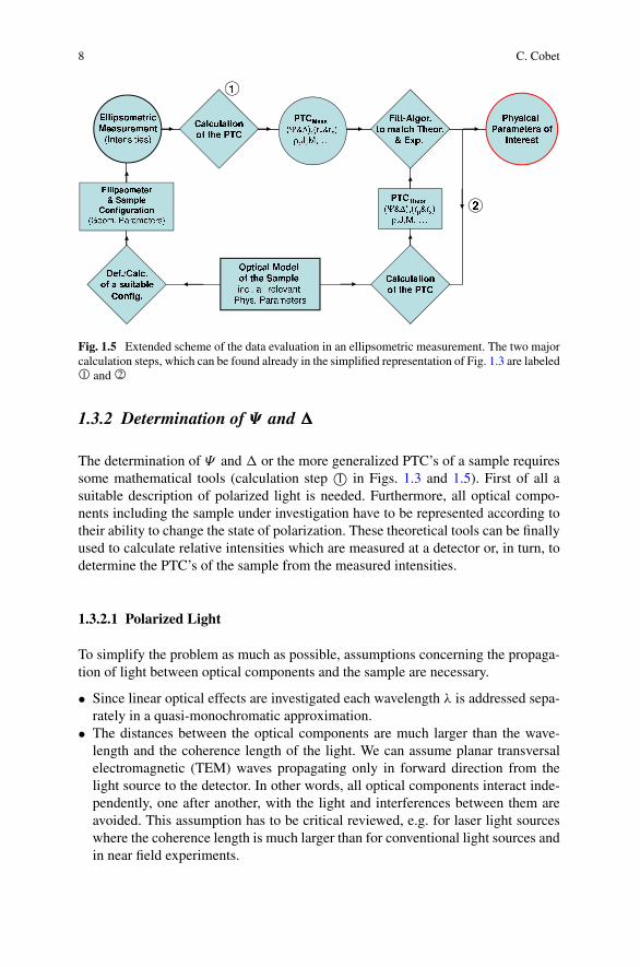
Fig. 1.6 Elliptically polarized light and the projected polarization ellipse. Mathematically the po-larization state is defined by three equivalent parameter sets [Ψ ′/�′—amplitude quotient and phasedifference], [ϑ /γ —azimuth angle and ellipticity], and χ = 1/ tanΨ exp[i�]

• The surrounding medium is assumed isotropic and homogeneous (air, vacuum,water, etc.). Thereby the polarization state does not depend on the propagationdirection and can be separately considered.

• The magnetic susceptibility is constantly one in all optical experiments and thepolarization of light is fully described by the electric fields.

For the mathematical description of a polarization one can choose without furtherloss of generality a Cartesian coordinate system so that the light propagates alongthe positive direction of the z-axis. A common description of an arbitrarily planarmonochromatic TEM wave is then given by

Ex = E0x exp[i(kz − ωt)

]exp[iδx],

Ey = E0y exp[i(kz − ωt)

]exp[iδy].

(1.3)

Equation (1.3) represents the general case of an elliptical polarization as illustratedin Fig. 1.6. The wave vector k = 2π/λ and the angular frequency ω = 2πν areconnected by the known dispersion relation for TEM waves in transparent media.The orientation of the two perpendicular basis vectors in x- and y-direction is freeof choice for the moment. The amplitudes E0x and E0y together with the phases δx

and δy for the x and y component, respectively, define the polarization of the light.This set of information can be merged in a so-called Jones vector [30]:

EJones =(

E0x exp[iδx]E0y exp[iδy]

). (1.4)

10 C. Cobet

However, the absolute phase is not measurable and the absolute intensity (I ∼E2

0x + E20y ) is an arbitrary value which is not of interest in an ellipsometric mea-

surement. The polarization state is therefore already fully defined by only two pa-rameters: The relative amplitude tanΨ ′ = E0x/E0y and phase �′ = δx − δy of the x

and y component. Sometimes these two parameters are combined in a single com-plex number χ = 1/ tanΨ ′ exp[i�′]. Another alternative representation refers to theellipse, which yields from a projection of the electric field vector to the x–y-plane.The respective parameter pair is given by the azimuth angle ϑ between the mainaxis of the ellipse and the x-axis and the ellipticity γ (Fig. 1.6). Please note thatthe parameters Ψ ′ and �′, which define here the polarization state of light, are ingeneral not identical with the previously defined Ψ and � values, which describehow the sample changes the polarization. Only in the special historically importantcase, where the incident light is chosen 45◦ linearly polarized with respect to theplane of incidence, both parameter sets match. Commercially available ellipsome-ters determine Ψ and � independent from the selected incident polarization.

So far, all representations of the polarization are only applicable for totally polar-ized light. Hence, they represent 100 % linear, circular or elliptically polarized lightand the constituting parameter pairs are of a well defined value. Unfortunately, thisis sometimes not sufficient and it is necessary to consider also partial polarizations.Possible sources of partial polarized light are

• non ideal polarizers,• lateral inhomogeneous samples (e.g. rough surfaces/interfaces or inhomogeneous

film thickness),• a divergent light beam (e.g. a short focal distance results in an uncertain angle of

incidence),• an insufficient spectral resolution and broad spectral line width, respectively.

Independent from the inbound polarization and the source of depolarization, par-tial polarization means that the well defined polarization is replaced by a statisticalmixture of different polarization states. In this view the components of the Jonesvector are now time dependent and polarization is measurable just as a time-average.A proper description of the partially polarized light requires therefore a third param-eter which for example characterizes the probability w to find a certain polarizationstate. Related to the fact that effective intensities (time-averaged fields) are finallymeasured, the three constituting parameters are often expressed in terms of intensi-ties. Complemented by the total intensity they form the 4 Stokes parameters [31]:

S0 = I,

S1 = Ix − Iy,

S2 = I+π/4 − I−π/4,

S3 = Il − Ir .

(1.5)

The first Stokes parameter contains simply the total intensity I of the light. Ix ,Iy , I+π/4, and I−π/4 are the intensities, which would pass through an ideal linear


polarizer oriented with the transmission axis in x, y, +π/4, and −π/4 direction, re-spectively. Il and Ir are the intensities, which would pass through ideal left and rightcircular polarizers. The total intensity resumes to I = Ix + Iy = I+π/4 + I−π/4 =Il + Ir . In case of totally polarized light S2

0 = S21 + S2

2 + S23 , while for partially or

unpolarized light S20 ≥ S2

1 + S22 + S2

3 . The degree of polarization is finally definedby:

P =√

S21 + S2

2 + S23

S20

= 2w − 1. (1.6)

For more comprehensive descriptions of the different representations of polar-ized light and the relation among these representations we would refer at this pointto respective literature about fundamental optics and ellipsometry [2, 4, 9, 32, 33].Because of similarities in operational concepts to quantum physics, the theory ofpolarized light is furthermore discussed in a number of rather theoretical publica-tions [11, 32, 34, 35]. An alternative description of partial polarized light by meansof coherency-matrices is described for example in references [2, 36].

1.3.2.2 Jones and Mueller Matrix Methods

The matrix methods of Jones [30] and Mueller [37–40] are by far the most popularmethods in order to describe the linear optical effects of polarizing optical elements.The Jones formalism is based on complex 2 × 2 matrices which are applied to theJones vector as defined in the previous section. The Mueller matrix formalism uses4 × 4 matrices with real elements which are applied to the Stokes parameters ar-ranged now in a column vector S = (S0, S1, S2, S3). The impact of a polarizingelement can thus be written as(

E′x

E′y

)= J

(Ex

Ey

)=

(Jxx Jxy

Jyx Jyy

)(Ex

Ey

),

⎛⎜⎜⎝

S′0

S′1

S′2

S′3

⎞⎟⎟⎠ = M

⎛⎜⎜⎝

S0S1S2S3

⎞⎟⎟⎠ =

⎛⎜⎜⎝

M00 M01 M02 M03M10 M11 M12 M13M20 M21 M22 M23M30 M31 M32 M33

⎞⎟⎟⎠

⎛⎜⎜⎝

S0S1S2S3

⎞⎟⎟⎠ .

(1.7)

The complex 2 × 2 Jones matrix contains 8 parameters including the absolutephase which is not measurable. If the absolute phase and additionally the absoluteintensity, which is also not if interest in ellipsometric measurements are ignored,the Jones matrix contains 6 relevant parameters that define the ability to changethe polarization. All optical components and any arbitrarily anisotropic samples canbe represented by means of these 6 parameters in a Jones matrix as long as nodepolarization takes place.

The 16 coefficients of the Mueller matrix contain information about intensitiespassing through polarizing elements. This includes information about the absolute

12 C. Cobet

intensity. Accordingly, the Mueller matrix contains 7 independent parameters, ifno depolarization takes place. In turn this means that 9 identities exist among the16 coefficients of a Mueller matrix in this case [39, 41]. It is thus feasible thatthe Mueller matrix of a non-depolarizing optical element can be calculated fromthe respective Jones matrix and vice versa except of the absolute phase [2, 42].However, in case of depolarization the 16 coefficients of a Mueller matrix becomeindependent and might include manifold orientation depending information about asample. But notice, the polarization state of the obtained partially depolarized lightis always fully characterized by only 3 parameters.

With the help of either the Jones or the Mueller matrix formalism it is now possi-ble to calculate the measurable intensities for different orientations of the polarizingelements in an ellipsometer. Therefore, the matrix representations of all optical el-ements including the sample under investigation are multiplied in the respectiveorder.

By a comparison of the measured intensities with those calculated, it is finallypossible to obtain the unknown sample polarization transformation coefficients(PTC). The latter can be represented for example either by the bare Mueller orJones matrix coefficients, the ellipsometric angles Ψ and �, or the (generalized)complex Fresnel coefficients. The choice of the most convenient representation de-pends on the sample under investigation and the specific ellipsometer type. Just likethe choice which parameters are used, the determination of PTC’s in practice alsodepends strongly on the sample properties and the ellipsometer type. If the intensityis for example continuously measured as a function of the rotation of a polarizingelement it is often beneficial to consider the Fourier transformation of the measuredsinusoidal signal. In case of an isotropic non-depolarizing sample, the two param-eters describing the polarization probability are then encoded in the sin(2α) andcos(2α) Fourier coefficients and can be determined thereafter algebraically by acomparison of coefficients. According to the sampling theorem, it is also sufficientto measure the sinusoidal signal with a minimum of three fixed positions in orderto obtain the two Fourier parameters in a fit algorithm. Finally, it is in some casesalso possible to measure at four specific positions [4] and to calculate the two PTC’sdirectly from the measured intensities.

1.3.3 Fresnel Coefficients

The second crucial step in an ellipsometric measurement now comprises the transla-tion of the obtained PTC’s to intrinsic sample properties like the dielectric functionor the layer thickness (calculation step 2© in Fig. 1.3). This problem of the light mat-ter interaction could be rather complicated in case of increasingly complex samplestructures. Therefore, only a few essential conclusions will be introduced which aretypically used for analyzing organic film structures.

It is reasonable to consider organic and anorganic materials as homogeneous ma-terials which are well characterized by its macroscopic optical properties i.e. the


macroscopic polarizability, dielectric function, or refractive index. This approxi-mation is adequate as long as the wavelength is much larger than the size of theconstituting molecules and larger than the unit cell of the crystal. It is often possi-ble to assume a stratified sample structure, which allows a description of the lightmatter interaction with planar TEM waves. With these two assumptions it is pos-sible to deduce complex reflection and transmission coefficients, which provide alink between the measured Ψ and � or PTC’s and the intrinsic sample parameters.The sample parameters are usually determined within a fit procedure. This part ofthe data evaluation is often called “optical modeling”. It is usually the most discrim-inating step in the data evaluation because it rests on a correctly assigned samplestructure which has to be critical reviewed in advance.

1.3.3.1 Dielectric Function

The optical properties of a homogeneous material can be encountered in the macro-scopic Maxwell equations i.e. the constitutive relations. These relations connect themacroscopic electric field E with the dielectric displacement D as well as the mag-netic induction B and magnetic field H according to the polarization and magneti-zation of the material. Again, three simplifications can be used:

• In the optical frequency range the macroscopic magnetization is always zero.• The discussed ellipsometric measurements comprise only linear optical effects

and higher order contributions can be neglected.• Spatial dispersion effects are negligible in homogeneous media.

As a result, the response of the material to an electric field is defined by the macro-scopic polarizability P .2 The material equations in a Fourier representation can bewritten as

D[ω] = ε0E[ω] + P[E[ω],ω]

= ε0ε[ω]E[ω],B[ω] = μ0H [ω].

(1.8)

In optical problems the magnetic field strength is connected with the magnetic in-duction density just by the free space permeability μ0. The macroscopic electricfield strength is connected to the displacement density by the free space permittivityε0 and the dielectric tensor ε which depends on angular frequency ω. In absorb-ing materials ε = ε1 + iε2 is a complex tensor and the imaginary part of the tensorcomponents is proportional to energy dissipation and thus to the absorption of thelight. In case of isotropic media the dielectric tensor reduces to a scalar dielectric

2P is the spatial average of the induced dipole moments per unit volume.

14 C. Cobet

Table 1.1 Equivalent quantities for the linear optical properties of homogeneous media

Real part Imaginary part

Dielectric function: ε ε1 = n2 − k2 ε2 = 2nk

Refractive index: n = √ε n =

√(ε1 +

√ε2

1 + ε22)/2 k =

√(−ε1 +

√ε2

1 + ε22)/2

Susceptibility: χ = ε − 1 χ1 = ε1 − 1 χ2 = ε2

Optical conductivity: σ σ1 = ωε0ε2 σ2 = −ωε0(ε1 − 1)

Loss function: −ε−1 −ε1

ε21 + ε2

2

ε2

ε21 + ε2

2

Phase velocity: vp = c/n1√

ε0μ0

1

n

1√ε0μ0

1

k

function.

ε =⎛⎝ε 0 0

0 ε 00 0 ε

⎞⎠ = ε

⎛⎝1 0 0

0 1 00 0 1

⎞⎠ (isotropic materials). (1.9)

As already seen in (1.8) a couple of equivalent quantities can be used in order todescribe the linear optical properties of a medium. Most widely used is the complexrefractive index n = n + ik where the real part n refers to the refractive index oftransparent media. The imaginary part k is the absorption coefficient of a medium.Other common representations of the optical response function and the relationsamong them are summarized in Table 1.1.

In case of an anisotropic sample with three intrinsic Cartesian optical axes thedielectric tensor can be diagonalized in the form

ε =⎛⎝εx 0 0

0 εy 00 0 εz

⎞⎠ (anisotropic materials). (1.10)

The dielectric tensor is defined now by three independent dielectric functions εx ,εy , and εz which determine the different polarizabilities for electric fields in the cor-responding directions. Such a matrix is suitable for biaxial crystals of e.g. triclinic,monoclinic, and orthorhombic symmetry. Uniaxial crystals of e.g. hexagonal, tetrag-onal, trigonal, and rhombohedral symmetry are defined analogue but only with twoindependent components [43]. As indicated before, in isotropic materials e.g. cubiccrystals, all components are equal. If the sample is placed in an arbitrary orientationin the ellipsometer, the matrix (1.10) has to be transposed by a rotation about theEuler angles.

Organic molecules like sugar, however, have often an intrinsic handedness/chirality. This yields an optical activity and circular dichroism if light is transmittedthrough a film or liquid solution. The dielectric tensor of such materials is now nolonger symmetric. But in case of vanishing absorption (optical activity) the tensor


is still Hermitian (εij = εij∗). The constitutive Maxwell relation is than written as

D[ω] = εaE[ω] + iε0G[ω] × E[ω], (1.11)

where εa is the dielectric tensor for vanishing optical activity. The vector G is point-ing in the direction of the light propagation and is called the gyration vector [44].

The optical rotation due to the Faraday effect which may emerge in the presentsof a magnetic field is defined analogously [43, 44]

D[ω] = εaE[ω] + iε0γB[ω] × E[ω]. (1.12)

1.3.3.2 Fresnel Equations

As mentioned before the link between sample properties like the dielectric functionand its polarization properties given either by Ψ and � or by the PTC’s can be ob-tained by the definition of reflection and transmission coefficients. These complexcoefficients determine to which amount the electric field amplitudes of the incidents- and p-polarization component are attributed to the respective fields in the re-flected and transmitted beam and determine the relative phase shifts among thesecomponents.

For a single interface between two isotropic homogeneous media these relationscan be obtained as a result of the boundary conditions committed by the Maxwellequations. They are known as the Fresnel equations of the form

rp = n2 cosϕi − n1 cosϕt

n2 cosϕi + n1 cosϕt

,

rs = n1 cosϕi − n2 cosϕt


,

tp = 2n1 cosϕi


,

ts = 2n1 cosϕi


.

(1.13)

n1 and n2 are the complex refractive indices of the incident and refractive media,respectively, and the angles of incidence ϕi and refraction ϕt are described by Snell’slaw (n1 sinϕi = n2 sinϕt ).

The assumption of a sample, which consists of only a single perfectly smoothsurface, is unfortunately very unrealistic. In practice at least unintentional surfaceoverlayers or a finite surface roughness are not negligible. Nevertheless, the Fresnelequations are often used as a good approximation. The obtained dielectric functionis then the so-called pseudo dielectric function [6].

〈ε〉 = sin2 φ

(1 + tan2 φ

(1 − ρ

1 + ρ

)2), ρ = rp

rs= tanΨ ei�. (1.14)

16 C. Cobet

1.3.3.3 Homogeneous Stratified Media

A simple optical layer model of practical importance describes a single isotropiclayer (l) of the complex refractive index nl and thickness d on a substrate (s) withthe complex refractive index ns . Light, which incidences from the ambient (a) withthe refractive index na , is reflected on the surface and the interface between layerand substrate. Due to multiple reflections within the layer, the overall reflected elec-tric fields parallel and perpendicular to the plane of incidence add up by a geomet-ric series. The summations gives the Airy formula for the so-called 3-phase model[2, 17, 44–46]:

rp = ralp + rlsp ei2β

1 + ralp rlsp ei2β,

rs = rals + rlss ei2β

1 + rals rlss ei2β

,

(1.15)

where ralp/s and rlsp/s are the Fresnel reflection coefficients on the ambient layerboundary and the layer substrate boundary, respectively (1.13). The phase factor β

is given by

β = 2π

λd

√n2

l − n2a sin2 φa = 2π

λ(d nl) cosφl. (1.16)

λ is the wavelength of the light in vacuum and φa the angle of incidence. It will beshown later that generalized complex “Fresnel” coefficients as defined in Eq. (1.15)can be obtained also for complex anisotropic structures. Before it should be men-tioned that the reflection coefficients of the 3-phase model contain already 5 pa-rameters which determine the optical properties of the sample. Even if the substratedielectric function is known, we have already one parameter more than a singlemeasurement at a given angle of incidence can deliver. An examination of the phasefactor β furthermore illustrates the coupling of nl and d . An unambiguous determi-nation of the thickness and the optical properties is possible by means of multipleangle of incidence measurements. A solution for very thin layers with d � 1 nmwill be discussed in Chap. 10.

The problem of a multilayer structure with planar parallel interfaces can besolved with the help of a 2 × 2 transfer matrix methods [2, 44, 47–51]. To someextend similar to the Jones matrix formalism, it is possible to connect the electricfields of the forward and backward traveling waves at each interface by a transfermatrix which is defined by the Fresnel coefficients for this specific interface and thusdepends on the refractive index on both sides as well as the incident angle. In con-trast to the Jones matrix formalism the distance between the interfaces is assumednow to be smaller than the coherence length of the light and interference betweenthe forward and backward traveling waves becomes possible. Consequently, a prop-agation matrix has to be introduced, which implements a (complex) phase factor tothe electric fields crossing a given layer. The reflection and transmission coefficients(rp/rs and tp/ts ) of the whole slab are finally obtained by the product of all transferand propagation matrices in the respective order.


Table 1.2 Reflection coefficients for parallel and perpendicular polarized light reflected at thesurface of an uniaxial anisotropic material if the optical axis c coincides with one of the threehigh symmetry orientations [2, 52]. (c ‖ x)—c parallel to the plane of incidence and the surface;(c ‖ y)—c perpendicular to the plane of incidence and parallel to the surface; (c ‖ z)—c perpen-dicular to the surface and parallel to the plane of incidence. ε⊥ and ε‖ correspond to the dielectrictensor components perpendicular and parallel to the optical axis i.e. the ordinary and extraordinarydielectric function

p polarization (rpp) s polarization (rss )

(c ‖ x):

√ε⊥ε‖ cosφi −

√ε⊥ − sin2 φi

√ε⊥ε‖ cosφi +


cosφi +√

ε⊥ − sin2 φi

cosφi −√

ε⊥ − sin2 φi

(c ‖ y):ε⊥ cosφi −


ε⊥ cosφi +√

ε⊥ − sin2 φi

cosφi +√

ε‖ − sin2 φi

cosφi −√

ε‖ − sin2 φi

(c ‖ z):

√ε‖ε⊥ cosφi −

√ε‖ − sin2 φi

√ε‖ε⊥ cosφi +

√ε‖ − sin2 φi

cosφi +√

ε⊥ − sin2 φi

cosφi −√

ε⊥ − sin2 φi

1.3.3.4 Anisotropic Media

It is a common property of isotropic media that the reflected and transmitted electricfield components parallel and perpendicular to the plane of incidence are indepen-dent. Accordingly, the previously defined Fresnel equations and the Airy formu-las handle both components independently. Incident light with parallel polarizationis not converted by reflection or transmission to perpendicular polarized light andvice versa perpendicular polarized light does not contribute to the parallel polariza-tion. This separation retains also for anisotropic materials as long as the principaloptical axes as defined in Eq. (1.10) are aligned parallel or perpendicular to theplane of incidence and the sample surface. For such high symmetry configurationsit is possible to deduce reflection coefficients analogous to the classical Fresnelequations or the Airy formulas [2, 52]. Solutions for an uniaxial anisotropic bulksample are summarized in Table 1.2. Solutions for anisotropic layer structures canbe found in reference [2, 52]. The dependency on the sample orientations showsthat the measurement of only one Ψ and � pair is not sufficient anymore. Un-ambiguous results are obtained by measuring in different sample orientations andwith different angles of incidence. Thus, sensitivity to an out of plane anisotropyis obtained with a variation of the incidence angle while an in-plane anisotropy re-quires measurements with different azimuthal sample orientations (q.v. Chaps. 7and 10).

Aspnes [53] has described a solution for the pseudo dielectric function 〈ε〉(Eq. (1.14)) measured on a biaxial crystal. Based on a first-order expansion, whichassumes that the anisotropies are small corrections to an isotropic mean value, he

18 C. Cobet

obtained

〈ε〉 = ε + ε − sin2 φ0

(ε − 1) sin2 φ0�εx − ε cos2 φ0 − sin2 φ0

(ε − 1) sin2 φ0�εy − 1

ε − 1�εz, where

εx = ε + �εx, εy = ε + �εy, and εz = ε + �εz. (1.17)

This relation is not exact, but reveals the very small influence of the εz componentnormal to the surface, if |ε| is moderately large. The physical reason is simple. If thematerial is optically thick (n0 � n1), the incoming light is refracted in the directionof the surface normal and the electric and magnetic field vectors in the material aremostly parallel to the surface. Therefore, it is difficult to measure ε‖ if the opticalaxis (c-axis) is perpendicular to the sample surface and the sample. On the otherhand it shows that the anisotropy can often be neglected and the use of an isotropicmodel yields reasonable results.

In arbitrary anisotropic materials or for arbitrary sample orientation p- and s-polarizations couple to each other. As a consequence, the previously discussed Fres-nel equations as well as the shortly introduced 2 × 2 transfer matrix methods are inthis case not applicable anymore. Additionally to the mode coupling between thereflected electric field components, the field evolution inside an anisotropic layerdepends now on the propagation direction. A solution for this problem was intro-duced by Teiler, Henvis, and Berreman [54–58] by a 4×4 transfer matrix formalism.As a result on can obtain generalized reflection coefficients (rpp , rss , rps , and rsp)[52, 57] which may are used as the polarization transformation coefficients (PTC).

1.4 Dielectric Properties

1.4.1 Dispersion Models—Lorentz Oscillator

It is by far impossible to provide a common description of the dielectric propertiesneither for inorganic [33, 59] nor for organic materials [60]. Nevertheless, a rel-atively good insight could be obtained with some classical considerations. It wasmentioned already that the optical properties i.e. the dielectric function rises fromthe polarizability of the material. Polarizable entities in an organic layer may are theindividual molecules were a dipole moment is induced by the electric field of theincident light. In the infrared spectral region this could be obtained by a vibration ofions in the molecule i.e. phonons. In the visible and UV it is mainly the excitation ofelectrons (excitons) which gives a dipole moment. Both excitations can be describedclassically by a mechanical harmonic oscillators of a negative and positive chargewith the equation of motion. Because of the strong localization of electrons in theindividual molecules, organic layers can be treated as a ensemble of uncoupled os-cillators. Within the Lorentz oscillator model the time dependent dipole moment ofall entities is translated in a polarization density and one can obtain an expression


Fig. 1.7 Real and imaginary part of the dielectric function calculated within the classical Lorentzoscillator model for a single resonance. Such a resonance could be the electronic excitationfrom the highest occupied molecular orbital (HOMO) to the lowest unoccupied molecular orbital(LUMO) which induces a dipole moment p

for the dielectric function of a single oscillator (Fig. 1.7)

ε[ω] = 1 + f

ω′20 − ω2 − iωγ

= 1 + N

ε0α[ω]. (1.18)

ω′0 is the resonance frequency of the oscillator and γ the damping factor related to

energy dissipation e.g. by scattering precesses. The oscillator strength f is propor-tional to the number of oscillators per unit volume N while α is the polarizabilityof each entity. The excitation of free electrons in metallic materials is given in thismodel by an oscillator with a resonance frequency ω0 = 0.

The assumption of totally uncoupled oscillators is of course a very crude ap-proximation. In dense organic layers each molecular dipole is screened at least bythe surrounding molecules. Taking this effect into account the dielectric function ofisotropic materials is rather given by the Clausius-Mosotti or Lorentz-Lorenz equa-tion [33, 59]

ε − 1

ε + 2= Nα

3ε0. (1.19)

For a small damping one can find the same expression as in Eq. (1.18) but with aslightly shifted eigenfrequency

ε[ω] = 1 + f

ω20 − ω2 − iωγ

where ω20 = ω′2

0 − f

3. (1.20)

20 C. Cobet

This effect is observed as a red shift of absorption structures while going from gasphase or diluted materials to thin films and finally to bulk materials. In anisotropicmolecular crystals on can observe the so-called Davydov splitting due to differentscreening components (q.v. Chap. 9 (O. Gordan et al.)).

Organic molecules of course possess not only one oscillator but a couple of dif-ferent phonon and exciton dipole excitations. Therefore, the whole dielectric func-tion has finally to be approximated by a sum of oscillators:

ε[ω] = 1 +∑n

fn

ω20n − ω2 − iωγn

. (1.21)

Most of the organic molecules are additionally highly anisotropic. The dipolemoments of the different phonon and exciton excitations are usually linked to acertain direction in the molecule and thereby only measurable for respective elec-tric field components. It is of particular importance that different oscillators mayemerge in arbitrary orientations (q.v. Chap. 3). This anisotropy does not necessarilylead to an optical anisotropy of the material if the molecules are randomly arranged.However, in ordered arrangements, i.e. organic crystals or due to an interface spe-cific bonding, the molecular anisotropy could appear in different aspects. Hereby,the anisotropy of the single molecules is largely conserved. The reason is the stronglocalization of the electrons within the molecule in contrast to metals and semi-conductors. As a consequence it is not always possible to diagonalize the dielectrictensor (Eq. (1.10)) for all wavelengths simultaneously.

Beside the introduced Lorentz oscillator model one can find a huge number ofother dispersion relations in literature derived from classical electrodynamic, quan-tum mechanical, or just empirical consideration. Because of its relevance in the thinfilm analysis only the model of Cauchy should be briefly mentioned here in addi-tion [61]. The latter describes the refractive index n of a material in the transparentregion as a Taylor series in ω2. The benefit of this model is that it can be used todetermine a layer thickness from a spectroscopic ellipsometric measurement. Theknowledge about the dispersion of n derived from the Kramers-Kronig relationssolves here the problem of parameter coupling between n and the thickness d .

1.4.2 Inhomogeneous Media and Structured Interfaces

Effective medium approximations (EMA) are used in order to obtain effective di-electric properties for inhomogeneous layers composed of different materials in acertain geometrical arrangement. Such a substitution of heterogeneous media byeffective material is possible if

• the constituent particles are smaller than the wavelength (beside the host mate-rial),

• but big enough so that dielectric properties of the constituting materials are stillthe same,


Fig. 1.8 The effective dielectric function of two media a and b can be calculated within effectivemedium approximations depending on the topology of mixing. All the different solutions, however,are found between the so-called Wiener bounds (a) for a stratified structure parallel to the electricfield with maximal screening ( 1

〈ε〉 = fa

εa+ fb

εb) and (b) for a stratified structure perpendicular to the

electric field without screening (〈ε〉 = faεa + fbεb)

• and if constituent particles are randomly distributed (diffraction and spatial dis-persion effects are negligible).

The theory considers local field effects due to the surrounding media and the at-tendant screening. The effective dielectric function is thus NOT an average of thedifferent constituting material dielectric functions. It can be shown that the effectivemedium properties are rather than a sum of the respective polarizabilities αn. The ef-fective dielectric function is given by an expression similar to the Clausius-Mosottirelation (1.19) [62]

ε − εh

ε + pεh

=∑n

fn

εn − εh

εn + pnεh

(1.22)

where p is the so-called depolarization factor with

p = 0 no screening,

p = 1 2D cylindrical inclusions,

p = 2 3D spherical inclusions,

p → 1 maximal screening.

fn is the volume fraction of the different components. In (1.22) the host materialis defined with the dielectric function εh while the Clausius-Mosotti relation (1.19)is using εh = 1. The effect of the different depolarization factors is probably bestseen by inspecting the extreme cases of none and maximum screening in layeredstructures, the so-called Wiener bounds (Fig. 1.8).

Table 1.3 summarizes three common EMA solutions for certain configurations.Especially the Bruggeman solution is widely used. Here, we would mention in par-ticular the possibility to mimic a rough surface or interface by means of an effectivemedium layer [63]. The layer thickness could be determined, if necessary, by atomicforce microscopy (AFM). In the visible spectral range the thickness of the effectivemedium layer corresponds approximately to the root-mean-square (rms) roughness

22 C. Cobet

Table 1.3 Most common effective medium approximations

Bruggeman [65] 0 = fεa − 〈ε〉εa + 2〈ε〉 + (1 − f )

εb − 〈ε〉εb + 2〈ε〉 randomly mixed particles

Maxwell-Garnett [66]〈ε〉 − εM

〈ε〉 + 2εM

= fεp − εM

εp + 2εM

isolated particles in a matrix

Looyenga [67] 3√〈ε〉 = f 3

√εa + (1 − f ) 3

√εb heterogeneous mixtures

determined in scan range of about 5 × 5 µm [64]. Further applications are describedin Chap. 6 (T.W.H. Oates).

1.5 Ellipsometric Configurations

With increasing amount of different analytical issues and the progress in the tech-nical possibilities, by time also various types of ellipsometric systems have beendeveloped. They differ mainly in the way how the polarization state of the incidentlight is generated and how the resulting polarization is analyzed (Fig. 1.1). Depend-ing on the analytical requirements, the sensitivity and measurement speed can beoptimized by choosing one or the other configuration [68]. Other modifications aremade in order to increase the interface sensitivity for instance by attenuated/internaltotal reflectance (ATR/TIR) and internal total reflection (Chap. 12, H. Arwin).

1.5.1 Null-Ellipsometer

A “Null-Ellipsometer” is one of the oldest configurations. It consists of three po-larizing elements. Two linear polarizing elements, namely the polarizer (P) and theanalyzer (A) as well as a compensator (C). The compensator is placed either be-tween the polarizer and the sample (PCSA-configuration) or between the sampleand the analyzer (PSCA-configuration). As indicated already by the name, sampleproperties are determined by varying (rotating) two of the three components untilthe measured intensity is minimized. With this procedure the ellipsometric angles Ψ

and � can be directly obtained [69]. The involved nulling procedure is on the otherhand a huge disadvantage although the rotation of the polarizers can be meanwhilemotorized. Furthermore, all wavelength have to be measured one after another anda parallelization is hardly possible.

1.5.2 Rotating Polarizer/Analyzer

The rotating polarizer/analyzer ellipsometer is a photometric configuration, whichwas used in the first automatic spectroscopic systems [19]. In this PSA configu-ration either the polarizer (PSA-RPE) or the analyzer (PSA-RAE) is rotated. Both


the continuous and the so-called “step scan” rotations are used. It was mentionedalready in Sect. 1.3.2.2 that Ψ and � are obtained by analyzing the sinusoidal de-tector signal in terms of the sin(2α) and cos(2α) Fourier coefficients. The decisionwhether the polarizer or the analyzer is rotated depends on the used light sourceand the position of the monochromator. Hereby, polarization effects of the periph-eric components are minimized. The “step scan” mode is usually used in connectionwith spectrographs and interferometric setups where all wavelengths are recordedin parallel.

With this type of ellipsometer it is possible to determine dielectric functions andlayer thicknesses of isotropic or anisotropic absorbing materials with high accuracy.Incident angle scans (variable angle spectroscopic ellipsometry) provide enhancedsensitivity to layer thicknesses or out-of-plane anisotropies. Azimuthal rotation ofthe sample allows the determination of in-plane anisotropies. A general advantageis the reduced number of optical elements which minimizes alignment errors. Dis-advantages arise from sensitivity limitations in case of transparent or metallic sam-ples. Furthermore it is not possible to determine the sign of � or to distinguishbetween circular and unpolarized light. Thus depolarization effects can not directlymeasured.

1.5.3 Rotating Compensator

In a rotating compensator ellipsometer the linear polarizing elements are fixed anda rotating compensator is added either in PCSA or in the PSCA arrangement. Withthese modification, errors due to polarization dependent detectors or polarized lightsources are avoided. The ellipsometric angles Ψ and � are now decoded in the 2α

and 4α Fourier coefficients of the recorded detector signal [68, 70]. In addition itis possible to determine depolarizations i.e. all four Stokes parameters (Eq. (1.5)).Moreover, it is now possible to determine � with the correct sign and with higherprecision in comparison to rotating analyzer systems. Problems mainly arise in con-nection with the necessary calibration of the compensator. Quarter wave plates areapplicable only for one wavelength and even “achromatic” compensator plates fea-ture a distinct wavelength dependence.

Additional information are obtained if also the polarizer is rotated. In these gen-eralized ellipsometric measurements all 6 polarization transformation coefficients(PTC) of a non-depolarizing arbitrary anisotropic sample i.e. the 6 independentJones matrix coefficients (Eq. (1.7)) can be determined. In case of depolarizationone can gain maximal 12 parameters i.e. the first three rows of the Mueller matrix(Eq. (1.7)).

1.5.4 Photo-Elastic Modulator Ellipsometer

In these kinds of ellipsometers, a photo-elastic modulator (PEM) is used instead ofcompensator. The modulation yields here a time dependent change of the retarda-

24 C. Cobet

tion. This is achieved technically by a resonant acoustic excitation of an isotropiccrystal [71, 72]. The generated modulation is thus typically in the 100 kHz range. Byusing a PEM instead of the rotating compensator the scan speed is therefore muchhigher. Also the problem of wobbling light beams is avoided because the system donot contain moving parts. Drawbacks are again the wavelength dependency of theretardation and a fragile calibration of the PEM.

1.5.5 Dual Rotating Compensator

The dual rotating compensator configuration (PCSCA) extents the possibilities ofthe generalized ellipsometry even further. This method is also known as “Muellermatrix” ellipsometry. Quite in general it technically supports the determination ofall Mueller matrix coefficients (Eq. (1.7)) [42, 73, 74]. In practice, however, manyof them are not independent from each other and the interpretation of the measuredMueller matrix elements in terms of intrinsic physically meaningful sample param-eters is a demanding problem. Mueller matrix measurements recorded at differentincidence angles and different azimuthal sample orientations may provide perhapsmost comprehensive information about the optical response even for complex sam-ple structures [75, 76].

1.5.6 Reflection Anisotropy Spectroscopy

Reflection anisotropy spectroscopy (RAS) is a polarimetric method closely relatedto ellipsometry with a specific surface and interface sensitivity. It differs only by theangle of incidence which is chosen perpendicular to the sample surface (ϕ = 90◦).A standard configuration compares, apart from that, to the photo-elastic modulatorellipsometer [77, 78]. In this configuration the polarization of the incidence lightdoes not change upon reflection as long as the sample is isotropic (amorphous glassor cubic crystals like those of Si and Cu). The collected signal at the detector is con-stant. Any anisotropic surface or self organized anisotropic add-layer of moleculescreates a modulation, which can be recorded with very high sensitivity for examplewith a lock-in amplifier [79–81].

References

1. H.G. Tompkins, E.A. Irene, Handbook of Ellipsometry (William Andrew, Norwich, 2005)2. R.M.A. Azzam, N.B. Bashara, Ellipsometry and Polarized Light. (North-Holland, Amster-

dam, 1987). Paperback edn.3. H.G. Tompkins, A User’s Guide to Ellipsometry (Academic Press, San Diego, 1993)4. A. Röseler, Infrared Spectroscopic Ellipsometry (Akademie-Verlag, Berlin, 1990)


5. U. Rossow, W. Richter, in Optical Characterization of Epitaxial Semiconductor Layers, ed.by G. Bauer, W. Richter (Springer, Berlin, 1996), pp. 68–128

6. D.E. Aspnes, in Handbook of Optical Constants of Solids, vol. I, ed. by E.D. Palik (AcademicPress, Amsterdam, 1985), pp. 89–112

7. D.E. Aspnes, in Optical Properties of Solids: New Developments, ed. by B. Seraphin (North-Holland, Amsterdam, 1975)

8. R.M.A. Azzam, Surf. Sci. 56, 6 (1976)9. J. Tinbergen, Astronomical Polarimetry (Cambridge University Press, Cambridge, 1996)

10. T. Novikova, A. De Martino, S.B. Hatit, B. Drévillon, Appl. Opt. 45, 3688 (2006)11. M.C. Britton, Astrophys. J. 532, 1240 (2008)12. J.C. Jamin, Ann. Chim. Phys. 19, 296 (1847)13. W. Wernicke, Ann. Phys. (Leipz.) 266, 452 (1887)14. W. Voigt, Ann. Phys. (Leipz.) 267, 326 (1887)15. A. Rothen, Rev. Sci. Instrum. 16, 26 (1945)16. P. Drude, Ann. Phys. (Leipz.) 272, 865 (1889)17. P. Drude, Ann. Phys. (Leipz.) 272, 532 (1889)18. P. Drude, Ann. Phys. 39, 481 (1890)19. D.E. Aspnes, A.A. Studna, Appl. Opt. 14, 220 (1975)20. J.E. Greene, A.C. Boccara, C. Pickering, J. Rivory (eds.), Proceedings of the 1st International

Conference on Spectroscopic Ellipsometry. Thin Solid Films, vol. 234 (Elsevier, Amsterdam,1993)

21. R.W. Collins, D.E. Aspnes, E.A. Irene (eds.), Proceedings of the 2nd International Conferenceon Spectroscopic Ellipsometry. Thin Solid Films, vol. 313–314 (Elsevier, Amsterdam, 1998)

22. M. Fried, K. Hingerl, J. Humlícek (eds.), Proceedings of the 3rd International Conference onSpectroscopic Ellipsometry. Thin Solid Films, vol. 455–456 (Elsevier, Amsterdam, 2004)

23. H. Arwin, U. Beck, M. Schubert (eds.), Proceedings of the 4th International Conference onSpectroscopic Ellipsometry (Wiley/VCH, Weinheim, 2008)

24. H.G. Tompkins (ed.), Proceedings of the 5th International Conference on Spectroscopic El-lipsometry. Thin Solid Films, vol. 11 (Elsevier, Amsterdam, 2011)

25. A. Rothen, in Ellipsometry in the Measurement of Surfaces and Thin Films, ed. by R.R.Stromberg, J. Kruger, E. Passaglia (Natl. Bur. of Standards, Washington, 1963), pp. 7–24

26. K. Vedam, Thin Solid Films 313–314, 1 (1998)27. M. Schubert, Ann. Phys. 15, 480 (2006)28. R.M.A. Azzam, Thin Solid Films 519, 2584 (2011)29. E.A. Irene, in Ellipsometry at the Nanoscale, ed. by M. Losurdo, K. Hingerl (Springer, Hei-

delberg, 2013), pp. 1–3030. R.C. Jones, J. Opt. Soc. Am. 31, 493 (1941)31. G.G. Stokes, Trans. Camb. Philos. Soc. 9, 399 (1852)32. J. Humlícek, in Handbook of Ellipsometry, ed. by H.G. Tompkins, E.A. Irene (William An-

drew, Norwich, 2005), pp. 3–9033. M. Born, E. Wolf, Principles of Optics, 5th edn. (Pergamon Press, Oxford, 1975)34. C. Brosseau, Fundamentals of Polarized Light—A Statistical Optics Approach (Wiley, New

York, 1998)35. U. Fano, J. Opt. Soc. Am. 39, 859 (1949)36. R. Barakat, J. Opt. Soc. Am. 53, 317 (1963)37. H. Mueller, J. Opt. Soc. Am. 38, 661 (1948)38. P. Soleillet, Ann. Phys. 12, 23 (1929)39. R.C. Jones, J. Opt. Soc. Am. 37, 107 (1947)40. M.J. Walker, Am. J. Phys. 22, 170 (1954)41. G.E. Jellison, in Handbook of Ellipsometry, ed. by H.G. Tompkins, E.A. Irene (William An-

drew, Norwich, 2005), pp. 237–29642. F. Le Roy-Brehonnet, B. Le Jeune, Prog. Quantum Electron. 21, 109 (1997)43. M. Schubert, in Handbook of Ellipsometry, ed. by H.G. Tompkins, E.A. Irene (William An-

drew, Norwich, 2005), pp. 637–717

26 C. Cobet

44. P. Yeh, Optical Waves in Layered Media (Wiley, New York, 1988)45. G.B. Airy, Philos. Mag. Ser. 7 3(2), 20 (1833)46. H. Hauschild, Ann. Phys. 63, 816 (1920)47. F. Abeles, Ann. Phys. Paris 5, 596 (1950)48. P.H. Berning, in Physics of Thin Films, vol. I, ed. by G. Hass (Academic Press, New York,

1963)49. J. Humlícek, Opt. Acta 30, 97 (1983)50. C.J. Laan, H.J. Frankena, Appl. Opt. 17, 538 (1978)51. M.V. Klein, T.E. Furtak, Optics (Wiley, New York, 1986)52. M. Schubert, Phys. Rev. B 53, 4265 (1996)53. D.E. Aspnes, J. Opt. Soc. Am. 70, 1275 (1980)54. S. Teitler, B.W. Henvis, J. Opt. Soc. Am. 60, 830 (1970)55. D.W. Berreman, T.J. Scheffer, Phys. Rev. Lett. 25, 577 (1970)56. D.W. Berreman, J. Opt. Soc. Am. 62, 502 (1972)57. P. Yeh, Surf. Sci. 96, 41 (1980)58. H. Wöhler, G. Haas, M. Fritsch, D.A. Mlynski, J. Opt. Soc. Am. A 5, 1554 (1988)59. C.F. Klingshirn, Semiconductor Optics (Springer, Berlin, 1997)60. M. Pope, C.E. Swenberg, Electronic Processes in Organic Crystals and Polymers (Oxford

University Press, New York, 1999)61. M.A.L. Cauchy, Memoire sur la dispersion de la lumiere (Calve, Prague, 1863)62. D.E. Aspnes, Am. J. Phys. 50, 704 (1982)63. D.E. Aspnes, J.B. Theeten, Phys. Rev. B (1979)64. J. Koh, Y. Lu, C.R. Wronski, Y. Kuang, R.W. Collins, Physics 69, 1297 (1996)65. D.A.G. Bruggeman, Ann. Phys. 5, 636 (1935)66. J.C. Maxwell-Garnett, Philos. Trans. R. Soc. Lond. Ser. A, Math. Phys. Sci. 203, 385 (1904)67. H. Looyenga, Physica 31, 401 (1965)68. D.E. Aspnes, Thin Solid Films 455–456, 3 (2004)69. F.L. McCrackin, E. Passaglia, R.R. Stromberg, H.L. Steinberg, J. Res. Natl. Bur. Stand. A,

Phys. Chem. 67A, 363 (1963)70. M. Dressel, B. Gompf, D. Faltermeier, A.K. Tripathi, J. Pflaum, M. Schubert, Opt. Express

16, 19770 (2008)71. S.N. Jasperson, Rev. Sci. Instrum. 40, 761 (1969)72. O. Acher, E. Bigan, B. Drevilion, Rev. Sci. Instrum. 60, 65 (1989)73. R.W. Collins, J. Koh, J. Opt. Soc. Am. A 16, 1997 (1999)74. M.H. Smith, Appl. Opt. 41, 2488 (2002)75. M. Losurdo, M. Bergmair, G. Bruno, D. Cattelan, C. Cobet, A. de Martino, K. Fleischer, Z.

Dohcevic-Mitrovic, N. Esser, M. Galliet, R. Gajic, D. Hemzal, K. Hingerl, J. Humlícek, R.Ossikovski, Z.V. Popovic, O. Saxl, J. Nanopart. Res. 11, 1521 (2009)

76. B. Gompf, J. Braun, T. Weiss, H. Giessen, M. Dressel, U. Hübner, Phys. Rev. Lett. 106, 185501(2011)

77. D.E. Aspnes, A.A. Studna, Phys. Rev. Lett. 54, 1956 (1985)78. D.E. Aspnes, J.P. Harbison, A.A. Studna, L.T. Florez, Appl. Phys. Lett. 52, 957 (1988)79. P. Weightman, D.S. Martin, R.J. Cole, T. Farrell, Rep. Prog. Phys. 68, 1251 (2005)80. T.U. Kampen, U. Rossow, M. Schumann, S. Park, D.R.T. Zahn, J. Vac. Sci. Technol. B 18,

2077 (2000)81. B.S. Mendoza, R. Vázquez-Nava, Phys. Rev. B 72, 1 (2005)

http://www.springer.com/978-3-642-40127-5

Documents

Chapter 1 Ellipsometry: A Survey of Concept · 2018-08-15 · circular birefringence, and in case of a small absorption also circular dichroism. In this book the discussion is focused