ACTAUNIVERSITATIS

UPSALIENSISUPPSALA

2018

Digital Comprehensive Summaries of Uppsala Dissertationsfrom the Faculty of Science and Technology 1642

Channel Estimation and Predictionfor 5G Applications

RIKKE APELFRÖJD

ISSN 1651-6214ISBN 978-91-513-0263-8urn:nbn:se:uu:diva-344270

Dissertation presented at Uppsala University to be publicly examined in Häggsalen, Å10132,Lägerhyddsvägen 1, Uppsala, Friday, 27 April 2018 at 10:00 for the degree of Doctor ofPhilosophy. The examination will be conducted in English. Faculty examiner: Docent EmilBjörnson (Linköpings Universitet).

AbstractApelfröjd, R. 2018. Channel Estimation and Prediction for 5G Applications. DigitalComprehensive Summaries of Uppsala Dissertations from the Faculty of Science andTechnology 1642. 116 pp. Uppsala: Acta Universitatis Upsaliensis. ISBN 978-91-513-0263-8.

Accurate channel state information (CSI) is important for many candidate techniques offuture wireless communication systems. However, acquiring CSI can sometimes be difficult,especially if the user equipment is mobile in which case the future channel realisations mustbe estimated/predicted. In realistic settings the predictability of radio channels is limited due tomeasurement noise, limited model orders and since the fading statistics must be modelled basedon a set of limited and noisy training data.

In this thesis, the limits of predictability for the radio channel are investigated. Results showthat the predictability is limited primarily due to limitations in the training data, while the modelorder provides a second order limitation effect and the measurement noise comes in as a thirdorder effect.

Then, a Kalman-based linear filter is studied for potential 5G technologies:Coherent coordinated multipoint joint transmission, where channel predictions and the

covariance matrix of the prediction error are used to design a robust linear precoder, evaluatedin a three base station system. Results show that prediction improves the CSI for the pedestrianusers such that system delays of 10 ms are acceptable. The use of the covariance matrix isimportant for difficult user groups, but of less importance with a simple user grouping systemproposed.

Massive multiple-input multiple-output (MIMO) in frequency division duplex (FDD) systemswere a reduced, suboptimal, Kalman filter is suggested to estimate channels based on non-orthogonal pilots. By introducing a fixed grid of beams, the system generates sparsity in thechannel vectors seen by each user, which then estimates its most relevant channels based onunique pilot codes for each beam. Results show that there is a 5 dB loss compared to orthogonalpilots.

Downlink time division duplex (TDD) channels are estimated based on uplink pilots. By usinga predictor antenna, which scouts the channel in advance, the desired downlink channel canbe estimated using pilot-based estimates of the channels before and after it (in space). Resultsindicate that, with the help of Kalman smoothing, predictor antennas can enable accurate CSIfor TDD downlinks at vehicular velocities of 80 km/h.

Keywords: Channel estimation, Channel prediction, Channel smoothing, Linear estimation,Kalman filter, Massive MIMO, Coordinated Multipoint transmission, Robust precoding,Predictor antennas, Limits of predictability, Long range predictions

Rikke Apelfröjd, Department of Engineering Sciences, Signals and Systems Group, Box 528,Uppsala University, SE-75120 Uppsala, Sweden.

© Rikke Apelfröjd 2018

ISSN 1651-6214ISBN 978-91-513-0263-8urn:nbn:se:uu:diva-344270 (http://urn.kb.se/resolve?urn=urn:nbn:se:uu:diva-344270)

Till Kasper och Alexander

Sammanfattning

Användningsområdena för trådlös kommunikation ökar ständigt. Applika-tioner såsom olika streamings-tjänster, arbete mot servrar och så kallade moln-tjänster gör att fler och fler användare av det trådlösa nätverket önskar ständiguppkoppling och ofta med höga datatakter, oavsett om de är på kontoret, påbussen eller till och med ute på promenad. För att kunna tillgodose användar-nas önskemål kommer framtida 5G-system med stor sannoliket att utgöras aven verktygslåda där många olika tekniker finns tillgängliga för att användas avsystemet. Två kandidater som har föreslagits för att öka såväl spektraleffek-tiviteten som täckningen hos ett kommunikationssystem är så kallad massivMIMO (eng. Multiple-Input-Multiple-Output) och koordinerad multipunkt-stransmission.

Massiv MIMO bygger på att en basstation med ett mycket stort antal anten-ner använder dessa för att rikta signalen som är avsedd för an specifik använ-dare mot just denna användare. Denna teknik gör det möjligt att serva ett stortantal användare inom samma resurser, eftersom basstationen har möjlighet attrikta inte bara en, utan ett mycket stort antal signaler (upp till lika många sombasstationen har antenner), på samma gång. Genom att serva många användarepå samma gång utnyttjas det tillgängliga radiospektrumet bättre, man säger attspektraleffektiviteten ökar.

En av de faktorer som begränsar hur mycket data man kan sända övertrådlösa radiokanaler är interferens, störsignaler från andra källor. Ett trådlöstkommunikationssystem är ofta indelat i celler vars gränser bestäms av vilkenbasstation som har starkast signal i området. Just vid gränserna till dessaceller kan störsignaler från andra basstationer vara extra starka, och därmedförsämra täckningen i området kring cellgränsen. Koordinerad multipunkts-sändning är ett sätt att minska störsignalerna vid cellgränserna och, i bästafall, förvandla den energi som orsakar störningarna till nyttoenergi. Grund-tanken här är att flera basstationer bildar sammarbetskluster. Inom ett klusterdelar basstationer information om t.ex. den data som ska skickas till de använ-dare som befinner sig i klustret och information om radiokanalerna till de olikaanvändarna. Genom att koordinera sig kan basstationerna serva alla användaregemensamt.

För bägge dessa två tekniker är det viktigt med kunskap om den så kalladeradiokanalen, vilket är en modell av hur radiosignalen påverkas från dess attden lämnat sändaren till dess att den tagits emot av mottagaren.

I denna avhandling används Kalmanfiltrering för att uppskatta radiokanalersegenskaper under olika omständigheter och utvärdera hur dessa skattningar

kan användas för massiv MIMO koordinerad multipunktssändning, och förkommunikation med fordon.

Kalmanfilter är en välkänd metod för att uppskatta och följa hur värdet hosen okänd parameter ändras över tiden utifrån kända mätvärden. I fallet medradiokanaler skickas kända signaler, så kallade piloter, över kanalerna inomvissa givna tids- och frekvensluckor. Piloterna kan vara ortogonala, så attpiloter som ska användas för att uppskatta olika radiokanaler skickas på olikatids- och frekvensluckor, eller de kan vara överlappande i vilket fall piloterskickas över olika radiokanaler på samma tids- och frekvensluckor. Medanden tidigare ger möjlighet för mer exakta kanalskattningar gör den senare attman kan använda färre resurser för piloter och därmed frigöra fler resurser tillatt skicka data.

Om massiv MIMO ska kunna användas i ett system där upplänk (från an-vändare till basstation) och nedlänk (från basstation till användare) separerasi olika frekvensband, s.k. FDD-system som t.ex. är används i dagens 4G-system, så behövs överlappande piloter i nedlänken eftersom antalet antennerhos basstationen är så stort att om alla dessa skulle skicka ortogonala piloterså skulle det bli väldigt lite resurser kvar för att sända data.

Kanalestimering an nedlänkskanaler från en massiv MIMO-antenn i FDD-system studeras i ett av bidragen i avhandlingen. Den lösning som föreslåshär bygger på att man, i ett första steg använder s.k. lobformning där olikalober sänder radioeneringen i olika riktningar, vilket får som följd att hos varjeanvändare är det bara ett mindre antal av alla radiokanaler (lober) som är rel-evanta. Genom att dessutom införa pilotkoder så kommer varje användare attkunna uppskatta just sina egna relevanta radiokanaler. Simuleringsresultatenvisar att man på det här sättet kan få radiokanalskattningar som ger nära deprestanda som man kan få med ortogonala piloter och som därmed möjliggörmassiv MIMO vinster även i FDD-system.

De största vinsterna hos massiv MIMO bör kunna hämtas om man utnytt-jar system där upplänken och nedlänken använder samma frekvensband, menskiljs åt i tid. Sådana system kallas för TDD-system och har fördelen att pi-loterna som skickas från användarna i upplänken kan användas för att skattakanalerna i nedlänken, och eftersom antalet användare ofta är färre än antaletantenner hos basstationen i ett massiv MIMO-system kan man använda orto-gonala piloter.

En nackdel med TDD-system är att när användare rör på sig kan kanalskat-tningarna som erhållits baserat på upplänkspiloterna hinna bli gamla innan detär dags att sända data i nedlänken. Detta gäller speciellt vid kommunikationmed rörliga fordon. Då kan man behöva prediktera radiokanalen in i framti-den. Samma sak gäller i ett system med koordinerad multipunktssändningeftersom tiden det tar att dela data mellan basstationerna ibland kan vara upptill tiotals millisekunder.

I den här avhandlingen visas, via både uppmätta radiokanaler och teoretiskakanalmodeller, att det finns en gräns för över hur lång sträcka man kan predik-

tera med Kalmanfilter när användaren rör sig igenom en komplicerad radio-miljö. En gräns som ligger runt 0.2-0.3 gånger längden av den våglängd somanvänds för sändning. Hur långt detta motsvarar i tid beror dels på bärvågs-frekvensen och dels på hur snabbt användaren rör sig. Som ett exempel kannämnas att i ett fall med tidsfördröjningar på 20 ms och en bärvågsfrekvens på2.65 GHz så är det svårt att prediktera radiokanaler för fordonsburna använ-dare.

Kanalprediktioner via Kalmanfiltrering har utvärderats för långsamma an-vändare (5 km/h) i ett system med koordinerad multipunktstransmission, base-rat på tidsserier av uppmätta radiokanaler. För att inte riskera att dåliga predik-tioner förstör lösningen föreslås en robust förkodningsalgoritm som inte baraanvänder sig av prediktionerna utan också av information om hur pålitligadessa är. Resultaten visar att med hjälp av bägge dessa element, prediktionoch robust förkodning, kan man säkra sig vinster vid koordinerad multipunkts-sändning.

En fördel med den föreslagna robusta förkodningsalgoritmen är att denenkelt kan anpassas för att hantera systembegränsningar i hur mycket data somkan delas mellan basstationerna. Simuleringsresultat visar att detta framföralltär viktigt för att bibehålla så stor del av vinsterna som koordinerat multipunkts-sändning bidrar med som möjligt vid cellgränserna.

Vidare föreslås en enkel metod för att välja ut vilka användare som skaservas gemensamt på en resurs. Metoden, som bygger på varje basstationschemalägger användare inom sin egen cell baserat på kanalinformation, ökarvinsterna med koordinerat multipunktssändning markant.

När användare färdas i högre hastigheter så fungerar inte längre kanal-prediktion som baseras på att man extrapolerar gamla mätningar framåt i tiden.Då kan man istället använda sig av den s.k. prediktionsantennsmetoden. Efter-som höga hastigheter generellt innefattar ett fordon så kan man utnyttja for-donets tak för att där placera två antenner. Om den ena av dessa placerasframför den andra i fordonets färdriktning, så kommer den främre, som kallasprediktionsantennen, att kunna uppskatta radiokanalen innan den bakre anten-nen, som kallas huvudantennen, upplever samma kanal, och därmed predik-tera huvudantennens kanal. Med denna metod kan radiokanaler skattas långt iförväg.

För massiv MIMO i TDD-system innebär prediktionsantenner att huvudan-tennens nedlänkskanaler kan skattas baserat på såväl tidigare skattningar somskattningar av kanalen i positioner som huvudantennen först senare kommeratt nå.

Metoden att uppskatta en parameter baserad på både framtida och tidigaremätningar kallas för glättning. Man strävar efter att uppnå en optimal kom-bination av brusundertryckning och interpolation och Kalmanalgoritmen ärett optimalt verktyg för detta syfte. Simuleringsresultaten som presenteras idenna avhandling visar att glättning med hjälp av Kalmanfiltrering möjlig-gör utökade tidsintervall för sändning i nedlänk i ett TDD-system som, vid

höga användarhastigheter, motsvarar en sträcka upp till 0.6-0.7 av utbred-ningsvåglängden.

List of papers

This thesis is based on the following papers, which are referred to in the textby their Roman numerals.

I Rikke Apelfröjd “Kalman predictions for multipoint OFDM downlinkchannels”, Technical Report, Signals and Systems, Department ofEngineerging Sciences, Uppsala University, May 2014, second editionMarch 2018. Also presented at the Swedish CommunicationTechnologies Workshop (Swe-CTW) in Västerås, Sweden, June 2014.

II Rikke Apelfröjd and Mikael Sternad, “Design and measurement basedevaluations of coherent JT CoMP: A study of precoding, user groupingand resource allocation using predicted CSI,” Eurasip Journal on

Wireless Communications and Networking, June 2014.

III Rikke Apelfröjd and Mikael Sternad, “Robust linear precoder forcoordinated multipoint joint transmission under limited backhaul withimperfect CSI,” the IEEE International Symposium on Wireless

Communication Systems (ISWCS), Aug. 2014.

IV Rikke Apelfröjd, Wolfgang Zirwas and Mikael Sternad, “Jointreference signal design and Kalman/Wiener channel estimation forFDD massive MIMO,” Manuscript.

V Rikke Apelfröjd, Joachim Björsell, Mikael Sternad and Dinh ThuyPhan Huy, “Kalman smoothing for irregular pilot patterns; A casestudy for predictor antennas in TDD systems,” Manuscript.

Reprints were made with permission from the publishers.

List of contributions not included in this thesis

VI Daniel Aronsson, Carmen Botella, Stefan Brueck, Cristina Ciochina, Va-leria D’Amico, Thomas Eriksson, Richard Fritzsche, David Gesbert, Jo-chen Giese, Nicolas Gresset, Hardy Halbauer, Tilak Rajesh Lakshmana,Behrooz Makki, Bruno Melis, Rikke Abildgaard Olesen, Maria LuzPablo, Dinh Thuy Phan Huy, Stephan Saur, Mikael Sternad, Tommy Svens-son, Randa Zakhour, Wolfgang Zirwas, “Artist 4G, D1.2 Innovative ad-vanced signal processing algorithms for interference avoidance,” Decem-ber 2010.

VII Mikael Sternad, Michael Grieger, Rikke Apelfröjd, Tommy Svensson,Daniel Aronsson and Ana Belén Martinez, “Using “predictor antennas"for long-range prediction of fast fading for moving relays,” Presentedat IEEE Wireless Communications and Networking Conference (WCNC)

2012, 4G Mobile Radio Access Networks Workshop, April 2012.VIII Rikke Apelfröjd, Daniel Aronsson and Mikael Sternad, “Measurement-

based evaluation of robust linear precoding for downlink CoMP,” Pre-sented at the IEEE International Conference on Communications (ICC)

2012, June 2012.IX Jingya Li, Agisilaos Papadogiannis, Rikke Apelfröjd, Tommy Svensson

and Mikael Sternad, “Performance evaluation of coordinated multi-pointtransmission schemes with predicted CSI,” Presented at IEEE Personal

Indoor and Mobile Radio Communications (PIMRC), September 2012.X Valeria D’Amico, Bruno Melis, Hardy Halbauer, Stephan Saur, Nico-

las Gresset, Mourad Khanfouci, Wolfgang Zirwas, David Gesbert, Paulde Kerret, Mikael Sternad, Rikke Apelfröjd, Maria Luz Pablo, RichardFritzsche, Hajer Khanfir, Slim Ben Halima, Tommy Svensson, Tilak Ra-jesh Lakshmana, Jingya Li, Behrooz Makki, Thomas Eriksson, “Artist4G, D1.4 Interference avoidance techniques and system design,” July 2012.

XI Tilak Rajesh Lakshmana, Rikke Apelfröjd, Tommy Svensson, and MikaelSternad, "Particle swarm optimization based precoder in CoMP with mea-surement data,” Presented at 5th Systems and Networks Optimization for

Wireless (SNOW) Workshop, April 2014.XII Nima Jamaly, Rikke Apelfröjd, Ana Belén Martinez, Michael Grieger,

Tommy Svensson, Mikael Sternad and Gerhard Fettweis, “Analysis andmeasurement of multiple antenna systems for fading channel prediction inmoving relays,” Presented at the 8th European Conference on Antennas

and Propagation (EuCAP), April 2014.

XIII Volker Jungnickel, Konstantinos Manolakis, Wolfgang Zirwas, VolkerBraun, Moritz Lossow, Mikael Sternad, Rikke Apelfröjd, and TommySvensson, “The role of small cells, coordinated multi-point and massiveMIMO in 5G,” IEEE Communications Magazine, May 2014.

XIV Annika Klockar, Mikael Sternad. Anna Brunstrõm, Rikke Apelfröjd andTommy Svensson, "User-centric pre-selection and scheduling for feed-back reduction in CoMP systems," IEEE International Symposium on

Wireless Communication Systems (ISWCS), Aug. 2014.XV Wolfgang Zirwas, Mikael Sternad and Rikke Apelfröjd, "Key Solutions

for a Massive MIMO FDD System," IEEE Personal Indoor and Mobile

Radio Communications (PIMRC), Oct. 2017.XVI Rikke Apelfröjd and Mikael Sternad , "Procede d’estimation du canal

entre un emitteur/recepteur et un object communicant mobile," FrenchPatent Application no 1763263, Dec. 2017.

Contents

Sammanfattning . . . . . . . . . . . . . . . . . . . . . . . . . . . . . . . . . . . . . . . . . . . . . . . . . . . . . . . . . . . . . . . . . . . . . . . . . . . . . . . . . . . . . . . . . . . . . . . . . v

Abbreviations . . . . . . . . . . . . . . . . . . . . . . . . . . . . . . . . . . . . . . . . . . . . . . . . . . . . . . . . . . . . . . . . . . . . . . . . . . . . . . . . . . . . . . . . . . . . . . . . . . . xv

Acknowledgements . . . . . . . . . . . . . . . . . . . . . . . . . . . . . . . . . . . . . . . . . . . . . . . . . . . . . . . . . . . . . . . . . . . . . . . . . . . . . . . . . . . . . . . xvii

Summary of papers . . . . . . . . . . . . . . . . . . . . . . . . . . . . . . . . . . . . . . . . . . . . . . . . . . . . . . . . . . . . . . . . . . . . . . . . . . . . . . . . . . . . . . xviii

1 Introduction . . . . . . . . . . . . . . . . . . . . . . . . . . . . . . . . . . . . . . . . . . . . . . . . . . . . . . . . . . . . . . . . . . . . . . . . . . . . . . . . . . . . . . . . . . . . . . . . 231.1 The radio channel . . . . . . . . . . . . . . . . . . . . . . . . . . . . . . . . . . . . . . . . . . . . . . . . . . . . . . . . . . . . . . . . . . . . . . . . . . . 23

1.1.1 The quest for channel state information . . . . . . . . . . . . . . . . . . . . . . . . . 261.1.2 Orthogonal frequency division multiplexing: A brief

overview . . . . . . . . . . . . . . . . . . . . . . . . . . . . . . . . . . . . . . . . . . . . . . . . . . . . . . . . . . . . . . . . . . . . . . . . . . . 271.1.3 Uplink and downlink . . . . . . . . . . . . . . . . . . . . . . . . . . . . . . . . . . . . . . . . . . . . . . . . . . . . . . . 28

1.2 Channel estimation . . . . . . . . . . . . . . . . . . . . . . . . . . . . . . . . . . . . . . . . . . . . . . . . . . . . . . . . . . . . . . . . . . . . . . . . . 291.2.1 Pilot design . . . . . . . . . . . . . . . . . . . . . . . . . . . . . . . . . . . . . . . . . . . . . . . . . . . . . . . . . . . . . . . . . . . . . . 311.2.2 Linear estimation . . . . . . . . . . . . . . . . . . . . . . . . . . . . . . . . . . . . . . . . . . . . . . . . . . . . . . . . . . . . . 321.2.3 Filters, predictors and smoothers . . . . . . . . . . . . . . . . . . . . . . . . . . . . . . . . . . . . 34

2 Contributions . . . . . . . . . . . . . . . . . . . . . . . . . . . . . . . . . . . . . . . . . . . . . . . . . . . . . . . . . . . . . . . . . . . . . . . . . . . . . . . . . . . . . . . . . . . . . 372.1 The Kalman filter . . . . . . . . . . . . . . . . . . . . . . . . . . . . . . . . . . . . . . . . . . . . . . . . . . . . . . . . . . . . . . . . . . . . . . . . . . . 37

2.1.1 Factors limiting the predictability of the radiochannels . . . . . . . . . . . . . . . . . . . . . . . . . . . . . . . . . . . . . . . . . . . . . . . . . . . . . . . . . . . . . . . . . . . . . . . . . . . . 37

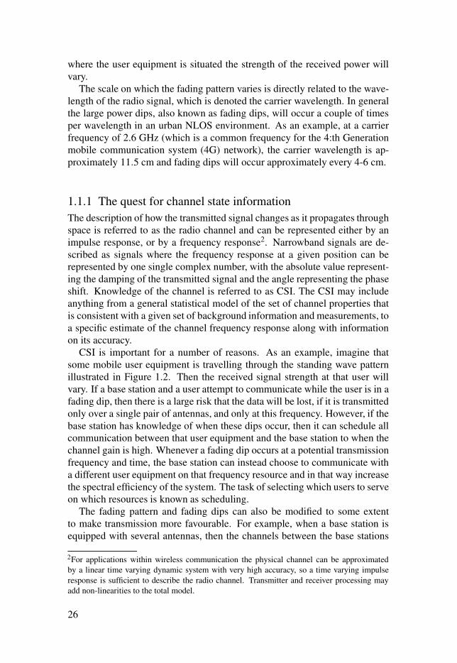
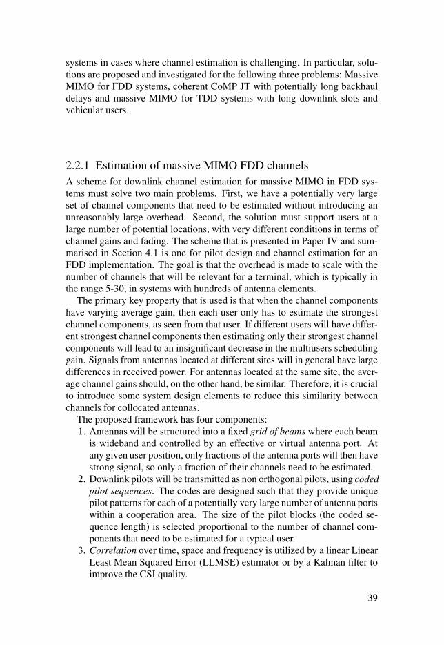
2.2 Kalman filters for potential 5G applications . . . . . . . . . . . . . . . . . . . . . . . . . . . . . . . . 382.2.1 Estimation of massive MIMO FDD channels . . . . . . . . . . . . . . . . 392.2.2 Channel prediction to overcome backhaul delays in

coordinated multipoint systems . . . . . . . . . . . . . . . . . . . . . . . . . . . . . . . . . . . . . . 402.2.3 Channel smoothing for TDD systems with predictor

antennas . . . . . . . . . . . . . . . . . . . . . . . . . . . . . . . . . . . . . . . . . . . . . . . . . . . . . . . . . . . . . . . . . . . . . . . . . . . . 41

3 The Kalman filter . . . . . . . . . . . . . . . . . . . . . . . . . . . . . . . . . . . . . . . . . . . . . . . . . . . . . . . . . . . . . . . . . . . . . . . . . . . . . . . . . . . . . . . 443.1 Background and related work . . . . . . . . . . . . . . . . . . . . . . . . . . . . . . . . . . . . . . . . . . . . . . . . . . . . . . . . 443.2 Mathematical background . . . . . . . . . . . . . . . . . . . . . . . . . . . . . . . . . . . . . . . . . . . . . . . . . . . . . . . . . . . . . 45

3.2.1 Predictions and smoothing . . . . . . . . . . . . . . . . . . . . . . . . . . . . . . . . . . . . . . . . . . . . . . 483.2.2 Comments on complexity and the use of stationary

filters . . . . . . . . . . . . . . . . . . . . . . . . . . . . . . . . . . . . . . . . . . . . . . . . . . . . . . . . . . . . . . . . . . . . . . . . . . . . . . . . . 493.3 Model estimation . . . . . . . . . . . . . . . . . . . . . . . . . . . . . . . . . . . . . . . . . . . . . . . . . . . . . . . . . . . . . . . . . . . . . . . . . . . . 50

3.3.1 Estimation of the parameters of the state spacematrices of one channel element . . . . . . . . . . . . . . . . . . . . . . . . . . . . . . . . . . . . 52

3.3.2 Modelling the correlation between channelcomponents . . . . . . . . . . . . . . . . . . . . . . . . . . . . . . . . . . . . . . . . . . . . . . . . . . . . . . . . . . . . . . . . . . . . . . 53

3.4 Limitations of predictability . . . . . . . . . . . . . . . . . . . . . . . . . . . . . . . . . . . . . . . . . . . . . . . . . . . . . . . . . . 543.4.1 The effects of noisy training data . . . . . . . . . . . . . . . . . . . . . . . . . . . . . . . . . . . 563.4.2 The effects of model order and measurement noise . . . . . . 583.4.3 The effect of the amount of available training data . . . . . . . 58

3.5 Design choices . . . . . . . . . . . . . . . . . . . . . . . . . . . . . . . . . . . . . . . . . . . . . . . . . . . . . . . . . . . . . . . . . . . . . . . . . . . . . . . . 623.5.1 Pilot signal design and the use of coded non

orthogonal pilots . . . . . . . . . . . . . . . . . . . . . . . . . . . . . . . . . . . . . . . . . . . . . . . . . . . . . . . . . . . . . . 623.5.2 Joint estimation of channels at adjacent subcarriers . . . . . 653.5.3 Where to position the filters and the feedback overhead

in FDD systems . . . . . . . . . . . . . . . . . . . . . . . . . . . . . . . . . . . . . . . . . . . . . . . . . . . . . . . . . . . . . . . 65

4 Applications . . . . . . . . . . . . . . . . . . . . . . . . . . . . . . . . . . . . . . . . . . . . . . . . . . . . . . . . . . . . . . . . . . . . . . . . . . . . . . . . . . . . . . . . . . . . . . . 674.1 Channel estimates with non orthogonal pilots for massive

Multiple-Input Multiple-Output (MIMO) Frequency DivisionDuplex (FDD) systems . . . . . . . . . . . . . . . . . . . . . . . . . . . . . . . . . . . . . . . . . . . . . . . . . . . . . . . . . . . . . . . . . . 674.1.1 Relations to previous results . . . . . . . . . . . . . . . . . . . . . . . . . . . . . . . . . . . . . . . . . . . 704.1.2 System design . . . . . . . . . . . . . . . . . . . . . . . . . . . . . . . . . . . . . . . . . . . . . . . . . . . . . . . . . . . . . . . . . . 714.1.3 Results and conclusions . . . . . . . . . . . . . . . . . . . . . . . . . . . . . . . . . . . . . . . . . . . . . . . . . . 74

4.2 Channel prediction for coordinated multipoint jointtransmission . . . . . . . . . . . . . . . . . . . . . . . . . . . . . . . . . . . . . . . . . . . . . . . . . . . . . . . . . . . . . . . . . . . . . . . . . . . . . . . . . . . . 794.2.1 Background and related work . . . . . . . . . . . . . . . . . . . . . . . . . . . . . . . . . . . . . . . . . 824.2.2 Robust linear precoding design and user grouping . . . . . . . 864.2.3 Handling backhaul limitations . . . . . . . . . . . . . . . . . . . . . . . . . . . . . . . . . . . . . . . . 93

4.3 Channel smoothing for TDD systems with predictor antennas . . 964.3.1 History of the predictor antenna concept . . . . . . . . . . . . . . . . . . . . . . . 974.3.2 Kalman smoothing for Time Division Duplex (TDD)

downlink estimates . . . . . . . . . . . . . . . . . . . . . . . . . . . . . . . . . . . . . . . . . . . . . . . . . . . . . . . . . . 984.3.3 Important results and conclusions . . . . . . . . . . . . . . . . . . . . . . . . . . . . . . . . 100

5 Conclusions . . . . . . . . . . . . . . . . . . . . . . . . . . . . . . . . . . . . . . . . . . . . . . . . . . . . . . . . . . . . . . . . . . . . . . . . . . . . . . . . . . . . . . . . . . . . . . 105

References . . . . . . . . . . . . . . . . . . . . . . . . . . . . . . . . . . . . . . . . . . . . . . . . . . . . . . . . . . . . . . . . . . . . . . . . . . . . . . . . . . . . . . . . . . . . . . . . . . . . . . 108

Abbreviations

4G 4:th Generation mobile communication system. 26, 28, 29, 67, 68, 795G 5:th Generation mobile communication system. 23, 28, 29, 34, 38, 42, 67

AR Autoregressive. 37, 38, 45, 46, 50–55, 57–60, 77, 101, 102, 105ARMA Autoregressive Moving Average. 53

CDF Cumulative Distribution Function. 64, 75, 91–94CIR Channel Impulse Response. 71CoMP Coordinated MultiPoint. xix, xx, 23, 34, 35, 37, 39–41, 48, 65, 67, 69,

71, 75, 77, 79–86, 88, 91, 96, 105, 106CQI Channel Quality Index. 28, 65, 88, 89CSI Channel State Information. xix, 23, 26, 28, 34, 37, 39–42, 67, 68, 70, 73,

78, 79, 81–85, 91–95, 97, 99CU Control Unit. 40, 79, 83, 95

DPC Dirty Paper Coding. 83

FDD Frequency Division Duplex. xiv, xx, 28, 29, 39, 42, 61, 64–71, 76, 81,84, 97, 98, 105

GPS Global Positioning System. 97

IoT Internet-of-Things. 23ISI Inter-Symbol Interference. 27

JB Joint Beamforming. 40, 81JS Joint Scheduling. 40, 81, 82, 85JT Joint Transmission. 23, 34, 35, 37, 39–41, 48, 65, 67, 69, 80–85, 88, 91,

106

LLMSE Linear Least Mean Squared Error. xxi, 39, 73–76, 105LOS Line-Of-Sight. 24, 42, 53, 55, 98, 100, 103LTE Long Term Evolution. 29, 34, 67, 74

MIMO Multiple-Input Multiple-Output. xiv, xx, 23, 27, 28, 32, 37–41, 44,61, 64, 66–70, 76, 77, 81–84, 86, 89, 97, 98, 105

MISO Multiple-Input Single-Output. 84ML Maximum Likelihood. 46, 52, 53MMSE Minimum Mean Squared Error. xix, 33, 41

MRC Maximum Ratio Combining. 40, 68, 71–73, 77MSE Mean Squared Error. 33–35, 41, 46, 47, 49, 84, 85, 87, 96

NLOS Non-Line-Of-Sight. 24–26, 38, 42, 55, 74, 98, 100, 103NMSE Normalized Mean Squared Error. xix, xxi, 40, 56–60, 76, 91, 92,

98–100, 102–105

OFDM Orthogonal Frequency Division Multiplexing. 27, 28, 37, 44, 45, 56,68, 71, 76, 86, 98, 99

RAN Radio Access Network. 81, 82

SINR Signal to Interference and Noise Ratio. 68SISO Single-Input Single-Output. 67SNR Signal to Noise Ratio. 28, 56–59, 71, 76, 77, 89, 100, 102, 103

TDD Time Division Duplex. xiv, xxi, 28, 29, 39, 42, 43, 48, 68, 69, 97–100,102, 104, 107

Acknowledgements

There are a large number of people who deserve to be thanked and acknowl-edged in this thesis, these include, but are not limited to, those mentionedbelow.

First and foremost, I wish to thank supervisors Mikael Sternad and AndersAhlén, because without them, this thesis would not have existed. Thank youfor providing me with a place in the research group. A special thanks to Mikaelfor your support, guidance and enthusiasm.

To our secretary Ylva Johansson, thank you for making sure things runsmoothly around the office.

To everyone in the Signals and Systems group, the CORE group and theFTE group, whom I have had the privilege to share my work days with. Thankyou for making my days brighter. A special thank you to Simon, who hasput up with sharing an office with me, to Steffi for her willingness to alwaysdiscuss teaching with me and to Joachim with whom I’ve had the joy to workin projects during these past years.

Over the years I have had enjoyed working with people from the industryand from other universities. Some of these deserve a special mention. So toJingya Li, Tilak Lakshamana and Nima Jamaly from Chalmers Technical Uni-versity, Annika Klockar from Karlstad University, Michael Grieger, RichardFritzsche and Fabian Diehm from TU Dresden, Konstantinos Manolakis fromTU Berlin, Wolfgang Zirwas from Nokia Bell Labs and Dinh Thuy Phan Huyfrom Orange, thank you for enjoyable collaborations and to Tommy Svenssonfrom Chalmers Technical University, thank you for all the advise you haveprovided me with.

To my family, thank you for all your love, support and encouragement. Aspecial thank you to my parents and my in-laws who have been especiallyhelpful babysitting these past months. To my lovely boys Kasper and Alexan-der I wish to thank you for filling my life with joy and to my husband Senad,thank you for always being there for me and loving me even when I’m at myworst.

Finally, to you, the reader. Whether you read the whole thing, skim throughthe next few chapters or only pay attention to the acknowledgements and per-haps a couple of the pictures. Thank you for your time, I hope you enjoy.

Rikke Apelfröjd

Summary of papers

When writing this thesis as a comprehensive summary, the aim has been toexplain the general idea behind different concepts and to highlight those re-sults that are of importance for further study of the subject and results thatmay be of importance as input to standardization of future generations mobilecommunication systems. Technical details such as most equations, proofs andsimulation settings are found in the papers.

As a recommendation, the reader should focus on the extensive summaryin Chapters 1-5 and dive into the details of the papers whenever entering atopic that is of extra interest to the reader. It is then not necessary to read theintroductions of the papers, as this is mainly covered by the comprehensivesummary.

In order to give an overview for those readers who may not be familiar withthe area of wireless communication, Chapter 1 is kept on a very basic levelreviewing some important aspects for the physical layer of wireless communi-cation systems and the basic idea behind estimation theory. As a consequence,any reader familiar with these concepts may want to skip straight ahead to Sec-tion 2.

In terms of the included papers, denoted I-V, there is some overlap whenit comes to the description of the channel models and the Kalman filter equa-tions. The summary below is provided to guide the reader and to highlight themain points of the papers.

Comments of the author’s contributions to each paper with multiple authorsare stated below for each of the five included papers.

Paper I: Kalman predictions for multipoint OFDM downlinkchannelsThis technical report provides a detailed description on how to use the Kalmanfilter for predicting small scale fading of channels. It extends the framework ofthe Ph.D. thesis [1] by Aronsson to include also channels from multiple basestation sites.

Design choices, such as where to locate the filters, how to estimate thechannel models and which pilot pattern to use, are discussed.

The report also includes results on the predictability of small scale fadingmodels. It illustrates how the predictability of a channel is fundamentallylimited by the fading statistics, represented by the Doppler spectrum.

The measurement based prediction results of Paper II and of [2] are high-lighted and studied in detail. Some additional Normalized Mean Squared Er-ror (NMSE) prediction statistics results that where not included in Paper IIare included in this report to highlight different aspects of the prediction per-formance. Based on these performance results, system design issues, such aspilot patterns, intercluster interference and system delays, are discussed in theconclusion section.

The report also includes an appendix on how to generate block-fading chan-nel models that have (instantaneous) error statistics that correspond to the oneobtained in a given physical setting when Kalman predictors are applied. Thismethod has been used in [3].

Paper II: Design and measurement based evaluations of coherentJT CoMP: A study of precoding, user grouping and resourceallocation using predicted CSIThis paper investigates if Coordinated MultiPoint (CoMP) gains are realis-tic in real systems. The evaluations are based on measured channels, withKalman prediction and a robust linear precoder. The linear precoder is basedon a robust Minimum Mean Squared Error (MMSE) design that takes channeluncertainties into account when designing beamforming weights and uses anad hoc method to maximizing a sumrate criterion iteratively.

The Kalman predictions provide Channel State Information (CSI) that issufficiently accurate to achieve significant CoMP gains, even for long temporalprediction horizons (of 24 ms) at pedestrian mobility and at 2.66 GHz. Forshorter prediction horizons (of 5 ms) and at 500 MHz, they would even providegood CSI at vehicular velocities.

Results show that the robustness of the proposed precoder, i.e. the fact thatit takes the CSI uncertainty into account in the precoder design, provides anincrease in sumrate, especially when users are randomly grouped.

Based on results of [4], which showed that user grouping is important tosecure CoMP gains (compared with single cell transmission) this paper inves-tigates different user grouping strategies. In particular, a strategy based onlocal scheduling, over the different resources, is suggested. It is comparedboth with the optimal user groups, found through a very high dimensionalsearch of all possible combinations, and with a greedy user grouping schemesuggested in literature. The here proposed user grouping scheme performs, interms of sum-rate, close to the optimal scheme and to the greedy scheme, at amuch lower complexity.

Interestingly, the results also shows that, for a small CoMP cluster (includ-ing three single antenna base stations) when users are grouped through thesuggested user grouping scheme, then the zero forcing precoder achieves sim-ilar CoMP gains as the proposed robust linear precoder.

The reader who has read Paper I can skim through Sections 2-3 and 6.3 aswell as Appendix A.

The author has done the majority of the work.

Paper III: Robust linear precoder for coordinated multipoint jointtransmission under limited backhaul with imperfect CSIIn this paper the robust linear precoder that is proposed in Paper II is extendedto handle constraints on backhaul capacity. The aim is to ensure that the lossesin CoMP gains, due to less backhaul capacity, are decreased by avoiding to de-sign the precoder under the faulty assumptions that all channels can be used.The suggested solution is to include the backhaul constraints in the minimiza-tion criterion, via penalty terms.

Results show that if the backhaul constraints are handled as suggested, thenthe loss in CoMP gains is lower than if the constraints on backhaul capacityare not considered in the precoding design. The difference in loss is espe-cially high for cell edge users, which are the users that need CoMP most andtherefore have the most to loose from backhaul constraints.

The reader who has read Paper II can skim through Sections 2-3.1 and Ap-pendix A.

The author has done the majority of the work.

Paper IV: Joint reference signal design and Kalman/Wienerchannel estimation for FDD massive MIMOIn this paper, a strategy to use non orthogonal, coded, pilots in order to de-crease the overhead problem that comes with deploying massive MIMO in anFDD system is proposed. It is based on a framwork suggested by Zirwas,Amin and Sternad [5].

The aim is to obtain a large reduction in the pilot overhead, as compared toorthogonal pilots, in downlinks of systems that may use both massive MIMOand CoMP. The general principle behind the proposed pilot design is basedon that only a limited number of channel components are strong, as seen for aperspective from a single user. As channels from antennas located at the samebase station tend to have equal strength, a design elements must be introducedto ensure this basic property. In Paper IV this is achieved by introducing a fixedgrid of beams which directs the transmitted power into different directions,hence causing different channel gains at the user.

The proposed pilot code design is such that any user within the system willbe able to estimate up to its K strongest channel components, where K is thenumber of available pilots. It has the benefit that it does not need to be re-optimized whenever a new user enters the system.

The performance in terms of channel estimation NMSE is evaluated basedon Linear Least Mean Squared Error (LLMSE) filtering and Kalman filtering.A non optimal reduced Kalman filter which only estimates the relevant channelcomponents (which are the strongest channel components at a specific users)is proposed in order to limit the computational complexity, and is evaluated.

System simulation results, in a cluster of nine base stations, show that thechannel NMSE with coded non orthogonal pilots becomes around 5 dB worsethan when using orthogonal pilots, at a much reduced pilot overhead. Theresulting performance degradation becomes insignificant if maximum ratiotransmit beamformers are designed based on channel estimates with the at-tained quality.

The reader who has read Paper I can skim through Sections 3.2 and appen-dices C.2-D.

The simulation environment, which is based on an open source environ-ment developed by the Fraunhofer Heinrich Hertz institute [6], was created incollaboration with Wolfgang Zirwas. The author is responsible for simulatingpilots measurements and implementing the different estimations algorithms,while Zirwas designed the parts relating to simulations of the radio channelsand designing the fixed grid of beams.

Paper V: Kalman smoothing for irregular pilot patterns; A casestudy for predictor antennas in TDD systemsIn this paper the Kalman filter is used to obtain smoothed interpolation esti-mates of the downlink channels of a TDD system, based on uplink channelestimates.

In order to perform smoothing, future measurements of the channel need tobe available to the filter. This can be achieved for vehicular user equipmentby placing an antenna, a predictor antenna, in front of a second antenna, themain antenna, on the roof of a vehicle in the direction of travel. The predictorantenna will then experience the channel before the main antenna and canhence collect "future" measurements of the channel for the main antenna.

Interpolation of the uplink channel needs to be performed over the durationof downlink slots, in which no uplink pilots are available. The quality of theinterpolation performance influence the quality of the channel estimates of thedownlink slots on which downlink transmission and beamforming is based.A good interpolation scheme will allow a longer downlink slot duration to beused for mobile users.

Evaluations based on measurements show that interpolation through Kalmansmoothing of the downlink channels helps to improve the channel estimatesuch that the downlink slots can have durations that correspond to 0.6-0.7 ofthe carrier wavelength in space. If channels are only extrapolated, then this isreduced to 0.2-0.3 of the carrier wavelength.

The work of this paper was carried out in close collaboration with JoachimBjörsell who has been responsible for pre processing of the measurements,while the author has been responsible for the calculations and simulations re-garding the smoothing algorithm.

1. Introduction

Since the shift of the millennia wireless communication has moved frommainly supporting phone calls and occasional data transmission to and frommobile user devices to support large data rates including tracking data, cloudservices and streaming services. The customers of today’s wireless commu-nication systems require constant connection and are not satisfied when datarates drop. Especially not during the commute to work.

The increasing demands require wireless transmission systems that can sup-port a large number of data hungry users that may be densely located and/ortravelling at high velocities. In addition, it is very likely that future wirelesssystems need to support not only the traditional devices that are directly con-trolled by a user such as a mobile phone or a computer, but also more or lessautonomous devices that communicate amongst each other, the so called In-ternet-of-Things (IoT), causing the number of user equipment to increase.

In order for future systems to support both user equipments with high datademands and user equipment with low latency demands, a flexible systemstructure that supports a large number of transmission techniques is required.Strategies for improving spectral efficiency that are currently a part of the instandard include Multiple-Input Multiple-Output (MIMO) transmission, chan-nel information based scheduling and adaptive modulation and coding. Can-didate techniques for future standardization include Coordinated MultiPoint(CoMP) Joint Transmission (JT) and massive MIMO. All these techniqueshave in common that they need accurate Channel State Information (CSI)available at the transmitter side. The estimation of such CSI is crucial forhigh data throughput, however it is important that the quest for accurate CSIdoes not come at the cost of not being able to support bursty traffic.

The work presented in this thesis will focus on evaluating methods to obtainthe CSI required for CoMP JT and massive MIMO, and highlighting resultsthat can be of interest when designing 5:th Generation mobile communicationsystem (5G) networks.

1.1 The radio channelA traditional wireless communication system consists of one or more station-ary base stations that transmit and receive data to and from a large numberof user equipments. Some of the user equipments are mobile, while othersare stationary. The base station (and sometimes the user equipment too) will

23

generally have multiple antennas. These can be used to increase the proba-bility of success (by transmitting or receiving the same message over multipleantennas) or to direct the transmitted or received signal energy.

When a radio signal is transmitted, whether it is directed or is sent out om-nidirectional, the energy of the signal will spread. A bit simplified, this canbe described as the information carrying sinusoidal radio signal splitting upin multiple rays that each propagates into a different direction and interactswith the environment through reflection, refraction and by loosing energy tothe medium that it travels through. An illustration of this is shown in Fig-ure 1.1. Here, a radio signal is transmitted to a mobile phone (a piece of userequipment) on ground level from a base station situated on the roof of a tallbuilding. Only a very small fraction of the transmitted radio frequency powerwill reach the intended destination. Figure 1.1 illustrates some of the paths ofthe radio waves that reach the mobile. The signal can be modelled as multiplerays (which in the example are reduced to four rays to make them easily dis-tinguished) 1. One of these rays refracts over the roof of the building and thentakes a direct route to the phone, while the other rays travel in different direc-tions and reflect one or more times on buildings before reaching the phone.As the figure illustrates, the rays that travel a longer way are weaker once theyreach the mobile phone, and the one ray that is reflected from the rooftop ofone of the low buildings has its strength further weakened due to the radiosignals propagation through vegetation.

Any part of the radio signal that reaches the receiver in a straight path fromthe transmitter (without having reflected or refracted on the path) is called aLine-Of-Sight (LOS) component, whereas any part of the radio signal thathas had its direction changed during the propagation to the receiver is calleda Non-Line-Of-Sight (NLOS) component. Similarly, a channel with a strongLOS component and only weak NLOS components is called a LOS channeland a channel with a relatively insignificant LOS component is called a NLOSchannel.

The multiple rays in Figure 1.1 will add up either constructively or destruc-tively at the mobile user depending on the relative phase shifts of the sinu-soids. As the phase shifts depend on the lengths of the paths each componenthas travelled, the received power will differ for different locations in space.Figure 1.2 shows an illustration of how the strength of a radio channel maylook in space for a typical NLOS channel when the signal transmitted is nar-rowband, i.e. when it spans a small frequency interval. The standing wavepattern that appears is referred to as a small scale fading pattern. In a LOSscenario, the fading pattern will in general be much smoother. Depending on

1This "ray tracing" way of modelling radio wave propogation is an approximation of the exactsolution, which would be obtained by solving Maxwell’s equations within exactly known andspecified boundary conditions.

24

Figure 1.1. An illustration of a multipath channel. The strength of the radio signal atdifferent points in space is indicated by the intensity of the color and the dashed lineindicates a significantly weaker strength.

Figure 1.2. An illustration of a standing spatial wave pattern of a typical scalar urbanNLOS narrowband channel. The received energy on the horizontal plane of a signaldepends on the spatial location of the user equipment.

25

where the user equipment is situated the strength of the received power willvary.

The scale on which the fading pattern varies is directly related to the wave-length of the radio signal, which is denoted the carrier wavelength. In generalthe large power dips, also known as fading dips, will occur a couple of timesper wavelength in an urban NLOS environment. As an example, at a carrierfrequency of 2.6 GHz (which is a common frequency for the 4:th Generationmobile communication system (4G) network), the carrier wavelength is ap-proximately 11.5 cm and fading dips will occur approximately every 4-6 cm.

1.1.1 The quest for channel state informationThe description of how the transmitted signal changes as it propagates throughspace is referred to as the radio channel and can be represented either by animpulse response, or by a frequency response2. Narrowband signals are de-scribed as signals where the frequency response at a given position can berepresented by one single complex number, with the absolute value represent-ing the damping of the transmitted signal and the angle representing the phaseshift. Knowledge of the channel is referred to as CSI. The CSI may includeanything from a general statistical model of the set of channel properties thatis consistent with a given set of background information and measurements, toa specific estimate of the channel frequency response along with informationon its accuracy.

CSI is important for a number of reasons. As an example, imagine thatsome mobile user equipment is travelling through the standing wave patternillustrated in Figure 1.2. Then the received signal strength at that user willvary. If a base station and a user attempt to communicate while the user is in afading dip, then there is a large risk that the data will be lost, if it is transmittedonly over a single pair of antennas, and only at this frequency. However, if thebase station has knowledge of when these dips occur, then it can schedule allcommunication between that user equipment and the base station to when thechannel gain is high. Whenever a fading dip occurs at a potential transmissionfrequency and time, the base station can instead choose to communicate witha different user equipment on that frequency resource and in that way increasethe spectral efficiency of the system. The task of selecting which users to serveon which resources is known as scheduling.

The fading pattern and fading dips can also be modified to some extentto make transmission more favourable. For example, when a base station isequipped with several antennas, then the channels between the base stations

2For applications within wireless communication the physical channel can be approximatedby a linear time varying dynamic system with very high accuracy, so a time varying impulseresponse is sufficient to describe the radio channel. Transmitter and receiver processing mayadd non-linearities to the total model.

26

antennas and an antenna at the user equipment will have different (althoughin general correlated) fading patterns. If the base station is aware of the phaseshifts of each channel, then it can adjust the phase shifts of the radio signalsfrom each transmit antenna to ensure that these will add up constructivelyat the user equipment, thus lowering the depth and the spatial density of thefading dips and improve the overall channel gain.

Similarly, when the user equipment transmits a radio signal to the basestation, the receiver can weight and combine measurements from differentantennas to improve the quality of the received signal.

These are only a few examples of MIMO techniques that not only can in-crease the data throughput, but also can allow a base station to transmit si-multaneously to many users within the same frequency bands. The latter isenabled by adjusting the resulting standing wave pattern of the received sig-nals at each user’s location such that only the part of the transmitted signalintended for that particular user will be added up constructively and thus havea high receive power, while the parts of the transmitted signal that are intendedfor other users are left non-amplified, or are made to add up destructively.

1.1.2 Orthogonal frequency division multiplexing: A briefoverview

In an Orthogonal Frequency Division Multiplexing (OFDM) system a broad-band signal is created as several narrowband signals that are superpositionedinto one time limited signal, denoted one OFDM symbol, before being trans-mitted over the radio channel. Each of these narrowband signals, often referredto as subcarriers, can then be used to encode separate pieces of information, ormessages. By adjusting the frequency band of the narrowband signals basedon the time duration of the OFDM symbol, modulated narrowband signalscan be made orthogonal over the symbol time such that, under ideal assump-tions, the messages encoded on different subcarriers will not interfere witheach other. Under realistic assumptions, the system and receiver can be de-signed to ensure that interference between subcarriers is very small, if thetransmitter and receiver are synchronized in time and frequency with suffi-cient accuracy. Likewise, the system is often designed to ensure that interfer-ence between subsequent OFDM symbols in time, Inter-Symbol Interference(ISI), can be considered negligible.

In an OFDM system, a single subcarrier over the duration of a single OFDMsymbol is referred to as a time-frequency resource or simply resource. Just asthe channel changes over time, it may also change over frequency. A channelcan either be flat fading, with constant channel gain (although different phase)over all subcarriers, or it can be frequency selective, in which case the gainvaries over different subcarriers. At the base station, a scheduling algorithmwill be used to assign resources to each user equipment within the system.

27

Most utilized scheduling algorithms are based on some CSI, which may con-sist of the complex-valued channel gains or simply a Channel Quality Index(CQI). The CQI may include information of the Signal to Noise Ratio (SNR)of the subcarrier, or simply information on which subcarriers have channelsthat are above a given SNR threshold. The scheduler will aim to schedulemessages on the resources where the channels of a user are good.

The time and frequency spread of a resource is often designed to ensure thatthe channel associated with it can be described by a single complex-valuedscalar h. Likewise, the part of the transmitted and received signals that areassociated with the time-frequency resource can also be described by complex-valued scalars, here denoted s and y respectively. The received message canthen be described as the product of the transmitted signal and the channelwith some additional additive noise and interference. If multiple users will bescheduled on the same resource, then multiuser MIMO techniques are used toensure that each user equipment receives the messages intended for it. Suchtechniques will be further discussed in Chapter 4.

For further reading on the topic of OFDM the interested reader may referto e.g. the works of [7], which gives a thorough theoretical background tothe topic, [8], which explains the implementation of OFDM in the current 4Gsystem, and [9] which describes the implementation of OFDM in the future5G system.

1.1.3 Uplink and downlinkThe radio channel of radio systems that have a fixed infrastructure of base sta-tions is separated into uplink and downlink. Over the uplink, the user equip-ment transmits information to the base station and over the downlink the basestation transmits information to the user. By using different resources for up-link and downlink, strong self-interference, i.e. that the weak received signalis interfered by its own strong transmitted signal, on the same time/frequencyresources, is eliminated.

The amount of resources that are allocated to uplink and downlink respec-tively is a design choice that depends on how much information that is an-ticipated to be transmitted over each link. As surfing and streaming servicesbecome more common, it is likely that the uplink will be allocated less re-sources than the downlink as illustrated in Figure 1.3.

There are two common ways of separating uplink and downlink, both ofwhich are illustrated in Figure 1.3. In FDD systems, uplink and downlinktransmit simultaneously but in different frequency bands, whereas in TDD,the full bandwidth is utilized for both uplink and downlink, however the twoare separated in time.

These designs both have their advantages and disadvantages. For example,as the frequency response of the channel varies in different bands, separate

28

Figure 1.3. Uplink and downlink resource allocation for FDD and TDD systems re-spectively.

channel estimations are required for uplink and downlink in FDD systems. Incontrast, in TDD systems the uplink and downlink frequency responses willgenerally be similar for the same position in space - with some differences dueto using different transmit and receive filters in the two links, which will intro-duce differences due to hardware imperfections in the equipment. This prop-erty is called channel reciprocity. On the other hand, low latency requirementscould be easier to handle in an FDD system. If, for example, an automaticcontrol system needs a small piece of data within a short time frame, but thesystem has just switched to an uplink slot, then there is a good chance that theinformation will be invalid by the time the system reaches its downlink slot.A potential remedy is to create flexible uplink downlink slots where users thathave low latency demands may have very short switching times between up-links and downlink. However this does place higher flexibility demands on thesystem and will create increased interference between different nodes.

The current 4G Long Term Evolution (LTE) systems are based on FDDwith exception of the Chinese 4G LTE which is based on TDD. The pairedspectral bands currently used for 4G and earlier systems will likely remainFDD spectra for a foreseeable future, whereas any new spectra that will beused for 5G systems will most likely mainly be TDD based, with a flexibleuplink/downlink slot allocation, in order to adjust the resources depending onapplication.

1.2 Channel estimationIn order to estimate the channel required for, e.g., resource scheduling andtransmission design, some resources are reserved for the base station and/oruser equipment to transmit pilot signals. These are signals that are known toboth the user and the base station. By measuring the received signal within apilot resource, the channel frequency response can be estimated.

As a very simple example, consider a sinusoidal signal where informationbits are coded into the amplitude and phase shift (with respect to some refer-ence time) which are represented by the absolute value and a phase angle re-

29

spectively, of the complex number s, called a symbol. Furthermore, considerthat this signal is transmitted through a time-invariant narrowband channel,where the complex-valued frequency response of the channel h describes howthe amplitude and the phase of the transmitted signal is altered during propaga-tion through the channel. Then the amplitude and phase of the received signalcan be represented by the absolute value and the phase angel respectively of acomplex-valued number yd where

yd = hs.

Now assume that prior to transmitting the bits represented by s, a pilot signalwith the same frequency as the sinusoid carrying information bits was trans-mitted. We let the complex-valued p represent the known phase and amplitudeof the transmitted pilot signal and yp = hp represent the amplitude and phaseof the received pilot signal. As the pilot is known at both transmitter and re-ceiver, it can be used to find the channel through the relation h = yp/p, and byextension also the transmitted signal on the receiver side through

s =yd

yp

p.

The example above gives the basic reasoning behind pilot-based channelestimation. However it is not an accurate representation of reality. In a morerealistic scenario both the pilot measurements and the received data symbolyd will be subjected to noise, both from the hardware equipment and frominterfering signals from other transmissions e.g. from neighbouring frequencybands and/or from neighbouring transmitters. In addition, the channel may notbe static. In particular, if the user equipment is mobile, then the channel thataffects the pilot signal will differ from the channel that the data carrying signalexperiences to some extent depending on the user mobility, the fading pattern(Figure 1.2) and the time delay between the two signals.

A more general way to approximate the pilot measurement at a single re-ceive antenna is through

yτ = Φτhτ +nτ . (1.1)

Here yτ and nτ are complex-valued column vectors of dimension K consistingof measurements and measurement noise respectively during a time windowindexed by an integer τ . Each element in these represent a separate set ofmeasurement and measurement noise, e.g. from different subcarriers. Theelements of the complex-valued channel column vector hτ of dimension Ntx ·Krepresent the channel frequency responses from the Ntx transmit antennas atthe K time-frequency locations of the measurements. The K ×Ntx ·K matrixΦτ is filled with pilot symbols that represent all the signals transmitted on eachantenna over each of the K resources.

The problem of channel estimation is the problem of finding an estimatehτ+m of the channel vector at a time window indexed by τ +m using as much

30

of the available information about the noise nτ , the measurement yτ , the pilotmatrix Φτ and the relationship between the channel vectors hτ and hτ+m asrealistically possible. In addition to the exact values of the pilot matrix andchannel measurements, the available information often consists of first andsecond order statistics, i.e. mean values, covariance matrices and autocorrela-tion functions. Often there are also past channel measurements available.

1.2.1 Pilot designThe expression (1.1) is flexible as it allows us to choose the structure of thepilots. Three different types of pilot designs will be considered throughoutthis thesis.

Resource orthogonal pilots

Resource orthogonal pilots means that each transmit antenna is allocated in-dividual time-frequency resources to transmit pilots. When a pilot resourceis allocated to one antenna every other antenna must be silent. This patterncreates no inter-antenna interference.

An example with K = 2 and Ntx = 2 is

[y1y2

]=

[1 0 0 00 0 0 1

]⎡⎢⎢⎣h11h12h21h22

⎤⎥⎥⎦+

[n1n2

], (1.2)

where hi j is the channel at resource i from antenna j. Thus, antenna 1 sendsits pilots only in resource 1 and antenna 2 sends its pilot only in resource 2.We may here directly obtain the channel estimates

h11 = y1 = h11 +n1,

h22 = y2 = h22 +n2.(1.3)

We obtain no direct measurement of h12 and h21, but assuming that the channelfrom one antenna is equal to all the K transmission resources, we may use theestimates

h12 = h11 = y1

h21 = h22 = y2.(1.4)

Code orthogonal pilots

Code orthogonal pilots allow more than one antenna to transmit pilots on thesame pilot resources. However, the structure of the pilots are such that a se-quence of pilots transmitted from one antenna on the given resources is or-thogonal to a sequence of pilots transmitted on the resources by a another

31

antenna. In order to achieve this, the number of available resources must beat least equal to the number of antennas. Use of code orthogonal pilots are ingeneral inferior to resource orthogonal pilots as it creates interference betweenthe antennas on each resource K that cannot in general be fully cancelled atthe receiver.

An example with K = 2 and Ntx = 2 is

[y1y2

]=

12

[1 1 0 00 0 1 −1

]⎡⎢⎢⎣h11h12h21h22

⎤⎥⎥⎦+

[n1n2

], (1.5)

If channels from one antenna are equal in both resources, h11 = h12 = h1 andh21 = h22 = h2, then we have a system with two unknowns and two equations,with unique solution for nk = 0

ˆh1 = y1 + y2,

ˆh2 = y1 − y2.(1.6)

However, in general, if h11 �= h12 or h21 �= h22, we have an under determinedsystem of equations, with no unique solution. We can then not estimate all fourchannels hi j based on measurements at time τ only. If we in such case use the(erroneous) hypothesis h11 = h12 and h21 = h22 to produce the estimates (1.6),then estimation errors will be inevitable even in the noise free scenario.

Non orthogonal pilots

Non orthogonal pilots also allow multiple antennas to transmit on the samepilot resources but without the restriction that the pilot sequences must beorthogonal.

In the example above, the pilot matrix may then be

Φτ =

[p1 p2 0 00 0 p3 p4

], (1.7)

where pi are arbitrary but known complex numbers. Using non orthogonalpilots generally decreases the performance but it comes with the benefit ofreducing pilot overhead, which is important in systems with a large number ofantennas, e.g. massive MIMO systems, where it is desirable to use K < Ntx.

More details and comparisons between the different pilot designs are givenin in Sections 3.5.1, 4.1 and 4.2.

1.2.2 Linear estimationWe saw in the examples above that estimating the channel vector hτ for multi-ple transmit antennas based on pilot measurements yτ at time step τ only will

32

in general represent an estimation problem with more unknowns than con-straints. It is natural to increase the number of constraints by using additionalmeasurements, in particular measurements that were already obtained at pre-vious time steps.

In linear estimation the vector hτ+m is estimated through a weighted sumof all available measurements up to time step τ

hτ+m|τ =τ

∑i=0

Wiyi =[W0 . . .Wτ

]⎡⎢⎣

y0...

yτ

⎤⎥⎦= Wy. (1.8)

Here τ +m|τ is used to denote the estimate of the channel vector at time τ +m

provided measurements up until time τ . The weighting matrices Wi are basedon some or all of the available statistics of the channel and are chosen to mini-mize some criterion. An advantage to linear estimation compared to non-linearestimation is that linear estimation often requires much lower computationalcomplexity.

The most common criterion to minimize in estimation theory is the MeanSquared Error (MSE), i.e.,

E[|hτ+m− hτ+m|τ|2], (1.9)

where | · | is used to represent the euclidean norm of a vector and E[·] denotesthe expected value. It is well known that the optimal solution to the MinimumMean Squared Error (MMSE) problem of finding a linear estimator W in (1.8)that minimizes the MSE (1.9) is given by the causal Wiener filter [10].

For calculating a Wiener filter, a statistical correlation model must be avail-able for the correlation between different elements of the channel vector hτ

in (1.1), and of the noise nτ . By using this correlation information, a uniqueminimum MSE estimate is produced, also in cases as the example (1.6) withh11 �= h12 where a unique exact algebraic solution cannot be obtained.

A disadvantage of the Wiener filter is that finding the weight matrix W in(1.8) requires inversion of the covariance matrix of the vector [yT

0 , ...,yTτ ]

T . Asthis covariance matrix grows with every new measurement, the complexity as-sociated with the matrix inversion will very soon become infeasible, unless wegive up on using all past data, and instead use a limited sliding time window.

To lower the complexity of the estimator, a Kalman filter can instead beused. A Kalman filter is a recursive version of a Wiener filter that utilizes astate space model of the temporal correlation of the channel. The Kalman filterhas the advantage that, for a wide sense stationary system, it will convergesuch that the more computational demanding processing can be calculatedoff-line, and hence the complexity associated with updating the estimate hτ+m

given a new measurement can be kept relatively low [1]. For this reason,the work in this theses is mainly based on the Kalman filter, which will be

33

described in further detail in Chapter 3, with Chapter 4 bringing up potential5G system applications for the filter.

Whether the Kalman or the Wiener filter is used, the statistic of the channel,in the form of covariance matrices and/or autocorrelation functions must be es-timated. Such estimations will always introduce some model errors, which tosome extent destroy the optimality of the filter. A disadvantage to the Kalmanfilter compared to the Wiener filter is that model errors will be introduced intwo steps. First, by estimating the covariance matrices and/or autocorrelationfunctions, and second when using these to estimate a state space model of thechannel. The effect of these model errors on the resulting MSE is discussedfurther in Section 3.4.

1.2.3 Filters, predictors and smoothersDepending on if the integer m in (1.8) is zero, positive or negative, the estimateis called a filter estimate, a prediction or a smoothed estimate respectively. Thedifference between these three is how much measurement data is available, attime step τ +m.

The filter estimate requires measurement data up until the time of the esti-mate. This is useful when the channel has not changed much between the timethe latest pilot measurement was received and the time the channel estimateis used. Let us consider the example presented in Section 1.1 with a carrierwavelength of 2.6 GHz, with users moving at 5 km/h (pedestrian speed) andtime delays of up to 1 ms. As explained above, the dips of Figure 1.2 will thenbe approximately 4-6 cm apart. As a user moves through the standing wavepattern it will have travelled 1.4 mm in the time between receiving the pilotmeasurement and the time of using the channel estimate. Over this short dis-tance, the channel will only have changed slightly, and the estimation errorsdue to this change are generally small, so the filter estimate will suffice formost pedestrian applications. However, for higher velocities or longer timedelays this will not longer be true.

As pilots take up resources that would otherwise be used for data transmis-sion it is of interest to transmit them only when required. For example, inLTE, the CSI reference signals, which are downlink pilots used for estimatingchannels from multiple antennas, are transmitted with an interval of at least5 ms. Delays can also be introduced for other reasons, e.g. in a system withmultiple base stations that are cooperating to transmit messages to the sameusers, through so called CoMP JT. Then information needs to be shared overbackhaul links and this could potentially take up to tens of ms. As the systemdelays increase, the channel will change to a greater extent and the CSI pro-vided by the filter estimate will be outdated. A similar effect is obtained athigher user velocities. In such scenarios predictions are required. Section 4.2

34

focuses on channel prediction for scenarios with long delays and slowly mov-ing users when predictions are used for CoMP JT.

A way of describing the small scale fading of a single narrowband radiochannel hτ , from the perspective from a user that is moving through a stand-ing wave pattern as the one in Figure 1.2, is by the channel’s autocorrelationfunction R(t) = E[hτh∗τ−t ] or by a Doppler spectrum. The Doppler spectrum isgiven by the Fourier transform of the autocorrelation function. The width andshape of the Doppler spectrum affects the predictability of a radio channel.This will be discussed further in Section 3.4.

In order to obtain a smoothed estimate, measurement data from both pastand future, relative to the time of interest, are required. An example when thismay be available is if the receiver is in no rush to detect its signals and can waitfor the next pilot measurement before using all available pilot measurementsto estimate the channel and hence detect the transmitted symbol. A secondapplication for channel smoothing is described in Section 4.3 and includes theuse of a predictor antenna, a concept which will be described briefly in thenext subsection and in more detail in Section 4.3.

The challenge with long range channel prediction and how to solve it

It is intuitive that access to more measurement data also should provide betterestimates. Hence, the smoothed estimate outperforms the filtered estimate interms of MSE and the filtered estimate in turns outperforms the prediction.It is likewise intuitive that the quality of the prediction decreases as the pre-diction horizon m in (1.8) increases. It has been shown in e.g. [1], that aprediction horizon beyond a few tenths of the carrier wavelength in space isinfeasible using linear predictors. The reasons behind this will be exploredmore in Section 3.4.

For a user equipment that moves through a standing wave pattern generatedby a stationary transmit antenna and fixed reflecting or scattering objects, arequired prediction horizon of L seconds is equivalent to a prediction horizonin space in terms of carrier wavelengths

Lv

λ=

Lv fc

c[wavelengths]. (1.10)

where v is the velocity in m/s, λ is the carrier wavelength, c is the speed of lightand fc is the carrier frequency. As an example, at fc = 3.5 GHz predicting 10ms ahead in time would at a velocity of 30 m/s correspond to prediction overa distance of 3.5 wavelengths in space.

A way to push the prediction horizon beyond that of a few tenths of thecarrier wavelength for vehicle users is by utilizing a predictor antenna. Theconcept is illustrated in Figure 1.4. Here, two antennas are positioned on theroof of a bus, aligned along the direction of travel. The forward antenna, whichis denoted the predictor antenna, transmits or receives pilots (depending onthe system). From these pilots, the channel is estimated and this filter estimate

35

Figure 1.4. Illustration of the predictor antenna concept. In this example, a bus isequiped with two antennas aligned along the direction of travel. At a time τ the for-ward antenna, denoted predictor antenna, either transmits or receives a pilot (depend-ing on the system) allowing for a filter estimate of the channel at the location markedby the red square. At the time τ +m the rearward antenna, denoted main antenna,has entered the same location, so the filter estimate based on the prediction antenna attime τ can be used as a channel prediction for the main antenna.

can then be used to design a transmitter that transmits to the rearward antenna,denoted main antenna, at a later time when it has reached the same position inspace as where the predictor antenna was at the time of pilot transmission.

The predictor antenna concept can be used to gain access to future mea-surements of the channel, relative to the position of interest, if the antennasare sufficiently separated. This also allows for a smoothing estimate, basedon the pilots received or transmitted by the predictor antenna, to be used aschannel predictions for the rearward antenna.

36

2. Contributions

For many wireless transmission schemes, accurate CSI at the transmitter of adownlink is crucial to achieve desirable gains. Such schemes include adap-tive modulation and coding [11], channel aware scheduling [12] and multiuserMIMO transmission, e.g. zero forcing, [13].

For this reason, channel estimation has been a topic of interest for wire-less communication for a long time. Particularly, the use of linear filtering isuseful, as it helps to keep computational complexity at bay.

2.1 The Kalman filterKalman estimators and predictors for OFDM MIMO channels, based on Au-toregressive (AR) models for fading statistics, were proposed by Aronssonin [1]. In Paper I and Paper II these methods are extended to multi-antennaand multi-site downlink channels and are evaluated for use in CoMP JT. Anoverview of how to obtain the AR model and the noise covariance matricesthat specify a Kalman filter is given in Paper I, along with discussions of de-sign choices of both the modelling and the Kalman filter.

2.1.1 Factors limiting the predictability of the radio channelsThe Kalman filter can be used not only as a tool for estimation, but also as atheoretical tool for exploring the attainable estimation accuracy under variousassumptions. One such long-standing problem are the basic reasons for thevery limited predictability of fading radio channels that are measured underrealistic conditions. Results based on channel sounding measurements in [14]and in [1] have consistently found that it is in general hard to predict the smallscale fading of a component (either in the time domain or in the frequencydomain) more than a couple of tenths of wavelengths ahead in space.

On the other hand, the physical time varying channel generated by movingthrough a stationary fading environment will be strictly band limited: Thesupport of the Doppler spectrum is constrained to ± the maximum Dopplerfrequency fd = v/λ , where v is the velocity and λ is the carrier wavelength.It is known [15, 16] that strictly band limited signals can be infinitely wellpredictable from past noise free measurements.

If this is the case, then why is it practically impossible to predict fadingchannels over multiple wavelengths? Is it because a predictor is forced to

37

extrapolate based on noisy past channel estimates, or is the fundamental reasonsomething else?

The question of what factors limit the predictability is discussed in Sec-tion 3.4 and in Paper I, using properties of AR modelling and Kalman basedprediction based on AR models.

It turns out that the noise level on past estimates has a relatively small influ-ence on the error of long range channel predictions. The fundamental reasonsfor lack of predictability is instead that finite order models of the fading pro-cess, that are based either on a finite set of training data or on noisy trainingdata, cannot be band limited. This lack of band limitation in the model veryefficiently destroys long-range predictability.

Models based on time limited data sets will essentially see the physicalfading channel through a time window, and this window smears the Dopplerspectrum. Models based on noisy training data will have a noise floor in theirDoppler spectrum. In both cases, the models will lack infinite peaks (puresinusoids) which would theoretically be perfectly predictable.

A starting point for the present investigation are interesting results obtainedby Baddour and Beaulieu [17] on one step prediction errors of AR models offading processes obtained from noisy training data sets.

Here, the method of [17] is used to approximate a band limited theoreticalDoppler spectra for NLOS channels with uniformly distributed scatterers intwo dimensions [18] by a high order AR model that is obtained by addinga small regularization term to the autocorrelation of the channel at zero timeshift. Based on this, various factors that affects the predictability of the radiochannel are evaluated.

Furthermore, results in Section 3.4 abd Paper I show that the measurementnoise associated with the pilot measurements is of less importance than otherfactors when it comes to the range of predictability of a channel. The firstorder effect is the quality of the training data, i.e. how much broadening andsmearing it induces into the Doppler spectrum of the estimated fading model.The second order effect is the model order. When the autocorrelation func-tion of the channel is perfectly known, with except for some white noise thatslightly alters the term to the autocorrelation of the channel at zero time shift inthe same way as the regularization term described above, then a higher modelorder leads to more accurate predictions. However, a too high model order willresult in worse channel estimate whenever the channel statistics changes overtime. Results here supports what was found in [1, 19]; that linear predictionbeyond a couple of tenths of the carrier wavelength has very poor accuracy.

2.2 Kalman filters for potential 5G applicationsIn Chapter 4, linear estimation, and in particular Kalman filtering is used toinvestigate the potential of different MIMO transmission techniques for 5G

38

systems in cases where channel estimation is challenging. In particular, solu-tions are proposed and investigated for the following three problems: MassiveMIMO for FDD systems, coherent CoMP JT with potentially long backhauldelays and massive MIMO for TDD systems with long downlink slots andvehicular users.

2.2.1 Estimation of massive MIMO FDD channelsA scheme for downlink channel estimation for massive MIMO in FDD sys-tems must solve two main problems. First, we have a potentially very largeset of channel components that need to be estimated without introducing anunreasonably large overhead. Second, the solution must support users at alarge number of potential locations, with very different conditions in terms ofchannel gains and fading. The scheme that is presented in Paper IV and sum-marised in Section 4.1 is one for pilot design and channel estimation for anFDD implementation. The goal is that the overhead is made to scale with thenumber of channels that will be relevant for a terminal, which is typically inthe range 5-30, in systems with hundreds of antenna elements.

The primary key property that is used is that when the channel componentshave varying average gain, then each user only has to estimate the strongestchannel components, as seen from that user. If different users will have differ-ent strongest channel components then estimating only their strongest channelcomponents will lead to an insignificant decrease in the multiusers schedulinggain. Signals from antennas located at different sites will in general have largedifferences in received power. For antennas located at the same site, the aver-age channel gains should, on the other hand, be similar. Therefore, it is crucialto introduce some system design elements to reduce this similarity betweenchannels for collocated antennas.

The proposed framework has four components:1. Antennas will be structured into a fixed grid of beams where each beam

is wideband and controlled by an effective or virtual antenna port. Atany given user position, only fractions of the antenna ports will then havestrong signal, so only a fraction of their channels need to be estimated.

2. Downlink pilots will be transmitted as non orthogonal pilots, using coded

pilot sequences. The codes are designed such that they provide uniquepilot patterns for each of a potentially very large number of antenna portswithin a cooperation area. The size of the pilot blocks (the coded se-quence length) is selected proportional to the number of channel com-ponents that need to be estimated for a typical user.

3. Correlation over time, space and frequency is utilized by a linear LinearLeast Mean Squared Error (LLMSE) estimator or by a Kalman filter toimprove the CSI quality.

39

4. Use of cycling sequences of pilot codes ensures good estimations regard-less of the user position, by weighted time averaging of estimation errorsthat may be caused by the non orthogonality of some of the pilot codes,as seen from one user.

System simulations using the Matlab based, open source, Quadriga chan-nel simulator, developed by the Fraunhofer Heinrich Hertz institute [20, 6]show that by using the fixed grid of beams and coded non orthogonal pilots,channel estimations with a reduced Kalman filter provided an average channelestimate Normalized Mean Squared Error (NMSE) of 5 dB worse than whatcould be achieved with resource orthogonal pilots. The resource orthogonalpilots would, however, cause a much higher overhead. The beamforming gainsthrough Maximum Ratio Combining (MRC) were not noticeably affected bythis NMSE reduction.

2.2.2 Channel prediction to overcome backhaul delays incoordinated multipoint systems

There are many challenges and hurdles to overcome before downlink CoMPcan be fully deployed, especially for coherent JT. The work presented in Pa-pers II-III and summarised in Section 4.2 focuses on three of these challenges.

First, data sharing over backhaul links will cause time delays between thechannel estimation and the payload transmission. CoMP decisions will then bebased on outdated CSI. How this affects the potential CoMP gains depends onthe scheme used, i.e. Joint Scheduling (JS), Joint Beamforming (JB) or JT, andon the network architecture, i.e. centralized, distributed or semi distributed,see e.g. [21, 22]. It turns out that the CSI quality is especially important forcoherent JT in a centralized architecture, which is also the solution that wouldprovide the largest potential gains. It is therefore of great importance to findmethods to improve the CSI, under long backhaul delay constraints, in orderto make coherent CoMP JT feasible.

Data sharing over backhaul links places high demands on the backhaul ca-pacity, especially for JT. In realistic systems, these demands may not alwaysbe met. Then the information available at the Control Unit (CU), which is alogical entity that makes the CoMP decisions, will be limited. Furthermore,the possibility to share payload data between the base stations may also belimited. If the CoMP design does not handle these backhaul constraints, thenpotential CoMP gains may be lost.

Second, a nontrivial problem for coherent CoMP is that of which users toserve jointly on each specific transmission resource. If these are selected care-fully then there is a potential for large multiuser diversity gains, as was shownfor multiuser MIMO in e.g. [23, 24]. However the complexity of a searchthrough all possible user groups and all resource allocation possibilities growscombinatorially with the number of users to choose from. It is desirable to

40

have a simple scheme that is low in complexity and that preserves the mul-tiuser diversity gains of the optimal solution.

Third, the messages that are to be transmitted to the users need to be pre-coded to mitigate inter user interference within the cooperation cluster. Ina system with perfect CSI this can be achieved by channel matrix inversion,which provides the zero forcing precoder developed for MIMO, see e.g. [25].However, there is a risk in using zero forcing for CoMP JT, even in the pres-ence of perfect CSI as it is only designed to minimize intracluster interference,but not to weight this against intercluster interference. An option is then to usean MSE criterion which includes these terms as well as the intracluster inter-ference [26].

MSE criteria are attractive as they generally have analytical solutions. How-ever, in practice it is often more useful to maximize over a weighted sumratecriterion, as this is closer to the desired end performance. Such an optimiza-tion poses a multidimensional nonconvex optimisation problem.

The work presented in Papers II-III and summarised in Section 4.2 aims toadress these challenges through three main contributions

1. The problem of the outdated CSI is partly counteracted by channel pre-dictions through Kalman filtering.

2. A very low complexity method for user grouping and resource allocationis proposed and evaluated. This method provides very close to optimalCoMP groups and resource allocation, in the case of the sumrate crite-rion. It places no extra requirements on backhaul capacity.

3. A low complexity robust linear precoder design is proposed. This is arobust MMSE design that offers a flexible tool to optimize over a fewparameters with respect to an arbitrary criterion, e.g. the sumrate. Therobust design takes channel uncertainties due to prediction errors andquantization into account. It can also include backhaul constraints in aflexible way.

For the evaluations, pilot sounding channel measurements collected by Er-icsson in Stockholm have been used. The results show that channel predictionscan ensure CoMP JT performance gains for system delays of tens of milisec-onds at pedestrian speed, or, if the system delays are shorter, then at evenhigher speeds.

2.2.3 Channel smoothing for TDD systems with predictorantennas

For pedestrian users, the required prediction horizon is usually within the 0.1-0.3 carrier wavelength limitation, whereas for high mobility users, a longerprediction horizon is often required.

This limit of prediction horizon can be circumvented by the predictor an-tenna concept, introduced in subsection 1.2.3. It uses an extra antenna, pre-

41

dictor antenna, placed in front of the main antenna, e.g. on the roof of thevehicle, to scout the channel that will later be encountered by the main an-tenna, as originally proposed in [27], see Figure 1.4.

In an FDD system, the predictor antenna would receive known pilots in thedownlink and based on these estimate the channel. If pilots are transmittedoften and the two antennas are sufficiently spaced, then one of these estimatescan be used as a prediction of the channel for the main antenna. However, athigh user velocities, the frequency with which pilots must be transmitted forthe CSI not to be outdated may cause undesirable overhead.

For a TDD system, the predictor antenna would transmit known pilots inthe uplink subframes, that are used for channel estimation on the networkside. Assuming channel reciprocity, these channel estimates are then used tocalculate predictions of the channel to the main antenna during a subsequentdownlink subframe. The uplink/downlink ratio of the TDD frame might be ad-justed so that the downlink transmission of the main antenna occurs close to aposition where the predictor antenna already has measured the channel, as pro-posed in [28]. However, such a scheme would require individually adaptableuplink/downlink ratios based on the velocity of each user which is problematicfrom a system perspective.

Instead of transmitting a large number of pilots in the FDD case and relay-ing on individually adaptable uplink/downlink ratios in TDD systems, inter-polation can be used for any given uplink/downlink ratio to generate channelestimates for the gaps in the pilot sequence.

The results in Paper V, which are summarised in Section 4.3, use the Kalmansmoother to interpolate the channel estimates of the predictor antenna. It fo-cuses on the TDD scenario as it will be more challenging since the pilots areirregularly spaced in time and the longest durations without any pilots (due todownlink frames) are longer than for the FDD case. This motivates us to studythe performance of interpolation schemes in this setting.

The Kalman smoother used is based on a two-filter approach, using twostate space models. The measurement based simulation results provided showthat in the presence of predictor antennas, when CSI is interpolated based onKalman smoothing, the CSI quality within the downlink slot can be improvedsignificantly. As a result the downlink slot duration can be extended signifi-cantly compared to when only extrapolation of CSI into the downlink slot isutilized. The results can be used to determine how the flexibility of developing5G standards in terms of reference signal rates and TDD subframe duration,can be used for vehicular users, some of which may use predictor antennas.

The concept has been validated based on a small subset of a larger set ofchannel sounding measurements collected by TU Dresden in Dresden, Ger-many. The measurements used were selected to represent three distinct fadingscenarios: LOS, NLOS with a Jakes like Doppler spectrum and NLOS witha flat Doppler spectrum. Results show that with Kalman smoothing, the fre-quency with which pilots for channel estimation need to be transmitted, at the

42

beginning and at the end of the gap due to a downlink slot, can be pushed towhat corresponds to a spatial resolution of 0.6-0.8 of the carrier wavelength.This relaxes constraints, so that a relatively long TDD downlink duration canbe used in transmissions to mobile vehicular users that utilize predictor anten-nas.

43

3. The Kalman filter

The Kalman filter was developed by Rudolf Kalman [29]. It takes a Bayesianapproach to estimation, utilizing a priori information of the channel in theform of a state space model of the channel’s dynamics and a prior estimateof the state vector. Whenever a measurement of the channel is available thenan a posteriori channel estimate can be computed. In this chapter, the basicprinciples of the Kalman filter, along with some design choices and varioussources of errors due to noise and mismodelling are addressed. For details onthese topics, the reader is referred to Paper I, and in the case of pilot designs,also Paper IV.

3.1 Background and related workThe Kalman filter has been suggested along with the Wiener filter as a goodcandidate for channel estimation [1, 30, 31, 32, 33, 34, 35]. Thorough tutorialson the topic of estimation based on linear filtering in general and Kalmanfiltering specifically can be found in e.g. [10, 36, 37].

The Kalman filter is essentially a recursive Wiener filter which uses a statespace model and a state vector (as a prior) to account for all prior knowledgeof the channel statistic and previous states. These are combined with newmeasurement information through a Baysian estimation [10, 36]. The Kalmanfilter has an advantage to the Wiener filter that, due to the use of the statespace model, the Kalman filter can account for past channel measurements atlower complexity than that of the Wiener filter. It can also handle known timevarying properties of linear dynamic models and signal statistics.

In [30] a one dimensional Wiener filter was used to estimate channels in thefrequency domain. The 2D Wiener filter was mentioned as a candidate to esti-mate OFDM channels over both time and frequency by [31], while [1] focuseson using the Kalman filter for estimation of fading and frequency selectiveOFDM channels. The latter provides a tutorial on how to estimate state spacemodels for OFDM MIMO channels and investigates the potential of these forchannel prediction.

In this thesis Kalman filtering, prediction and smoothing of OFDM chan-nels are carried out in the frequency domain. An alternative is to filter in thetime domain, which is also described in [1]. Time domain prediction is in-vestigated in e.g. [38]. In [39], the Kalman predictions presented here was

44

compared to the time domain predictions for real measured channels. Theresults showed no big difference between the two alternatives.

Channel predictions through linear filtering has been investigated in e.g.[1, 19]. In these works, the predictability of radio channels seems to be in therange of a couple of tenths of the carrier wavelength. However, theoreticalresults suggest that a band limited signal should be infinitely predictable [15,16]. There are two large differences between the theoretical results and thepractical results. First, perfect prediction requires perfect knowledge of thechannel statistics, however in reality this must always be estimated. Noisewill be included in the training data, i.e. the data that is used to estimate themodel, and even though the influence of noise can be suppressed by averaging,some error will always remain. In addition, the training data will always betime limited. Second, although the physical fading radio channel may be bandlimited (to the maximum Doppler frequency), the effective radio channel asseen from the user is not. As the received signal is always time limited, itcannot be band limited in the Doppler frequency domain.

In [17] it was shown that, for the theoretical channels described by [18] and[40], the one step prediction error could be made very small if only Gaussiannoise is included. Section 3.4 will discuss what this means for a longer pre-diction horizon, and we will see that even when the channel is almost bandlimited (only a small part of the spectral energy is outside the band limit) longrange predictability is infeasible.

3.2 Mathematical backgroundThe majority of the work included in this thesis focuses of estimating fad-ing OFDM radio channels through Kalman filtering, Kalman prediction andKalman smoothing. The Kalman filter requires a state space model of the sig-nal that is to be estimated, which in this case consists of narrow band channels(subcarriers) represented by complex numbers. The state space model repre-sents the assumed statistics of the small scale fading of each subcarriers. Forthis section we shall assume that these models are known, and then in Sections3.3 and 3.4 will go into the issues with estimating models.

Let us assume that a vector of N complex-valued zero mean narrow bandchannels hτ ∈CN×1 can be described by a discrete time wide sense stationaryAR state space model

xτ+1 = Axτ +Bwτ ,

hτ = Cxτ ,

Q = E[wτw∗τ ],

Π = E[xτx∗τ ],

(3.1)

45

which describes its evolution over time. Here, wτ ∈ CN×1 is a zero meanvector of white Gaussian noise with time independent autocorrelation Q, de-noted process noise, and xτ ∈ CNnAR×1 is the state vector which is assumedto be independent of wτ . The matrices A ∈ CNnAR×NnAR , B ∈ CNnAR×N andC ∈ C

N×NnAR are time independent state space matrices and nAR is the modelorder of an AR model that is used to represent the temporal correlation of asingle channel component, which will be further discussed in Section 3.3. Theinteger time index τ represents the OFDM-symbols when pilots may be sent.

In a situation where xτ is perfectly known, the extrapolation of the statevector one step into the future, xτ+1, would consist of two terms: The termAxτ , which would be known, and the term Bwτ , for which only the secondorder moments, represented by Q, would be known. This last term representswhat is new and unknown at time τ +1 in the state vector xτ+1.

As the process noise is assumed to be zero mean Gaussian, the MaximumLikelihood (ML) estimate of the second term would be an all zero vector, andthe one step prediction error of hτ+1 would become CBwτ . As was shown in[15, 16], the one step prediction error for band limited signals can be forced tobe zero. The next state vector must then be perfectly described by a numberof past state vector and so Q = 0 in such a state space model.

Furthermore, let us assume that a yτ ∈ CK×1 represents a vector of pilotmeasurements at time τ at K transmission resources where only known pilotswere transmitted. The entries of yτ may represent measurements at differentpilot bearing time-frequency resources and/or at different receive antennas.The measurement process is modelled by

yτ = Φτhτ +nτ (3.2)

where Φτ ∈CK×N is a pilot matrix and nτ ∈CK×1 represents the sum of noiseand interference, e.g. from base stations not considered in the cluster, which isassumed zero mean with covariance matrix R = E[nτn∗

τ ] of full rank. It will,unless otherwise specified, be denoted measurement noise.

It is worth noting that the estimations that are evaluated here are solelybased on pilot measurements of the channel. These estimates could be furtherimproved upon by using the transmitted data symbols as well. In such a case,the pilot based channel estimate will first be used to determine which symbolhas been sent, e.g. through ML detection. As only a discrete number of sym-bols can be sent (the number is determined by the modulation format), the MLestimated symbol can then be used as a pilot to re-estimate the channel. Thisprocess can be repeated iteratively if desired.

The aim is now to produce an MSE optimal estimate xτ of the state vectorxτ (and thereby of hτ = Cxτ ), based on the measurement yτ and on all otheravailable relevant information.

The state space model (3.1) represents the a priori information, along withan estimate of the state space vector xτ−1 and an error covariance matrix of

46

this estimatePτ−1 = E[xτ−1x∗τ−1], (3.3)

where the estimation error xτ−1 = xτ−1− xτ−1 is uncorrelated to the estimate.As the state space vector is a sum of weighted independent complex-valuedwhite Gaussian zero mean vectors, through (3.1), it is in itself a zero meancomplex-valued white Gaussian vector. Therefore, in the case that no otherestimate is available, the best a priori guess of the state space vector would beits mean value, i.e. an all zero vector and Pτ−1 = Π. In fact, this is a way toinitiate the filter. Other options for initiating the Kalman filter are discussed inPaper I.

Based on the a priori information and the measurement (3.2), an a posterioriMSE estimate is given by the recursive set of matrix difference equations,know as the Kalman equations

xτ = Axτ−1+Kτ(yτ −JτAxτ−1), (3.4)

Pτ = (I−KτJτ)(APτ−1A∗+BQB∗), (3.5)

Kτ = (APτ−1A∗+BQB∗)J∗τ (R+Jτ(APτ−1A∗+BQB∗)J∗τ)−1 , (3.6)

hτ = Cxτ , (3.7)

where Jτ = Φτ C and ∗ denotes the conjugate transpose. The matrix Kτ ∈NnAR × K is known as the Kalman gain and through (3.4) it adjusts the aprior estimate, which is given in form of the one step prediction based onthe previous state vector estimate Axτ−1, by weighting the error of the onestep prediction of the measurement, that is produced by using hτ = CAxτ−1which is given by yτ −Φτ hτ = yτ −JτAxτ−1.

The focus here will be on the information that we gain from equations (3.4)-(3.7) while the details on how to derive (3.4)-(3.7) are given in e.g. [1, 10, 36,37]. For more information on Bayesian inference, the reader is referred to[41].

The Kalman filter is optimal in the sense that it weights all available infor-mation in order to get the best estimate (with respect to the MSE). Therefore,the conclusions that can be drawn from equations (3.4)-(3.7) are in accordancewith what most people intuitively would expect.

If the previous estimate of the state vector is very inaccurate (compared tothe the power of the measurement noise and the process noise), then Pτ−1 willbe large and, by (3.4) and (3.6), the estimate of the state vector will be basedalmost purely on the measurement. If the opposite is true and the state vectorestimate is accurate, then the Kalman gain will depend on the ratio betweenthe powers of the measurement noise nτ and the process noise wτ .

When the process noise is large compared to the measurement noise, thenthe a posteriori estimate will be based on the measurement to a larger extentand if the measurement noise is large compared to the process noise, the aposteriori estimate will be primarily based on the a priori information. Both a

47

large measurement noise vector and a large process noise vector will increasethe error of the a posterior estimate, through (3.5)-(3.6). Likewise, a largeerror in the prior estimate will in general cause a large error in the posteriorestimate.

3.2.1 Predictions and smoothingIn the pilot examples in Section 1.2.1 it was shown that some hypothesis isneeded for how channel components that are not directly related to time-frequency resources with pilots are related to the measurements yτ . In aKalman filter, the dynamic state space model (3.1) fulfills that purpose. Wher-ever no direct measurements are available, model based extrapolation or inter-polation is used.

When there is no available pilot measurement at time step τ , e.g. if thechannel that is to be estimated is in the future or if no uplink pilots are trans-mitted during e.g. a downlink frame in a TDD system, this can be describedby setting the pilot matrix Φτ to an all zero matrix. Then equation (3.2) givesyτ = nτ and since Jτ = Φτ C = 0, the Kalman gain will by (3.6) be an all zeromatrix. Then the estimated state vector obtained only from an extrapolation ofxτ−1 and the corresponding error covariance matrix become

xτ |τ−1 = Axτ−1,

Pτ |τ−1 = APτ−1A∗+BQB∗.(3.8)

Here, the notation τ1|τ2 is introduced to denote an estimate of the state vectorat time τ1 given measurements up until time τ2.

The one step prediction in (3.8) is simple to extend to a multistep predictionby continuing to assume that the pilot matrix is an all zero matrix. We thenobtain

xτ |τ−m = Amxτ−m,

Pτ |τ−m = AmPτ−m (A∗)m +m−1

∑i=0

AiBQB∗ (A∗)i .(3.9)

The corresponding channel prediction estimate and prediction error covariancematrix of the channel estimate are given by

hτ |τ−m = Cxτ |τ−m, (3.10)

and

Γτ |τ−m = E[(hτ − hτ |τ−m

)(hτ − hτ |τ−m

)∗] = CPτ |τ−mC∗, (3.11)

respectively.A great advantage to the Kalman filter, as compared to other linear filters is

that the error covariance matrix of the state vector is part of the "package deal",

48

i.e. it is calculated as part of the Kalman equations (3.4)-(3.7). This informa-tion can be used for example in a multi-antenna transmit precoding stage toensure that poor channel estimates have less impact on the final solution thanaccurate channel estimates. This will be discussed further and utilized forrobust precoding for CoMP JT in Section 4.2.

Prediction is required when you need to estimate the channel before youhave access to measurements of it. It will in general result in a prediction thatis worse than the filter estimate (3.7). If one on the other hand has the oppor-tunity to wait with estimating the channel until some more pilot measurementsare available, then a smoothing estimate hτ |τ+m for m > 0 can be obtained.

One use of smoothing is to improve upon the accuracy of a filter estimate.Another use, that will be the focus of Paper V, is to obtain channel estimatesat time steps τ at which no pilots are available, by using both past and futuremeasurements.

There are two standard ways to perform channel smoothing. One option isby extending the state vector and including all future states up until the pointwhen there are no more measurements available.

A second option is to use two filters. The explicit details on how to do thisare given in Paper V. The basic idea is that the first filter calculates the filteror prediction estimate of the channel based on all available measurements upuntil the time τ of the estimate by (3.4)-(3.7). Then a second filter uses a timereversed state model and performs a backward recursion to estimate the statevector of the time reversed system at time τ + 1 based on all future availablepilot measurements. This is then extrapolated through the time inverted statespace model into a one step backwards prediction, similar to the forward pre-diction (3.8). Through this, we obtain a channel estimate based on the futuremeasurements up until a given time T which we denote hτ |τ+1,...,τ+T . As-suming that this estimate has a covariance matrix Γτ |τ+1,...,τ+T , the combinedsmoothed channel estimate is given by an MSE optimal weighting of the back-ward and forward estimates

hτ |τ+T = Γτ |τ+T (Γ−1τ |τhτ +Γ−1

τ |τ+1,...,τ+Thτ |τ+1,...,τ+T), (3.12)

with

Γτ |τ+T =(

Γ−1τ |τ +Γ−1

τ |τ+1,...,τ+T−Π−1

)−1. (3.13)

(The term Π−1, which represents prior information of the channel is includedin both Γ−1

τ |τ and Γ−1τ |τ+1,...,τ+T

, and hence one of these must be removed in(3.13).) For details, please see Sections 3.4.3 and 10.4 of [10].

3.2.2 Comments on complexity and the use of stationary filtersThe complexity of the Kalman filter has been investigated in [1], where Table4.1 specifies the complexity of the different operation steps in the Kalman

49

filter, assuming that the state model (3.1) is set up on diagonal form. From thiswork, we see that the highest complexity is related to calculating the Kalmangain (3.6) and the error covariance matrix (3.5).

Fortunately, an important property of the Kalman filter is that for any sta-ble time invariant system (3.1), with time invariant Φτ in the measurementequation (3.2) the Kalman filter converges such that Pτ−1 → Pτ , when τ → ∞.Moreover, it will converge regardless of whether the initial error covariancematrix is known or not, i.e. even if P0 is not an accurate representation of thesecond order statistics of the estimation error of h0 the filter will converge,although at a slower rate [10]. Therefore a large part of the on line complex-ity can be reduced by calculating both the error covariance filter and throughthat also the Kalman gain off-line. The error covariance matrix of the station-ary filter P f can be found by setting P f = Pτ−1 = Pτ in (3.5), which gives adiscrete time algebraic Riccati equation

P f = (I−K f Jτ)(AP f A∗+BQB∗),

K f = (AP f A∗+BQB∗)J∗τ

(R+Jτ(AP f A

∗+BQB∗)J∗τ)−1

.(3.14)

Figures 3.1 and 3.2 illustrate the convergence of Kalman filters for two dif-ferent types of AR models. These depict the difference between the covariancematrix of the one step prediction error when the filter error covariance matrixis calculated through the filter recursions (3.4)-(3.6) and when it is found bythe stationary solution to the Riccati equation, where Pp denotes the error co-variance matrix of the one step prediction of the stationary filter given by

Pp = AP f A∗+BQB∗. (3.15)

We can see that the filter converges fairly quickly, especially with a Dopplerspectrum that is relatively flat. As the AR model has to be based on trainingdata, that same training data set can be used to ensure that the filter convergesoff-line before it is to be used.

3.3 Model estimationThe model (3.1) must be estimated before the Kalman filter can be used. Thework here is based on AR modeling based on the Yule Walker equations, seee.g. [42], as this was shown to give the best estimation performance in [1].

In general the accuracy of the model will improve the more information thatis available. If the channel is approximately wide sense stationary then themore past channel data that is included in the training data, the better the ARmodel will be. For stationary (non-moving) users, this assumption is in generalvalid over a long time window. Channels to stationary or very slow movingusers are also fairly easy to estimate (and predict) with very good accuracy

50

τ

0 5 10 15 20

|Pτ|τ-

1-Pp|m

ax (n

orm

alize

d)

10-5

100

0 dB10 dB20 dB30dB

Figure 3.1. The maximum norm of Pτ|τ−1 −Pp normalized by the max norm of Pp,where Pp is the one step prediction error that obeys the algebraic Riccati equation.Results are shown for different SNR of the pilot measurements by (3.2). The systemin (3.1) is a fourth order AR model for a single channel tap hτ with the poles in0.82±0.29i and 0.70± 0.10i, which gives an almost flat Doppler spectrum similar tothat used in [40] (but not band limited). Further details are given in Section 2.3 ofPaper I.

τ

0 5 10 15 20

|Pτ|τ-

1-Pp|m

ax (n

orm

alize

d)

10-5

100

0 dB10 dB20 dB30dB

Figure 3.2. The maximum norm of Pτ|τ−1 −Pp normalized by the max norm of Pp.Results are shown for different SNR of the pilot measurements by (3.2). The systemin (3.1) is a fourth order AR model for a single channel tap hτ with the poles in 0.91±0.35i and 0.86± 0.33i, which gives a Doppler spectra similar to the Jakes spectrum[18] but not band limited. Further details are given in Section 2.3 of Paper I.

51

as their channels remain approximately constant, so many past measurementscan be combined to determine their present state.

The need for more advanced estimators arises primarily when users aremobile. For these users, the small scale fading can only be considered awide sense stationary process while the shadow fading statistics (the num-bers and powers of the contributing multipaths) remains relatively constant.Through the measurements used in Papers I and II it could be observed thatfor pedestrian users and at a carrier frequency of 2.66 GHz, over a time ofapproximately on second, the assumption of a wide sense stationary system isrelatively sound.

This section provides a brief overview of how to estimate the parametersof the state space model in (3.1). For the full details on how to estimate thismodel, please see Section 3 of Paper I.

3.3.1 Estimation of the parameters of the state space matrices ofone channel element

The AR model that represents the small scale fading is estimated based ontraining data. What is considered training data may vary. When a new userenters a system, then the channels can be estimated by e.g. a ML estimate.These can then be used as training data to find the autocorrelation function ofeach individual component in the channel vector, hi,τ

Rh(t) = E[hi,τh∗i,τ−t]. (3.16)

Here, hi,τ is an individual element of the channel vector hτ .Alternatively, all available pilot and data measurements can be demodulated

and used to estimate the channels. The sequence of estimated channels canthen be further smoothed and used as training data to find an AR model that inturn is used to filter the original data.

The relation between an AR model of one channel tap hi,τ of order nAR

hi,τ =−a1hi,τ−1− ...−anARhi,τ−nAR

+ vτ , (3.17)

and the autocorrelation function (3.16) is given by the Yule-Walker equations

−Ya = z, (3.18)

where a is a vector of the AR coefficients aT = [a1, ...,anAR] and

Y =

⎡⎢⎢⎢⎣

Rh(0) R∗h(1) . . . R∗

h(nAR −1)Rh(1) Rh(0) . . . R∗

h(nAR −2)...

.... . . . . .

Rh(nAR −1) Rh(nAR −2) . . . Rh(0)

⎤⎥⎥⎥⎦

zT =[Rh(1) Rh(2)

... Rh(nAR)

].

(3.19)

52

By inverting the matrix on the left hand side, the problem of estimating a canbe solved, so that the variance of the one step prediction error, which equalsthe driving noise term vτ in (3.17), is minimized.

The poles of the AR process (3.17), i.e. the roots of the polynomial

znAR +a1znAR−1 + ...+anAR,

represent peaks in the Doppler spectrum of the estimated model. A pole closeto the unit circle represents a very narrow-band peak, which could for examplebe a strong LOS component, whereas a pole further inside the unit circle willprovide a wider peak. For a strictly band limited signal, all poles will be placedon the unit circle.

The small scale fading could also be modelled by an Autoregressive Mov-ing Average (ARMA) process. Then the zeros of such a model could be usedto suppress some parts of the Doppler spectrum. However, while the AR pa-rameters can be found by a closed form solution of the linear problem (3.18),estimating the parameters of an ARMA model based on training data of thepast channel realizations pose a non linear estimation problem, which may besolved by an iterative optimization algorithm. ML estimation is the most com-monly used framework [42]. Comparisons with ARMA models are outsidethe scope of this thesis.

3.3.2 Modelling the correlation between channel componentsWhen the AR coefficients are found, each individual channel element can beset up on state space form, as described in Section 3 of Paper I. By extentingthe state vector to include the state vectors for all channel elements, the model(3.1) is obtained if the same AR order nAR is used to describe all channelcomponents.

The correlations between the different channel components are addressedby the covariance matrix Q of the process noise. Estimation of the processnoise covariance matrix is a nontrivial problem, for which several solutionsare proposed and compared in this thesis.

When the state space model is on diagonal form and the channel modelis a perfect representation of the temporal correlation and, furthermore, thecovariance matrix of the channel vector Rh = E[hτh∗

τ ] is perfectly known,then the process noise covariance matrix can be found through [1]

Q = Rh �C(B1B∗� (1−diag(A)diag(A)∗))C∗, (3.20)

where diag(A) is a column vector containing the diagonal elements of A, �denotes elementwise division, and 1 is a matrix of ones.

The expression (3.20) provides a good choice also when using imperfectlyestimated state space matrices in (3.1) under special circumstances. Theseinclude the case when all channel components can be assumed to be identically

53

distributed, e.g. MIMO channels as in [1]. They also include cases when thechannel components are uncorrelated, e.g. for different site antennas as inPaper I. The details of why these special circumstances provide a positivedefinite matrix for Q are provided in Appendix C of Paper I.

However, the channels are in general neither identically distributed nor un-correlated, e.g. in the case of a fixed grid of beams, which will be furtherdiscussed in Section 4.1 and Paper IV. In addition, we cannot expect our esti-mates of the state space matrices to perfectly fit the data. Under such generalconditions, the solution to (3.20) may provide an estimate of the process noisecovariance matrix that is non-positive definite. Such an error will destroy theconvergence of a Kalman filter.

In Paper IV, an investigation of different heuristic ways to estimate the co-variance matrix of the process noise are evaluated and compared to when it isoptimized through a non convex optimisation scheme of high complexity. Itturns out that the optimisation tends to end up at local minima and that noneof these locally optimal solutions performed better than the heuristic solutionssuggested in Paper IV.

3.4 Limitations of predictabilityAs mentioned previously, although the physical radio channel may be bandlimited by the maximum Doppler frequency, the model of the radio channelis based on time limited and noisy training data. Because of this, infinite pre-dictability is not possible. This section focuses on the predictability of a singlechannel component, i.e. the channel vector will only include a single element,which will below be denoted hτ . The small scale fading of the channel ismodelled by an estimated AR model.

For band limited signals the solution to the Yule-Walker equations (3.18)can be numerically difficult to find, as the matrix on the left hand side of theequation may be poorly conditioned, leading to numerical errors even for arather low model order . One straightforward way of eliminating the numericalerrors arising from the use of inverting the matrix in (3.18), which was used in[17], is by regularization. By adding a small positive number to the diagonalelements of the matrix Y, i.e. by replacing R(0) by R(0)+ε where ε is a smallpositive number we obtain a more well conditioned matrix. Then, equation(3.18) thus becomes

−(εI+Y)aε = z, (3.21)

where aε represents the regularized solution. This corresponds to the situationwhen the past channel realizations are perfectly described by the autocorre-lation, except for some small white measurement noise. In real systems, theregularization term will always be present to some extent, because the effec-tive channel that we see at the receiver side will always include some residualthermic noise, interference and other unmodelled components.

54

-2 -1.5 -1 -0.5 0 0.5 1 1.5 2Frequency

10-6

10-4

10-2

100

102

Dopp

ler sp

ectru

m

Figure 3.3. An illustration of the Doppler spectra of the nAR = 128 order channelmodels that has been used to generate the simulated channels (black solid lines). Thisis given by solving (3.21) using ε = 10−7 with the Jake’s channel model (3.22). Thefigure also illustrate the Doppler spectra of channel models calculated by (3.21) usingε = 10−5 and AR models of orders nAR = 4 (dotted line), nAR = 16 (dashed-dottedline) and nAR = 64 (dashed line).

To study the effect of different factors on the feasible channel predictionhorizon, a channel has been simulated using an AR model of order nAR = 128.The model of the simulated data is given by solving (3.21) with ε = 10−7

and where the autocorrelation function is given by the Jake’s channel modeldescribed in [18] where the autocorrelation function is given by

Rh,J(t) = J0(2π fdTpt). (3.22)

Here, J0 is the zeroth order Bessel function on first kind, fd is the maximumDoppler frequency and Tp is the pilot sampling interval.

This corresponds to a NLOS scenario where the mobile user is surroundedby uniform scatters. When the channel is LOS or when it has one or a fewstrong and very distinct components, then the poles of the discrete time modelwill tend to be placed very close to the unit circle, and the resulting Dopplerspectrum will be very narrow. For such scenarios, the prediction horizon canbe pushed further, see [1].

Note that this means that the simulated channel is not strictly band limited,but it is close enough to approximate it as band limited in comparison to the

55

channel models that will be used in the Kalman filters as comparisons. TheDoppler spectrum of the simulated channel is shown in Figure 3.3. This figurealso shows the Doppler spectra of models that are gained from solving (3.21)for lower order channel models, nAR = {4,16,64} with ε = 10−5. These threemodels all have Doppler spectra that are much less limited compared withthe Doppler spectrum of the simulated channel. As ε = 10−5 correspondsto a training data NMSE of −50 dB, it is highly unlikely that it would bepossible to provide a better estimated model than these. In fact, training datanoise corresponding to ε = 10−5 is only reasonable for very good pilot SNRand strong correlation between channels at different OFDM subcarriers suchthat the noise can be even further suppressed by utilizing measurements fromadjacent subcarriers.

3.4.1 The effects of noisy training dataFigure 3.4 shows how the prediction NMSE is affected by having noisy train-ing data. Here, a channel of 1000 samples, spaced by 0.05 of the carrierwavelength (a total of 50 carrier wavelengths in space) is simulated. Based onthese samples, pilot measurement signals were generated through (3.2) witha pilot SNR of 100 dB (practically noise free). The channels were then pre-dicted through a Kalman filter using (3.4)-(3.10), where the model is providedby a model estimated through a noisy training data sequence of infinite length,i.e. through (3.21), where the autocorrelation is perfectly known and wherethe noise level of the training data is modelled by ε = {10−5,10−3,10−1}.

The results are shown for model orders of nAR = {4,16,64,128}. For arealistic setting, a model order of nAR = 64 is too high. There are two mainreasons for this. The first is that the on-line complexity of the Kalman filtergrows with the square of the model order, and if many channel elements are tobe estimated jointly, then the complexity with nAR = 64 will be too large.

The second reason is that the model used to estimate a given set of channeldata is based on past channel data. If the models are updated frequently, thenthe most dominant features of the Doppler spectrum will be similar, howeveron a more detailed level, there will be differences. If a very high model orderis selected, then the statistics of the training data will be modelled. As thesedetails differ from the channel that is to be estimated, a high model order canactually lower the prediction performance. An investigation in [1] showed thatfor slowly moving users, a fourth to sixth model order was a good choice. Asimilar study in [43] suggested that for vehicular users at a speed of 50 km/h,a second order model order was better. Section 4.2 of Paper I shows someexamples of this model order selection tradoff.

There are two main insights to gain from Figure 3.4. First, even if the au-tocorrelation function could be perfectly estimated except for some low noiseterm (with ε = 10−5), prediction beyond half of the carrier wavelength is in-

56

0.1 0.2 0.3 0.4 0.5 0.6 0.7 0.8 0.9 1Prediction horizon [ ]

-70

-60

-50

-40

-30

-20

-10

0

10

NMSE

[dB]

Figure 3.4. Prediction error NMSE for different model orders and training data noiselevels. Here, the channel is simulated based on an nAR = 128 order AR process foundby solving (3.21) using ε = 10−7 and the autocorrelation function of the Jake’s channelmodel (3.22). The models used in the Kalman filters are found by solving (3.21)using ε = 10−5 (triangles), ε = 10−3 (diamonds) and ε = 10−1 (pentagrams), withthe autocorrelation function of the Jake’s channel model (3.22). Results are shown formodel orders of nAR = 128 (solid lines), nAR = 64 (dashed lines), nAR = 16 (dashed-dotted lines) and nAR = 4 (dotted lines) and with a pilot SNR of 100 dB (practicallynoise free). The predictability given when the original process is used as a model inthe Kalman filter is added as an unmarked solid line for comparison. The predictionhorizon is given in terms of the carrier wavelength λ .

57

feasible at reasonable model orders in a Jake’s fading like scenario. Second,the gain of using a higher model order decreases as the training data becomesnoisier.

3.4.2 The effects of model order and measurement noiseFrom (3.1) it is clear that if xτ is known, then the uncertain part of the onestep prediction of the channel is CBwτ . We can also see from (3.9) that if thesystem model is stable then the long range prediction error will depend on theprocess noise, but not on the pilot measurement noise, as for a stable discretetime system Am → 0 as m→∞, and the impact of Pτ−m on Pτ |τ−m will becomenegligible as m increases.

It is relevant to ask for which prediction horizons the measurement noise isinfluential.

To see how the SNR of the pilots affects the prediction NMSE comparedto the model order, the simulations are repeated for pilot SNRs of {10,20,30}dB, with ε = 10−5. The results of these are shown in Figure 3.5.

A first observation from Figure 3.5 is that, while the pilot measurementSNR is important for the short range predictions, the model order, and hencethe limitation of the Doppler spectrum is of higher importance for the longrange predictions. This confirms the intuition behind equation (3.9).

3.4.3 The effect of the amount of available training dataAs seen in Figure 3.3 limiting the model order smears the estimated Dopplerspectrum. A similar effect is caused when the autocorrelation function is es-timated based on a limited amount of training data (which is always the casefor a realistic scenario). The time limitation of the training data correspondsto multiplying an infinitely long training sequence with a window function inthe time domain, which will cause a convolution of the Doppler spectrum witha sinc-function, hence smearing the spectrum. We can therefore guess that theeffect of having access to limited training data will cause similar effects ashaving a limited model order.

In Figure 3.6 the effect that having limited training data has on the pre-dictability of a radio channel is studied. For this purpose, an additional T

channel samples were simulated based on the nAR = 128 order AR processgiven by solving (3.21) with ε = 10−7 and the autocorrelation function of theJake’s channel model (3.22). From these, the autocorrelation function wasestimated, and the models used for the Kalman filters were then calculatedthrough (3.21) with ε = 10−7, i.e. assuming a training data NMSE of −50 dB.

As the estimation of the autocorrelation varies between the different setsof training data, especially when the training data window is short, the simu-

58

0.1 0.2 0.3 0.4 0.5 0.6 0.7 0.8 0.9 1Prediction horizon [ ]

-30

-25

-20

-15

-10

-5

0

5

NMSE

[dB]

Figure 3.5. Prediction error NMSE for different model orders and pilot measurementSNR levels. Here, the channel is simulated based on an nAR = 128 order AR processfound by solving (3.21) using ε = 10−7 and the autocorrelation function of the Jake’schannel model (3.22). The models used in the Kalman filters are found by solving(3.21) using ε = 10−5, with the autocorrelation function of the Jake’s channel model(3.22). Results are shown for model orders of nAR = 64 (dashed lines), nAR = 16(dashed-dotted lines) and nAR = 4 (dotted lines) and for pilot SNR of 10 dB (stars),20 dB (crosses) and 30 dB (pluses). The prediction horizon is given in terms of thercarrier wavelength λ .

59

0.1 0.2 0.3 0.4 0.5 0.6 0.7 0.8 0.9 1Prediction horizon [ ]

-20

-15

-10

-5

0

5

NMSE

[dB]

Figure 3.6. Prediction error NMSE for different model orders and pilot measurementSNR levels. Here, the channel is simulated based on an nAR = 128 order AR processfound by solving (3.21) using ε = 10−7 and the autocorrelation function of the Jake’schannel model (3.22). The models used in the Kalman filters are found by first esti-mating the autocorrelation function Rh in (3.22) based on a limited amount of noisefree training data and then solving (3.21) using ε = 10−5, with the estimated auto-correlation function. Results are shown for model orders of nAR = 64 (dashed lines),nAR = 16 (dashed-dotted lines) and nAR = 4 (dotted lines) and for training data setsof T = 50 samples, corresponding to 2.5 wavelengths in space, (circles), T = 500samples, corresponding to 25 wavelengths in space, (squares) and T = 5000 samples,corresponding to 250 wavelengths in space (triangles). The prediction horizon is givenin terms of ther carrier wavelength λ .

60

lations were repeated 150 times and the NMSE provided in Figure 3.6 is theaverage over the 150 simulations.

It is clear that a limited amount of training data severely affects the pre-dictability of the radio channel. Predictions beyond 0.2 of the carrier wave-length will not possible for a prediction NMSE below −8 dB when the trainingdata is limited to T = 5000.

An interesting observation is that it is no longer necessarily the highestmodel order that provides the lowest prediction NMSE. For example, for avery limited set of training data (of T = 50 samples), it is better to choose alow order model (nAR = 4), than to chose a higher order (nAR = 16) 1 . Thereasoning behind this is that the higher order terms of the estimated autocor-relation function will be less correct if few training data samples are available.These inaccuracies in the higher order terms of the estimated autocorrelationfunction will cause large errors in a high order model. It is only for a very longtraining data set (T = 5000) that it is actually beneficial to use a model orderof nAR = 16 rather than nAR = 4.

For many vehicular applications, it is likely that the set of useful trainingdata is very limited, as the radio channel, in these cases, can only be consid-ered wide sense stationary over a short time window. For example, consider avehicle moving at 50 km/h, a pilot sampling time of 5 ms and a environmentthat can be considered quasi static in intervals of 10 meters (which would cor-respond to 87 times the carrier wavelength in a system with carrier frequencyfc = 2.6 GHz), then we have access to 72 pilot samples to use as training data.On the other hand if the user moves at pedestrian speed, e.g. 5 km/h, we haveaccess to a tenfold increase of training data (500 samples).

To summarize the findings of Figure 3.4-3.6, the first order effect that lim-its the predictability of linear channel predictions is the quality and availableamount of reliable training data. This is a fundamental limitation to the pre-dictability of a radio channel of a vehicular users, because the channel canonly be assumed wide sense stationary over a limited area (which depends onthe fading environment) and the training data will only be useful as long as themodel based on this training data is used to predict channels within this area.

A the second order effect that limits the predictability of a radio channel isthe model order. However, here it is important to know that a larger modelorder does not necessary mean better prediction performance. In fact, if theavailable amount of training data is low, then the a low model order is to preferto a high order model.

The measurement noise of the pilot measurements comes in as a third or-der effect for longer prediction horizon, but is important for short predictionhorizons.

1Note that there is no model of order nAR = 64 for T = 50, as the time lag of the estimatedautocorrealtion function is limited by the amount of available training data.

61

3.5 Design choicesThis section will include a brief summary of some of the design aspects thatare addressed in Section 4 of Paper I.

3.5.1 Pilot signal design and the use of coded non orthogonalpilots

Similar to e.g. [44], results of Paper I suggest that resource orthogonal pi-lots are to be preferred over code orthogonal pilots. However for the massiveMIMO FDD downlink scenario considered in Paper IV, both of these alter-natives give rise to a large overhead, if the number of pilot resources usedwithin an approximately flat fading time frequency region equals the numberof downlink channels. The non orthogonal pilot scheme that is used in Pa-per IV instead permits that pilots over K pilot bearing resources are linearlyindependent for up to K selected channels out of all the channels included inhτ .

As an example, consider a downlink channel vector hτ ,flat with N = 9 el-ements representing flat fading channels from nine antenna ports, to a singleantenna receiver. Each antenna port either controls one antenna or one beamin a fixed grid of beams, at the transmitter side. Each channel is here assumedconstant (flat fading) over a total of K = 6 pilot bearing subcarriers. As thechannels are assumed flat fading, the measurement equation (3.2) is adjustedto

yτ = Φτ ,flathτ ,flat+nτ . (3.23)

where the pilot matrix Φτ ,flat is of dimension K ×N. Let this pilot matrix begiven by

Φτ ,flat =

⎡⎢⎢⎢⎢⎢⎢⎣

−1 0 1 1 −1 0 −1 −1 10 0 −1 0 −1 0 −1 0 −1−1 0 −1 0 0 0 1 0 0−1 0 −1 0 −1 0 1 −1 −10 −1 0 0 −1 0 0 −1 00 1 0 −1 0 0 −1 −1 −1

⎤⎥⎥⎥⎥⎥⎥⎦. (3.24)

Furthermore, assume that a number of ≤ 6 channels, have a larger gain thanthe remaining channels, and are collected into a vector hτ ,flat,rel of relevantchannel components. The remaining weak (non relevant) channel componentsare collected in the vector h

τ ,flat, ¯rel. The use of the notations relevant and nonrelevant implies that the weak channels are not relevant for the application,and therefore do not need to be estimated.

The measurement (3.23) can then be rewritten as

yτ = Φτ ,flat,relhτ ,flat,rel+Φτ , ¯relhτ ,flat, ¯rel+nτ , (3.25)

62

where Φτ ,flat,rel and Φτ ,flat, ¯rel are matrices including the column vectors of

Φτ ,flat that are associated with the relevant and non relevant channel compo-nents respectively.

The second term of (3.25) can now be viewed as a second noise term. Underthe assumption that the non relevant channel components are weak as com-pared to the strong channel components, a reasonable channel estimate canbe constructed using the pseudo inverse (denoted by †) of the pilot submatrixassociated with the relevant channel components

hτ ,rel = Φ†τ ,flat,relyτ . (3.26)

The pseudo inverse can be calculated, as the matrix Φτ ,flat in (3.24) has beendesigned so that the column vector of any submatrix Φτ ,flat,rel with ≤ 6columns has full rank.

In the example above, no correlations are taken into account. However, theKalman filter application in Paper IV takes correlation in time, frequency andspace into account through the use of the state space model (3.1). When thetemporal correlation is considered it can to some extent compensate for thelack of pilots in order to estimate more than K channel components. However,an investigation of the quality of such estimations is outside the scope of thisthesis.

If the channel on the different pilot bearing resources are not flat fading,then the channel vector hτ will include one element per pilot bearing resourceand antenna port, as in the examples in Section 1.2.1.

The matrix in (3.24) provides an example of how a pilot matrix may bedesigned using the modulation alphabet {−1,0,1} such that any number ofup to K different channel components can be selected while ensuring that thepilot matrix Φτ ,flat,rel has full rank. As the number of channel components N

increases, the task of finding such a matrix may become increasingly difficultunless the pilots are allowed to take on more values. In Paper IV, the pilotssent over the n’th channel on the k’th resource takes on complex values e jθk,n

where the phase values θn,k are found off-line to ensure that most submatricesΦτ ,flat,rel that consists of a number of ≤ K of the column vectors in Φτ havea low condition number. That in turn means that regardless of which channelcomponents are the strongest for a user - and by extension regardless of wherein the system a user is positioned - it will be able to estimate its own relevantchannel components.

To further ensure that the pilots support as many of the potential users aspossible, cycling pilots are used. This means that a set of different pilot ma-trices Φτ ,flat are defined, and applied in a cyclic (repetetive) pattern. It is aconcept that was suggested for channel estimation based on uplink pilots in[45] in order to increase orthogonality between user pilots. In Paper IV theconcept of cycling pilots is used to make sure that as many potential users aspossible will be able to estimate their relevant channel components.

63

101 102

rel

0

0.5

1CD

F =1=2=3

Best choice

Figure 3.7. CDFs of the condition number of the pilot submatrix Φτ,rel for differentsets of 18 relevant channel components (i.e. different user positions) for three differentpilot matrices Φτ,flat defined by a parameter φ . Here, K = 18 and N = 72. The line"Best choice" shows the CDF of the condition number that will be given if, for anysubmatrix, all three choices can be considered and the best can be chosen. Furtherdetails are given in Paper IV.

Figure 3.7 shows the distribution of condition numbers among the submatri-ces of three different pilot matrices Φτ ,flat when K = 18, N = 72 and the phase

angles θk,n of the pilot signals e jθk,n are defined by a parameter φ through

θk,n = (kφ)n. (3.27)

All these three pilot matrices provide low condition numbers for most of thesubmatrices Φτ ,flat,rel, hence most of the potential users will be able to es-timate up until 18 relevant channel components, by using (3.26). However,there are some submatrices that have poorer condition numbers.

If instead of selecting only one of these pilot matrices, all three are used ina cycle, such that Φτ+3,flat = Φτ ,flat then at least one out of every three timeswill give a well conditioned submatrix. If temporal correlation is used, e.g.through a Kalman filter, then these well conditioned matrices can be used toimprove the estimates also for the other times. If temporal correlation cannotbe used, e.g. if there has not been any time to gain knowledge of the channelstemporal behaviour, then at least every third set of pilot measurements can beused.

Including cycling pilots, means that the Kalman filter will become cyclostationary with Pτ+c = Pτ as τ → ∞ where c is the lenght of one cycle. Theerror covarianc matrices and Kalman gains of the cyclostationary Kalman filtercan be found by solving an extented Riccati equation, see [1] for details. Thiswill increase the off-line complexity of the Kalman filter, but does not affectthe on-line complexity.

64

3.5.2 Joint estimation of channels at adjacent subcarriersThe accuracy of the estimates obtained by a Kalman filer can be improvedby including channels for many correlated adjacent subcarriers in the chan-nel vector hτ . The more subcarriers that are included, the more accurate theestimate will be, if the noise components in (3.2) on different subcarriers areuncorrelated. The Kalman filter can then reduce the noise influence by aver-aging over subcarriers. However, estimating several subcarriers jointly comesat the price of added complexity. The benefit of including more subcarriersdecreases with the number of subcarriers added and is depending on the finitecoherence bandwidth of the channel. If the coherence bandwidth is small, thenthe added bonus of including many subcarriers will be small.

A way to avoid some of the extra complexity associated with includingmany subcarriers is to use a post processing step that performs averaging ofchannel estimates over subcarriers, for example by using a one dimensionalWiener filter that utilize the frequency correlation. The input to this post pro-cessing can be estimates that have been produced by a set of low complexityparallel Kalman filters each of which only includes a few subcarriers.

In the case of downlinks of FDD massive MIMO that use the coded pilotsintroduced in Section 3.5.1, it is important that the Kalman filters span thenumber of subcarriers that are included within one pilot code block. Thenother measures may be needed to keep the complexity down. In Paper IV thisis handled by regarding the second term in (3.25) as a noise term. The noiseis then no longer white or Gaussian, which does affect the optimality of theKalman filter.

3.5.3 Where to position the filters and the feedback overhead inFDD systems

Channel estimators for FDD downlinks may be physically located at the ter-minals (users) or on the network side. In the former case, the estimates or pre-dictions are fed back to the network over uplink control channels. In the lattercase, measurements need to be fed back, and the predictors operate based onthese measurements. The feedback load per predicted resource block per userdepends on the detailed system design used in these two alternatives. Thereare different advantages to each of these alternatives. These are discussed inSection 4.6 of Paper I.

An investigation of where to place the estimator in a CoMP JT setting wasperformed in [46]. The authors found that in a centralized setup, with a cen-tral unit calculating the joint beamformers, the placement did not affect thegains. However, in a distributed scenario, it was found in [46] that gains wereincreased if predictions were performed on the network side.

A benefit of locating the Kalman filters at the network side is that this oftenallows for more sophisticated equipment, so a higher computational complex-

65

ity might be allowed and so the number of jointly predicted subchannels canbe set high. In addition, the prediction quality of the users will vary less as thedifference in the different user equipments will affect the predictions less. Ifwould also allow the network side to easily adapt the prediction horizon.

On the other hand, if the channel estimators are located at the user side,adaptive quantization schemes based on filtering or prediction performancemay be used. Then, if a user feeds back e.g. two predicted channels whereone of them is very accurate and the other is very inaccurate, the more accuratechannel may be quantized with higher granularity than the inaccurate channel.Methods for compressing feedback data can be studied in e.g. [47, 48, 49].If the channel is sparse in the time domain, then the reporting of only thesignificant time domain taps of the channel, as suggested in [48], will be moreadvantageous than source coding the frequency selective frequency domainchannels. In [49], the explicit feedback is evaluated in a similar manner usingcompressed sensing, demonstrating its potential for sparse channel impulseresponses. In [47] early methods for compressing feedback were compared.

Moreover, scheduling and link adaptation decisions are today based onquite coarse CQI. As the number of users considered for scheduling is of-ten much larger than the number of users that is actually scheduled, it wouldcause a large feedback overhead to feed back pilot measurements for all of thepotential users. If the channel estimators are located at the user side, and ifa small extra reporting delay is acceptable between scheduling and transmis-sion, then the users may report complex channel gains only for the users/datastreams that have actually been scheduled. A similar concept has been pro-posed in [50].

To keep the feedback overhead low is especially important in a massiveMIMO FDD system, as reporting back a large number of channels will addto the already large overhead requirement. The grid of beams concept is im-portant here as it will ensure that many channel components (the non relevantchannels) do not need to be fed back.

66

4. Applications

MIMO downlink transmission techniques that serve multiple users are a partof LTE 4G [8] and are becoming increasingly important in the study of futuresystems. As MIMO transmit schemes rely on CSI at the transmitter [13, 51],channel estimates of sufficient accuracy become crucial. This chapter willfocus on different MIMO downlink transmission scenarios that are candidatetechniques for 5G systems.

MIMO transmission to one user improves the link throughput, with a gain inspectral efficiency that depends on the number of receiver antennas at the userequipment and on the effective rank of the channel matrix. A large additionalpart of the system gain of MIMO is associated with serving multiple userssimultaneously on the same resources. This is because the beamforming gainthat can be achieved from MIMO in an ideal case for one receiver with fixednumber of receiver antennas, with perfect CSI and perfect hardware, increasesthe capacity logarithmically with the number of added transmit antennas. Withimperfect CSI and/or hardware the gain will saturate. By adding more userswhen extra transmit antennas are added, each user may not receive increasedcapacity but the sum-capacity can be increased linearly with the number ofantennas added. Multiuser diversity was first introduced in [52]. Since then,the potential for multiuser scheduling gain has been thoroughly investigatedfor single cell Single-Input Single-Output (SISO) transmission and for singlecell MIMO transmission, see e.g. [23, 24].

For the past decade, evolution of multiuser MIMO has moved in two maindirections: massive MIMO [23, 53, 54, 55, 56] and CoMP JT (also known asnetwork MIMO) and coordinated beamforming [57, 58, 59]. Each of these,and combinations of them, have been identified as key enablers for the fifthgeneration mobile system [39, 60, 61, 62]. The channel estimation challengesof downlinks in such scenarios, with a very large number of antennas and radiochannels, have motivated the work presented below.

4.1 Channel estimates with non orthogonal pilots formassive MIMO FDD systems

In massive MIMO downlinks the number of transmit antennas at the base sta-tion is very large, which allows for very narrow beamforming during trans-mission. This allows the system to potentially serve a very large number ofterminals (user equipments) within the same resources. Serving multiple users

67

will increase spectral efficiency, as long as the added data rate to a new useris larger than the reduction in rates to other users caused by allowing an addi-tional user to share the transmission resources.

It has been shown that, provided that an adequate CSI quality can be main-tained, in an ideal scenario massive MIMO can provide a linear increase inbeamforming gain with the number of transmit antennas [54]. That is, the sig-nal power in the Signal to Interference and Noise Ratio (SINR) increases lin-early with each added antenna. However, the power of the interference causedby the simultaneous transmission to other users depends on the cross correla-tion between channels to the users that are scheduled to be jointly served.

If the users are few compared to the number of serving antennas at the basestation, then the channel vectors to each user (which consists of the channelsbetween that user and each transmit antenna) will be almost orthogonal withhigh probability to the channel vectors of the other served users. In such ascenario the user can be served without the need of interference mitigation.Then, MRC can with high probability be used to increase the SINR linearlywith the number of added transmit antennas.

Although serving a small number of users compared to the number of trans-mit antennas at the base station may be beneficial to avoid interference, it isnot necessarily the best in terms of maximizing the sum throughput. In fact,due to the logarithmic relationship between SINR and capacity, it may be beni-ficial to allow more interference (and hence lower SINR) in order to be able toserve more users. An investigation of how many users to serve can be foundin e.g. [63].

An issue with massive MIMO in FDD systems, which has been pointedout by [54] among others, is that it may come at the cost of a very large pilotoverhead. In order to secure accurate CSI, pilots are required to be sent regu-lar intervals, and the most accurate channel estimates are provided by resourceorthogonal pilots, as shown in e.g. [64, 44]. However, in an FDD system pilotsmust be transmitted in the downlink over each channel that is to be used forthe data transmission. The large number of antenna elements at the base sta-tion would then cause a large overhead. As an example, assume that resourceorthogonal pilots should be transmitted every 5 ms and every 180 kHz, corre-sponding to every 70’th OFDM symbol and every twelfth subcarrier in a 4Gsystem [8], from a massive MIMO base station. Then if the base station hade.g 256 antenna elements, the overhead would be 30%, and it would increaselinearly with each added antenna at the base station.

This problem has led to a focus on TDD systems when it comes to mas-sive MIMO. In a TDD system, the scheduled users can transmit pilots in theuplink, and channel reciprocity can be used to gain estimates of the downlinkchannels based on the uplink pilot measurements. Although TDD systems arealso limited, due to e.g. imperfections in channel reciprocity, limited transmitpower at the user, hardware impairments and lack of downlink interferenceestimates [55, 62, 63, 65], they are a sound choice for implementation of mas-

68

sive MIMO. For example, a recent measurement based investigation in Lund,Sweden provided results in favour of TDD [66].

So the question arises: Why should we investigate massive MIMO in FDDsystems? The most important argument is that a large part of the spectrumis presently allocated to FDD and will probably remain so for many years tocome. It would be unfortunate not to be able to take advantage of the potentialmassive MIMO gains in these spectral resources. In [56], the authors identifiedenabling massive MIMO for FDD systems as the "critical question" for futureresearch on the topic of massive MIMO. Solving the joint problem of pilotdesign and channel estimation for massive MIMO in FDD systems would alsoallow backward compatibility, which is a desirable feature for next generationsystems [67].

To be able to use massive MIMO in an FDD system, it is important thatthe channels needed for adjusting the transmission scheme can be estimatedwithout introducing a large overhead, meaning that the use of non orthogonalpilots becomes necessary. The solution should also be such that it supports alarge set of users with very different channel vectors, such that any user in thesystem can be able to use pilot based measurements to estimate its relevantchannels.

As an additional more ambitious requirement, the work described in PaperIV has added that the pilot and channel estimation scheme should also enablejoint estimation of channels from multiple base stations within a cooperationcluster to support CoMP JT. In such a scenario, the total number of trans-mit antennas becomes even larger, further complicating the use of orthogonalpilots for each antenna within the cluster. In Paper IV, such a scenario is as-sumed, with a set of FDD base stations, each with a massive MIMO antenna.Such a problem becomes so challenging that it is hard to find a single designprinciple, or algorithm, for solving it. Paper IV instead proposes to use a setof tools and designs that work in synergy, and together provide a solution tothe problem.

As a first step, in Paper IV, a fixed grid of beams which has been proposedin e.g. [68, 5, 69], is formed at each base station. The main reason for thisis that channels to a user from different antennas that are co-located will havesimilar statistics. This will make it hard to separate them at the user whennon orthogonal pilots are used. By introducing a fixed grid of beams, whereeach beam is controlled by an antenna port, the signal energy from each an-tenna port is directed in different directions. Therefore they will experiencedifferent shadow fading. From the perspective of a single user, some beamswill be strong and some will be weak [70]. The user then only has to esti-mates its strongest channels, which will be referred to as its relevant channelcomponents.

The second step is to introduce coded (and non orthogonal) reference sig-nals. The N beams within the cluster of coordinated base stations then senddifferent sets of pilots symbols in a set (pilot word) of K resources elements.

69

The sets of N K-symbol words are the coded reference signals, which areknown to all users. In order to ensure that all users will be able to estimatetheir relevant channel components, a vector containing the pilots transmittedover K pilot bearing resources from one antenna port should be linearly in-dependent to any set of vectors that contains the pilots transmitted by up toK − 1 of the other antenna ports. Then, any user will be able to estimate upto K relevant channel components by simple matrix inversion. An example ofsuch a pilot code was given in Section 3.5.1.

Although the above ensures that a matrix consisting of the pilot vectors ofup to K relevant channel components, denoted relevant pilot matrix, has fullrank, and is hence invertible, it does not ensure that all potential relevant pilotmatrices are well conditioned. Inversion of a poorly conditioned matrix maycause small errors to have large significance. Pilot codes should thereforebe chosen off-line to ensure that as many potential sets of relevant channelcomponents as possible provide well-conditioned matrices.

For this reason, as a third step, the scheme investigated here utilizes cyclicpilots, ensuring that the users that have relevant channel matrices with highcondition number will change over time and therefore all users should be ableto estimate their relevant channel components, by using some of the cyclicallychanging pilot patterns.

As the fourth step, correlation in space, time and frequency among the chan-nel components is used to improve channel estimates, compared to a simplematrix inverse solution. The most advanced of the channel estimation schemesinvestigated in Paper IV is the Kalman filter which utilizes all of these corre-lations. However, such a Kalman filter for multiple massive MIMO downlinkswill have high complexity if all channel components are to be estimated, andtherefore a reduced Kalman filter, which estimates only the relevant channelcomponents for each user, is investigated as an alternative.

4.1.1 Relations to previous resultsOther works that have looked into channel estimation for massive MIMO inFDD include [71, 72, 73, 74, 75, 76, 77, 78]. Similar to the design of Paper IV,these works assume non orthogonal pilots and utilize some type of correlationto improve the estimates.

In the earliest of the works above, namely [71, 72], user specific pilot designwas suggested. Based on downlink transmission of these pilots, the terminalgenerated an uplink feedback to the base station which then utilized Kalmanfilters to estimate CSI. Another single user scheme, partially based on the useof compressed sensing, is proposed in [73]. These concepts would demanduser specific pilot resources, so the overhead increases with the number ofusers and the benefit achieved by using non orthogonal pilots decreases rapidlyas the number of users increase.

70

Authors of [74, 75, 76, 77] instead optimize the pilots off-line to improvethe average channel estimation for the scheduled users. The required pilotoverhead would in [74, 75], increase with the number of active users. Thework of [76] assumes sparsity in the Channel Impulse Response (CIR) andcorrelation between the channels from different antennas. This estimationscheme does not provide gains when CIR are not sparse, which often occursin real channels [14].

These multiuser methods, though they are an improvement compared to thesingle user case, still require the pilot pattern to be optimized each time newusers are scheduled. The solution presented here is based on the fixed grid ofbeams and cycling sets of pilots, which do not have to be optimized for theset of scheduled users and their channels. The combination of a fixed gridof beams and cycling between fixed sets of coded pilot vectors will ensurethat most potential users can estimate their channels. Then, optimized pilotsneed not be fed back and even users not yet scheduled for service can preparefor transmission by estimating their channels based on the available downlinkpilots.

A somewhat related idea is proposed in [78] where pilots are transmittedover a number of beams, lower than the number of transmit antennas at thebase station. This work focuses on estimating the strongest one or two beams,claiming that this is sufficient to get close to full sumrate capacity gain. Whilethis may be reasonable for MRC transmission with high SNR and few users(so that inter user interference can be ignored) it will not be adequate wheninterference mitigation is necessary.

A fixed grid of beams, similar to that in [68, 5, 69] was investigated in[66]. The authors found that for clusters of closely spaced users, or a hotspot scenario, the performance with the grid of beam concept is reduced. Thisproblem is caused by using a fixed allocation of a low to moderate numberof beams that are designed to span the full cell area. The number of beamsserving a hot spot area might then become small and inadequate. A potentialremedy for that is to rearrange the fixed grid of beam on a slower time scaleas suggested in [69].

4.1.2 System designThe general proposed design is illustrated in Figure 4.2. Here, an OFDMFDD system has a total of NPRC physical downlink radio channels betweenthe serving antennas and each single antenna user. The serving antennas mayall be set at the same location or, as in the simulations in Paper IV, distributedamong the base stations included within a CoMP cluster.

Many pilot symbol sets are possible. In the design investigated in Paper IVthe antennas are controlled by NCC antenna ports, each controlling a separatebeam in the fixed grid of beams.

71

Here, the word fixed referers to fixed over a long time period, e.g. severalseconds. However, the fixed grid of beams can change whenever the distribu-tion of users changes significantly, e.g. if an office building is empty duringnight then the grid of beams can be adjusted such that it transmits little or noenergy into that building.

During the pilot transmission phase, each beam transmits a set of pilots overK available downlink pilot bearing resources. This transmission is repeated intime, with a frequency that in appropriate with respect to the mobilty of theintended users. The pilot symbol that is transmitted by the n’th antenna porton the k’th resource a time τ is given by

ϕτ(k,n) = exp( jθτ(k,n)), (4.1)

where (θτ(k,n) is a phase angle. Thus, all complex valued pilots are designedto have the same power.

Based on pilot measurements (3.25) the relevant channels are estimated,either directly at each of the M users, or at the base station based on fed backmeasurements. If the users estimate the channel, then the CSI of the relevantchannel components is fed back, as depicted in Figure 4.1. In a second step,the data transmission phase, the CSI is used to design a precoding matrix forthe antenna ports, e.g. through MRC.

The phase angles θτ of (4.1) need to be adjusted such that the pilots trans-mitted over any set of up to K relevant channel components will form a rele-vant pilot matrix Φτ ,rel with full rank, as explained in Section 3.5.1. For someparameters φτ this can be achieved by setting the phase angles according to(3.27). The real-valued scalar φτ is a design parameter that should be chosenoff-line to ensure that the requirement of full rank is obtained.

For the coding by (4.1) and (3.27), cyclic pilots, as described in Section 3.5.1are implemented. These are then cycled with a period μ over time such thatφτ = φτ+μ . It is then likely that any subset of relevant channels will receivea well conditioned relevant pilot matrix for at least one of the cycling pilotcodes. Over a time period of μ , the user will have at least one good estimate,and a number of reasonably good estimates. If temporal correlation is ac-counted for, then this good estimate can also be used to improve all estimates.

Note that introducing cycling pilots does not introduce any additional over-head, nor does it require that all users are equipped with estimators that canutilize temporal correlation. Channel estimators that utilize the temporal chan-nel correlation will be able to improve their estimate by combining estimatesobtained with different subsequent pilots code vectors, thereby reducing theinfluence of badly conditioned cases. In particular, the Kalman filter (3.4)willdownweight the influence of measurements yτ for which the pilot matrix Φτ

is badly conditioned. Other estimators can still use the pilots at each time.In addition to the non orthogonal superposed pilots that are transmitted fre-

quently, the work in Paper IV also suggests that resource orthogonal pilotsare transmitted over all beams sparsely, e.g. every 0.5 s, see Figure 4.2. As

72

�

Figure 4.1. Pilots are transmitted in the downlink over a fixed grid of NCC beamscontrolled by NCC antenna ports. Users estimate subsets of the channel componentsand feed back these estimates over the uplink. During the data transmission phase theNCC beams are precoded, e.g. by MRC or interference mitigation precoding, to directthe signal energy to each user, and to potentially remove interference from the otherusers.

shadow fading only changes on a long time scale, of at least several of hun-dreds of ms for pedestrian users, these sets of resource orthogonal pilots canbe used to estimate the channel correlation over space and frequency. It isalso used to find the set of relevant channels for new users that enter the sys-tem and to detect changes in the sets of relevant channel components for anexisting user due to shadow fading.

As these orthogonal pilots are repeated infrequently, they do not introducea large extra overhead cost.

Based on the measurements (3.25), the relevant channels are estimated ei-ther through LLMSE estimation or by a reduced Kalman filter. The LLMSEsolution is given by

hrel,τ = Rh,rel,yR−1

y yτ , (4.2)

73

Figure 4.2. Exempel of pilot structure in the downlink. Resources are divided intoblocks of 12 subcarriers and 14 OFDM-symbols (as in LTE). Every fifth block con-tains K pilot bearing resources that can be used for channel estimation. On a slow timescale (every 500:th block), two subsequent blocks include 50% of the time-frequencyresource slots for fully orthogonal pilots. The total pilot overhead in this example isapproximately 4.5%.

where Rh,rel,y =E[hrely∗τ ] is the cross covariance matrix between the vector of

relevant channel components and the measurement signal and Ry = E[yτy∗τ ]is the covariance matrix of the measurement signal. The details on how toestimate these are given in Paper IV.

The LLMSE solution is attractive for user equipment that require burstydata. The user would then be able to listen to the orthogonal, sparse pilots andthen, whenever it needs data, be able to quickly estimate its strongest channelcomponents, without needing to wait to gather information about the channel’stemporal correlation.

For the reduced Kalman filter estimate, the covariance matrix of the mea-surement noise is adjusted to model both the interference term Φ

τ , ¯relhτ , ¯rel andthe noise term nτ of (3.25) as measurement noise. Then, the filter equationsare solved as described in Chapter 3. For details, please see Paper IV.

4.1.3 Results and conclusionsTo validate our concept we set up a system level simulation using the Matlabbased, open source, Quadriga channel simulator, developed by the FraunhoferHeinrich Hertz institute [20, 6]. A NLOS scenario was considered with ninebase stations, each equipped with 32 transmit antennas. In total 288 antennastransmit non orthogonal pilots over K = 18 pilot bearing resource by NCC = 72beams over fading channels to 100 pedestrian users. The performances evalu-

74

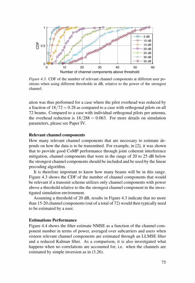
Number of channel components above threshold0 10 20 30 40 50 60

CDF

0

0.5

1

5 dB10 dB15 dB20 dB25 dB30 dB35 dB

Figure 4.3. CDF of the number of relevant channel components at different user po-sitions when using different thresholds in dB, relative to the power of the strongestchannel.

ation was thus performed for a case where the pilot overhead was reduced bya fraction of 18/72 = 0.28 as compared to a case with orthogonal pilots on all72 beams. Compared to a case with individual orthogonal pilots per antenna,the overhead reduction is 18/288 = 0.063. For more details on simulationparameters, please see Paper IV.

Relevant channel components

How many relevant channel components that are necessary to estimate de-pends on how the data is to be transmitted. For example, in [2], it was shownthat to provide good CoMP performance through joint coherent interferencemitigation, channel components that were in the range of 20 to 25 dB belowthe strongest channel components should be included and be used by the linearprecoding algorithm.

It is therefore important to know how many beams will be in this range.Figure 4.3 shows the CDF of the number of channel components that wouldbe relevant if a transmit scheme utilizes only channel components with powerabove a threshold relative to the the strongest channel component in the inves-tigated simulation environment.

Assuming a threshold of 20 dB, results in Figure 4.3 indicate that no morethan 15-20 channel components (out of a total of 72) would then typically needto be estimated by a user.

Estimations Performance

Figure 4.4 shows the filter estimate NMSE as a function of the channel com-ponent number in terms of power, averaged over subcarriers and users whensixteen relevant channel components are estimated through an LLMSE filterand a reduced Kalman filter. As a comparison, it is also investigated whathappens when no correlations are accounted for, i.e. when the channels areestimated by simple inversion as in (3.26).

75

In addition, results are shown where Kalman filters have been used assum-ing resources orthogonal pilots. In this set-up each channel component is thenassigned resource orthogonal pilots for all available subcarriers and for one outof 72 subsequent OFDM symbols. The total pilot power budget is the samefor the cases with resource orthogonal pilots as for the non-orthogonal pilots.Channel estimation by inversion by (3.26) is also performed for the orthogo-nal pilot case. In all case, the SNR per channel component is the inverse ofthe NMSE achieved by inversion with orthogonal pilots (the thin solid line inFigure 4.4).

While channel estimation by (3.26) may be sufficient for the strongest chan-nel components, it quickly degrades for weaker ones. Comparing channelestimation by (3.26) to the LLMSE filter, we see that by utilizing the spaceand frequency correlations, estimates are greatly improved, especially for theweaker channel components.

A further improvement of approximately 5 dB can be achieved by utilizingtemporal correlation by introducing the reduced Kalman filter.

The most effective approaches previously suggested for channel estima-tion for FDD massive MIMO is to optimize pilots for a specific set of users[74, 75, 76, 77]. To relate the presents results to those obtainable with pilotoptimization, we can compare the channel estimates based on non orthogonalpilots to those based on the orthogonal pilots when the reduced Kalman filteris used. In an extreme situation where the union of the sets of relevant chan-nel components of all the scheduled users includes no more than K (here 18)channel components, an optimization of pilots would result in the estimationperformance close to the one here obtained with orthogonal pilots 1. In a morerealistic situation, where the union of the sets of relevant channel componentsincreases with an increasing number of scheduled users, the estimation per-formance would move towards that of reduced Kalman estimation with nonorthogonal superposed pilots.

This reasoning indicates that the here proposed flexible solution, whichdoes not require pilots to be re-optimized every time a new user is scheduled,should in the worst case scenario result in a 5 dB reduction of the estimationNMSE performance, as compared to a case with optimized pilots for multipleusers. However, it should be stressed that a direct comparison with the pilotoptimization and channel estimation schemes of [74, 75, 76, 77] has not yetbeen performed.

There is potential to reduce the estimation error further, by estimating alsoadditional channel components that are below the threshold of relevance. Thisis illustrated by Figure 6 of Paper IV. It compares the estimation performance

1For a scenario of one of very few users, then it is likely that performance can be made muchbetter with optimized pilots as a result of optimizied power reallocation. With multiple usersand multiple base stations, it is unlikely that this will provide large gain. Reallocation can thenmainly remove power from beams that are of little value to any of the users. However, a similareffect can be achieved by using the beam deactivation scheme suggested in [69].

76

Channel component (sorted) k2 4 6 8 10 12 14 16

Aver

age

NMSE

[dB]

-30

-25

-20

-15

-10

-5

0

5

10

Inversion, non orht. pilotsInversion, orht. pilotsLLMSE, non orht. pilotsKalman, non orht. pilotsKalman, orht. pilots

Figure 4.4. Average NMSE sorted after the strength of the channel component.

2 4 6 8 10 12 14 16Number of channel components

6.8

7

7.2

7.4

7.6

7.8

8

8.2

8.4

Cpap

acity

[bits

/s/Hz

]

Kalman, orth. pilotsKalman, non orth. pilotsPerfect CSI

Figure 4.5. An illustration of the single user maximum ratio beamforming gain, basedon Shannon capacity, as a function of the included number of channel components.CSI is based on the two Kalman estimates in Figure 4.4. Note that the curves overlap.

77

of the reduced Kalman filter to that of a Kalman filter which estimates all 72channel components. These results indicate that a full order Kalman estima-tion performance with non orthogonal pilots becomes almost as good as thatgained by reduced-order Kalman filters with orthogonal pilots. However, asthe Kalman filter complexity grows with the square of the number of channelcomponents, the estimation of all channel components becomes highly com-putational complex. Therefore these results have only been evaluated for oneof the potential user positions, i.e. for only one potential set of relevant chan-nel components, and should hence be interpreted with care.

Paper IV also discusses potential methods of improving the reduced Kalmanfilter to attain a performance closer to that of the full-order filter without in-creasing complexity to unrealistic levels, e.g. by tracking the correlation prop-erties over time of the interference term Φ

τ , ¯relhτ , ¯rel in (3.25) through first orsecond order AR models. Such investigations are left for future work.

Capacity of MRC beamforming using estimated channels

The impact of the estimation errors in terms of MRC beamforming gain ishere illustrated in Figure 4.5. Maximum ratio beamforming to one user isperformed jointly by the nine base stations, by using a joint precoder, see Fig-ure 4.1. For each investigated user position, the precoder utilizes the estimatedchannels of the K strongest fixed beams for a particular user. Figure 4.5 showshow the resulting spectral efficiency increases with the number of K beamsthat are allowed to be utilized, on average over 100 user positions. The re-sults in this figure are assuming that the estimation performance is given bythe Kalman estimates presented in Figure 4.4. The Shannon capacity shownin the figure is for the single user case.

From Figure 4.4 we see that there is next to no beamforming gain fromhaving orthogonal pilots in this particular scenario. The reasons for this areas follows: First, the estimation quality is already very good for the strongestchannel components and an extra gain in accuracy will only translate into avery small capacity gain. Second, MRC beamforming gains are robust to es-timation errors. Third, as capacity grows logarithmically with SNR, addingextra channel component, that have low SNR as compared to the strongestchannel component, to the beam provides very little extra gain; note the satu-ration of the curves in Figure 4.5.

A separate study of interference supression by regularized zero forcing pre-coding in a CoMP cluster with massive MIMO antennas under a similar sim-ulation set-up as here, but with 288 beams, is presented in [69]. This studyalso includes a beam deactivation algorithm to ensure that no power would bewasted on beams that are weak to all users within the system. The results pre-sented there, with 10 % pilot overhead, show that performance loss, in terms ofpayload spectral efficiency, was approximately 12% compared to when perfectCSI was used.

78

4.2 Channel prediction for coordinated multipoint jointtransmission

In a traditional cellular network, each base station serves the users that are lo-cated within its own cell, see Figure 4.6. When a user moves from one cell toanother, the base stations cooperate in the hand-over procedure, but otherwisethey serve their users independently of each other. The base stations can usedifferent resources and/or different beams to avoid intracell interference, i.e.that the energy leaks between the different users’ messages. However, as basestations generally do not cooperate, except for in the hand-over procedure, en-ergy might leak between cells, causing intercell interference. This interferencedecreases the data throughput for the users and is especially severe for usersclose to the cell edges.

One option to decrease the intercell interference from nearby base stationsis to partition the available frequency spectra such that each base station onlyuses a fraction of the available spectrum. This method is called frequencyreuse. However, frequency reuse lowers the capacity of the system, as the basestations will only be able to serve it’s users with a fraction of the spectrum.

To increase spectral efficiency, present 4G systems allow all base stationsto utilize the whole available spectrum (this is called frequency reuse 1). Thedisadvantage of doing so is that the signals from several base stations will ingeneral be quite strong at the cell edges, thus causing intercell interference tobe the main limitation for users located at the edges.

A further way of increasing user throughput is to increase the spatial den-sity of base station and thus decrease the size of cells. If this is combinedwith frequency reuse 1, then intercell interference can become an even biggerproblem.

The intercell intereference can be limited by allowing a cluster of base sta-tions to cooperate to serve some or all of the users within their cluster of cells,using so called CoMP techniques. These were introduced in the beginning ofthe millennium as a way to increase the spectral efficiency of downlink trans-mission [57, 58, 79].

In a CoMP system, base stations share information over links that intercon-nect the base stations. These might e.g. be radio channels or fiberoptic cables.The base stations may be interconnected in different ways. The direct linksbetween two base stations are referred to as cross links. Links may connectbase stations to a CU which may be responsible for the joint transmission de-cisions. For future wireless networks, it is likely that many more base stationnodes will be deployed. With more nodes, operators may want these to be lessadvanced (and thereby less expensive), perhaps simply consisting of remoteradioheads. In such scenarios, a large part of the data and signal process-ing may be moved from the base stations into Radio Access Network (RAN)clouds that may include centralized baseband units. The links between radioaccess point and a centralized processing unit is in the literature often called

79

fronthaul link, if some or all of the RAN functionality is centralized [80]. Inthis section and in Paper II and Paper III, the name backhaul links will be usedfor all the connections in the fixed network side that are used to enable theCoMP processing.

Downlink CoMP is often divided into two categories, 1) JT and 2) JS and/orJB [81, 82, 83, 84]. In the first category, multiple base stations attempt totransmit to one, or more, users simultaneously, see Figure 4.7, while in thesecond category, base stations coordinate their transmission, e.g. such thatthey avoid serving closely located users within the same resources and therebylower the intercell interference. In JT we try to utilize the potentially stronglyinterfering links from neighbouring base stations, turning a potantial probleminto an advantage. With JS and JB, we mainly strive to avoid interference. Forthis reason, JS and JB provide lower gains in spectral efficiency than JT, butare more robust to errors in CSI [3, 85].

In CoMP JT, base stations share both payload data and CSI over the back-haul links. Based on the CSI, some or all of the base stations may then beselected to transmit payload to one user, without any pre-compensation of themessage symbol intended for that user. As the message is transmitted with ra-dio waves these may sometimes add up constructively at the users, providing astronger receive signal than if only one of the base stations transmitted. How-ever, when no pre-compensation of the message is used, then the signals mayalso add up destructively, lowering the total received power2. This is callednon coherent CoMP JT.

An alternative is that the base stations precode the message symbol, basedon the CSI, before transmission, to ensure that the signals from the differentbase stations add up constructively. This scheme, which is called coherentCoMP JT or network MIMO, allows base stations to serve multiple users onthe same time-and-frequency slot, or resource. The messages are then pre-coded such that, at each user, only the message intended for that user is con-structively added, while the messages intended for the other users are addeddestructively.

The results in this section are extracted from Papers II and III. They aim toinvestigate

1. How well channels can be predicted. A challenge with downlink CoMPare the long system delays. These include the processing time for chan-nel estimation, the feedback of measurement or CSI feedback from theusers to the base stations in FDD systems, the CSI sharing between thebase stations over backhaul, the process time for the precoder designand the sharing of the precoder weights between base stations or be-tween a centralized unit and radio access points over fronthaul links in acloud RAN architecture. The sum of these system delays can be in theorder of of tens of milliseconds, which for mobile users will cause the

2On average the received power will be stronger.

80

����

Figure 4.6. A set-up of a cellular network where each base station (BS) serves theusers in its own cell only. Different colors indicate messages intended for differentusers. In the absence of base station cooperation, some of the energy intended for auser in one cell might leak to a user in another cell, causing interference.

����

Figure 4.7. A set-up of a CoMP JT scenario where three base stations (BS) transmitjointly to three users. The base stations share information over backhaul links via acontrol unit (CU).

81

CSI to be outdated at the time of transmission [86, 87, 88]. The outdat-ing of CSI can to some extent be counteracted by channel predictions[33, 1, 89, 38]. Here, Kalman predictions are investigated for differentprediction horizons based on channel measurements.

2. How the performance of coherent CoMP JT is affected if knowledgeof the prediction performance (in terms of second order statistics of theprediction errors) is accounted for in the precoding step as comparedto when this is not the case. The investigated precoder, which aims tomaximize the sumrate, uses not only the Kalman predictions for pedes-trian users, but also the knowledge (through error covariance matrices)of their accuracy. It is compared to a precoder that only utilizes thechannel predictions.

3. How to deal with different backhaul constraints. Such limitations mustbe handled by the precoder.

4. How to improve performance by a simple user grouping and resourceallocation scheme. Some of the large gains from MIMO techniques arerelated to serving multiple users simultaneously. However not all usersare spatially compatible and a technique for grouping users is required.The proposed scheme assumes that each base station schedules the userswithin its own cell independently using channel aware scheduling. Theusers scheduled on a specific resource are then served by CoMP JT.

4.2.1 Background and related workCoherent CoMP JT has the potential to provide very large gains in spectralefficiency (see e.g. [59, 82, 90, 91, 92, 87]), gains that are especially importantfor cell edge users [93, 81, 2, 94].

CoMP can also be applied for uplink transmission, either through JS orthrough joint detection, see e.g. [94, 95]. Joint detection in the uplink issimilar to JT in the downlink. However, it is an easier problem in the sensethat the processing can be based on fully updated CSI.

The cooperation cluster

There is a trade-off in the number of base stations included in the cooperationcluster. In a cluster with a low number of base stations, the remaining uncom-pensated intercluster interference will be large, lowering the potential CoMPgains. In a cluster with a large number of base stations, there might be largesystem delays, causing severe outdating of the CSI. This, in turn lowers poten-tial CoMP gains. Moreover, in very large clusters, base stations will be so faraway from each other that this may cause severe synchronization problems.

The problem of clustering has been studied for intracluster interference lim-ited scenarios in e.g. [92, 96, 97, 98]. According to these works, for singleantenna base stations, clusters of about three base stations are sufficient in or-der to achieve most of the CoMP gains. After this point, CoMP gains grow

82

Figure 4.8. Centralized coordination of downlinks in an FDD system. A schematic fig-ure of data transmission of feedback over wireless uplinks (gray arrows) and backhaullinks (black arrows). Dashed arrows indicates coherent joint downlink transmissionof the payload data.

slowly. For MIMO systems with 2-4 transmit antennas per base station, clus-ters of 7-9 base stations are required.

Such cluster sizes are fairly small, so intercluster interference levels willstill be significant. Therefore external schemes to manage intercluster inter-ference can improve the CoMP gains further. An interesting method to limitthe intercluster interference is proposed in [96] and further evaluated in [99].It uses cluster-specific antenna tilting and power control for this purpose.

Network architecture

A CoMP network may be centralized, distributed or semi-distributed. In adistributed network, each base station forwards CSI to other base stations andthen designs a precoder separately. Then, base stations will in general haveaccess to different information, and hence the set of precoders differs fromthat of a centralized design3. In centralized CoMP, all CSI is transmitted toa CU, where the precoder is designed, and all base stations are provided withtheir relevant scheduling decisions, beamforming weights and payload data.

The CoMP JT system considered in this thesis assumes a centralized archi-tecture as illustrated in Figure 4.7, unless otherwise specified.

For downlink coherent JT in a centralized CoMP architecture, CSI needs tobe obtained for all users at their master base stations, i.e. the base station that isthe strongest, seen from the user’s perspective. These then need to share boththe CSI, and the payload data amongst each other over a backhaul network. ACU, which is a logical entity that may be located at one or more of the basestations within the cooperation cluster, then calculates the precoder. Finally,the elements of the precoder matrix are, if necessary, transmitted to the basestations, see Figure 4.8.

A disadvantage of a centralized scheme is that the system delays will belonger as information needs to be transmitted over backhaul/fronthaul linkstwice. Delays in the fixed network causes outdated CSI, which can severely

3For example, if the users feed back CSI to their main base station at frequent intervals, theneach base station may have access to less outdated CSI from the users within its own cell thanit has to the users within its neighbouring cells.

83

reduce gains [86, 100, 21]. In order to compensate for the system delays,channel prediction is necessary.

For more information on the different architectures, see [21, 22].

Precoding

The highest gains for coherent CoMP JT are achieved with Dirty Paper Coding(DPC), see e.g. [101]. However, as this non-linear precoding scheme is highin complexity, linear precoding is an important topic of investigations. Theprimary objective of the precoder is often to limit the intracluster interference.In a system with perfect CSI this can be achieved by channel matrix inversion,which is provided by the zero forcing precoder developed for MIMO, see e.g.[25].

However, there is a risk in using zero forcing for CoMP JT , even in the pres-ence of perfect CSI; Channel gains may from different base stations be verydifferent in amplitude, which is generally not the case for MIMO downlinkwhere all transmit antennas are co-located. The balancing of transmission sig-nal gains that is necessary for channel inversion might then cause the strongestbase station’s transmit power to become very low as compared with the weak-est base station. Although the solution is then still optimal with respect tolimiting intracluster interference, the noise and intercluster interference mightbecome large compared to the received signal power, resulting in a poor datarate. An option is then to use an MSE criterion which takes these effects intoaccount as well as the intracluster interference [26].

MSE criteria are attractive as they generally have analytical solutions. How-ever, in practice it is often more useful to optimize over a weighted sumratecriterion, as this is closer to the desired end performance. Such an optimiza-tion poses a multidimensional nonconvex optimisation problem.

In the precoder design proposed in Paper II, which is an extension of thedesing introduced in [4], a heuristic solution is used, which strives to maxi-mize an approximation of the sumrate by iteratively adjusting a set of parame-ters, that are criterion weights in a (robust) MSE criterion. The MSE problemstated is derived from a robust linear-quadratic optimal feedforward controlframework developed by Öhrn, Ahlen and Sternad in [102]. This general so-lution is also used for e.g. audio processing, see e.g. [103].

A problem with CoMP JT in a centralized network is, as previously men-tioned, that the long delays cause inaccuracies in the CSI. If these inaccuraciesare not addressed in the precoder design, then the potential CoMP gains maybe lost. Robust precoder design techniques have been suggested for Mul-tiple-Input Single-Output (MISO) systems by [104, 105], and for multi-userMIMO downlinks in [106, 107]. A robust linear precoder for CoMP JT, whichis based on an MSE criterion, is suggested in [108].

In comparative studies in [2] and [109], the design discussed here was com-pared to designs suggested in [108] and to an optimization approach proposedin [110]. It was shown that the here suggested design performed better than

84

the robust precoder suggested by [108] and close to that of [110], at a muchlower computational complexity than the latter.

How to handle limited backhaul

The requirements on backhaul might not always be manageable by the system.Structural constraints, delay constraints, capacity constraints or a combinationof these might limit the information that can be transmitted over backhaul.These limitations must be handled by the precoder. In the formulation sug-gested here, this is achieved by setting some elements in the precoder matrixto zero. These elements represent the input-output connections that are un-available. Such zeros can be forced into the precoder matrix in different ways.

One option to force zeros into the precoder when backhaul constraints arepresent is to simply calculate the precoder, based on some criterion, and thenset the required elements to zero, see e.g. [111]. However, the resulting pre-coder is then no longer optimal with respect to the criterion it was optimizedfor. Another option is to only feed back the channels that are going to be uti-lized in the transmission and then group users such that the channel matrixbecoms block diagonal. Then, through channel inversion, the resulting pre-coder will automatically have zeros in the required elements [112]. However,such a solution requires JS and may therefore potentially add large demandson backhaul capacity in the user grouping step. Furthermore, the suggestedmethods in [111, 112] do not consider the inaccuracy of the CSI in the precod-ing design.

A strength of the here proposed precoder is that the MSE criterion (withtuning of criterion weights to approximate a weighted sumrate solution) canbe used also under backhaul constraints. This can be done by introducing largepenalty terms in the robust MSE criterion. This modification only requires alow number of extra calculations and is therefore of much lower complex-ity than methods that use multidimensional searches to optimize the nonzeroelements of the precoder, see e.g. [110, 113, 114].

In [115] a different method for forming sparse precoders matrices to fulfilbackhaul constraints is suggested. This precoder, which is based on an MSEcriterion that includes intracluster interference only, is also low in complexity.However, as the matrix dimensions do not add up in the published design equa-tions of this paper and its simulations are based on very few user positions, itis hard to draw any conclusions from the paper. Moreover, this method doesnot have the flexibility to optimize over arbitrary criteria, nor does it considerCSI errors in the design.

User grouping and scheduling

A way of determining which users should be jointly served by a CoMP clusteris to form groups based on spatial compatibility, without considering the inde-pendent small scale fading of the channels to the users, as in e.g. [111, 116]. Ina second step the user groups are then allocated resources. There is a large risk

85

Figure 4.9. System model used for precoder design.

with this type of scheme; the users generally have uncorrelated fading, so oneor more of the users in the group may have a poor channel for the particularresource allocated to the group.

The problem with the small scale fading of different users can be solved byjointly performing user grouping and scheduling. However, the combinatorialgrowth of the complexity associated with finding the best set of users to begrouped into each time-frequency transmission resource makes it infeasible, ifthe number of transmission resources and users is large. In order to decreasethe number of combinations, a greedy user grouping and scheduling algorithmcan be used. This has been suggested for downlink single cell MIMO trans-mission in e.g. [117, 118] and for uplink CoMP in [119].

A user grouping and scheduling algorithm similar to that which will be pre-sented and investigated here can be found in [120], where instead of focusingon increasing rate it is focused on increasing rate dependent utility functions,for the different types of packet streams.

4.2.2 Robust linear precoding design and user groupingThe robust precoder that was introduced in [4] and further developed in PaperII is designed based on the system model shown in Figure 4.9. Here, a vectorof complex valued symbols s ∈ C

M×1 to M single antenna users is projected,through a precoding matrix R ∈ C

N×M, onto N signals, collected in the vectoru ∈ C

N×1, that are to be transmitted from N different antennas. The transmitsignals are scaled to ensure that power constraints are met through a real val-ued scalar 1/c. This describes the downlink transmission over one narrowbandsubcarrier in an OFDM system.

The transmit signals are thus assumed to propagate over linear narrowbandchannels. Furthermore, Gaussian noise is assumed to be added at the receiver.This can be mathematically modelled by

y = Hu+n, (4.3)

86

where y ∈ CM×1 is the vector of received message symbols at the users andn∈C

M×1 is the noise and intercluster interference added at each users’ receiveantenna. The matrix H ∈ C

M×N is the channel matrix containing the complexvalued channel elements between each user and the transmit antennas at thebase stations. It consists of a sum of a known prediction H and predictionerrors ΔH.

A second system is considered. In this a target vector z ∈ CM×1 of the

desired interference free scaled received symbols is defined by

z =1c

Ds, (4.4)

where D ∈ RM×M is a diagonal weighting matrix, that ensures that we do notask more of the system than it is able to carry out. For examples, if all basestations have weak signals to a user, then the diagonal element of that usershould be set small, e.g. scaled to the channel gain from nearest base station.

The precoding matrix R is designed to minimize a scalar weighted robustMSE criterion

J = E[E ‖Vε‖ 2 +E ‖Su‖2] . (4.5)

Here E denotes the expected value with respect to the prediction errors (theelements of ΔH) while E denotes the expected value over the involved signals.The weighting matrices V and S are design parameters that can be adjustedso that the solution R that minimizes (4.5) will approximate the solution thatoptimizes a different objective function, see Paper II for details. In the evalua-tions presented below, V = I and S is chosen diagonal, with diagonal elementsadjusted to maximize an approximation of the sumrate.

Assuming that all message symbols are mutually uncorrelated and also un-correlated over time, with unit power, the linear precoder that minimizes (4.5)is given by

R =(H∗V∗VH+S∗S+E[ΔH∗V∗VΔH]

)−1H∗V∗VD. (4.6)

The accuracy of the channel predictions are accounted for in the third termof the inverse. For details on how to calculate this term or how to derive theexpression (4.6) the reader is referred to Paper II and Paper III.

In the experimental evaluation of Paper II, the sumrate performance whenusing (4.6) is compared to that obtained when using a zero forcing precoder

R = HT(HHT

)−1D. (4.7)

It is important to include the diagonal target scaling matrix D as a right factoralso of the zero forcing precoder (4.7). The sumrate performance is impairedotherwise, due to power scaling issues, in particular in fully loaded cases whenM = N.

87

Before a precoder can be designed, the system needs to determine whichusers to serve on the individual transmission resources. On each resource,M ≤ N users can be grouped for JT.

From results in [4], it was clear that the performance of coherent CoMPJT in a fully loaded system M = N (i.e. when the number of served userswithin a resource, matched that of the number of serving antennas at all basestations) was worst when all users had weak channels to the same base station.The conclusions that such users are spatially incompatible is intuitive, as theweak base station cannot offer much support in the transmission and hence thesystem is in practice overloaded. Based on this, the user grouping method pro-posed in Paper II, which is denoted cellular user grouping, focuses on makingsure the that different users who share a resource will have different strongestbase stations. This will make the channel matrix H diagonal dominant forsingle-antenna base station, if users are numbered appropriately. It will thusbe made more easily invertible.

This aim could be attained in various ways. The here proposed methodutilize an assumption that the system has cellular structure and that separatescheduling is performed for users that are assigned to each cell, performingchannel aware scheduling. As a pleasant suprise, it turns out that by utilizingthe results of these separate scheduling decisions, good user groups are formedspontaneously for the cluster of cells.

In this scheme, each base station schedules all users within its own cellonly. The scheduling may be based on some coarse CQI of these users, e.g.a roughly quantized, resource specific, estimate of the of the channel powergain. The scheduler is assumed not to allocate a user to transmission resourcesin which it has an unusual weak channel. As a consequence, the scheduledusers will have a reasonably strong channel to its own base station within eachof the time-frequency resources it is assigned to use. Then, groups are formedfor each time-frequency resource as the users that have been assigned to thatresource by all the separate cellular schedulers within the cooperation cluster.As a result, users that will be jointly served on a resource will then likely havedifferent strongest base stations, namely their own base stations 4. The schemehas the advantage that it only needs a CQI to allocate resources and therebyforming the user groups. This lowers the feedback overhead that is needed ascompared to e.g. a user grouping scheme that uses the complex valued channelgains to all users in all cells to find the optimal user groups.

4When one user has equally or almost equally strong channels (on average) to more than onebase station, it will still have to be assigned to one of these. That base station will then be incharge of scheduling the users without any knowledge of the small scale fading of the channelsbetween the user and the other base stations. It may therefore occur that the user has equallystrong or stronger channel to a different base station for the resources that it will have beenassigned. This should however not pose a problem, as the user then has two strong channelcomponents.

88

The cellular user grouping may, but does not have to, utilize already exist-ing scheduling algorithms. For example, if the objective is to maximize thesumrate, then the base station might schedule the user that has the best CQIfor any given resource. If fairness amongst users is considered, then a pro-portional fair scheduler, which allocates the resource to the user that has thehighest ratio of its CQI for the given resource relative to its average CQI forall resources, see [121], can be chosen. Another option, which will be used inthe results below, is to use the score based scheduler introduced in [122].

In the evaluation in Paper II, each cell has one base station antenna andschedules at most one user in a resource. This can be generalized to multiuserMIMO transmission within cells. It need then be assumed that the mutualspatial compatibility of users that are scheduled on the same resource within acell is taken care of by each cellular (multiuser MIMO) scheduler. These usergroups are then merge into user groups for the whole cooperation cluster.

Simulation results

The proposed channel predictions, precoding design and user grouping schemehas been evaluated based on channel sounding measurements that were col-lected in Kista, in Sweden, by Ericsson Research in December 2008. In these,channel sounding pilots were transmitted in a 20 MHz band, at a carrier fre-quency of 2.66 GHz from three omnidirectional single antenna base stationslocated in an urban environment, see Figure 4.10.

The pilots were measured by a vehicle which was driving through the areabetween the base stations. The powers of the signals received from the dif-ferent base stations are presented as a function of the measurement locationin Figure 4.11 and as a function of time in Figure 4.12. The time series wereresampled so that the true maximal vehicle velocity corresponded to a veloc-ity of 5 km/h in the resampled time series. The quality of the measurementsare very high and in the simulations included in the papers, the correspondingestimates of the OFDM channels are regarded to be the exact channels. Moredetails on the set-up for this measurement campaign can be found in Paper IIand in [123].

Based on these channel measurements, pilot measurements with differentpilot SNRs were simulated for each user position plotted in Figure 4.12. Thesemeasurements were simulated through (3.2) using resource orthogonal pilotsand Gaussian noise. Then, the channels were predicted for prediction horizonsthat correspond to distances of {0,0.6,0.13,0.19,0.28} of the carrier wave-length in space, corresponding to system delays of {0,5,10,15,23} ms at auser velocity of 5 km/h. The resulting NMSE was averaged over a time of 0.5s for each user position and a total of 144 subcarriers5.

5Further simulation assumptions are described in Paper II.

89

Figure 4.10. The urban environment of Kista, Stockholm, seen from above. Thelocations of the base stations (BS) are marked by triangles.

17.568 17.57259.242

59.244

59.246

Longitude

Latitu

de

17.568 17.572Longitude

17.568 17.572Longitude

−120

−100

−80

Figure 4.11. The signal powers in dBm from base station 1 (left), base station 2(middle) and base station 3 (right). The base station locations are marked by triangles.

0 5 10 15 20−120

−100

−80

Time [min] (at maximum speed 10 km/h)

Powe

r [dB

m]

Figure 4.12. The variations of the power of the received signals that were transmittedfrom base station 1 (blue), base station 2 (green) and base station 3 (red). For details,see Paper II.

90

Figure 4.13 shows the prediction performance, in terms of average NMSE.The results are compared to the NMSE that would result from using outdatedCSI, i.e. using the channel estimate hτ as a prediction for the channel hτ+m.

We see that while the outdated CSI very quickly decrease in accuracy, withan increasing prediction horizon, predictions through the Kalman filter providean average NMSE ≤ −7.9 dB for prediction horizons of up to 0.28 of thecarrier wavelength. As these predictions are based on real measurements andestimated channel models, that is very encouraging. It is worth noting that,as stated in Section 3.4, the measurement noise has lower impact for longerprediction horizons.

As promising the results in Figure 4.13 are, they do not show the full statis-tics. In Figure 4.14 the CDFs of the prediction NMSE are shown. Althoughmost of the channels are predicted with good accuracy, there are some poorpredictions among the weaker channels. For example, with the highest noisefloor at −110 dB more than 30% of the channels have an NMSE of −8 dBor higher if a prediction horizon of 0.13 of the carrier wavelength is required.For the longest prediction horizon (0.28 of the carrier wavelength) this fractionincreases to approximately 50%.

From Figure 4.12 it is evident that it is often the case that the signals fromone or two of the base stations are much weaker that the strongest base station.Inaccurate predictions for weak channels may not be a big problem if these arevery weak compared to the strong channels, as they would not contribute muchto the beamforming gain.

However, it is important that these weak channels with inaccurate chan-nel estimates do not deteriorate the quality of the total precoding solutions.This can potentially be avoided if information of the prediction accuracy isaccounted for when designing the precoder.

Figure 4.15 shows the performance in terms of sumrate when the three sin-gle antenna base stations serve a group of up to three users on each of the 144subcarriers, using joint coherent precoding. These are the sumrates that wereachieved when nine users were randomly picked from the possible positionsalong the driving route shown in Figure 4.11 and were served jointly by thethree base stations within the 144 subcarriers. The investigated scenario is a(small) fully loaded case, where the three single antenna base stations servethree users in each transmission resource, so M = N = 3.

First, we will focus on the solid curves of Figure 4.15. Here, the nine userswere randomly assigned into group of three users, that were then randomly as-signed to each subcarrier. The users were then served through coherent CoMPJT either by zero forcing precoding (circles) or though the robust linear pre-coder (4.6) (squares) when the precoding matrix is based on the predictedchannels with a prediction horizon of 0.13 of the carrier wavelength. Thecriterion weight S in (4.5) is diagonal, and is adjusted to maximize an approx-imation of the sumrate. As a comparison, the sumrate that would be achievedby using zero forcing with perfect CSI is also added (diamonds).

91

0 0.05 0.1 0.15 0.2 0.25 0.3Prediction horizon [ ]

-30

-25

-20

-15

-10

-5

Aver

age

NMSE

[dB]

Figure 4.13. The solid lines show the prediction performance in terms of averageNMSE for all base stations, user positions and subcarriers as a function of the predic-tion horizon scaled by the carrier wavelenght λ . Results are shown for noise levelsof −110 dBm (crosses) −120 dBm (pluses) and −130 dBm (stars), see Figure 4.12.Dashed lines show the NMSE of the outdated CSI. Further details can be found inPaper II.

-40 -35 -30 -25 -20 -15 -10 -5 0NMSE [dB]

0

0.2

0.4

0.6

0.8

1

CDF

Different noise floors

Figure 4.14. CDF of the prediction NMSE for different measurement noise levels−110 dBm (crosses) −120 dBm (pluses) and −130 dBm (stars). Prediction horizonsof 0 carrier wavelengths (black dotted lines), 0.13 carrier wavelengths (purple solidlines) and 0.28 carrier wavelengths (blue dashed lines). For further details, see PaperII.

92

We can see, by comparing zero forcing with robust linear precoding, thatknowledge about the prediction accuracy is important in this situation, espe-cially when we compare the low percentiles in the CDFs at high noise floor(-110 dBm). Here, the sumrate is increased significantly. The gap is low-ered as the noise level decreases. However at no point does the robust linearprecoder provide a worse sumrate than zero forcing.

Now consider instead the dotted curves, representing results for the nineusers that are grouped by cellular scheduling with score based schedulers.That is, for each simulation, the users that have the same strongest base stationare assumed to belong to the same cell and are therefore scheduled on differ-

ent subcarriers using the score based scheduler introduced in [122]. Usersscheduled on the same resource are then served jointly by the base stations.

This simple user grouping scheme has the effect that the problem withbad user grouping becomes insignificant. Comparing the dotted and the solidcurves, the large impact of using a reasonable user grouping scheme becomesevident. First, and most striking, there is a large improvement in sumrate per-formance. Second, the impact of different precoding schemes is altered. Atthe lowest noise floor (−130 dBm), zero forcing now even outperforms robustlinear precoding. At first, this may seem suspicious, however it is a case of be-ing overly confident in the information we have. Recall from Section 3.4 thatthe channel model is estimated from imperfect training data. That means thatthe information we have in regards to the accuracy of the channel prediction isslightly off. For most theoretical scenarios, this is not an issue as the estimatedaccuracy is not far from that of the actual accuracy, see e.g. Chapter 8 of [1]where this was investigated for the channel data set used here. However, as thesystem is pushed to the bounds, as in this case with very low noise floor andvery good user groups, the errors made in estimating the prediction accuracywill cause the robust linear precoder to actually perform somewhat worse thanzero forcing.

In addition to the results presented here, Paper II provides simulation resultswhere the proposed cellular user grouping method presented here is comparedto a high complexity, greedy user grouping scheme, which iteratively adds ausers to the group within each resource. The simulations, which are basedon block fading channels, show very little performance loss with cellular usergrouping as compared to the greedy user grouping scheme.

4.2.3 Handling backhaul limitationsDepending on the infrastructure, the requirements on the backhaul might notalways be manageable, and hence we need a method for handling constraintson how much information that can be sent over the backhaul links.

Limitations in how much CSI can be fed to the CU can be handled by settingthe unavailable channel estimates to zero and adjusting the covariance matrices

93

0 5 10 15 20 25 30 35 40 45 50Sumrate [bps/Hz]

0

0.2

0.4

0.6

0.8

1

CDF

0 5 10 15 20 25 30 35 40 45 50Sumrate [bps/Hz]

0

0.2

0.4

0.6

0.8

1

CDF

0 5 10 15 20 25 30 35 40 45 50Sumrate [bps/Hz]

0

0.2

0.4

0.6

0.8

1

CDF

Figure 4.15. CDFs of the sumrate for all user groups when nine users are randomlydropped along the route shown in Figure 4.11 and grouped over 144 subcarrier withup three users to be jointly served per subcarrier. Results are shown when the precod-ing matrix is obtained through zero forcing precoding (circles) or through the robustlinear precoder (4.6) (squares). Users are either grouped randomly and then allocatedresources randomly, by so called round robin scheduling, (solid lines), or by cellularuser grouping, when each of three cells allocates its users using a score based sched-uler (dotted lines). Results for noise floors of −110 dBm (top), −120 dBm (middle)and −130 dBm (bottom). Results with perfect interference suppression by zero forc-ing with perfect CSI (diamonds) is added for comparison. For further details, seePaper II.

94

of the error accordingly, see Paper III for details. As the error covariancematrices only need to be sent on a slow time scale, e.g. every half second,these place very low demands on the backhaul capacity.

However, we may also need to limit the number of non-zero elements in theprecoding matrices that are distributed to the base stations.

Furthermore, assume that the sharing of payload data between sites is lim-ited so that only some of the payload can be shared. Then, some base stationswill not have access to all the symbols of the data vector s. This can be math-ematically modelled the same way as when a limited number of precodingweights can be fed back to the base stations from the CU, i.e. by setting theappropriate elements of the precoding matrix R to zero. That is, if no datais available at base station antenna n for user m, then element {n,m} of theprecoding matrix, rn,m, should be set to zero.

In Paper III, this is done by extending the criterion (4.5) to

J = E

[E ‖V ε‖ 2 +E ‖Su‖2 +E

N

∑n=1

M

∑m=1

1c2 |wnmrnmsm|

2

], (4.8)

where sm is the message symbol for the m’th user and the scalar wnm is apenalty weight that is set high if the element rnm of the precoder matrix R

needs to be zero and is set to zero otherwise.The solution which minimizes this criterion is found by first calculating the

precoder that minimizes the original criterion, which is given by

R0 = (β ∗β )−1H∗

CU V∗VD, (4.9)

where HCU is the available estimate of the channel matrix at the CU and

β ∗β = H∗CU V∗VHCU +S∗S+E[ΔH∗

CU V∗VΔHCU ]. (4.10)

Then the precoder with (approximately) enforced zeros is given by solving alinear matrix equation

R = R0 − (β ∗β )−1 (WWR) . (4.11)

Here W is the matrix given by the weights wnm and denotes elementwisemultiplication.

Results in Paper III are based on a simple simulation environment with threesites, each with three sectored base stations with two antennas each and ninerandomly distributed single antenna users with at most one allocated user percell and transmission resource. A large number of sets of user positions issimulated. The channels are modelled as block fading and channel errors aremodelled as complexed-valued zero mean Gaussian variables with a variancewhich is 20 dB below the channel variance. No shadow fading is considered.The results in Paper III show that there is a gain in the average user rate of upto 13% when using the proposed precoder with the extended MSE criterion,

95

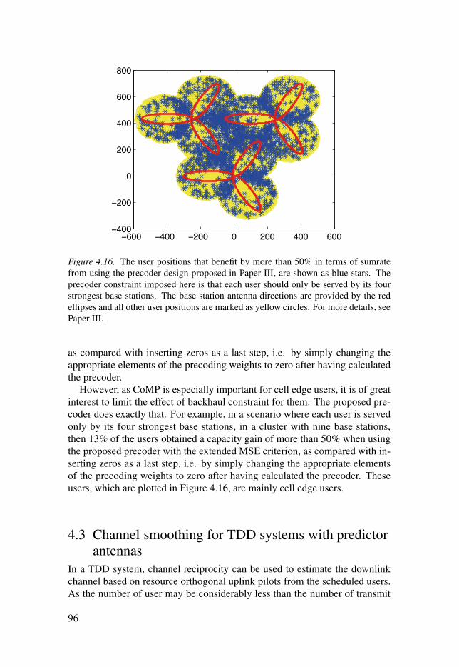
−600 −400 −200 0 200 400 600−400

−200

0

200

400

600

800

Figure 4.16. The user positions that benefit by more than 50% in terms of sumratefrom using the precoder design proposed in Paper III, are shown as blue stars. Theprecoder constraint imposed here is that each user should only be served by its fourstrongest base stations. The base station antenna directions are provided by the redellipses and all other user positions are marked as yellow circles. For more details, seePaper III.

as compared with inserting zeros as a last step, i.e. by simply changing theappropriate elements of the precoding weights to zero after having calculatedthe precoder.

However, as CoMP is especially important for cell edge users, it is of greatinterest to limit the effect of backhaul constraint for them. The proposed pre-coder does exactly that. For example, in a scenario where each user is servedonly by its four strongest base stations, in a cluster with nine base stations,then 13% of the users obtained a capacity gain of more than 50% when usingthe proposed precoder with the extended MSE criterion, as compared with in-serting zeros as a last step, i.e. by simply changing the appropriate elementsof the precoding weights to zero after having calculated the precoder. Theseusers, which are plotted in Figure 4.16, are mainly cell edge users.

4.3 Channel smoothing for TDD systems with predictorantennas

In a TDD system, channel reciprocity can be used to estimate the downlinkchannel based on resource orthogonal uplink pilots from the scheduled users.As the number of user may be considerably less than the number of transmit

96

antennas for massive MIMO systems, the pilot overhead may be considerablysmaller than in an FDD system even if resource orthogonal pilots are used.

With wireless access playing a more and more important role in peoplesdaily life, problems may occur when many users are a gathered in the samesmall location, creating so called hot-spots. A typical hot spot scenario occurswithin the sector of public transportation such as trams or buses where peopleuse their mobile wireless communication equipment both for work and forentertainment purposes [124].

While linear prediction works well for pedestrian users, it may not be suffi-cient for high mobility users when the delays between the pilots and the datatransmission are of significant duration. An example is a TDD system wherethe user equipment would transmit known pilots during an uplink frame, thatare used for channel estimation on the network side. Assuming channel reci-procity, these channel estimates are then used to calculate predictions of thechannels to the user equipment antennas during a subsequent downlink sub-frame. The required prediction horizon for the downlink channels could thenbe on the order of the magnitude of the carrier wavelength in space, for vehic-ular users.

An approach to increase the prediction horizon might be to have a databaseof pre-recorded coordinate specific CSI, e.g. located at the base stations [125].The users can then feed back an estimate of their locations, e.g. based onGlobal Positioning System (GPS) information, to the base stations. As thismethod would not really be predicting the fading in the conventional sense,it is not bound by the limitations discussed in Section 3.4. However, such amodel would require collection of a vast amount of data on centimetre scalein space. This data might in turn need to be updated continuously, due to e.g.seasonal changes in the environment. It is also unclear how such a schememight be affected by e.g. bypassing vehicles that alter the standing wave pat-tern. It is therefore of interest to investigate more easily realizable long-rangechannel prediction methods for vehicular users.

4.3.1 History of the predictor antenna conceptThe limit of prediction horizon can be circumvented by the predictor antennaconcept which is illustrated in Figure 1.4. It uses an extra antenna, predictorantenna, placed in front of one or several main antennas, e.g. on the roof ofthe vehicle, to scout the channel that will later be encountered by the mainantennas. This concept was originally proposed by Sternad et al. in [27],where the potential of predictor antennas were illustrated based on a smallmeasurement campaign with one LOS and one NLOS scenario, using twodipole antennas on the roof of the vehicle.

A second measurement campaign with monopole antennas and a large metalsheet under the antennas showed improved results [43, 126, 127]. Further ex-

97

perimental studies, conducted by Björsell, Sternad and Grieger have showna prediction NMSE of about -10 dB for vehicular velocities for all measuredpredictions horizons up to three times the carrier wavelenght in space, tentimes longer than the limit for channel extrapolation [128, 129]. The methodhas recently been applied to 64-antenna massive MIMO downlinks, and wasshown to provide close to ideal maximum ratio transmit beamforming gainsto vehicles over NLOS channels [130].

To produce accurate predictions, the concept requires channel estimates forthe predictor antenna from positions close to where the main antenna willtransmit or receive signals. For a FDD system, this requires dense enoughdownlink channel estimates, which was the case in [128, 129, 130], whereOFDM pilots, evenly distributed in time and frequency, were used.

Similar antenna systems as in [27] with two in-line antennas on a vehi-cle roof, were investigated in the 90’s by Vaughan and coworkers [131, 132].The aim was there not prediction, but to model the radio environment. Theseexperimental results showed that the maximal cross correlation between thesignal envelope at the rearward antenna and the delayed signal envelope at theforward antenna was reduced when the antennas were separated by 0.2-0.4times the carrier wavelength, due to antenna coupling. In [132], the effectsof the antenna coupling were compensated for a to a large extent. Similar re-sults were found in [43, 126, 127] and the antenna coupling was sucessfullycompensated for in [127].

4.3.2 Kalman smoothing for TDD downlink estimatesEven when using predictor antennas, the distance between the antennas maynot be perfectly aligned with the required prediction horizon (as this will de-pend on the users speed). For a TDD system, the uplink/downlink ratio to theTDD frame might be adjusted so that the downlink transmission of the mainantenna occurs close to a position where the predictor antenna already hasmeasured the channel, as proposed in [28] and evaluated in [133]. However,such a scheme would require individually adaptable uplink/downlink ratiosbased on the velocity of each user which is problematic from a system per-spective. Instead, as suggested in [133], interpolation can be used for anygiven uplink/downlink ratio to generate channel estimates for the gaps in theuplink pilot sequence.

The results of Paper V, which are highlighted in this section utilize Kalmansmoothing to interpolate the channels during TDD downlink frames, by usingreceived uplink pilot signals from the predictor antenna in uplink frames. Theinterpolations use a two-filter approach, using two state space models.

The Kalman smoother is the MMSE-optimal linear interpolator of noisydata, for known second order statistics of signal and noise [10]. It has beenstudied in applications such as the compensation for packet loss in wireless

98

sensor network system [134] and for channel equalization on the receiver side[135], in both cases where partial observation losses occur.

To gain understanding of the concept, let us consider a predictor antennasystem with two antennas, spaced by a fixed distance and placed in a straightline in the direction of travel on a vehicle, as was illustrated in Figure 1.4. Wedefine a time interval indexed by τ , which shall here be denoted time slot andwhich represents the time between potentially pilot bearing OFDM symbols.(Between these OFDM symbols separated by τ , data bearing OFDM symbolsare in general be transmitted.)

Assume that required prediction horizon is m time slots and assume thatthe vehicle is travelling with a velocity such that it takes m+ μ time slots forthe main antenna to reach the position of the predictor antenna. As the mainantenna will experience approximately the same channel as the predictor an-tenna, with a time lag of m+μ time slots, the prediction of the main antenna’schannel at time τ +m can be given as a smoothed estimate of the predictorantenna’s channel at time τ − μ . We can therefore use up to μ later channelestimates to improve the estimate of the channels from the predictor antennaat time τ , if measurements are available at these later time slots.

An example of this is illustrated in Figure 4.17, where a channel from onebase station antenna in a TDD system is to be estimated. Here, pilots are trans-mitted in the uplink for three consecutive pilot slots, indexed by τ , followed bya downlink with three consecutive slots of equal length to the uplink slots butwithout pilots. In this example it is assumed that m= μ = 5 time slots and thatthe vehicle is travelling at a speed where five time slots in time corresponds toone carrier wavelength in space. Let us focus on time index τ = 9, when theaim is to predict the channel for the main antenna at time index τ = 14, whichis given by position four, as shown in Figure 4.17. At this point in time, thesystem has access to CSI based on the predictor antenna pilots at positions 1-3and 7-9, but not for position four. There is no measurement for that position,so interpolation will be needed.

The relationship between the NMSE of the smoothed estimate of the pre-dictor antenna channel NMSEp and the NMSE of the prediction for the mainantenna channel NMSEm is given by equation (14) in [128]:

NMSEm = 1−|b|2

1+NMSEp

, (4.12)

where b is the maximum normalized cross-correlation between the channel ofthe main antenna and the delayed channel of the predictor antenna. This pa-rameter is = 1 in the ideal case, and it determines the ultimate performancefor error free measurements of the channel of the predictor antenna. The esti-mation error to channel power ratio NMSEp also influences the performance,by (4.12). It is therefore of importance to obtain good smoothed estimates ofthe channel for the prediction antenna.

99

position1 2 3 4 5 6 7 8 9 10 11 12 13 14

τ=1

τ=6

τ=9

τ=11

τ=14

main predictor

main predictor2λ

predictor

predictor

predictor

Figure 4.17. A TDD system where pilots are transmitted in the uplink for three consec-utive pilot slots followed by a downlink subframe with three consecutive slots withoutpilots. The figure shows the positions of the predictor antenna and of the main antennaat different slot times τ . Crosses mark positions for which the predictor antenna hastransmitted pilots and thus made channel estimates availible.

In the following, the focus will be on the NMSE of the smoothed estimatesof the channel from the predictor antenna, when using the two filter solutiondescribed in Paper V and in Section 3.2.1.

4.3.3 Important results and conclusionsTo evaluate the scheme we use measurements collected while driving at aspeed of 25-39 km/h in downtown Dresden. Channel sounding pilots weretransmitted every 0.5 ms from four antennas mounted on the roof of the mea-surement van at a carrier frequency of 2.53 GHz (λ = 119 mm) and werereceived at a base station. The set-up is shown in Figures 4.18 and 4.19.

For the results presented here, three measurement sets obtained at high SNRwere used. These represent three different scenarios; A LOS scenario, a NLOSscenario with a Doppler spectrum similar to that of Rayleigh fading and aNLOS scenario with a relatively flat Doppler spectrum, see Figure 4.20. Themeasurements are selected from a larger set, which is described in greaterdetail in [128].

The original channel measurements were filtered for noise and were sub-sampled such that they would correspond to the channels collected when pi-lots are transmitted every 1 ms at a vehicle velocity of 75-83 km/h, see PaperV for details.

As stated above, the focus here is on the estimation of the predictor antennachannel, so for the purpose of these investigations, all four antennas in themeasurement campaign will be considered predictor antennas. An extension

100

Figure 4.18. Antenna set-up for the measurements collected in downtown Dresden.Four monopole antennas, spaced by two times the carrier wavelength were mountedover a metal sheet to ensure that they experience similar fading.

Figure 4.19. Measurement set-up for the measurements collected in downtown Dres-den. The metal sheet with the four antennas was placed on top of a measurementvan.

Frequency [Hz]-100 0 100

Dopp

ler sp

ecru

m [d

B]

-60

-40

-20

0LOS

Frequency [Hz]-100 0 100

Dopp

ler sp

ecru

m [d

B]

-60

-40

-20

0NLOS (Flat)

Frequency [Hz]-100 0 100

Dopp

ler sp

ecru

m [d

B]

-60

-40

-20

0NLOS (Rayleigh)

Figure 4.20. Doppler spectra of the three measurements used in the evaluations areprovided as a solid lines, while the Doppler spectra of the estimated AR models arerepresented by the dashed line. The Doppler spectra shown here are those found fromthe measurements of the first antenna.

101

of these investigations, where the three first antennas are used as predictor an-tennas, each for the antenna that is placed behind it, and the cross-correlationsbetween each pair of main/predictor antennas are used to translate the predic-tor antennas’ smoothed channel estimates into a channel predictions for themain antennas are left as future work.

To relate the results presented here to what could be achieved by the full sys-tem, if |b| is close to |b|= 1, then by (4.12) NMSEm ≈ NMSEp for NMSEp ≤−8dB.

Based on these processed measurements, which in the simulations are con-sidered accurate representations of the radio channels, measurement signalswere simulated by (3.2) with added white noise simulating pilot SNRs of −5,5 and 15 dB. To model a TDD system with frame structure as in Figure 4.17,the pilot matrix Φτ of (3.2) was set to a unit matrix for τ = {1,2,3}+3m andan all zero matrix for τ = {4,5,6}+3m with m being an integer.

The small scale fading of each channel was modelled by fourth order ARmodels. Figure 4.20 shows how well the models fit the Doppler spectra. Thesewhere then used in the Kalman smoothers to find the channel estimate hτ |τ+5,assuming a required prediction horizon of one carrier wavelength, an antennaspacing of twice the carrier wavelength and a pilot sampling interval of 1 ms.

In the scenario described in Figure 4.17 above, the channel estimate of in-terest (used as predictor for the main antenna channels) is at the position wherethe predictor antenna was 5 time steps before it reached its current position.We therefore evaluate the Kalman smoothing estimate hτ |τ+5 for the predictorantenna. The NMSE will depend on the pilot SNR and on the location of τinside or outside of the downlink subframes. For τ = {1,2,3} it is within anuplink subframe, where pilots are available. For τ = {4,5,6} we target a pointthat was passed during a downlink subframe.

Results are shown in Figure 4.21. Here, the smoothed estimate is comparedto a Kalman filter estimate h f (τ |τ). Note that the filter estimate will constitutea predictor from past estimates for τ = {4,5,6}. Furthermore, results are in-cluded for a scenario where estimates are obtained by using the measurementsat τ = {1,2,3}+ 3m and performing smoothing cubic interpolation throughthe matlab function �����, see Paper V for further details.

The NMSE shown in Figure 4.21 is averaged over 88 subcarriers and fourtransmit antennas. As a benchmark for estimation performance, we can usean NMSE of ≤ −8 dB, which will result in good prediction performance fora prediction horizon of one wavelength assuming that |b| is close to |b|= 1 in(4.12).

For this particular scenario, our findings can be summarised as follows• Smoothing cubic interpolation is insufficient for estimating all downlink

channels in any of the scenarios, whereas Kalman smoothing ensuresgood estimation performance for both the LOS scenario and the NLOSwith Rayleigh fading at an SNR of 5 dB and above.

102

−10

−5

0N

MSE

LOS NLOS (Rayleigh)

-5dB

SNR

NLOS (Flat)

−15

−10

−5

0

5

NM

SE

5dB

SNR

1 2 3 4 5 6−20

−15

−10

−5

0

τ

NM

SE

1 2 3 4 5 6

τ

1 2 3 4 5 6

τ

15dB

SNR

Figure 4.21. The average NMSE for τ = 1, . . . ,6+ 6m where m is an integer, corre-sponding to 1 ms. Results are shown for Kalman filtering (squares), Kalman smooth-ing (crosses) and interpolation through smoothing cubic interpolation (circles). Re-sults are for the different types of channels of Figure 4.20 (figure columns) and fordifferent SNR levels (figure rows).

• An added bonus from Kalman smoothing is the noise reduction at lowSNR. For the LOS scenario this ensures an NMSE below -8 dB for timeslots τ = {1,2,3} at an SNR of −5 dB, which the filter/predictor doesnot achieve.

• When the temporal correlation is lower, as in the case of the flat Dopplerspectrum, it is harder to achieve the here targeted NMSE, even withsmoothing.

• The performance difference between smoothing and filtering is largestfor τ within downlink subframes τ ∈ {4,5,6}. Here, the filter/predictorhτ |τ is forced to perform a prediction based on previous pilot bearingsymbols, while the smoother hτ |τ+5 also utilizes measurements from thenext uplink subframe.

To summarize, the results indicate that downlink subframes should be of aduration that corresponds to no longer than 0.6-0.7 of the carrier wavelengthin space at the highest user velocity that the system is required to support.These results are in line with those of Section 3.4 and Section 4.2, wherepredictions were shown to provide NMSE of -8 dB or lower for horizons up to0.3 of the carrier wavelength. Since the smooting of the downlink channels in

103

essence predicts from two directions in time and weighs these two predictionstogether, it is reasonable that this should apply for a distance which is close toor slightly better than twice of the prediction limit, when predicting only fromone direction.

The results here focus on when Kalman smoothing is used to estimate thedownlink channels based on uplink pilots in a TDD system. However, thesmoother could also be used for other applications. Such an example could beto estimate the channels in between pilot samples in a system where pilots aresparse in space (either because the user is travelling very fast or because thepilots are transmitted very sparsely in time).

104

5. Conclusions

The Kalman filter has been the foundation of the channel estimations in thisthesis. By modelling the small scale fading of radio channels by low orderAR models, Kalman filters can be used to obtain filter estimates, predictionsand/or smoothed estimates of these radio channels at a reasonable complexity,while taking into account correlations in time, frequency and across differentphysical radio channels.

The pilot structure affects the estimation performance. While the best per-formance is achieved from resource orthogonal pilots, non orthogonal pilotsmay sometimes be necessary to keep pilot overhead within reasonable levels,e.g. when estimating channel downlinks in a massive MIMO FDD system.In such a case, it is useful to design the system so that the limited amount ofpilots will be sufficient to get acceptable estimation performance.

One such way is by introducing a fixed grid of beams. By directing thepilot energy into different directions, the number of channel components thatneed to be estimated, as seen from the point of a specific user, will then bereduced. By using pilot codes, over the available pilot resources, that arelinearly independent for any set of beams lower than or equal to the numberof available pilot resources, any users can then estimate at least that manychannels, provided that the channels that are not to be estimated are weak incomparison.

To improve estimates further, Pilot codes can be cycled over time, whichenhances the estimates when users are able to utilize temporal correlationthrough Kalman filtering.

Simulation results showed that when using a fixed grid of beams in com-bination with the proposed cycling pilot codes, a reduced order Kalman filter(which only tracks the strongest channels) provided an estimation NMSE forthe channels to the beams in a CoMP cluster with massive MIMO antennasthat was 5 dB above (worse) than if orthogonal pilots were used. The gainfrom using the temporal correlation through Kalman filtering (compared to anLLMSE estimate based on the current measurement only) was 5 dB in termsof NMSE, in the investigated example. This gain will in any particular case bedependent on the user mobility and the pilot rate.

Previouse results [1, 14] suggest that the prediction horizon that can beachieved by the Kalman filter is limited to a few tenths of the carrier wave-length in space. Depending on the carrier frequency and the user mobility, thistranslates to different delays in time. For long time delays (of tens of ms) andcarrier frequencies in the GHz range, this limit means that channel predictionsfor vehicular users mobilities would be very difficult to achieve.

105

Generally channels with a peaky Doppler spectrum (such as a LOS channel,a Rayleigh fading channel or a channel with a few strong NLOS components)are easier to predict than one with more flat Doppler spectra. The main lim-itations to the predictability arise from the quality of the training data that isavailable. Both noisy training data and a time windowing of the training datagreatly limit the prediction performance of an estimated channel model. Asthese two impairments cannot be avoided - noise will always be a factor evenwith very advanced receiver filters and the amount of available training datais limited to the time that the channel remains semi static, which in turn de-pends on the user mobility - it is impossible to predict channels infinitely intothe future. In fact, both results based on simulated channels in Section 3.4and those based on channel measurements in Section 4.2 support the limitedprediction horizon reported in the works of [1, 14].

The second factor that limits the predictability of a radio channel is themodel order with which the small scale fading is modelled. If the autocorrela-tion function is perfectly known, then a higher model order provides a betterestimate. However with limited training data, even a lower model order willoften be a better choice, suggesting that for high mobility users, a low modelorder is a more suitable choice, not only from the perspective of keeping com-putational complexity low.

The measurement noise of the pilot signals generate a third order effect forlong term predictability. Noise on the received pilots is most important for thefilter estimate and the short range prediction horizons.

Kalman based channel predictions for slow users (of approximately 10km/h) were used in Section 4.2 to evaluate performance in CoMP systemswith long system delays. Here, not only the channel prediction, but also in-formation regarding the accuracy of these were included in a proposed robustlinear precoder design. Measurement based simulations showed that if userswere randomly grouped and then served by a CoMP cluster of three singleantenna base stations by coherent JT, then it is of great importance that theinformation about the prediction accuracy is included in the precoder.

However, when the much superior cellular user grouping scheme, proposedin Section 4.2, is assumed, similar CoMP gains, in terms of sumrate, can beachieved also with a zero forcing precoder.

The proposed robust linear precoder has a second advantage. It is easyto adjust the the minimization criterion of the precoder to handle backhaulconstraint. Simulation results suggests that this is especially important so thatcell edge users do not suffer unnecessarily from backhaul constraints.

When the prediction horizons required in downlink transmission to vehiclesare longer than what can be achieved with Kalman filters, a predictor antennacan be useful. This is an antenna that if placed on the roof of the vehicle infront of the main antenna. The predictor antenna can then scout the channel,efficiently predicting the channel that the main antenna will receive later.

106

Depending of the distance between the antennas, the predictor antenna maybe able to provide measurements to enable a smoothed channel estimate ofthe main antenna’s future channel. This is especially important is for somereason no pilots are transmitted during a longer time period. An example ofsuch a scenario is in a TDD system where downlink channels are based onuplink pilot measurements. Then the channels within the downlink framesmuch either be extrapolated based on the uplink pilots or, if "future" estimatesare made available as a result of a predictor antenna, interpolated.

Using Kalman smoothing to interpolate these, provides good channel es-timates for downlink frames of a duration that corresponds to approximately0.6 of the carrier wavelength in space.

107

References

[1] D. Aronsson, Channel estimation and prediction for MIMO OFDM systems -

Key design and performance aspects of Kalman-based algorithms. PhD thesis,Uppsala University, Mar. 2011.http://www.signal.uu.se/Publications/ptheses.html.

[2] EU FP7-ITC-2009, ARTIST4G project report D1.4, “Interference avoidancetechniques and system design,” 2012.

[3] J. Li, A. Papadogiannis, R. Apelfröjd, T. Svensson, and M. Sternad,“Performance analysis of coordinated multi-point transmission schemes withimperfect CSI,” in Proc. of IEEE PIMRC 2012, (Sydney, Australia), 2012.

[4] R. Apelfröjd, M. Sternad, and D. Aronsson, “Measurement-based evaluationof robust linear precoding for downlink CoMP,” in Proc. of IEEE ICC 2012,(Ottawa, Canada), pp. 254–259, June 2012.

[5] W. Zirwas, M. B. Amin, and M. Sternad, “Coded CSI reference signals for 5G- exploiting sparsity of massive MIMO radio channels,” in 20th International

ITG Works. on Smart Antennas (WSA 2016), (Munich), Mar. 2016.[6] Fraunhofer Heinrich Hertz Institute, “Quasi deterministic radio channel

generator user manual and documentation,” 2016.[7] A. Goldsmith, Wireless Communications. Cambridge University Press, 2005.[8] E. Dahlman, S. Parkvall, and J. Sköld, 4G: LTE-Advanced Pro and The Road

to 5G. Academic Press, 2016.[9] Qualcomm AB, “5G radio access,” Qualcomm White Papers, Dec. 2016.

[10] T. Kailath, A. H. Sayed, and B. Hassibi, Linear Estimation. Prentice Hall,2000.

[11] M. Sternad, S. Falahati, T. Svensson, and D. Aronsson, “AdaptiveTDMA/OFDMA for wide area coverage and vehicular velocities,” in Proc. IST

Mobile and Vehicular, (Dresden, Germany), June 2005.[12] R. Fritzsche, P. Rost, and G. Fettweis, “OFDM channel estimation by singular

value decomposition,” IEEE Trans. Wireless Commun., vol. 14, pp. 4417 –4427, 2015.

[13] N. Ravindran and N. Jindal, “Multi-user diversity vs. accurate channel stateinformation in MIMO downlink channels,” IEEE Trans. Wireless Commun.,vol. 11, pp. 3037–3046, 2012.

[14] T. Ekman, Predictions of Mobile Radio Channels. PhD thesis, UppsalaUniversity, Oct. 2002. http://www.signal.uu.se/Publications/ptheses.html.

[15] P. Papoulis, “A note on the predictability of band-limited processes,”Proceedings of the IEEE, vol. 73, pp. 1332 – 1333, 1985.

[16] F. Marvasti, “Comments on "A note on the predictability of band-limitedprocesses",” Proceedings of the IEEE, vol. 74, p. 1596, 1986.

[17] K. E. Baddour and N. C. Beaulieu, “Autoregressive modeling for fadingchannel simulation,” IEEE Trans. Wireless Commun., vol. 4, pp. 1650 – 1662,2005.

108

[18] R. H. Clarke, “A statistical theory of mobile-radio reception,” The Bell System

Technical Journal, vol. 47, pp. 957 – 1000, 1968.[19] T. Ekman, “Analysis of the LS estimation error on a Rayleigh fading channel,”

in Proc. of IEEE VTC Spring 2001, (Rhodes, Greece), May 2001.[20] S. Jaekel, L. Raschkowski, K. Borner, and L. Thiele, “Quadriga: A 3-D

multi-cell channel model with time evolution for enabling virtual field trials,”IEEE Trans. on Antennas and Propagations, vol. 62, pp. 3242–3256, 2014.

[21] A. Papadogiannis, E. Hardouin, and D. Gesbert, “Decentralising multicellcooperative processing: A novel robust framework,” EURASIP Jour. on Wirel.

Com. and Netw., 2009.[22] J. Li, Downlink resource allocation in cooperative wireless networks. Ph.d.

thesis, Chalmers University of Technology, Dec. 2014.[23] B. M. Hochwald, T. L. Marzetta, and V. Tarokh, “Multiple-antenna channel

hardening and its implications for rate feedback and scheduling,” IEEE Trans.

on Inf. Theory, vol. 50, pp. 1893–1909, 2004.[24] W. Ajib and D. Haccoun, “An overview of scheduling algorithms in

mimo-based fourth-generation wireless systems,” IEEE Netw., vol. 19,pp. 43–48, 2005.

[25] T. Yoo and A. Goldsmith, “Optimality of zero-forcing beamforming withmultiuser diversity,” in IEEE ICC 2005, (Seoul, South Korea), May 2005.

[26] M. Joham, W. Utschick, and J. A. Nossek, “Linear transmit processing inMIMO communications systems,” IEEE Trans. Signal Process., vol. 53,pp. 2700–2712, 2005.

[27] M. Sternad, M. Grieger, R. Apelfröjd, T. Svensson, D. Aronsson, and A. B.Martinez, “Using predictor antennas for long-range prediction of fast fadingfor moving relays,” in Proc. of IEEE WCNC 2012, (Paris, France), Apr. 2012.

[28] D.-T. Phan-Huy and M. Helard, “Large MISO beamforming for high speedvehicles using separate receive and training antennas,” in Proc. of IEEE ISCWS

13, (Ilmenau, Germany), Aug. 2013.[29] R. Kalman, “A new approach to linear filtering and prediction problems,”

Trans. ASME (J. Basic Engineering), vol. 82, pp. 35–45, 1960.[30] O. Edfors, M. Sandell, J.-J. van de Beek, S. K. Wilson, and P. O. Börjesson,

“OFDM channel estimation by singular value decomposition,” IEEE Trans.

Commun., vol. 46, pp. 931 – 939, 1998.[31] P. Hoeher, S. Kaiser, and P. Robertson, “Two-dimensional pilot-symbol-aided

channel estimation by wiener filtering,” in Proc. of IEEE ICASSP97, (Munich,Germany), Apr. 1997.

[32] L. Lindbom, “Simplified Kalman estimation of fading mobile radio channels:high performance at LMS computational load,” in Proc. of IEEE ICASSP 93,(Pacific Grove, USA), Apr. 1993.

[33] C. Komnimakis, C. Fragouli, A. Sayed, and R. Wesel, “Multi-inputmulti-output fading channel tracking and equalization using kalmanestimation,” IEEE Trans. Signal Process., vol. 50, pp. 1065–1076, 2002.

[34] M. Sternad, T. Svensson, T. Ottosson, A. Ahlen, A. Svensson, andA. Brunström, “Towards system beyond 3G based on adaptive OFDMAtransmission,” Proc. of IEEE, vol. 95, pp. 2432 – 2455, 2007.

[35] D. Aronsson and M. Sternad, “Kalman predictor design for frequency-adaptive

109

scheduling of FDD OFDM uplinks,” in Proc. of IEEE PIMRC 07, (Athens,Greece), Sept. 2007.

[36] S. M. Kay, Fundamentals of Statistical Signal Processing. Volume 1:

Estimation Theory. Prentice Hall, 1993.[37] F. Gustafsson, L. Ljung, and M. Millnert, Signal Processing. Lund, Sweden:

Studentlitteratur AB, 2010.[38] K. Manolakis, S. Jaeckel, V. Jungnickel, and V. Braun, “Channel prediction by

doppler-delay analysis and benefits for base station cooperation,” in Proc. of

IEEE VTC Spring 2013, (Dresden, Germany), June 2013.[39] V. Jungnickel, K. Manolakis, W. Zirwas, B. Panzner, V. Braun, M. Lossow,

M. Sternad, R. Apelfröjd, and T. Svensson, “The role of small cells,coordinated multi-point and massive MIMO in 5G,” IEEE Com. Mag., vol. 52,pp. 44–51, May 2014.

[40] R. H. Clarke and W. L. Khoo, “3-D mobile radio channel statistics,” IEEE

Trans. Veh. Technol., vol. 46, pp. 798 – 799, 1997.[41] E. T. Jaynes, Probability theory: The logic of science. Cambridge University

press, 2003.[42] P. Stoica and T. Söderström, System Identification. Prentice Hall, 2001.[43] I. Wiklund, “Channel prediction for moving relays,” Master’s thesis, Uppsala

University, 2013.[44] G. Auer, “Pilot-symbol aided channel estimation by wiener filtering for

OFDM systems with multiple transmit antennas,” in 5:th IEEE Intern. Conf.

on 3G Mob. Com. Tech. 2004, 2004.[45] D. Aronsson and M. Sternad, “OFDMA uplink channel prediction to enable

frequency-adaptive multiuser scheduling,” in EUSIPCO 2007, (Poznan,Poland), Sept. 2007.

[46] R. Fritzsche, E. Ohlmer, and G. Fettweis, “Where to predict the channel incooperative cellular networks with backhaul delays,” in Proc. of the 9th

International ITG Conference on Systems, Communications and Coding

(SCC’13), (Munich, Germany), Jan. 2013.[47] T. Eriksson and T. Ottosson, “Compression of feedback for adaptive

transmission and scheduling,” Proceedings of the IEEE, vol. 95, pp. 2314 –2321, 2007.

[48] T. Wild, C. Hoek, G. Herzog, and J. Koppenborg, “Multi-antenna OFDMchannel feedback compression exploiting sparsity,” in Proc. of European

Wireless Conference 2013, (Guildford, UK), Apr. 2013.[49] G. Wunder, H. Boche, T. Strohme, and P. Jung, “Sparse signal processing

concepts for efficient 5G system design,” IEEE Access, vol. 3, pp. 195 – 208,2013.

[50] N. Seifi, M. Viberg, R. W. Heath, J. Zhang, and M. Coldrey, “Multimodetransmission in network mimo downlink with incomplete csi,” EURASIP Jour.

on Advances in Signal Processing, 2011.[51] Q. H. Spencer, C. B. Peel, A. L. Swindlehurst, and M. Haardt, “An

introduction to the multi-user MIMO downlink,” IEEE Com. Mag., vol. 42,pp. 60–67, 2004.

[52] R. Knopp and P. A. Humblet, “Information capacity and power control insingle-cell multiuser communications,” in Proc. of IEEE ICC 1995, (Seattle,

110

USA), 1995.[53] T. Marzetta, “How much training is required for multiuser MIMO?,” in 14th

Asilomar Conf. on Sig., Sys. and Comp., (Pacific Grove, USA), Oct. 2006.[54] T. Marzetta, “Massive MIMO: An introduction,” Bell Labs Tech. Jour., vol. 20,

pp. 11–22, 2015.[55] E. Björnsson, J. Hoydis, M. Kountouris, and M. Debbah, “Massive mimo

systems with non-ideal hardware: Energy efficiency, estimation and capacitylimits,” IEEE Trans. on Inf. Theory, vol. 60, pp. 7112–7139, Nov. 2014.

[56] E. Björnsson, E. Larsson, and T. Marzetta, “Massive MIMO: Ten myths andone critical question,” IEEE Commun. Mag., vol. 54, pp. 114 – 123, Feb. 2016.

[57] S. Shamai and B. M. Zaidel, “Enhancing the cellular downlink capacity viaco-processing at the transmitting end,” in Proc. of IEEE VTC 2001, (Rhodes,Greece), May 2001.

[58] S. A. Jafar and A. J. Goldsmith, “Transmitter optimization for multipleantenna cellular systems,” in Proc. of IEEE International Symposium on Inf.

Theory, 2002.[59] D. Gesbert, S. Hanly, H. Huang, S. S. Shitz, O. Simeone, and W. Yu,

“Multi-cell MIMO cooperative networks: a new look at interference,” IEEE

Jour. on Select. Areas Com., vol. 28, pp. 1380–1408, 2010.[60] Z. Ma, Z. Q. Zhang, Z. G. Ding, P. Z. Fan, and H. C. Li, “Key techniques for

5G wireless communications: network architecture, physical layer, and MAClayer perspectives,” Sci. China Inf. Sci., vol. 58, 2015.

[61] Ericsson AB, “5G energy performance,” Ericsson White Papers, Apr. 2015.[62] L. Lu, G. Y. Li, A. L. Swindlehurst, A. Ashikhmin, and R. Zhang, “An

overview of massive MIMO: Benefits and challenges,” IEEE Jour. of Sel.

Topics in Sig. Proc., vol. 8, pp. 742–758, 2014.[63] E. Björnsson, E. Larsson, and M. Debbah, “Massive MIMO for maximal

spectral efficiency: How many users and pilots should be allocated?,” IEEE

Trans. Wireless Commun., vol. 15, pp. 1293–1308, 2016.[64] B. Hassibi and B. M. Hochwald, “How much training is needed in

multiple-antenna wireless links,” IEEE Trans. on Inf. Theory, vol. 49,pp. 951–963, 2003.

[65] J.-C. Guey and L. D. Larsson, “Modeling and evaluation of MIMO systemsexploiting channel reciprocity in TDD mode,” in Proc. of IEEE VTC Fall

2004, (Los Angeles, USA), Sept. 2004.[66] J. Flordelis, F. Rusek, F. Tufvesson, E. G. Larsson, and O. Edfors, “Massive

MIMO performance - TDD versus FDD: What do measurements say?,”arXiv:1704.00623, 2017.

[67] Ericsson AB, “5G radio access,” Ericsson White Papers, Apr. 2016.[68] Fantastic-5G project report D4.2 , “Final results for the flexible 5G air

interface multi-node/multi-antenna solution,” 2017.[69] W. Zirwas, M. Sternad, and R. Apelfröjd, “Key solutions for a massive mimo

fdd system,” in Proc. of IEEE PIMRC 17, (Montreal, Canada), Sept. 2017.[70] R. S. Ganesan, W. Zirwas, B. Panzner, K. I. Pedersen, and K. Valkealahti,

“Integrating 3D channel model and grid of beams for 5G mMIMO system levelsimulations,” in Proc. of IEEE VTC Fall 2016, (Montreal, Canada), Sept. 2016.

[71] J. Choi, D. J. Love, and P. Bidigare, “Downlink training techniques for FDD

111

massive MIMO system: Open-loop and closed-loop training with memory,”IEEE Jour. of Sel. Topics in Sig. Proc., vol. 8, pp. 802 – 814, 2013.

[72] S. Noh, M. D. Zolowski, Y. Sung, and D. J. Love, “Pilot beam pattern designfor channel estimation in massive MIMO systems,” IEEE Jour. on Sel. Topics

in Sign. Proc., vol. 8, pp. 787–801, 2014.[73] Y. Han, J. Lee, and D. J. Love, “Compressed sensing-aided downlink channel

training for massive MIMO systems,” IEEE Trans. on Com., 2017. In press,DOI 10.1109/TCOMM.2017.2691700.

[74] Z. Jiang, A. F. Molisch, G. Caire, and Z. Niu, “On the achievable rates of FDDmassive MIMO systems with spatial channel correlation,” in Proc. of IEEE

ICCC 2014, (Shanghai, China), Oct. 2014.[75] C. C. Tseng, J. Y. Wu, and T. S. Lee, “Enhanced compressive downlink CSI

recovery for FDD massive MIMO systems using weighted blockl1-minimization,” IEEE Trans. on Com., vol. 64, pp. 1055–1067, 2016.

[76] Z. Gao, L. Dai, W. Dai, B. Shim, and Z. Wang, “Structured compressivesensing based spatio-temporal joint channel estimation for FDD massiveMIMO,” IEEE Trans. on Com., vol. 64, pp. 601–617, 2015.

[77] B. Tomasi, A. Decurninge, and M. Guillaud, “SNOPS: Short non-orthogonalpilot sequences for downlink channel state estimation in FDD massiveMIMO,” in IEEE Globecom Works., (Washington DC, USA), Dec. 2016.

[78] M. Kurras, L. Thiele, T. Haustein, and C. Y. W. Lei, “Full dimension MIMOfor frequency division duplex under signaling and feedback constraints,” inEuropean Sig. Proc. Conf. (EUSIPCO), (Budapest, Hungary), Aug./Sept. 2016.

[79] H. Tröger, T. Weber, M. Meurer, and P. W. Baier, “A novel performanceevaluation technique for joint transmission multiuser downlinks withmulti-element transmit antennas,” in Proc. of the COST 262 Works., (SchlossReisensburg, Germany), Jan. 2001.

[80] J. Bartelt, P. Rost, D. Wubben, J. Lessmann, B. Melis, and G. Fettweis,“Fronthaul and backhaul requirements of flexibly centralized radio accessnetworks,” IEEE Wireless Commun., vol. 22, pp. 105 – 111, 2015.

[81] X. Tao, X. Xu, and Q. Cui, “An overview of cooperative communications,”IEEE Wireless Com. Mag., vol. 8, pp. 65–171, 2012.

[82] D. Lee, H. Seo, B. Clerckx, E. Hardouin, D. Mazzarese, S. Nagata, andK. Sayana, “Coordinated multipoint transmission and reception inLTE-advanced deployment: Scenarios and operational challenges,” IEEE

Wireless Com. Mag., vol. 50, pp. 148–155, 2012.[83] E. Björnsson, N. Jaldén, M. Bengtsson, and B. Ottersten, “Optimality

properties, distributed strategies, and measurement-based evaluation ofcoordinated multicell OFDMA transmission,” IEEE Trans. Wireless Commun.,vol. 15, pp. 1293–1308, Feb. 2016.

[84] 3GPP TR 36.814 v9.0.0, “Further advancements for E-UTRA physical layeraspects (release 9),” 2010.

[85] T. Wild, “Comparing downlink coordinated multi-point schemes withimperfect channel knowledge,” in Proc. of IEEE VTC fall 2011, (SanFrancisco, USA), 2011.

[86] 3GPP TR 36.819 v11.0.0, “Technical specification group radio accessnetwork; Coordinated multi-point operation for LTE physical layer aspects,

112

(release 11),” 2011.[87] W. Lee, I. Lee, J. S. Kwak, B. Ihm, and S. Han, “Multi-BS MIMO

cooperation: challenges and practical solutions in 4G systems,” IEEE Wireless

Com., vol. 19, pp. 89–96, 2012.[88] L. Su, C. Yang, and S. Han, “The value of channel prediction in CoMP

systems with large backhaul latency,” in Proc. of IEEE WCNC 2012, (Paris,France), Apr. 2012.

[89] T. Ekman, G. Kubin, M. Sternad, and A. Ahlen, “Quadratic and linear filtersfor radio channel prediction,” in Proc. of IEEE VTC Fall 1999, (Amsterdam,Netherlands), Sept. 1999.

[90] J. Lee, Y. Kim, H. Lee, B. L. Ng, D. Mazzarese, J. Liu, W. Xiao, and Y. Zhou,“Coordinated multipoint transmission and reception in LTE-advancedsystems,” IEEE Com. Mag., vol. 50, pp. 44–55, 2012.

[91] M. K. Karakayali, G. J. Foschini, and R. A. Valenzuela, “Networkcoordination for spectrally efficient communications in cellular systems,”IEEE Wireless Com., vol. 13, pp. 56–61, 2006.

[92] J. Zhang, R. Chen, J. G. Andrews, A. Ghosh, and R. W. Heath, “NetworkMIMO with clustered linear precoding,” IEEE Trans. Wireless Com., vol. 8,pp. 1910–1921, 2009.

[93] H. Zhang and H. Dai, “Cochannel interference mitigation and cooperativeprocessing in downlink multicell multiuser MIMO networks,” EURASIP Jour.

on Wirel. Com. and Netw., 2004.[94] R. Irmer, H. Droste, P. Marsch, M. Grieger, G. Fettweis, S. Brueck, H.-P.

Mayer, L. Thiele, and V. Jungnickel, “Coordinated multipoint: Concepts,performance and field trial results,” IEEE Com. Magazine, vol. 49,pp. 102–111, 2011.

[95] M. Grieger and G. Fettweis, “Large scale field trial results on time domaincompression for uplink joint detection,” in Proc. of IEEE PIMRC 2011,(Toronto, Canada), Sept. 2011.

[96] W. Mennerich and W. Zirwas, “Reporting effort for cooperative systemsapplying interference floor shaping,” in Proc. of IEEE PIMRC 2011, (Toronto,Canada), Sept. 2011.

[97] H. Huh, G. Caire, H. C. Papadopoulos, and S. A. Ramprashad, “Achieving"massive MIMO" spectral efficiency with a not-so-large number of antennas,”IEEE Trans. Wireless Commun., vol. 11, pp. 3226–3239, 2012.

[98] A. Lozano, R. W. Heath, and J. G. Andrews, “Fundamental limits ofcooperation,” IEEE Trans. on Inf. Theory, vol. 59, pp. 5213–5226, 2013.

[99] W. Mennerich, M. Grieger, W. Zirwas, and G. Fettweis, “Interferencemitigation framework for cellular mobile radio networks,” International

Journal of Antennas and Propagation, 2013.[100] L. Thiele, M. Olbrich, M. Kurras, and B. Matthiesen, “Channel aging effects in

CoMP transmission: Gains from linear channel prediction,” in 45th Asilomar

Conf. on Sig., Sys. and Comp., (Pacific Grove, USA), Nov. 2011.[101] J. Lee and N. Jindal, “Dirty paper coding vs. linear precoding for MIMO

broadcast channels,” in Proc. of IEEE ACSSSC’06, (Pacific Grove, USA), Oct.2006.

[102] K. Öhrn, A. Ahlen, and M. Sternad, “A probabilistic approach to multivariable

113

robust filtering and open-loop control,” IEEE Trans. on Automatic Control,vol. 40, pp. 405–418, 1995.

[103] L.-J. Bränmark, Robust sound field control for audio reproduction - A

polynomial approach to discrete-time acoustic modeling and filter design. PhDthesis, Uppsala University, Jan. 2011.

[104] R. Hunger, F. A. Dietrich, M. Joham, and W. Utschick, “Robust transmitzero-forcing filter,” in Proc. of ITG Works. on Smart Antennas, (Munich,Germany), Mar. 2004.

[105] P. M. Castro, M. Joham, L. Castedo, and W. Utschick, “Robust MMSE linearprecoding for multiuser miso systems with limited feedback and channelprediction,” in Proc. of IEEE VTC Fall 2008, (Cannes, France), Sept. 2008.

[106] M. B. Shenouda and T. N. Davidson, “On the design of linear transceivers formultiuser systems with channel uncertainty,” IEEE Jour. on Sel. Areas in

Com., vol. 26, pp. 1015–1024, 2008.[107] X. Zhang, D. P. Palomar, and B. Ottersten, “Statistically robust design of linear

MIMO transceivers,” IEEE Trans. Signal Process., vol. 56, pp. 3678–3689,2008.

[108] R. Fritzsche and G. Fettweis, “Robust precoding with general powerconstraints considering unbounded channel uncertainty,” in Proc. of IEEE

ISWCS 2012, (Paris, France), Aug. 2012.[109] T. R. Lakshmana, R. Apelfröjd, T. Svensson, and M. Sternad, “Particle swarm

optimization based precoder in comp with measurement data,” in 5th systems

and network optimization for wirelsess (SNOW) workshop, (Åre, Sweden),Apr. 2014.

[110] T. R. Lakshmana, C. Botella, and T. Svensson, “Partial joint processing withefficient backhauling using particle swarm optimization,” EURASIP Jour. on

Wireless Com. and Netw., 2012.[111] P. Marsch and G. Fettweis, “On multicell cooperative transmission in backhaul

constrained cellular systems,” Ann. Telecommun., vol. 63, pp. 253–269, 2008.[112] A. Papadogiannis, H. Bang, D. Gesbert, and E. Hardouin, “Efficient selective

feedback design for multicell cooperative networks,” IEEE Trans. on Vehicular

Technology, vol. 60, pp. 196–205, 2011.[113] C. T. K. Ng and H. Huang, “Linear precoding in cooperative MIMO cellular

networks with limited coordination clusters,” IEEE Jour. on Sel. Areas in

Com., vol. 28, pp. 1446 – 1454, 2010.[114] T. R. Lakshmana, A. Tölli, R. Devassy, and T. Svensson, “Precoder design

with incomplete feedback for joint transmission,” IEEE Trans. Wireless

Commun., vol. 15, pp. 1923 – 1936, 2016.[115] P. Kerret and D. Gesbert, “Sparse precoding in multicell MIMO systems,” in

Proc. of IEEE WCNC 2012, (Paris, France), Apr. 2012.[116] R. Y. Chang, Z. Tao, J. Zhang, and C. C. J. Kuo, “Multicell OFDMA downlink

resource allocation using a graphic framework,” IEEE Trans. on Vehicular

Technology, vol. 58, pp. 3494–3507, 2009.[117] Z. Shen, R. Chen, J. G. Andrews, R. W. Heath, and B. L. Evans, “Low

complexity user selection algorithms for multiuser MIMO systems with blockdiagonalization,” IEEE Trans. Signal Process., vol. 54, pp. 3658–3663, 2006.

[118] T. Yoo, N. Jindal, and A. Goldsmith, “Multi-antenna downlink channels with

114

limited feedback and user selection,” IEEE Jour. on Sel. Areas in Com.,vol. 25, pp. 1478–1491, 2007.

[119] F. Diehm and G. Fettweis, “Centralized scheduling for joint decodingcooperative networks subject to signaling delays,” in Proc. of IEEE VTC Fall

2011, (San Francisco, USA), 2011.[120] A. Klockar, M. Sternad, A. Brunström, and R. Apelfröjd, “User-centric

pre-selection and scheduling for coordinated multipoint systems,” in Proc. of

IEEE ISWCS14, (Barcelona, Spain), Aug. 2014.[121] P. Viswanath, D. N. C. Tse, and R. L. Laroia, “Opportunistic beamforming

using dumb antennas,” IEEE Trans. Inf. Theory, vol. 42, pp. 1277–1294, 2002.[122] T. Bonald, “A score-based opportunistic scheduler for fading radio channels,”

in Proc. of European Wireless Conf (EWC), (Barcelona, Spain), Feb. 2004.[123] J. Medbo, I. Siomina, A. Kangas, and J. Furuskog, “Propagation channel

impact on LTE positioning accuracy - A study based on real measurements ofobserved time difference of arrival,” in Proc. of IEEE PIMRC 2009, (Tokyo,Japan), Sept. 2009.

[124] Y. Sui, A. Papadogiannis, and T. Svensson, “The potential of moving relays - aperformance analysis,” in Proc. of IEEE VTC Spring 2012, (Yokohama,Japan), May 2012.

[125] W. Zirwas and M. Haardt, “Channel prediction for B4G radio systems,” inProc. of IEEE VTC Spring 2013, (Dresden, Germany), June 2013.

[126] A. B. Martinez, “Using predictor antennas for long-range prediction of fastfading for moving relays,” Master’s thesis, Technische Universität Dresden,2012.

[127] N. Jamaly, R. Apelfröjd, A. B. Martinez, M. Grieger, T. Svensson, M. Sternad,and G. Fettweis, “Analysis and measurement of multiple antenna systems forfading channel prediction in moving relays,” in 8th European conference on

antennas and propagation (EuCAP), (Hague, Netherlands), Apr. 2014.[128] J. Björsell, M. Sternad, and M. Grieger, “Using predictor antennas for the

prediction of small-scale fading provides an order-of-magnitude improvementof prediction horizons,” in Proc. of IEEE ICC 17, (Paris. France), July 2017.

[129] J. Björsell, M. Sternad, and M. Grieger, “Predictor antennas in action,” inProc. of IEEE PIMRC 17, (Montreal, Canada), Oct. 2017.

[130] D.-T. Phan-Huy, S. Wesemann, J. Björsell, and M. Sternad, “Adaptive massiveMIMO for fast moving connected vehicles: It will work with predictorantennas!,” in 22nd International Workshop on Smart Antennas (WSA2018),(Bochum, Germany), March 2018.

[131] R. G. Vaughan, N. L. Scott, and J. P. T. T. K. Southon, “Characterization ofstanding wave movement by in-line antennas,” in Proc. of Antennas and

Propagation Society Symposium 1991 Digest, (London, Canada), June 1991.[132] R. G. Vaughan and N. L. Scott, “Closely spaced terminated monopoles for

vehicular diversity antennas,” in Proc. of Antennas and Propagation Society

Symposium 1992 Digest, (Chicago, USA), June 1992.[133] D.-T. Phan-Huy, M. Sternad, and T. Svensson, “Making 5G adaptive antennas

work for very fast moving vehicles,” IEEE Intelligent Transportation System

Magazine, pp. 71 – 84, 2015.[134] X. Lu, H. Wang, and M. Li, “Kalman fixed-interval and fixed-lag smoothing

115

for wireless sensor systems with multiplicative noises,” in Proc. of IEEE

CCDC 2012, (Taiyuan, China), July 2012.[135] S. Park and S. Choi, “Iterative equalizer based on kalman filtering and

smoothing for MIMO-ISI channels,” IEEE Trans. Signal Process., vol. 63,pp. 5111–5120, 2015.

116

Acta Universitatis UpsaliensisDigital Comprehensive Summaries of Uppsala Dissertationsfrom the Faculty of Science and Technology 1642

Editor: The Dean of the Faculty of Science and Technology

A doctoral dissertation from the Faculty of Science andTechnology, Uppsala University, is usually a summary of anumber of papers. A few copies of the complete dissertationare kept at major Swedish research libraries, while thesummary alone is distributed internationally throughthe series Digital Comprehensive Summaries of UppsalaDissertations from the Faculty of Science and Technology.(Prior to January, 2005, the series was published under thetitle “Comprehensive Summaries of Uppsala Dissertationsfrom the Faculty of Science and Technology”.)

Distribution: publications.uu.seurn:nbn:se:uu:diva-344270

ACTAUNIVERSITATIS

UPSALIENSISUPPSALA

2018