i

CFD SIMULATION USING FLUENT TO DETERMINE THE HEAT TRANSFER

COEFFICIENT OF A PACKED BED SYSTEM

LIM SING WEE

Report submitted in partial fulfillment for the award of the Degree of Bachelor in

Mechanical Engineering

Faculty of Mechanical Engineering

UNIVERSITY MALAYSIA PAHANG

JUNE 2012

vi

ABSTRACT

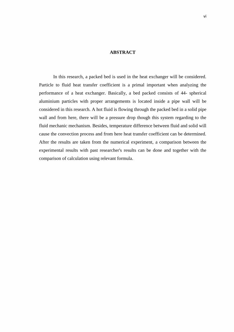
In this research, a packed bed is used in the heat exchanger will be considered.

Particle to fluid heat transfer coefficient is a primal important when analyzing the

performance of a heat exchanger. Basically, a bed packed consists of 44- spherical

aluminium particles with proper arrangements is located inside a pipe wall will be

considered in this research. A hot fluid is flowing through the packed bed in a solid pipe

wall and from here, there will be a pressure drop though this system regarding to the

fluid mechanic mechanism. Besides, temperature difference between fluid and solid will

cause the convection process and from here heat transfer coefficient can be determined.

After the results are taken from the numerical experiment, a comparison between the

experimental results with past researcher's results can be done and together with the

comparison of calculation using relevant formula.

vii

ABSTRAK

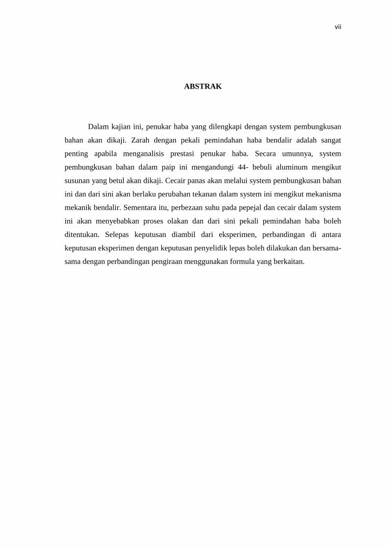
Dalam kajian ini, penukar haba yang dilengkapi dengan system pembungkusan

bahan akan dikaji. Zarah dengan pekali pemindahan haba bendalir adalah sangat

penting apabila menganalisis prestasi penukar haba. Secara umunnya, system

pembungkusan bahan dalam paip ini mengandungi 44- bebuli aluminum mengikut

susunan yang betul akan dikaji. Cecair panas akan melalui system pembungkusan bahan

ini dan dari sini akan berlaku perubahan tekanan dalam system ini mengikut mekanisma

mekanik bendalir. Sementara itu, perbezaan suhu pada pepejal dan cecair dalam system

ini akan menyebabkan proses olakan dan dari sini pekali pemindahan haba boleh

ditentukan. Selepas keputusan diambil dari eksperimen, perbandingan di antara

keputusan eksperimen dengan keputusan penyelidik lepas boleh dilakukan dan bersama-

sama dengan perbandingan pengiraan menggunakan formula yang berkaitan.

viii

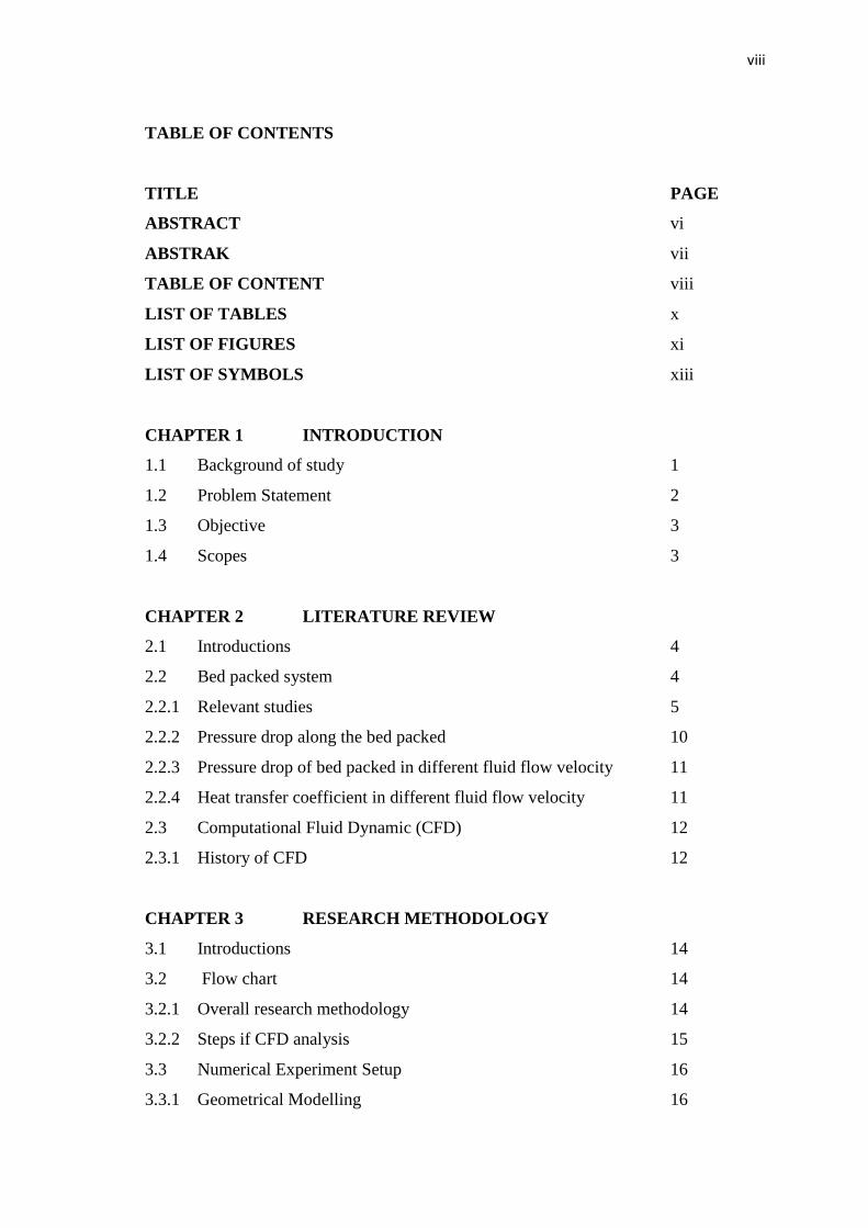
TABLE OF CONTENTS

TITLE PAGE

ABSTRACT vi

ABSTRAK vii

TABLE OF CONTENT viii

LIST OF TABLES x

LIST OF FIGURES xi

LIST OF SYMBOLS xiii

CHAPTER 1 INTRODUCTION

1.1 Background of study 1

1.2 Problem Statement 2

1.3 Objective 3

1.4 Scopes 3

CHAPTER 2 LITERATURE REVIEW

2.1 Introductions 4

2.2 Bed packed system 4

2.2.1 Relevant studies 5

2.2.2 Pressure drop along the bed packed 10

2.2.3 Pressure drop of bed packed in different fluid flow velocity 11

2.2.4 Heat transfer coefficient in different fluid flow velocity 11

2.3 Computational Fluid Dynamic (CFD) 12

2.3.1 History of CFD 12

CHAPTER 3 RESEARCH METHODOLOGY

3.1 Introductions 14

3.2 Flow chart 14

3.2.1 Overall research methodology 14

3.2.2 Steps if CFD analysis 15

3.3 Numerical Experiment Setup 16

3.3.1 Geometrical Modelling 16

ix

3.3.2 Design Modular 18

3.3.3 Mesh 18

3.3.4 Fluent 19

3.4 Apparatus 22

CHAPTER 4 RESULTS AND DISCUSSIONS

4.1 Introductions 23

4.2 Numerical experiment results 23

4.2.1 Air 23

4.2.2 Water 25

4.2.3 Nanofluid: Aluminium Oxide + Water 26

4.3 Calculation results 28

4.3.1 Calculation for air 28

4.3.2 Calculation for water 29

4.3.3 Different between calculated values and the simulation result 29

values

4.4 Comparison of numerical experiment with relevant research 30

CHAPTER 5 CONCLUSION AND RECCOMENDATIONS

5.1 Conclusions 33

5.2 Recommendation 34

REFERENCES 35

APPENDIX A: Sample of calculation 37

APPENDIX B: Simulations Results 40

x

LIST OF TABLES

TABLE NO. TITLE PAGE

1 Boundary condition for carbon dioxide 6

2 Boundary condition for air and carbon dioxide 8

3 Boundary conditions for water as fluid properties 21

4 Simulation results for air 23

5 Simulation results for water 25

6 Simulation results for different concentration of aluminium 26

oxide in water

7 Calculated Nusselt Number for air 28

8 Calculated pressure drop for water 29

9 Nanomaterial properties 30

10 Water properties 30

11 Different concentration of aluminium oxide in water properties 30

xi

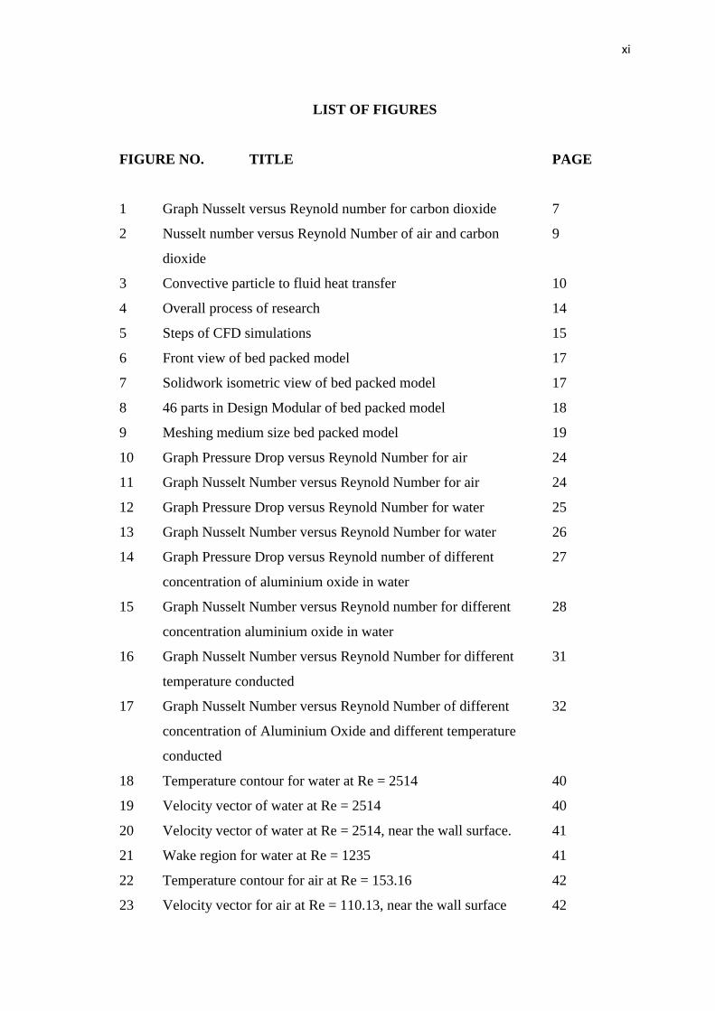
LIST OF FIGURES

FIGURE NO. TITLE PAGE

1 Graph Nusselt versus Reynold number for carbon dioxide 7

2 Nusselt number versus Reynold Number of air and carbon 9

dioxide

3 Convective particle to fluid heat transfer 10

4 Overall process of research 14

5 Steps of CFD simulations 15

6 Front view of bed packed model 17

7 Solidwork isometric view of bed packed model 17

8 46 parts in Design Modular of bed packed model 18

9 Meshing medium size bed packed model 19

10 Graph Pressure Drop versus Reynold Number for air 24

11 Graph Nusselt Number versus Reynold Number for air 24

12 Graph Pressure Drop versus Reynold Number for water 25

13 Graph Nusselt Number versus Reynold Number for water 26

14 Graph Pressure Drop versus Reynold number of different 27

concentration of aluminium oxide in water

15 Graph Nusselt Number versus Reynold number for different 28

concentration aluminium oxide in water

16 Graph Nusselt Number versus Reynold Number for different 31

temperature conducted

17 Graph Nusselt Number versus Reynold Number of different 32

concentration of Aluminium Oxide and different temperature

conducted

18 Temperature contour for water at Re = 2514 40

19 Velocity vector of water at Re = 2514 40

20 Velocity vector of water at Re = 2514, near the wall surface. 41

21 Wake region for water at Re = 1235 41

22 Temperature contour for air at Re = 153.16 42

23 Velocity vector for air at Re = 110.13, near the wall surface 42

xii

24 Temperature contour for 2% concentration of aluminium oxide 43

in water at Re = 2658

25 Temperature contour for 4% concentration of aluminium oxide 43

in water at Re = 4505

xiii

LIST OF SYMBOLS

D= effective particle diameter

= specific surface of a particle

Sp = surface area of particle

Vp = volume of particle

ρ = fluid density

ε = dimensionless void fraction

μ = fluid viscosity

fp = friction factor

Re = Reynold Number

Nu = Nusselt Number

St = Stranton number

C7H8 = toluene

= aluminium oxide

H = height of bed

ΔP = pressure drop

v = velocity of fluid

Cnf = specific heat of nanofluid

ρnf = density of nanofluid

Knf = thermal conductivity of nanofluid

μnf = viscosity of nanofluid

Φ = percentage of concentration of nanomaterial in nanofluid

φ = amount of concentration nanomaterial in nanofluid (in percentage)

1

CHAPTER 1

INTRODUCTIONS

1.1 BACKGROUND OF STUDY

The convective coefficients of a packed bed heat exchanger are important in

many process heat transfer equipment. As an example, within a heat exchanger the

evaluation of temperature profile as well as the heat transfer rates of the bed packed is

essential to control the performance of the heat exchanger. Hence, in this study is

required to develop a packed bed heat exchanger model with suitable software for the

estimation of heat transfer coefficients using water as the working fluid. Fluid may be

heated from the wall while flowing through the packed bed system.

From here, by applying the theory of heat flow or the movement of thermal

energy from place to place, heat is transferred in three methods that are conduction,

convection and radiation. Conduction is heat transfer requires the physical contact of

two objects. In the case of a wall, heat is conducted through the layers within the wall

from the warmer side to the cooler side. Meanwhile, convection is heat transfer due to

fluid or air flow. In here, heat is transferred from the wall of water is called as

convection. For radiation, heat is transferred when surfaces exchange electromagnetic

waves, such as light, infrared radiation, UV radiation or microwaves. Although

radiation does not require any fluid medium or contact, but does require an air gap or

other transparent medium between the surfaces exchanging radiation.

In such a packed bed operated under steady-state conditions, a difference in

local temperature between the fluid and the particle may exist, but the overall solid and

fluid temperature profiles are considered to be identical to each other. The temperature

profiles in the bed are then predicted in terms of effective thermal conductivities and

2

wall heat transfer coefficients. An extensive review of the aforementioned can be found

in Wakao and Kuguei, 1982.

A Computerized Fluid Dynamic (CFD) simulation is a most suitable strategy for

the estimation of effective thermal conductivities as well as wall heat transfer

coefficients. CFD is a tool uses numerical methods and algorithms to analyze systems

involving fluid flow, heat transfer and associated phenomena such as chemical reactions

by means of computer based simulation. The simulation of CFD is performed using the

FLUENT software. CFD allows us to obtain a more accurate view of the fluid flow and

heat transfer mechanisms present in packed bed heat exchanger.

Fluent is a computer program for modeling fluid flow and heat transfer in

complex geometries. Fluent provides complete mesh flexibility, including the ability to

solve your flow problems using unstructured meshes that can be generated about

complex geometries with relative ease. Fluent also allows you to refine your grid based

on the flow solution.

1.2 PROBLEM STATEMENT

The problems begin with a hot fluid is flowing through a hollow tube pipe with a

packing material inside the pipe. The packing materials are spherical solid materials.

The fluid is flowing through each spherical packing material through the column of the

packing material. The energy of the hot fluid is transferred to the solid sphere through

the convection process. The differences of temperature of the pipe wall and the fluid

also make the energy transfer of fluid to the wall. Those energy transfers are simulated

using the Fluent software in computational fluid dynamic (CFD). Although the

simulated results are not as accurate as physical experiment results but simulated results

are almost can be referred results. CFD simulations are relatively inexpensive because

the cost of the powerful computer to simulate the design can be cheaper than the

experimental solution. CFD simulations can be executed in a short period of time.

Hence, the fastest and almost an accurate way to solve that problem or through the

computer software and using CFD simulation.

3

1.3 OBJECTIVE

To determine convective heat transfer coefficient and pressure drop of a packed bed

heat exchanger using Fluent software.

1.4 SCOPES

1. Develop the model of a packed bed system in Solidwork or any other

commercial software available compatible with CFD package

2. Import the model and initialize for boundary conditions. Process/ Execute the

model using the properties of water

3. The experimental data available for the water is to be validated with

computational results for heat transfer coefficients

4. Evaluate the numerical heat transfer coefficient for nanofluid using the

properties developed in the form of equations.

4

CHAPTER 2

LITERATURE REVIEWS

2.1 INTRODUCTIONS

The aim of this chapter is to provide the past research about the bed packed

system and computational fluid dynamics (CFD) analysis in three dimension model. In

order to understand more on this research and to achieve the objective of the research,

reviewing back past research studies are needed to provide more useful information and

point.

2.2 BED PACKED SYSTEM

Bed packed system is a hallow tube filled with fixed layer of small particles or

packing material. The packing material can be any sizes and shapes but for this research,

it is spherical aluminum particles and a fluid is flowing through the bed packed particles.

The purpose of this system is to use for processes involving absorption, absorption of a

solute, distillation, filtration and separation (Geamkoplis, p.125). One of the studies in

this research is pressure drop. It is because pressure drop is important to determine the

energy requirement to pump a fluid at any bed packed system. Besides, from the

viewpoint of fluid dynamics, the most important cases are the pressure drop required for

fluid to flow through the column at a specified flow rate.

In order to calculate this amount, we are dependent on the correlation of

coefficient friction due to the Ergun. Ergun relates the flows and pressure drops to a

Reynolds number and friction factor respectively. The Reynolds number for packed

5

beds, Rep, depends upon the controlled variable and the system parameters ρ, ε, μ,

and D and is defined as (Bird et al., 1996):

=

where, D is effective particle diameter =

, is specific surface of a particle = Sp / Vp ,

Sp is surface area of particle and Vp is volume of particle. ρ is the fluid density, ε is the

dimensionless void fraction defined as the volume of void space over the total volume

of packing, and μ is the fluid viscosity.

The friction factor, fp, in the Ergun equations for Reynolds‘s number range

between 1 and 2500 are:

=

+ 1.75

2.2.1` Relevant Studies

In ―CFD studies on particle-to-fluid mass and heat transfer in packed beds: Free

convection effects in supercritical fluids‖ by Guardo. A, Coussirat. M, Recasens. F,

Larrayoz. M. A, Escaler. X have checked CFD capabilities for predicting particle-to-

fluid mass/heat transfer coefficients when a supercritical fluid was used as a solvent in a

packed bed reactor. First, numerical simulations are presented for validation model

cases (forced convection at low pressure). Numerical simulation is done to model the

mass transfer of mixed convection under high pressure, the analysis results was

obtained was compared with experimental data previously issued by (Stüber et al.,

1996), and to the heat transfer analogy proposed by (Guardo et al., 2006). Numerical

results obtained presented in this study, to validate the idea that the modified correlation

presented by (Guardo et al., 2006) can be used to describe the phenomenon of heat

transfer in packed bed under mixed convection regime at high pressures. The boundary

conditions in this study are as follow

6

Table 1: Boundary condition for carbon dioxide

Boundary condition Low pressure High

pressure

Mass transfer simulations

Circulating fluid CO2

C7H8 concentration at inlet (mol/m3) 0

C7H8 concentration at particle surface (equilibria)

(mol/m3)

5.95 120–190

Pressure (Pa) 101325 9–9.2×106

Mass flow at the inlet – 0.015–0.100

Velocity at the inlet (m/s) 7.5×10-4

–

7.5×10-1

–

Heat transfer simulations

Circulating fluid Air CO2

Temperature at the inlet (K) 298 330

Temperature at particle surface (K) 423 340

Pressure (Pa) 101325 1×107

Mass flow at the inlet – 0.013–0.132

Velocity at the inlet (m/s) 3×10-4

–7.5×10-1

–

The fluid was taken to be incompressible, Newtonian, and in a laminar or turbulent flow

regime. CO2, air and toluene at standard conditions were chosen as the simulation fluids.

Incompressible ideal gas law for density and viscosity were applied to the model for the

production of these variables depends on temperature. For the high-pressure simulations,

the fluid was taken to Newtonian, in laminar flow regime and with variable density.

CO2 and toluene, property that has been incorporated into the solver code using the

(UDE) user-defined functions and user-defined formula (UDF) was chosen as a fluid

simulation in this case, under high pressure.

7

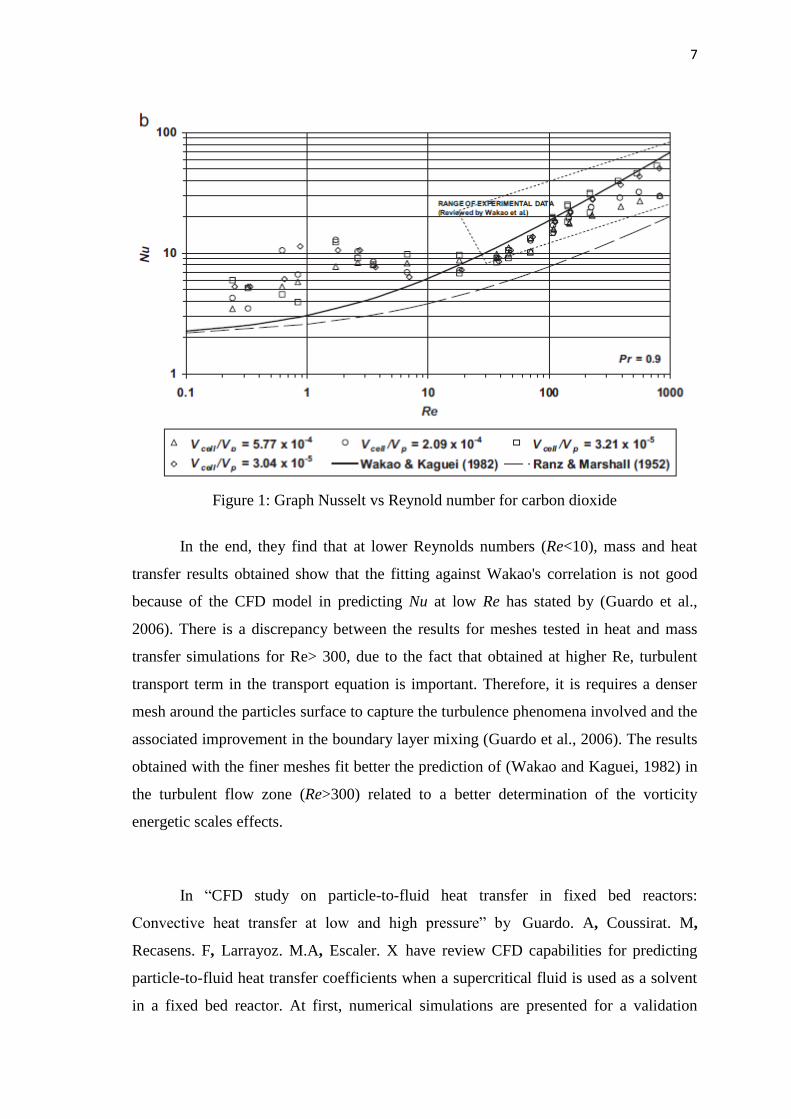
Figure 1: Graph Nusselt vs Reynold number for carbon dioxide

In the end, they find that at lower Reynolds numbers (Re<10), mass and heat

transfer results obtained show that the fitting against Wakao's correlation is not good

because of the CFD model in predicting Nu at low Re has stated by (Guardo et al.,

2006). There is a discrepancy between the results for meshes tested in heat and mass

transfer simulations for Re> 300, due to the fact that obtained at higher Re, turbulent

transport term in the transport equation is important. Therefore, it is requires a denser

mesh around the particles surface to capture the turbulence phenomena involved and the

associated improvement in the boundary layer mixing (Guardo et al., 2006). The results

obtained with the finer meshes fit better the prediction of (Wakao and Kaguei, 1982) in

the turbulent flow zone (Re>300) related to a better determination of the vorticity

energetic scales effects.

In ―CFD study on particle-to-fluid heat transfer in fixed bed reactors:

Convective heat transfer at low and high pressure‖ by Guardo. A, Coussirat. M,

Recasens. F, Larrayoz. M.A, Escaler. X have review CFD capabilities for predicting

particle-to-fluid heat transfer coefficients when a supercritical fluid is used as a solvent

in a fixed bed reactor. At first, numerical simulations are presented for a validation

8

model case (single sphere model), and next is presenting convective particle-to-fluid

heat transfer at low pressure. The results obtained are used to analyze mesh dependence

of the numerical results at low flow velocities. Finally, mixed convection at high

pressure is modeled and analyzed. Numerical results obtained are compared to accepted

correlations and a CFD-based correlation for particle-to-fluid heat transfer at high

pressure is presented. The boundary conditions are;

Table 2: Boundary condition for air and carbon dioxide

Boundary condition Low pressure High pressure

Circulating fluid Air CO2

Temperature at the inlet, K 298 330

Temperature at packing surface, K 423 340

Pressure, Pa 101 325 1×107

Mass flow at the inlet, kg/m2s — 0.013–0.132

Velocity at the inlet, m/s 3×10-4

–7.5×10-1

—

Model consists of a single sphere suspended in a box. In the CFD model the infinite

fluid was limited in a box with a square flow inlet plane of seven sphere diameters and a

length of 16 sphere diameters to keep the model reasonable in size (Nijemeisland, 2000).

To discard the presence of wall effects on temperature and velocity profiles, models

with flow inlet planes with sizes of 2, 3, 4, 6, 8 and 9 diameters were created. An

unstructured tetrahedral mesh is built in the fluid region. No mesh is built in the sphere

interior. The sphere in the box was designed with the same dimensions as the spheres

used in the fixed bed model.

9

Figure 2: Nusselt number versus Reynold Number for air and carbon dioxide

From the results, they notice that in the laminar flow and transition zone (Re

<300), the results not depending on the mesh density. At lower Reynolds numbers (Re

<10) shows the results that the fitting against (Wakao, 1976) the correlation is not good.

For a single velocity condition different meshes give results in a wide range of Nu and

no relationship with mesh density can be determined.

There is a divergence between the results obtained for tested meshes for higher values

of Re, due to the fact at higher Re, turbulent transport term in the transport equation

need to consider. An accurate turbulence modeling requires a denser mesh around the

particles surface in order to capture in a more suitable way the involved turbulence

phenomena in the boundary layer (Guardo et al., 2005). A divergence in the results

obtained with the low density meshes and the high density meshes can be seen for

Re>300.

In ―Heat and Flow Characteristics of Packed Bed by (Achenbach. E, 1995),

mass transfer experiments with single spheres are preferably conducted according to the

method of naphthalene sublimation in air. The majority of the present experiments were

conducted using a bed diameter of D = 0.983 m and a bed height of H = 0.84 m. To

eliminate wall effects, the core wall was structured such that a regular orientation of the

10

spheres adjacent to the wall was avoided. The sphere diameter was d = 0.06 m. The void

fraction was experimentally determined to be 0.387. The heat transfer experiments were

carried out by applying the method of the electrically heated single sphere in an

unheated packing. The test spheres were manufactured from copper, the surface being

highly polished and covered with a silver layer to keep the contribution of thermal

radiation low.

Figure 3: Convective particle to fluid heat transfer

2.2.2 Pressure drop along the bed packed

The increasing of pressure drop along the bed pack is due to the wake region is

created by each solid particle in the bed packed when water flow pass through it. Wake

region is a recirculating flow immediately behind a moving or stationary solid body and

it is caused by the flow of surrounding fluid around the body. The pressure is a

maximum at the stagnation point (first point contact of fluid and spherical particles) and

gradually decreases along the front half of the spherical particles of bed packed. The

pressure starts to increase in the rear half of the spherical particles of bed packed and

the particle now experiences an adverse pressure gradient. Consequently, the flow

11

separates from the surface and creating a highly turbulent region behind the spherical

particles of bed packed called the wake region. The pressure inside the wake region

remains low as the flow separates and a net pressure force (pressure drag) is produced.

2.2.3 Pressure drop of bed packed in different fluid flow velocity

The increasing pressure drop in different velocity is because of increasing of

velocity is directly proportional to increasing of pressure drop value in pressure drop

formula.

Pressure drop can be calculated using the following formula:

ΔP =

Where;

ΔP = pressure drop in Pascals (Pa)

v = velocity in metres per second (m/sec)

f = friction factor

L = length of pipe in metres (m)

ρ = density of the fluid in kilograms per cubic metre

= inside diameter of pipe in metres (m)

Hence, when the velocity of the fluid is increasing, the pressure drop values are also

increasing.

2.2.4 Heat transfer coefficient in different fluid flow velocity

All the graph of Nusselt number versus Reynold number in different fluid

properties must shows the increasing pattern. It is because due to the convection process

between fluid and the bed packed. Convection is the mode of energy transfer between

solid surface and the adjecent fluid in motion and it involves combined effect of

conduction and fluid motion. Hence, the faster the fluid motion, the greater the

convection heat transfer and the higher the Nusselt number will be.

12

2.3 COMPUTATIONAL FLUID DYNAMICS (CFD)

Computational fluid dynamics (CFD) is the science of predicting fluid flow, heat

and mass transfer, chemical reactions, and related phenomena by solving numerically

the set of governing mathematical equations. CFD provides numerical approximation to

the equations that govern fluid motion. These equations are then discretized to produce

a numerical analogue of the equations.

All CFD codes contain three main elements:

1. A pre-processor, which is used to input the problem geometry, generate the grid,

define the flow parameter and the boundary conditions to the code.

2. A flow solver, which is used to solve the governing equations

of the flow subject to the conditions provided. There are four different methods

used as a flow solver: (i) finite difference method; (ii) finite element method, (iii)

finite volume method, and (iv) spectral method.

3. A post-processor, which is used to massage the data and show the results in

graphical and easy to read format.

2.3.1 History of CFD

In England, Lewis Fry Richardson (1881-1953) developed the first numerical

weather prediction system CFD approximation in 1922 when he divided physical space

into grid cells and used the finite difference approximations of Bjerknes's "primitive

differential equations". His own attempt to calculate weather for a single eight-hour

period took six weeks and ended in failure. His model's enormous calculation

requirements led Richardson to propose a solution he called the "forecast-factory". The

"factory" would have involved filling a vast stadium with 64,000 people. Each one,

armed with a mechanical calculator, would perform part of the flow calculation. A

leader in the centre, using coloured signal lights and telegraph communication, would

coordinate the forecast. What he was proposing would have been a very rudimentary

CFD calculation. The earliest numerical solution for flow pass a cylinder is in 1933 that

is by Thom. A, publishing ‗The Flow Past Circular Cylinders at Low Speeds‘, Proc.

Royal Society, A141, pp. 651-666, London, 1933.

13

During the 1960s, the theoretical division of NASA at Los Alamos in the U.S.

contributed many numerical methods that are still in use in CFD today, such as the

following methods: Particle-In-Cell (PIC), Marker-and-Cell (MAC), Vorticity- Stream

function methods, Arbitrary Lagrangian-Eulerian (ALE) methods, and the ubiquitous k

- e turbulence model. In the 1970s, a group working under D. Brian Spalding, at

Imperial College, London, developed Parabolic flow codes (GENMIX), Vorticity-

Stream function based codes, the SIMPLE algorithm and the TEACH code, as well as

the form of the k - e equations that are used today (Spalding & Launder, 1972). They

went on to develop Upwind differencing, 'Eddy break-up' and 'presumed PDF'

combustion models. Another event of CFD industry was in 1980 when Suhas V.

Patankar published ―Numerical Heat Transfer and Fluid Flow", probably the most

influential book on CFD to date, and the one that spawned a thousand CFD codes.

It was in the early 1980s that commercial CFD codes came into the open market

place in a big way. The use of commercial CFD software started to become accepted by

major companies around the world rather than their continuing to develop in-house

CFD codes. Commercial CFD software is therefore based on sets of very complex non-

linear mathematical expressions that define the fundamental equations of fluid flow,

heat and materials transport. These equations are solved iteratively using complex

computer algorithms embedded within CFD software. The net effect of such software is

to allow the user to computationally model any flow field provided the geometry of the

object being modelled is known, the physics and chemistry are identified, and some

initial flow conditions are prescribed.

CFD is now recognized to be a part of the computer-aided engineering

(CAE) spectrum of tools used extensively today in all industries, and its approach to

modeling fluid flow phenomena allows equipment designers and technical analysts to

have the power of a virtual wind tunnel on their desktop computer.

14

CHAPTER 3

METHODOLOGY

3.1 INTRODUCTIONS

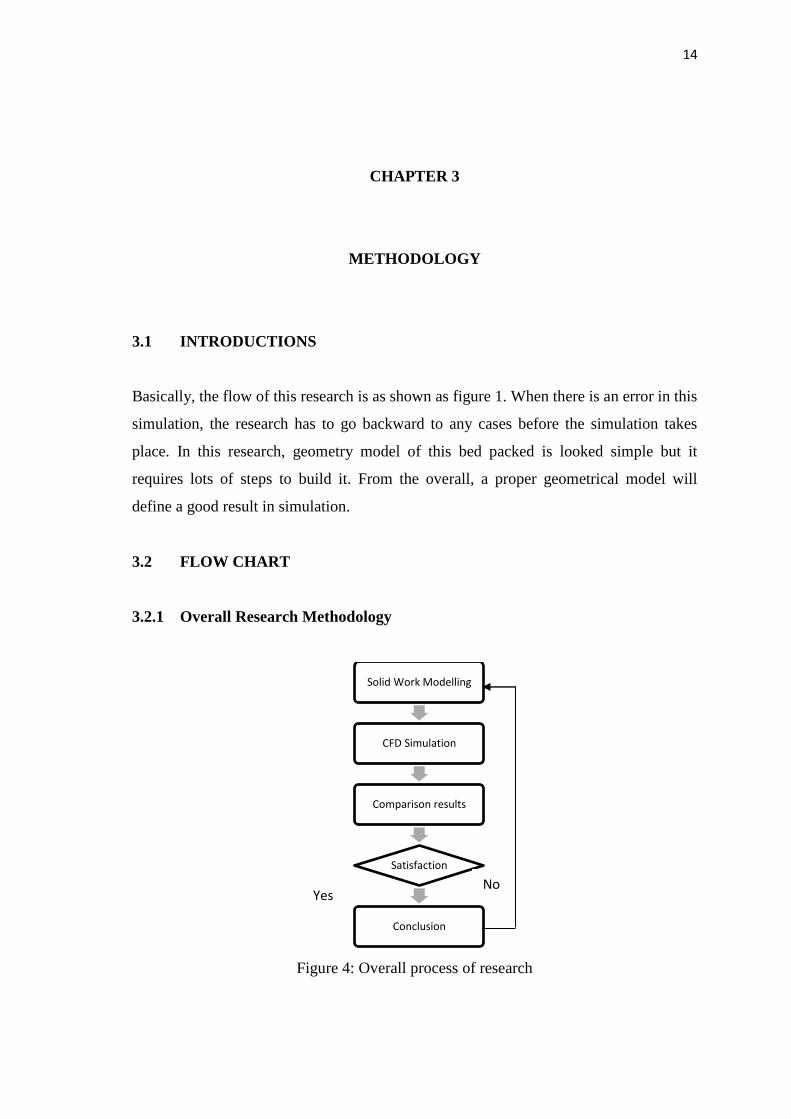
Basically, the flow of this research is as shown as figure 1. When there is an error in this

simulation, the research has to go backward to any cases before the simulation takes

place. In this research, geometry model of this bed packed is looked simple but it

requires lots of steps to build it. From the overall, a proper geometrical model will

define a good result in simulation.

3.2 FLOW CHART

3.2.1 Overall Research Methodology

Figure 4: Overall process of research

Solid Work Modelling

CFD Simulation

Comparison results

Satisfaction

Conclusion

Yes No

15

3.2.2 Steps of CFD analysis

Figure 5: Steps of CFD simulations

Transfered model from Solid Work to Design Modular

Transfer data from Design Modular to Mesh

Apply the mesh and grid to the model

Transfer mesh model to FLUENT

Set up the properties and boundary conditions of the model

Validate the results and discuss the result

Satisfaction

Conclude the simulation results

No

Yes