Embed Size (px)
Citation preview

Cesar Morais Palomo
Interactive image-based rendering for virtualview synthesis from depth images
MSc Thesis
Thesis presented to the Post–graduate Program in ComputerScience of the Computer Science Department, PUC–Rio as par-tial fulfillment of the requirements for the degree of Master inComputer Science
Adviser: Prof. Marcelo Gattass
Rio de JaneiroJuly 2009


Cesar Morais Palomo
Interactive image-based rendering for virtualview synthesis from depth images
Thesis presented to the Post–graduate Program in ComputerScience of the Computer Science Department, PUC–Rio as par-tial fulfillment of the requirements for the degree of Master inComputer Science. Approved by the following commission:
Prof. Marcelo Gattass
AdviserDepartment of Computer Science — PUC–Rio
Prof. Alberto Barbosa Raposo
Computer Science Department — PUC-Rio
Prof. Waldemar Celes Filho
Computer Science Department — PUC-Rio
Prof. Paulo Cezar Pinto Carvalho
Visgraf Laboratory — IMPA
Rio de Janeiro — July 06, 2009


All rights reserved.
Cesar Morais Palomo
Cesar Morais Palomo graduated from the State University ofCampinas with a BSc. in Computer Science in 2005. From2002 to 2007 he worked as a contractor for several companiesas a software engineer, designing and developing enterpriseand critical systems for the industry and the Brazilian govern-ment. In 2007 he started the graduate program in ComputerScience at PUC-Rio as a master candidate. In the same year,he joined the Computer Graphics Technology Group (Tec-graf), where he has been developing computer systems in thefields of computer graphics visualization, computer vision, vir-tual and augmented reality.
Bibliographic data
Palomo, Cesar M.
Interactive image-based rendering for virtual view synthe-sis from depth images / Cesar Morais Palomo; adviser: Mar-celo Gattass. — Rio de Janeiro : PUC–Rio, Department ofComputer Science, 2009.
v., 60 f: il. ; 29,7 cm
1. MsC Thesis - Pontifıcia Universidade Catolica do Riode Janeiro, Department of Computer Science.
Bibliography included.
1. Computer Science – Dissertation. 2. Image-based ren-dering. 3. Blending. 4. GPU programming. 5. Depth images.I. Gattass, M.. II. Pontifıcia Universidade Catolica do Rio deJaneiro. Department of Computer Science. III. Title.
CDD: 004


Acknowledgments
Abstract
Palomo, Cesar M.; Gattass, M.. Interactive image-based ren-dering for virtual view synthesis from depth images. Rio deJaneiro, 2009. 60p. MScThesis — Department of Computer Science,Pontifıcia Universidade Catolica do Rio de Janeiro.
Image-based modeling and rendering has been a very active research topic
as a powerful alternative to traditional geometry-based techniques for image
synthesis. In this area, computer vision algorithms are used to process and
interpret real-world photos or videos in order to build a model of a scene,
while computer graphics techniques use this model to create photorealistic
images based on the captured photographs or videos.
The purpose of this work is to investigate rendering techniques capable of
delivering visually accurate virtual views of a scene in real-time.
Even though this work is mainly focused on the rendering task, without the
reconstruction of the depth map, it implicitly overcomes common errors in
depth estimation, yielding virtual views with an acceptable level of realism.
Tests with publicly available datasets are also presented to validate our
framework and to illustrate some limitations in the IBR general approach.
Keywords
Image-based rendering. Blending. GPU programming. Depth ima-
ges.

Resumo
Palomo, Cesar M.; Gattass, M.. Renderizacao interativa base-ada em imagens para sıntese de vistas virtuais a partir deimagens com profundidade. Rio de Janeiro, 2009. 60p. Dissertaode Mestrado — Departamento de Informatica, Pontifıcia Universi-dade Catolica do Rio de Janeiro.
Modelagem e renderizacao baseadas em imagem tem sido uma area de pes-
quisa muito ativa nas ultimas decadas, tendo recebido grande atencao como
uma alternativa as tecnicas tradicionais de sıntese de imagens baseadas pri-
mariamente em geometria. Nesta area, algoritmos de visao computacional
sao usados para processar e interpretar fotos ou vıdeos do mundo real a fim
de construir um modelo representativo de uma cena, ao passo que tecnicas
de computacao grafica sao usadas para tomar proveito desta representacao
e criar cenas foto-realistas.
O proposito deste trabalho e investigar tecnicas de renderizacao capazes de
gerar vistas virtuais de alta qualidade de uma cena, em tempo real. Para
garantir a performance interativa do algoritmo, alem de aplicar otimizacoes
a metodos de renderizacao existentes, fazemos uso intenso da GPU para o
processamento de geometria e das imagens para gerar as imagens finais.
Apesar do foco deste trabalho ser a renderizacao, sem reconstruir o mapa
de profundidade a partir das fotos, ele implicitamente contorna possıveis
problemas na estimativa da profundidade para que as cenas virtuais geradas
apresentem um nıvel aceitavel de realismo.
Testes com dados publicos sao apresentados para validar o metodo pro-
posto e para ilustrar deficiencias dos metodos de renderizacao baseados em
imagem em geral.
Palavras–chave
Renderizacao Baseada em Imagens. Composicao. Programacao em
placas graficas. Mapa de profundidade.


Contents
1 Introduction 15
2 Related Work 192.1 IBR real applications 192.2 Static scenes 212.3 Dynamic scenes 23
3 Rendering depth images 273.1 Image acquisition process 273.2 Depth image representation 293.3 3D warping 303.4 Artifacts inherent to 3D warping 31
4 Compositing 354.1 Virtual camera navigation 354.2 Blending algorithm 374.3 Limitations 38
5 IBR on the GPU 415.1 Conceptual algorithm 415.2 Creation of view-dependent geometry 425.3 Warping to novel viewpoint and occlusions identification 435.4 Compositing on the GPU 44
6 Results 496.1 Rendering quality 496.2 Limitations 526.3 Time-performance analysis 536.4 Summary 54
7 Conclusion and Future works 55
Bibliography 57

List of Figures
1.1 Skin and hair rendering are examples of challenges to purelygeometry-based approaches. 15
1.2 Plenoptic function. 16
2.1 Bullet-time effect shows the necessity of counterbalancing thenumber of input cameras and quality of rendered images. 20
2.2 IBR goals: establish mapping between representation and imagescreen, and blend. 21
2.3 Layered Depth Images [30]. Input images (left) used to generatethe layered representation of a scene (top right). It allows forreconstruction of views free from disocclusion problems (bottom). 22
2.4 View-dependent texture mapping [11]. Input images are projectedonto reconstructed architectural model, and assembled to form acomposite rendering. Top two pictures show images projected ontomodel, lower left shows results of blending those two renderings,and lower right shows final result of blending a total of 12 originalimages. 23
2.5 Kanade et al’s Virtualized Reality geodesic dome [17]. 242.6 Goldlucke results [13]. The regular triangular mesh causes inaccu-
rate appearance at the vicinity of depth discontinuities. 252.7 Camera setup in Zitnick et al [38]. Eight cameras are used to
capture 1024x768 images, synchronized with commissioned PtGreyconcentrator units. 26
2.8 Rendering results for Zitnick et al [38]: (a) main layer M fromone view rendered, with depth discontinuities erased; (b) boundarylayer B rendered; (c) main layer M for other view rendered; (d) finalblended result. 26
3.1 Imaging process in the pinhole camera model: image formationis a sequence of transformations between coordinate systems. Weignore here radial distortion. 27
3.2 Example of a depth image: color image + dense depth map. Darkerpixels in depth map mean greater depth. Courtesy of Zitnick et al[38]. 29
3.3 3D warping process. First, 3D mesh generated using depth mapfrom reference camera Ci is unprojected to global coordinatesystem. Then, mesh is projected into a virtual view using cameraCvirtual projection matrix. 30
3.4 3D warping result. Depth image (pair of images to the left) froma reference camera is projected into a virtual view (right image)using the described 3D warping process. In this case, virtual cameraCvirtual was placed slightly to the right of reference camera Ci. 32

3.5 3D warping artifacts due to discontinuity in depth. The continuityassumption in depth map does not hold at objects’ boundaries,which causes undesirable artifacts in the form of stretched trianglesin warped view. When depth map (left) is warped to new viewpoint,the region to the right of the ballet dancer reveals occluded areas. 32
3.6 3D warping to a new viewpoint, with occluded regions drawn inblack thank to our labeling schema. 33
4.1 Example of cameras setup: input cameras arranged along a 1D arc. 364.2 Navigation of virtual camera Cvirtual restricted to the lines linking
center of adjacent pair of input cameras. 364.3 Virtual camera’s parameters can be determined as a linear interpo-
lation of adjacent pair of cameras. 364.4 Blending algorithm. Two reference views Ci and Ci+1, adjacent to
virtual viewpoint Cvirtual, are used in composition stage. 374.5 Cases considered in the compositing process. 394.6 Frontier r between regions A and B may become undesirably visible
due to the stepped behavior of our compositing algorithm and thereexist photometric (e.g. gain) differences in cameras used for capture. 39
4.7 Visible seams between occlusion and blended areas, to the rightand to the left of woman’s head. 40
5.1 Conceptual algorithm for novel view synthesis. 415.2 Vertex-buffer object used for improving performance during mesh
generation. 435.3 Reference view rendering into a FBO, using vertex and fragment
shaders. 445.4 Influence of angular distance in reference camera’s contribution
during compositing. 455.5 Penalty for pixels marked occluded based on angular distance. 46
6.1 Sample data from Ballet (left) and Breakdancers(right) sequences:color images on top, and corresponding depth images below [38]. 50
6.2 Synthesized images for one frame of ballet sequence. Left and mid-dle columns respectively correspond to cameras’ 5 and 4 warpingresults, and right column is the final result. First row: occlusion ar-eas not identified and rubber sheets appear. Second row: we applythe proposed labeling approach. 50
6.3 Synthesized images for one frame of breakdancers sequence. Leftand middle columns respectively correspond to cameras’ 3 and 2warping results, and right column is the final result. First row:occlusion areas not identified and rubber sheets appear. Secondrow: we apply the proposed labeling approach. 50
6.4 Virtual camera positioned coincidently with camera’s 5 position inballet sequence, and cameras 5 and 6 used as reference cameras.Left column: original image. Middle column: synthetic image. Rightcolumn: differences between real and synthetic images. Negated forease of printing: equal pixels in white. 51

Interactive image-based rendering for virtual view synthesis from depth images 14
6.5 Virtual camera positioned coincidently with camera’s 5 position inballet sequence, and cameras 5 and 6 used as reference cameras.Left column: original image. Middle column: synthetic image. Rightcolumn: differences between real and synthetic images. Negated forease of printing: equal pixels in white. 51
6.6 Close-up of rendering result for frame 48 in ballet sequence. Leftcolumn: original photo from camera 7. Middle column: estimateddepth map. Right column: visible seams below dancer caused bywrong depth estimates. 52
6.7 Close-up of rendering result for frame 88 in breakdancers sequence.Left column: original photo from camera 7. Middle column: esti-mated depth map. Right column: visible seams close to dancer’sfoot caused by wrong depth estimates. 52
6.8 Close-ups of rendering artifacts (shadowing) for frame 48 in balletsequence and frame 88 in breakdancers sequence. 53
6.9 Close-ups of rendering artifacts (due to matting absence) for frame48 in ballet sequence and frame 88 in breakdancers sequence. 53
6.10 Render time X input images’ number of pixels. 54
1
Introduction
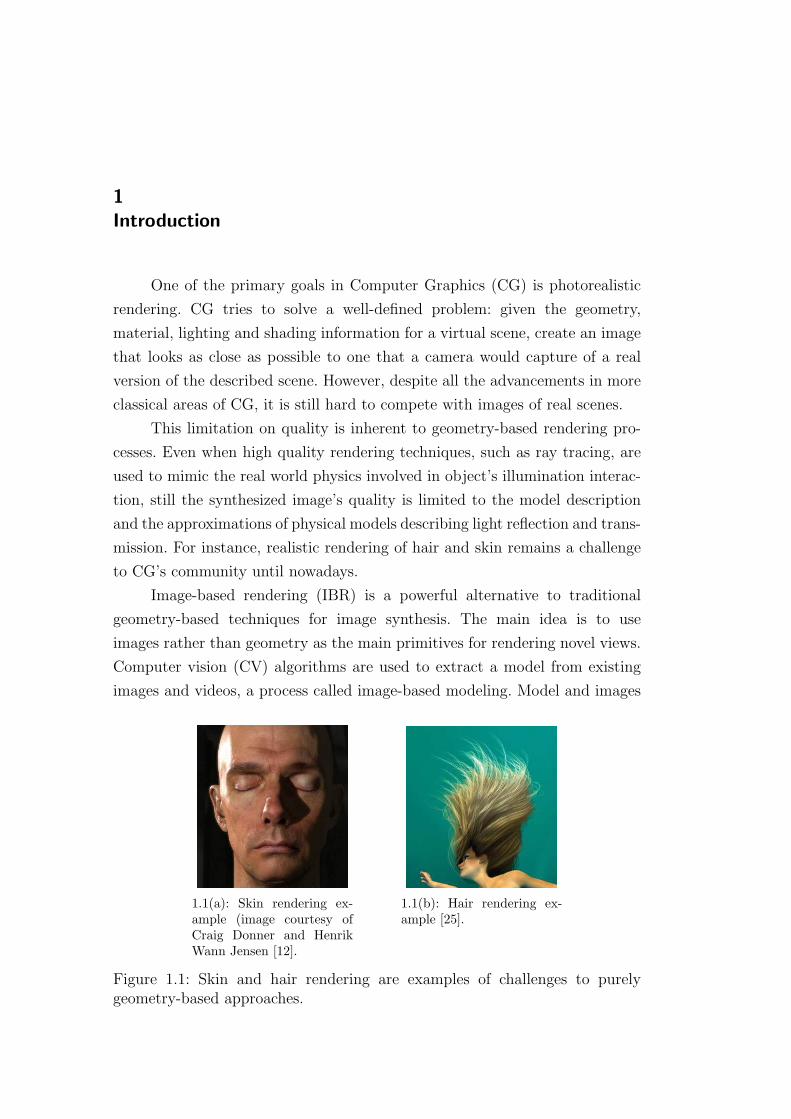
One of the primary goals in Computer Graphics (CG) is photorealistic
rendering. CG tries to solve a well-defined problem: given the geometry,
material, lighting and shading information for a virtual scene, create an image
that looks as close as possible to one that a camera would capture of a real
version of the described scene. However, despite all the advancements in more
classical areas of CG, it is still hard to compete with images of real scenes.
This limitation on quality is inherent to geometry-based rendering pro-
cesses. Even when high quality rendering techniques, such as ray tracing, are
used to mimic the real world physics involved in object’s illumination interac-
tion, still the synthesized image’s quality is limited to the model description
and the approximations of physical models describing light reflection and trans-
mission. For instance, realistic rendering of hair and skin remains a challenge
to CG’s community until nowadays.
Image-based rendering (IBR) is a powerful alternative to traditional
geometry-based techniques for image synthesis. The main idea is to use
images rather than geometry as the main primitives for rendering novel views.
Computer vision (CV) algorithms are used to extract a model from existing
images and videos, a process called image-based modeling. Model and images
1.1(a): Skin rendering ex-ample (image courtesy ofCraig Donner and HenrikWann Jensen [12].
1.1(b): Hair rendering ex-ample [25].
Figure 1.1: Skin and hair rendering are examples of challenges to purelygeometry-based approaches.

Interactive image-based rendering for virtual view synthesis from depth images 16
Figure 1.2: Plenoptic function.
then work as input for rendering methods that can take advantage of real-world
samples of the scene’s radiance and lighting properties, potentially leveraging
synthesized images higher visual accuracy.
Ideally, the obtained model describing a scene would be equivalent to the
plenopticfunction [3]:P7(θ, φ, λ, t, Vx, Vy, Vz) (1-1)
To measure this 7D function, one can imagine placing a pinhole camera’s
center at every 3D location (Vx, Vy, Vz) at every possible angle (θ, φ), for
every wavelength λ, at every time instant t. Indeed, image-based modeling
and rendering can be defined as a means of sampling the plenoptic function,
representing it in a compact and useful manner, compressing all this data and
rendering novel views from it. In other words, IBR can be viewed as a set of
techniques to reconstruct a continuous representation of the plenoptic function
using observed samples as input.
The generation of novel views from acquired images is motivated by
several applications in computer games, sports broadcast, TV advertising,
cinema and entertainment industry. In case of ambiguity in a soccer game,
for instance, many input views may be used to synthesize a new view at a
different angle to help referees inspect for events such as fouls or offsides.
The goal of this work is to develop a method of rendering synthetic
novel views of a scene captured by real cameras, capable of generating visually
accurate images at interactive rendering rates. Depth images, i.e. color images
along with their dense depth maps, are used as the sole input of our algorithm.
Results demonstrate the efficiency and quality of the proposed system.
In short, our method has the following characteristics:
– Real-time performance for virtual view synthesis.
– Visually-accurate synthesized views: rendered images have quality com-
parable to the input photos, with few visible artifacts.

Interactive image-based rendering for virtual view synthesis from depth images 17
– Transitions between views are smooth: visible changes when changing
from one viewpoint to another are not easily noticeable.
The main contribution of this work is an IBR method running entirely
on the GPU. That not only guarantees good performance, but also leaves the
CPU free to perform other tasks like input video decoding, for instance. An
additional contribution is that our method depends solely on depth images as
input, without any pre-processing stage of the input.
This document is organized as follows. Chapter 2 presents a review of
related research in IBR, delineating reasons for our design choices. Chapters 3
and 4 present the basics on depth image representation and how images can
be composited for virtual synthesis. Chapter 5 describes how the proposed
method modifies existing techniques to better suit rendering at the GPU.
Results and performance numbers are depicted in Chapter 6, where publicly
available datasets are used to test our algorithm. Finally, in Chapter 7 we
conclude and present future work directions to further improve and extend
our architecture.


2
Related Work
In this chapter we present a brief history of IBR and review relevant
research results for free viewpoint both in static and dynamic scenes. These
works present different strategies for model acquisition, representation and
rendering. However, the review is focused especially in model representations
and corresponding rendering techniques, since our main goal is visually-
accurate rendering at interactive frame rates. We start with real applications
that greatly helped spur IBR research.
2.1
IBR real applications
Maybe one of the most popular uses of IBR was the Bullet Time Effect in
1999 movie The Matrix by Warner Bros [1]. The technique used still cameras
surrounding an object in a predefined array, forming a complex curve in space,
triggered sequentially or simultaneously. Then, singular frames taken from each
of the still cameras were arranged and displayed consecutively to produce an
orbiting viewpoint of an action frozen in time or in hyper-slow-motion.
Although the technique used in The Matrix, in theory, allowed for
limitless perspectives and variable display frame rates with a virtual camera,
those perspectives were limited to the predefined camera paths. Besides, many
input cameras and man-hours were necessary to make the virtual camera fly-
through smooth and realistic.
But it was more than one decade before The Matrix, in the early 1980’s,
that the freeze frame effect was first demonstrated by Tim Macmillan’s Time-
slice [20]. An earlier version consisted of 360 pinhole film cameras arranged in a
circle looking towards the center of a circle, where the subject was positioned.
Filming was done in the dark, using a flash. A later version reduced the number
of cameras to 120, covering 90◦.
Another similar approach was used by Dayton Taylor’s Timetrack system
to produce commercials in 1995 [34]: the illusion of moving through a frozen
slice of time was produced by rapidly jumping between different still cameras
arranged along a path, just like it would be done some years later in The

Interactive image-based rendering for virtual view synthesis from depth images 20
2.1(a): Input cameras arranged in a predefinedarray.
2.1(b): Frozen-time frame ina fly-through around thecharacter.
Figure 2.1: Bullet-time effect shows the necessity of counterbalancing thenumber of input cameras and quality of rendered images.
Matrix. Also in 1995, Michel Gondry’s ”Like a rolling Stone” music video
clip innovated by using morphing between adjacent cameras rather than just
jumping from one to another.
The freeze frame/bullet time effect attracted the interest from the re-
search community. But earliest works in IBR focused unsurprisingly on deal-
ing with static scenes. Pioneering works include Chen and Williams’ View
Interpolation [8], Chen’s QuickTime VR [7], McMillan and Bishop’s Plenoptic
Modeling [23], Levoy and Hanrahan’s Light Field Rendering [19], Gortler et
al’s Lumigraph [14].
An even more promising application of the method is Free viewpoint
TV (FTV) [33]: multi-view video and multi-view depth would be broadcasted,
allowing for a free viewpoint experience to the final spectator. Since December
2001 MPEG has been working on the exploration of 3D Audio-Visual (3DAV)
technology, and since then has received strong support from TV industry
organizations for FTV standardization.
Those works may differ in the number of image samples necessary for
obtaining good rendering results, in their representation of the scene, and in
the rendering algorithm itself. However, all of them share the general goals
of IBR depicted in Figure 2.2: create a representation linked to images of the
acquired scene, and composite views to create a new one.
Although early image-based representations that are based solely on
image samples, like Light Field Rendering and Panoramas, require very simple
rendering techniques, a great number of input samples are necessary. Later on,
more sophisticated representations were proposed to deal with the trade-off
between images and geometry, and rendering techniques changed accordingly.

Interactive image-based rendering for virtual view synthesis from depth images 21
Figure 2.2: IBR goals: establish mapping between representation and imagescreen, and blend.
2.2
Static scenes
By removing time t and light wavelength λ, in 1995 McMillan and Bishop
[23] introduced the concept of Plenoptic Modeling, with the 5D version of the
plenoptic function P5(Vx, Vy, Vz, θ, φ). An even simpler representation is the
2D panorama, where the viewpoint is fixed (P2(θ, φ)). It can be cylindrical, as
in 1995 Chen’s Quicktime VR [7], or spherical, as in 1997 Szeliski and Shum’s
work [32].
Levoy and Hanrahan’s 1996 Light field rendering system [19] constrains
the plenoptic function to a bounding box, thus representing it as a 4-dimension
function. Rays are interpolated assuming that the scene surface is close to a
focal plane. Objects surfaces located far away from the focal plane appear
blurred at interpolated views.
Lumigraph system [14], proposed in 1996, uses a similar rendering
method, also restricted to a bounding box. However, rather than Light Field’s
unique focal plane, it uses an approximation of 3D object surface to reduce
the blur problem. Still, a huge number of input images are necessary for high-
quality rendering.
Chen and Williams’ 1993 View Interpolation method [8] makes use of
implicit geometry to reconstruct arbitrary viewpoints given two input images
and dense optical flow between them. The method works well when input views
are close by. Otherwise, the overlapping parts may become too small, impairing
the dense optical flow computation.
Also using implicit geometry, Seitz and Dyers’s 1996 View Morphing
technique [29] reconstructs any viewpoint on the line that links two optical
centers of the original cameras. Intermediate views are exactly linear combi-
nations of two views given that the camera motion is perpendicular to the
camera viewing direction.
The aforementioned works either require a large number of images for
rendering (methods that do not rely on geometry) or require very accurate
image registration (methods that use implicit geometry) for high-quality

Interactive image-based rendering for virtual view synthesis from depth images 22
Figure 2.3: Layered Depth Images [30]. Input images (left) used to generatethe layered representation of a scene (top right). It allows for reconstructionof views free from disocclusion problems (bottom).
virtual synthesis. Those limitations can be overcome through the usage of
explicit 3D information, encoded either in the form of 3D coordinates or depth
along lines-of-sight.
In 1999 McMillan [22] argue that 3D warping techniques can be used to
render new viewpoints when depth information is available for every point in
images. This is accomplished by unprojecting pixels of the original images to
their proper 3D locations, and subsequently reprojecting them onto the new
viewpoint. The side-effect of that method is the appearance of holes in the
warped image.
Difference of sampling resolution (as in the case of zooming-in) or
disocclusions, i.e. depth discontinuities, are the causes of holes generation.
Splatting [15] has proved to be enough to fill holes introduced by sampling
differences, but it cannot deal with disocclusions.
Shade et al’s 1998 Layered Depth Images (LDIs) [30], proposed the
storage of depth information not only for what is visible in the input image,
but also for everything behind the visible surface. In other words, each pixel in
the input image contains a list of depth and color values. The correct position
in that list could be retrieved and used accordingly depending on the new
viewpoint’s position. This layered representation can be seen in Figure 2.3.
Another use of explicit geometry in IBR is View-dependent texture-
mapping (VDTM), proposed in 1996 by Debevec et al [11], depicted in Figure
2.4. It consists in texture-mapping 3D models of a reconstructed architecture
environment, through warping and blending of several input images of that
environment. The technique was later improved by Debevec et al [10], in 1998,
to reduce computational cost and to allow for smooth blending. The main
advantage of that approach is the usage of projective texture mapping, which
boosts performance through the usage of graphics hardware.
Regarding the composition process, the Unstructured Lumigraph [5],

Interactive image-based rendering for virtual view synthesis from depth images 23
Figure 2.4: View-dependent texture mapping [11]. Input images are projectedonto reconstructed architectural model, and assembled to form a compositerendering. Top two pictures show images projected onto model, lower left showsresults of blending those two renderings, and lower right shows final result ofblending a total of 12 original images.
proposed in 2001 by Buehler et al, presents a very detailed analysis of how
textures can be blended based on relative angular position, resolution, and
field-of-view. It is a valuable reference for more principled and visually-accurate
composition.
Finally, Kang and Szeliski [18] introduced in 2004 the idea of not only
using view-dependent textures, but also view-dependent geometries for dealing
with non-Lambertian surfaces properties. Warped depth images are blended
to produce new views that resemble original non-rigid effects very effectively.
Further research works have focused on how to handle non-rigid effects,
but works presented in this section have been successfully adapted to deal with
the more intriguing task of rendering dynamic scenes with IBR.
2.3
Dynamic scenes
As mentioned in the previous section, the bullet-time/freeze-frame effect
is a very popular application of IBR for dynamic scenes, and its popularity
helped spur IBR research on the pursuit of free viewpoint in what is called
video-based rendering (VBR) [21].
Extending IBR techniques to dynamic scenes with arbitrary viewpoint
selection while the scene is changing is not trivial, although its application is ex-
tremely attractive. Associated problems are twofold. First, there are hardware-
related issues such as camera synchronization, calibration and images acquisi-
tion and storage. Decreasing costs of hardware and technology improvements
helped make the capture and subsequent processing of dynamic scenes more
practical. Second, it is difficult to achieve automatic generation of seamless in-
terpolation between views for arbitrary scenes. Proposed techniques must deal

Interactive image-based rendering for virtual view synthesis from depth images 24
Figure 2.5: Kanade et al’s Virtualized Reality geodesic dome [17].
with those difficulties to achieve high-quality rendering at reasonable time.
One of the earliest VBR systems is Kanade et al’s 1997 Virtualized
Reality [17]. Their architecture involved 51 cameras arranged around a 5-meter
geodesic dome, as shown in Figure 2.5. Cameras captured 640x480 video at
30 fps. An important aspect to notice about their work is the two-step video
acquisition: real-time recording and an offline digitization step. Virtualized
Reality computed a dense stereo depth map for each camera, used as view-
dependent geometry for view synthesis. A first version of the system used the
closest reference view as a basis, and other two neighbor cameras for hole
filling, while a second version involved the merging of depth maps into a single
model to be textured with multiple reference views. A version named Eyevision
was successfully used commercially by CBS Television at Super Bowl XXXV
in 2001, with more than 30 cameras involved.
Vedula et al [36] extended Virtualized Reality in 2005 by employing
spatio-temporal view interpolation. It explicitly recovered 3D scene shape at
every time frame and also 3D scene flow (local instantaneous 3D non-rigid
temporal deformation). A voxelization algorithm was used for both 3D shape
extraction and rendering. For novel view generation, ray-casting along with
blending weights were used. Weights were a combination of temporal and
spatial proximity to the novel viewpoint.
Stanford Light Field Camera was proposed initially in 2002 with 6 input
cameras [37]. It was later extended in 2004 to a system with 128 CMOS
cameras [35], designed based on the IEEE 1394 high speed serial bus (Firewire).
Cameras are capable of acquiring 640x480 videos at 30 fps, with 8:1 MPEG
compression.
Goldlucke et al [13] in 2002 used a subset of Stanford Light Field Camera
for acquiring and displaying dynamic scenes. In their work, cameras calibration
is done for extrinsic and intrinsic parameters estimation, to reduce radial
distortion and also to reduce color and brightness variation across cameras.
Depth maps are obtained through depth from stereo. After depth es-

Interactive image-based rendering for virtual view synthesis from depth images 25
Figure 2.6: Goldlucke results [13]. The regular triangular mesh causes inaccu-rate appearance at the vicinity of depth discontinuities.
timation for all images and timeframes, interactive rendering is achieved by
employing 3D warping. A regular, downsampled triangle mesh is created cov-
ering each of the input depth images. A vertex program is used for warping to
the novel view, and composition of 4 different reference views is done through
weights based on proximity to the novel view: the closer the input image, the
higher its weight.
They report a frame rate of 11 fps with a mesh resolution of 160x120.
Figure 2.6 shows how the triangular mesh superimposed on a reference view’s
depth map. Since the triangular mesh is continuous and regular, at the
vicinity of big depth discontinuities the appearance is usually incorrect. In
fact, the mesh downsampling generates an unpleasant blurring effect at objects
boundaries. A great improvement regarding rendering quality is presented
by Zitnick et al [38]. Although their system is quite modest in size, with
only 8 cameras, higher resolution images (1024x768) are captured at 15 fps.
Photorealism is achieved using a two-layer representation inspired by Layered-
depth images [30], mentioned in the previous section.
Their system calculates a dense depth map for each input color image
with their proposed algorithm. After that, they divide the scene representation
in two layers: boundary layer B, around depth discontinuities, and main layer
M . To generate this representation, a variant of Bayesian matting [9] is used to
automatically estimate foreground and background colors, depths and opacities
around depth discontinuities.
System configuration is shown in Figure 2.7. At rendering time, the two
reference views nearest to the novel view are chosen, warped through usage
of a custom vertex shader into separate buffers, and finally blended through
a custom fragment shader that calculates contribution weights based on an-
gular proximity of the reference view to the novel view. Their system involves
both offline and real-time phases. Computation of depth maps, boundaries
identification and matting in those areas, compression and storage are offline
processes. Decoding and rendering are done in real-time, with reported per-
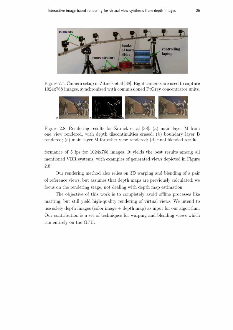
Interactive image-based rendering for virtual view synthesis from depth images 26
Figure 2.7: Camera setup in Zitnick et al [38]. Eight cameras are used to capture1024x768 images, synchronized with commissioned PtGrey concentrator units.
Figure 2.8: Rendering results for Zitnick et al [38]: (a) main layer M fromone view rendered, with depth discontinuities erased; (b) boundary layer Brendered; (c) main layer M for other view rendered; (d) final blended result.
formance of 5 fps for 1024x768 images. It yields the best results among all
mentioned VBR systems, with examples of generated views depicted in Figure
2.8.
Our rendering method also relies on 3D warping and blending of a pair
of reference views, but assumes that depth maps are previously calculated: we
focus on the rendering stage, not dealing with depth map estimation.
The objective of this work is to completely avoid offline processes like
matting, but still yield high-quality rendering of virtual views. We intend to
use solely depth images (color image + depth map) as input for our algorithm.
Our contribution is a set of techniques for warping and blending views which
run entirely on the GPU.

3
Rendering depth images
Before describing the proposed rendering method, we present the basic
concepts involved in using depth images for 3D warping and novel view
synthesis. We start with a review on image acquisition process in Section
3.1. In Section 3.2 we detail depth images as a scene’s explicit geometry
representation. In Section 3.3 we explain the 3D warping process in the view-
dependent texture-mapping (VDTM) technique context. Finally, we conclude
in Section 3.4 listing some problems associated to 3D warping and how they
can be identified for further dealing.
3.1
Image acquisition process
When a physical device, i.e. an input camera, is used to acquire a
photograph of a scene, we can simplify the image acquisition process using
a pinhole camera model [16]. In this model, the imaging process is a sequence
Figure 3.1: Imaging process in the pinhole camera model: image formation is asequence of transformations between coordinate systems. We ignore here radialdistortion.

Interactive image-based rendering for virtual view synthesis from depth images 28
of transforms between different coordinate systems, as depicted in Figure 3.1.
The global coordinate system (or GCS) relates objects in 3D space,
differing their relative position and pose. Points Pw(Xw, Yw, Zw, 1) in GCS
are defined using homogeneous coordinates.
Each input camera contains associated calibration data, which identifies
the camera’s pose and intrinsic properties. It consists of two matrices: view
matrix V4,4 and calibration matrix K3,4 [16].
Matrix V gives the camera’s position (given by a translation vector t)
and pose (given by a rotation matrix R3,3) according to GCS:
V =
r11 r12 r13 t1
r21 r22 r23 t2
r31 r32 r33 t3
0 0 0 1
Matrix K contains camera’s intrinsic properties used for perspective
projection [16]. It consists of field of view (f), aspect ratio (a), skew factor
(s) and image focal center (x,y):
K =
f s x 0
0 af y 0
0 0 1 0
So, to express a point Pw relative to the camera coordinate system (or
CCS), i.e. to obtain Pc(Xc, Yc, Zc,Wc), a transform between two orthogonal
references in tridimensional space must be done, using matrix V ::
Pc =(
Xc Yc Zc Wc
)
= V(
Xw Yw Zw 1)T
(3-1)
To finally obtain point Pi(wXi, wYi, w) in image coordinate system (or
ICS), a perspective projection is done using calibration matrix K:
Pi =(
wXi wYi w
)
= K(
Xc Yc Zc Wc
)T
(3-2)
Equation 3-3 summarizes the process of converting a 3D point in global
coordinate system into image coordinate system:
P Ti =
wXi
wYi
w
=
f s x 0
0 af y 0
0 0 1 0
r11 r12 r13 t1
r21 r22 r23 t2
r31 r32 r33 t3
0 0 0 1
Xw
Yw
Zw
1
(3-3)
Interactive image-based rendering for virtual view synthesis from depth images 29
Figure 3.2: Example of a depth image: color image + dense depth map. Darkerpixels in depth map mean greater depth. Courtesy of Zitnick et al [38].
3.2
Depth image representation
When a conventional digital camera is used to take a photograph of a
scene, only the color information is acquired and stored. Depth can be acquired
by special range sensing devices or commercial depth cameras like ZCam [2],
or alternatively through algorithms for depth recovery from stereo. A good
review on depth estimation techniques is presented by Szeliski [28].
This representation composed of a color image and a dense depth map,
with one associated depth value for each pixel in the image, is called depth
image. An example is shown in Figure 3.2.
Depth stored in the depth map can be relative to any selected coordinate
system. Let us assume that depth is written in global coordinate system. It
means that each pixel p(Xi, Yi) in a depth map stores an associated Zw value.
One detail to notice is that depth maps are usually gray-level images,
commonly in 8-bit format. For that reason, a linearization of actual depth
Zw into a depth level d is usually applied before storage. Equation 3-4 shows
how depth can be linearized to generate a value d in range [0, 255], using the
information of minimum and maximum Zw values in each depth map, minZw
and maxZw respectively.
d = 2551
maxZw
− 1Zw
1maxZw
− 1minZw
(3-4)
After fetching pixel p(Xi, Yi) in a depth map, with depth level d in range
[0, 255], actual depth Zw can be retrieved using the inverse of equation 3-4:
Zw =1
d255
( 1minZw
− 1maxZw
) + 1maxZw
(3-5)

Interactive image-based rendering for virtual view synthesis from depth images 30
Figure 3.3: 3D warping process. First, 3D mesh generated using depth mapfrom reference camera Ci is unprojected to global coordinate system. Then,mesh is projected into a virtual view using camera Cvirtual projection matrix.
3.3
3D warping
The 3D warping, suggested by McMillan [22], consists in constructing a
mesh for a scene with known geometry, and warping that mesh from a reference
view into a desired virtual view. Not only is that choice very interesting for
its suitability to graphics hardware implementation, but also because a depth
map suggests a straighforward regular, dense structure for mesh construction.
Besides, the 3D warping technique does not suffer from side effects that impair
rendering quality in other methods, as it is the case of blurring in splatting
method.
As explained in detail by Debevec et al [10], the technique of view-
dependent texture-mapping (VDTM) can take advantage of projective texture-
mapping, a built-in feature of graphics hardware. In his framework, each view
gives rise to a view-dependent mesh, which is warped to the new viewpoint
and colored with the use of projective texture-mapping. Finally those warped
views are blended to generate the final image. In this section we focus on how
the 3D warping phase is performed.
In our work, we assume that input cameras’ calibration data (in the
form of matrices V and K) and depth images (color + depth) are provided as
input. With that information, it is possible to reconstruct the scene’s geometry
and apply the 3D warping process for view synthesis. This process is depicted
in Figure 3.3. Firstly, depth map for reference view Ci is used to generate a
regular, triangular 3D mesh with the same resolution as the depth map. We
prefer not to downsample the depth map when constructing the 3D mesh so
as to avoid blurring effects in objects’ boundaries, as reported in [13]. In fact,

Interactive image-based rendering for virtual view synthesis from depth images 31
with current GPUs memory and bandwidth increases, such a dense mesh does
not present a problem for real implementations.
Initially, each mesh’s vertice contains values (Xi, Yi, d). Actual depth Zw
can be retrieved by using equation 3-5. Next step is to retrieve vertice’s global
coordinates (Xw, Yw, Zw), which corresponds to the unprojection step in Figure
3.3.
First, for brevity, we introduce matrix P into equation 3-3, with P =
K × V :
wXi
wYi
w
=
P11 P12 P13 P14
P21 P22 P23 P24
P31 P32 P33 P34
Xw
Yw
Zw
1
(3-6)
That determines the following system of linear equations:
wXi = P11Xw + P12Yw + P13Zw + P14
wYi = P21Xw + P22Yw + P23Zw + P24
w = P31Xw + P32Yw + P33Zw + P34
In that system of equations, Xi, Yi, Zw and matrix P are known. So,
after some algebraic manipulation, we can solve the system for Xw and Yw.
For brevity in expressions, constants c0, c1 and c2 are introduced.
c0 = ZwP13 + P14
c1 = ZwP23 + P24
c2 = ZwP33 + P34
Yw = Xi(c1P31−c2P21)+Yi(c2P11−c0P31)+c0P21−c1P11
Yi(P31P12−P32P11)+Xi(P21P32−P22P31)+P11P22−P21P12
Xw = Yw(P12−P32Xi)+c0−c2Xi
P31Xi−P11
(3-7)
Finally, the 3D mesh must be projected to the new viewpoint Cvirtual,
using its calibration data matrices V and K(Section 3.1), using equation 3-3.
Figure 3.4 illustrates the result of the described 3D warping process for
an input depth image.
3.4
Artifacts inherent to 3D warping
Figure 3.4 shows that the 3D warping process generally succeed in
generating high-quality synthesized views, since color is linearly interpolated
between the transformed sample locations. However, it assumes continuity
between neighboring samples, which is not the case in objects’ boundaries. As
a result, ”rubber sheets” appear between foreground and background objects

Interactive image-based rendering for virtual view synthesis from depth images 32
Figure 3.4: 3D warping result. Depth image (pair of images to the left) froma reference camera is projected into a virtual view (right image) using thedescribed 3D warping process. In this case, virtual camera Cvirtual was placedslightly to the right of reference camera Ci.
Figure 3.5: 3D warping artifacts due to discontinuity in depth. The continuityassumption in depth map does not hold at objects’ boundaries, which causesundesirable artifacts in the form of stretched triangles in warped view. Whendepth map (left) is warped to new viewpoint, the region to the right of theballet dancer reveals occluded areas.
in the warped view. A close-up on this undesirable behavior is shown in Figure
3.5. Those regions with ”rubber sheets” coincide with occlusion areas, i.e.
regions which have not been captured by reference camera Ci and that become
exposed when warping to new viewpoint Cvirtual. To identify them, we label
vertices with a method similar to the one described by Zitnick et al [38].
Basically, we test a vertice against its four-neigbors to label it as occluded
or not (actually the ”occluded” label should be understood as not trustable,
meaning that it may belong to an occlusion region). We used a threshold for
depth difference to label vertices as occluded (not trustable) or not occluded
(belonging to a region with continuous depth). Although a more sophysticated
border detection algorithm would yield better results, we found that the
proposed method gives good results and is very fast to perform in graphics
cards due to local cache.
Figure 3.6 shows a warped view with occlusion regions drawn in black,
thank to our labeling approach. The missing information in occlusion regions
can be filled with data obtained from other reference cameras, through a
compositing technique. Notice in Figure 3.6 that our algorithm labeled some
regions in the floor as occluded due to discontinuities in depth above the used

Interactive image-based rendering for virtual view synthesis from depth images 33
Figure 3.6: 3D warping to a new viewpoint, with occluded regions drawn inblack thank to our labeling schema.
threshold.


4
Compositing
As shown in the previous chapter, a single reference view generally does
not have enough information for synthesis of virtual views free from artifacts,
like those caused by occlusions. That is the motivation for using multiple views
for completing the missing information.
The original View-Dependent Texture-Mapping method suggested by
Debevec et al [10] uses many views to build up a virtual one. Their method
computes which polygons are visible in each image, and from which direction.
With that information view maps are built for each polygon, and during
rendering the three closest viewing directions are chosen and their relative
weights for blending computed.
In a simpler but still effective manner, Zitnick et al [38] showed that
good rendering results can be achieved using only two reference cameras for
compositing, provided the baseline of input cameras is not too wide. With that
approach, compositing involves only the trivial determination of which pair
of cameras to use for rendering, and the computation and usage of blending
weights for each pixel.
In this chapter we explain the process of compositing two reference views
for virtual view synthesis. In Section 4.1 we describe how the virtual camera
navigation in such a blending system works. In Section 4.2 we explain our
blending algorithm, and finally present limitations to our compositing method
in Section 4.3.
4.1
Virtual camera navigation
We assume that the cameras setup used to generate the input for our
method is similar to the one used by Zitnick et al [38], which is depicted in
Figure 4.1. The arrangement of input cameras along a 1D arc leads to a simple
way of interpolating cameras: virtual camera can have its movement restricted
to the lines linking each pair of adjacent cameras, as shown in Figure 4.2.
When virtual camera navigation follows that restriction, its matrices
Kvirtual and Vvirtual can be determined by linear interpolation of parameters

Interactive image-based rendering for virtual view synthesis from depth images 36
Figure 4.1: Example of cameras setup: input cameras arranged along a 1D arc.
Figure 4.2: Navigation of virtual camera Cvirtual restricted to the lines linkingcenter of adjacent pair of input cameras.
Figure 4.3: Virtual camera’s parameters can be determined as a linear inter-polation of adjacent pair of cameras.
for adjacent pair of input cameras i and i + 1, namely Ci and Ci+1. This
interpolation process is illustrated in Figure 4.3, with t representing the
interpolation factor (0 ≤ t ≤ 1). We apply this interpolation process in
the proposed method. Virtual camera’s calibration matrix Kvirtual can be
determined using calibration matrices Ki and Ki+1:
Kvirtual = (1 − t)Ki + tKi+1 (4-1)
A similar approach can be used for determining view matrix Vvirtual,
but with the additional previous step of decomposing view matrices Vi and
Vi+1 into eye positions, represented by vectors eyei and eyei+1, and rotations,
represented by quaternions Qi and Qi+1. The resulting interpolated vector
eyevirtual and quaternion Qvirtual can be converted back into Vvirtual.
Equation 4-2 describes the linear interpolation of eye position, and 4-3
represents the spherical linear interpolation of quaternions [4].
eyevirtual = (1 − t)eyei + t(eyei+1) (4-2)

Interactive image-based rendering for virtual view synthesis from depth images 37
Figure 4.4: Blending algorithm. Two reference views Ci and Ci+1, adjacent tovirtual viewpoint Cvirtual, are used in composition stage.
Qvirtual = slerp(t, Qi, Qi+1) (4-3)
Equations for decomposing view matrix V into eye position eye and
rotation quaternion Q, and building up V from eye and Q can be found in [4].
A more sophisticated camera navigation can certainly be employed using
similar interpolation principles. For intance, one could use a spline rather
than line segments for virtual camera path, which would result in smoother
navigation.
Also, the viewpoint could move freely without the constraint of in-
between cameras paths, but that would cause sampling issues with extreme
zooming-in or zooming-out: holes might appear. We preferred instead to keep
the camera movement simple, because it is reasonable to assume that the input
cameras arrangement can be planned taking the desirable virtual paths into
consideration.
4.2
Blending algorithm
Figure 4.4 illustrates the compositing process. Two reference cameras
have their views warped and occlusion areas identified as described in Chapter
3, and are blended to generate a final image.
It is interesting that the compositing algorithm have the following
characteristics, which are justified subsequentially:
1. Angular distances between reference cameras and the virtual camera
influence weighting.
2. Visibility test per-pixel.
3. Pixels marked as occluded should be treated differently.

Interactive image-based rendering for virtual view synthesis from depth images 38
The first characteristic follows the suggestion of Buehler et al’s Unstruc-
tured Lumigraph Rendering [6]: when blending multiple views, angular dis-
tances between the desired viewpoint and the reference cameras’ positions
should be used to produce consistent blending. The closer the viewpoint is to
a reference camera Ci (in matter of angular distance), the more that reference
camera should affect the final color in the rendered image.
Figure 4.5(a) illustrates that concept. Angular distances θi and θi+1 are
used to measure the influence of each reference view in the final pixel color.
For smooth color interpolation [6], weight for view i can be calculated using a
cosine function adapted so that wAngi ∈ [0, 1]:
wAngi = 0.5(1 + cosπθi
θi + θi+1
) (4-4)
Besides, as suggested by Porquet et al [26], a visibility test per pixel
should be done. That justifies the second mentioned desired characteristic in
the list.
However, so as to compensate for errors in depth estimates and cameras
registration, that visibility test should be a soft-Z compare similarly to the
method proposed by Zitnick et al [38].
When the difference between depth Zwifor a pixel pi in view Ci and depth
Zwi+1for the equivalent pixel pi+1 in view Ci+1 is below a threshold value, color
values from pi and pi+1 are blended. Otherwise, the color of the pixel closest
to virtual camera Cvirtual is used. That scenario is depicted in Figure 4.5(b): in
that case, pixel from Ci (lying in the orange object) is much closer to the virtual
camera Cvirtual that is pixel from Ci+1 (lying in the farther green illustrated
object), and therefore the former’s color is used solely to define pv.
Finally, the third characteristic in the list suggest that pixels marked as
occluded be treated differently than others. As already mentioned, those pixels
may result in rubber sheets or reveal unsampled areas in the warped image.
That need is exemplified in Figure 4.5(c), in which the pixel from Ci is marked
as occluded, and in fact that pixel belongs to a rubber sheet in the warped
view from Ci. Therefore, pv gets is color from pixel pi+1, from camera Ci+1.
Finally, having calculated weights for each reference camera (normalized
weights), the final pixel color color(pv) is computed:
color(pv) = color(pi)wi + color(pi+1)wi+1 (4-5)
4.3
Limitations
The compositing algorithm described in the previous section smoothly
interpolates the contribution from each reference view in a pixel-based ap-

Interactive image-based rendering for virtual view synthesis from depth images 39
4.5(a): Weights based on an-gular distances.
4.5(b): Visibility test perpixel.
4.5(c): Pixels marked as oc-cluded ignored.
Figure 4.5: Cases considered in the compositing process.
Figure 4.6: Frontier r between regions A and B may become undesirably visibledue to the stepped behavior of our compositing algorithm and there existphotometric (e.g. gain) differences in cameras used for capture.
proach. Even though this approach for smooth transition behaves well in most
cases, it may cause an undesirable side-effect.
Refer to Figure 4.6. Consider two neighboring regions (group of connected
pixels) A and B in the final image. Say A contains pixels which were blended,
and B represents an occlusion area, so its pixels have color contribution solely
from one reference view. In that situation, the frontier r between A and B may
become clearly visible, as a result of photometric differences between reference
views. Figure 4.7 exemplifies the appearance of seams. Applying Gaussian blur
at the frontiers of A and B would be a simple solution for the problem, but
that would also soften the objects boundaries. To solve correctly the problem,
an alternative approach should be used for blending seamlessly those areas,
like gradient compositing [27].

Interactive image-based rendering for virtual view synthesis from depth images 40
Figure 4.7: Visible seams between occlusion and blended areas, to the rightand to the left of woman’s head.

5
IBR on the GPU
In this chapter we describe our proposed implementation for IBR view
synthesis, adapting the methods highlighted in the previous chapters. We begin
by summarizing a basic conceptual algorithm and further develop it into a more
efficient version by exploring current GPUs programmability.
5.1
Conceptual algorithm
Techniques explained in Chapters 3 and 4 lead to a complete solution
for rendering novel views from depth images, whose conceptual algorithm is
depicted in Figure 5.1. The first step is to read input depth images from the
disk into main memory, along with cameras’ matrices: calibration (K) and
view (V ). Then, view-dependent geometry is built for each input camera using
provided depth maps, as described in sections 3.2 and 3.3.
Afterwards, virtual camera is configured using pair of adjacent cameras’
Figure 5.1: Conceptual algorithm for novel view synthesis.

Interactive image-based rendering for virtual view synthesis from depth images 42
data, using an interpolation process such as the one mentioned in Section 4.1.
Later, meshes for adjacent cameras can be warped into the virtual camera
as highlighted in Section 3.3, and occlusion areas can be identified as shown
in Section 3.4. Finally, the partial results are composited to generate the final
rendered image as described in Section 4.2.
Following sections detail these steps and introduce modifications in the
process so as to improve performance.
5.2
Creation of view-dependent geometry
The basic algorithm in the previous section suggests that view-dependent
geometry be created for all cameras in a frame-basis. At every new frame, each
of n input cameras’ depth map with resolution WxH (assuming that all images
have the same resolution) needs to be processed to yield a 3D mesh with WxH
vertices, through method mentioned in Section 3.3. Later on the process, two
out of those n meshes are sent to the GPU to be warped.
A key observation that lead to a economy both in memory footprint
and in CPU-GPU transfer time follows. All generated meshes are regular and
share the same X,Y coordinates for corresponding vertices, provided images
resolution is the same for all input cameras. Only the Z coordinate, which
comes from the depth map, change from mesh to mesh.
So, a straightforward optimization is to generate a single vertex buffer
with a 2D mesh, with only Xi and Yi coordinates (following notation defined
in Section 3.3). Assuming images resolution is the same for every frame and
every input camera, the mesh can be created only once and stored in the GPU
memory.
At each new frame, color images and depth maps for pair of neighboring
cameras are sent as textures to GPU, and the mesh defined in the vertex buffer
is rendered once for each camera. A vertex shader is responsible for fetching
the depth map at texture coordinates Xi, Yi and determining the coordinate
Zw, through equations mentioned in sections 3.2 and 3.3.
In our implementation, we create a static OpenGL’s vertex buffer object
(VBO) [31] for storing the 2D mesh. With that simple modification, the
mesh is transferred only once to the GPU in an initialization phase, yielding
great improvement in rendering performance and transfer-time. Figure 5.2
summarizes the described process. In the initialization phase we also create a
pair of target render textures (FBOs in OpenGL), which are used as temporary
render targets for pair of input cameras warping results, which are blended
later.

Interactive image-based rendering for virtual view synthesis from depth images 43
Figure 5.2: Vertex-buffer object used for improving performance during meshgeneration.
5.3
Warping to novel viewpoint and occlusions identification
In our implementation, we use the same vertex shader mentioned in the
previous section to also perform 3D warping and occlusion areas identification.
Inside the vertex shader, after the Zw coordinate determination, we re-
trieve vertice’s global coordinates (Xw, Yw, Zw) from (Xi, Yi, Zw) using expres-
sions 3-7.
Finally, the vertice is projected into the novel viewpoint using virtual
camera’s calibration and view matrices, through equation 3-3, carrying the
color information read from the color texture.
Besides, the same vertex shader is responsible for sampling the vertice
neighbors for determining whether it belongs to an occlusion region or not,
with the method defined in Section 3.4.
Therefore the input of the vertex shader is:
– Minimum and maximum depth values for Zw unpacking (Section 3.2)
– Input camera projection matrix (K * V)
– Texture with color image
– Texture with depth map
– Virtual camera calibration and view matrix
It unpacks depth Zw, unprojects vertice into global coordinate system,
warps it into the virtual view and labels vertice as belonging to an occlusion
area or not. In conclusion, the vertex shader output is:
– Occlusion label

Interactive image-based rendering for virtual view synthesis from depth images 44
Figure 5.3: Reference view rendering into a FBO, using vertex and fragmentshaders.
– Depth Zw
– Texture coordinates for color texture, which will be interpolated by the
hardware rasterizer.
A fragment shader in our implementation is responsible for rendering the
final warped image inside a frame-buffer object, both color and depth data. It
fetches the color texture with the input texture coordinates, stores occlusion
label into color alpha channel and outputs depth Zw, in global coordinates.
Figure 5.3 summarizes the process of rendering a single reference view
into a temporary frame buffer.
5.4
Compositing on the GPU
After rendering reference views into separate buffers, we perform com-
positing: a full-screen quadrilateral is used to trigger a fragment shader, which
in turn performs the necessary blending computations mentioned in Chapter
4, and outputs the pixel values directly to the screen.
The input of this blending fragment shader is:
– Virtual and references cameras position: used for angular distances
computation (Section 4.2)
– Textures with color and depth data for warping results of reference
cameras
Compositing is done in a similar fashion to the one described in Section
4.2. To meet the characteristics mentioned in that Section, here we propose
and detail a penalty-based calculation of contribution weights for reference
cameras.
The first desired characteristic for the compositing weights, namely
angular distance influence on reference camera’s weight, can be achieved by

Interactive image-based rendering for virtual view synthesis from depth images 45
Figure 5.4: Influence of angular distance in reference camera’s contributionduring compositing.
using Equation 4-4 (Section 4.2). The behavior of that equation is depicted in
Figure 5.4. The cosine-based equation guarantees a smooth variation of weights
when changing the viewpoint, and also gives greater weight as the viewpoint
gets closer to a reference camera.
Next we add a visibility test per-pixel, using a threshold τ to account
for errors in calibration and depth estimation (refer to Section 4.2 for more
details). By comparing depths for pixels pi and pi+1 from cameras Ci and Ci+1
(distance relative to the virtual camera), we can define visibility factors for
both reference cameras:
closer(pi) =
1, if Zi − Zi+1 < −τ
0, otherwise
closer(pi+1) =
1, if Zi+1 − Zi < −τ
0, otherwise
The interpretation to use those factors is: when pixel pi is much closer to
the virtual camera than pi+1, wi should be increased, or decreased when pi+1 is
much closer. Those observations yield the modified equation for weights (refer
to Equation 4-4 for wAngi derivation):
wi = clamp(wAngi + closer(pi) − closer(pi+1), 0.0, 1.0) (5-1)
The missing part is the treatment of pixels marked occluded. For that
we derive a penalty considering the following ideas:
– when pixel pi is marked occluded, weight wi should be penalized
– the penalty should not be applied when a reference camera almost
coincides with the virtual camera, otherwise it should strongly affect
that camera’s weight
We propose a method based on angular distances to build a penalty term
for pixels marked occluded. When the virtual camera is located very close to a

Interactive image-based rendering for virtual view synthesis from depth images 46
Figure 5.5: Penalty for pixels marked occluded based on angular distance.
reference camera, this camera’s occlusion areas should not be heavily penalized,
since they barely reveal any occluded areas. On the other hand, when virtual
camera is far from a reference camera, areas marked as occluded certainly can
expose unsampled areas, and therefore should be penalized in favor of the use
of the other camera’s data.
Equation 5-2 shows how this penalty is calculated in our implementation,
using the same notation defined in Section 4.2:
φi = occi(aθi
θi + θi+1
)4 (5-2)
Its behavior is depicted in Figure 5.5. Coefficient a controls the increase
due to angle distance (we used a = 30 in our implementation for the used
datasets). occi corresponds to the occlusion label defined in previous Sections.
We incorporate this penalty to the weight equation to get the final weight
value wi for camera Ci, and Equation 5-1 turns into:
wi = min(1.0, φi+1+(1−φi)clamp(wAngi+φicloser(pi)−φi+1closer(pi+1), 0.0, 1.0))
(5-3)Basically the penalty for pixels marked occluded attenuates both the an-
gular distance weight and the visibility test results. That equation summarizes
the mentioned desired characteristics:
– when virtual camera is very close to a reference camera, the virtual image
is almost identical to the reference one
– transitions are smooth and based on angular distances
– pixels marked occluded are treated differently to avoid rubber sheets on
unsampled regions
– visibility ordering is enforced
Those weights are used to determine the final composited color as defined
in equation 4-5 from Section 4.2 (since wi is normalized, wi+1 = 1 − wi).

Interactive image-based rendering for virtual view synthesis from depth images 47
Finally, we can summarize our proposed technique after considering
all optimizations aforementioned in previous sections. Following algorithm
overviews the steps involved in rendering of a novel view.
Phase 1: Initialization
1.1 Create and transfer vertex buffer object for a 2D mesh with the
same resolution as input images
1.2 Create two frame buffer objects for temporary storage
1.3 Create textures, vertex shaders and fragment shaders
Phase 2: Rendering reference views separately
2.1 [CPU] Read input images and cameras’ data
2.2 [CPU] Update virtual camera’s position and orientation
2.3 [CPU] Determine neighbor cameras i and i + 1
2.4 [CPU] Activate FBO1 as render target
2.5 [GPU] Render camera i (3D warping and occlusion labeling)
2.6 [CPU] Activate FBO2 as render target
2.7 [GPU] Render camera i+1 (3D warping and occlusion labeling)
Phase 3: Compositing
3.1 [CPU] Use screen as render target
3.2 [CPU] Draw a full-screen quadrilateral to trigger compositing
fragment shader
3.3 [GPU] Compute angular distances, penalties and weights
3.4 [GPU] Composite color from reference views using final com-
puted contribution weights


6
Results
We tested our rendering framework with frames from the breakdancing
and ballet scenes provided by the Interactive Visual Media Group of Microsoft
Research [38]. Each dataset consists of a sequence of 100 frames of a dy-
namic scene. Their system captured the dynamic scene with 8 high-resolution
(1024x768) video cameras arranged along an 1D arc, spanning about 30◦ from
one end to another. Each frame of the sequences has two images: one BMP
color image of the real scene and one BMP image for the associated depth map,
which was estimated with their specific segmentation-based stereo algorithm.
Along with the frames for the dynamic scenes, they provide calibration
data for each of the 8 cameras used for capture, consisting of the calibration
and rotation matrices. Since our framework uses OpenGL for rendering,
these matrices are converted for the OpenGL analogous matrices, namely the
projection matrix and the modelview matrix, respectively.
Even though the provided depth maps in the datasets cannot be consid-
ered ground-truth, their quality is acceptable for testing the effectiveness of
our proposed rendering method. Figure 6.1 contains examples of one frame of
the used scenes.
6.1
Rendering quality
In the first test devised to evaluate rendering quality, we used a single
frame from the ballet and breakdancers sequences as input and set the
viewpoint evenly spaced between two cameras. Figure 6.2 shows the result
of this test for frame 48 in ballet sequence, using depth images from cameras 4
and 5 as input, while Figure 6.3 depicts the result for frame 88 in breakdancers
sequence, using cameras 2 and 3 as input. It is noticeable how each view
consistently completes the missing parts of its counterpart’s occlusion areas,
generating no visible artifacts.
The second test consisted in setting the virtual camera’s position co-
incidently with a input camera’s position, to check the amount of artifacts
introduced by the proposed method. Figures 6.4 and 6.5 show that although

Interactive image-based rendering for virtual view synthesis from depth images 50
Figure 6.1: Sample data from Ballet (left) and Breakdancers(right) sequences:color images on top, and corresponding depth images below [38].
Figure 6.2: Synthesized images for one frame of ballet sequence. Left andmiddle columns respectively correspond to cameras’ 5 and 4 warping results,and right column is the final result. First row: occlusion areas not identified andrubber sheets appear. Second row: we apply the proposed labeling approach.
Figure 6.3: Synthesized images for one frame of breakdancers sequence. Leftand middle columns respectively correspond to cameras’ 3 and 2 warpingresults, and right column is the final result. First row: occlusion areas notidentified and rubber sheets appear. Second row: we apply the proposedlabeling approach.

Interactive image-based rendering for virtual view synthesis from depth images 51
Figure 6.4: Virtual camera positioned coincidently with camera’s 5 position inballet sequence, and cameras 5 and 6 used as reference cameras. Left column:original image. Middle column: synthetic image. Right column: differencesbetween real and synthetic images. Negated for ease of printing: equal pixelsin white.
Figure 6.5: Virtual camera positioned coincidently with camera’s 5 position inballet sequence, and cameras 5 and 6 used as reference cameras. Left column:original image. Middle column: synthetic image. Right column: differencesbetween real and synthetic images. Negated for ease of printing: equal pixelsin white.
some differences exist between the real and the synthetic image, they are barely
noticeable to the human eye. However, those differences happen mainly at ob-
jects boundaries, which can become a problem if the method is used to videos:
cracks may appear during frames transitions [38].
We also tested the proposed method for videos. We built up videos for the
sequences of images provided by Zitnick et al [38]: for each input camera, two
videos were generated, one for color and one for depth, keeping the acquisition
frame-rate of 15 FPS. Those videos then worked as input for our method, and
some results can be seen in the supporting website [24].
We can see that the proposed method performs reasonably well for videos,
creating smooth cameras interpolation in real-time, despite the appearance of
some artifacts between consecutive frames. This behavior is expected, since we
do not deal with temporal coherence during rendering.

Interactive image-based rendering for virtual view synthesis from depth images 52
Figure 6.6: Close-up of rendering result for frame 48 in ballet sequence. Leftcolumn: original photo from camera 7. Middle column: estimated depth map.Right column: visible seams below dancer caused by wrong depth estimates.
Figure 6.7: Close-up of rendering result for frame 88 in breakdancers sequence.Left column: original photo from camera 7. Middle column: estimated depthmap. Right column: visible seams close to dancer’s foot caused by wrong depthestimates.
6.2
Limitations
Errors in depth maps estimates may cause artifacts, as can be seen in
Figures 6.6 and 6.7.
In the first case of Figure 6.6, depth Z for the shorts of the dancer equals
the background’s depth Z. Since the occlusion areas identified by the proposed
algorithm is based on the erroneous depth map, they do not coincide with the
real object’s boundaries, and seams become noticeable.
Figure 6.7 depicts the same problem with wrong depth estimates for the
breakdancers sequence, which also results in visible seams.
Another limitation of the proposed algorithm is the ’shadowing’ effect
aforementioned in Section 4.3, which happens on frontiers between occlusion
areas and blended regions. Figures 6.8(a) and 6.8(b) are examples of this issue,
that can be solved by previous color calibration of cameras. Finally, to achieve
real-time performance, the proposed method does not handle the matting
problem directly. Although dealing with the matting problem effectively,
Zitnick et al [38] calculates mattes during a offline step. Our simplification
causes a speed-up compared to their approach, avoiding the necessity of a

Interactive image-based rendering for virtual view synthesis from depth images 53
6.8(a): Shadowing effect for ballet se-quence.
6.8(b): Shadowing effect for break-dancers sequence.
Figure 6.8: Close-ups of rendering artifacts (shadowing) for frame 48 in balletsequence and frame 88 in breakdancers sequence.
6.9(a): Matting absence causes arti-facts for ballet sequence.
6.9(b): Matting absence causes arti-facts for breakdancers sequence.
Figure 6.9: Close-ups of rendering artifacts (due to matting absence) for frame48 in ballet sequence and frame 88 in breakdancers sequence.
pre-processing step, but also creates some minor artifacts as shown in Figures
6.9(a) and 6.9(b).
6.3
Time-performance analysis
It is desirable for any IBR method that its time-performance depend
solely or mainly on the input images’ resolution. In other words, the complexity
of the captured scene must not interfere severely on the time needed for view
synthesis.
To verify this characteristic in our method, we used a testing set con-
sisting of five sets of depth images. Images’ dimensions in each set used were:
320x240, 640x480, 1024x768, 1600x1200, 1920x1440. The computer used was a
workstation with a Intel R©Core 2 Quad 2.4GHz CPU, with 2 GB RAM, and a
NVidia R©GeForce 9800 GTX graphics card. The graph in Figure 6.10 depicts
the results of the test in that machine. As we can see in Figure 6.10, the per-
formance is linear in the number of images’ total number of pixels as desired.
Besides, we can notice that the method can be effectively applied for rendering

Interactive image-based rendering for virtual view synthesis from depth images 54
Figure 6.10: Render time X input images’ number of pixels.
high-definition (HD) images at interactive rates: a 30 FPS rate was achieved
using the mentioned workstation.
6.4
Summary
In this chapter we showed analyses of our method. We could verify that
the use of our algorithm generates little noticeable artifacts in rendered images,
but also that it has some limitations.
Besides, we could analyze the general time-performance expected for our
system, and concluded that our system can be applied for rendering of HD
images at interactive rates.

7
Conclusion and Future works
This work described a method for rendering virtual views of a scene in
real-time, using a collection of depth images and cameras calibration data as
input. We proposed modifications to existing techniques so as to speed up the
rendering process, which was accomplished with the usage of the computer
graphics hardware.
Even though the generated images using our method present an accept-
able level of realism, they contain some artifacts especially at objects’ borders,
which are coincident with areas of discontinuities in the input depth images.
Improving the proposed method for identification of discontinuities in depth
or alternatives to the proposed compositing scheme could alleviate that defi-
ciency. Related works apply matting to avoid artifacts and cracking on objects’
borders, but in an offline stage. A real-time alternative would be preferable,
so it deserves further investigation.
Another limitation of our work is that seams appear when blending color-
flat areas captured with cameras that have not been color-calibrated. Related
works do not mention how to deal with this problem, but apparently some
pre- or post-processing is done to account for the problem. A more desirable
approach would be to modify the proposed method to work out those seams.
Overall, the application developed for this work can be effectively used
to manipulate the virtual viewpoint and to evaluate the rendering resulting
quality in real-time, even for full HD images. It can be further improved to
integrate new rendering methods or new means of interaction.
We plan to continue this work in four directions. First, deal with
the weaknesses of the proposed blending method, by using gradient-domain
compositing so as to avoid artifacts due to gain differences in cameras. Second,
develop a robust and real-time module for estimating the dense depth maps
for each input image. Third, extend this framework to work with videos, but
taking spatio-temporal coherence into account both in the geometry estimation
and in the rendering method. Finally, we look forward to build a real-time
framework integrating these ideas, capable of rendering high-quality videos
with free viewpoint at interactive rates.


Bibliography
[1] Warner bros. http://www.warnerbros.com/.
[2] Zcam. http://www.3dvsystems.com/.
[3] ADELSON, E. H.; BERGEN, J. R. The plenoptic function and
the elements of early vision. In: COMPUTATIONAL MODELS OF
VISUAL PROCESSING, p. 3–20. MIT Press, 1991.
[4] AKENINE-MOLLER, T.; HAINES, E. ; HOFFMAN, N. Real-Time
Rendering 3rd Edition. A. K. Peters, Ltd., Natick, MA, USA, 2008.
[5] BUEHLER, C.; BOSSE, M.; MCMILLAN, L.; GORTLER, S. ; CO-
HEN, M. Unstructured lumigraph rendering. In: SIGGRAPH ’01:
PROCEEDINGS OF THE 28TH ANNUAL CONFERENCE ON COM-
PUTER GRAPHICS AND INTERACTIVE TECHNIQUES, p. 425–432,
New York, NY, USA, 2001. ACM.
[6] BUEHLER, C.; BOSSE, M.; MCMILLAN, L.; GORTLER, S. ; CO-
HEN, M. Unstructured lumigraph rendering. In: IN COMPUTER
GRAPHICS, SIGGRAPH 2001 PROCEEDINGS, p. 425–432, 2001.
[7] CHEN, S. E. Quicktime vr: an image-based approach to virtual
environment navigation. In: SIGGRAPH ’95: PROCEEDINGS OF
THE 22ND ANNUAL CONFERENCE ON COMPUTER GRAPHICS
AND INTERACTIVE TECHNIQUES, p. 29–38, New York, NY, USA,
1995. ACM.
[8] CHEN, S. E.; WILLIAMS, L. View interpolation for image syn-
thesis. In: SIGGRAPH ’93: PROCEEDINGS OF THE 20TH ANNUAL
CONFERENCE ON COMPUTER GRAPHICS AND INTERACTIVE
TECHNIQUES, p. 279–288, New York, NY, USA, 1993. ACM.
[9] CHUANG, Y.-Y.; CURLESS, B.; SALESIN, D. H. ; SZELISKI, R. A
bayesian approach to digital matting. In: PROCEEDINGS OF IEEE
CVPR 2001, volume 2, p. 264–271. IEEE Computer Society, December
2001.

Interactive image-based rendering for virtual view synthesis from depth images 58
[10] DEBEVEC, P.; YU, Y. ; BOSHOKOV, G. Efficient view-dependent
image-based rendering with projective texture-mapping. Techni-
cal Report UCB/CSD-98-1003, EECS Department, University of Califor-
nia, Berkeley, 1998.
[11] DEBEVEC, P. E. Modeling and Rendering Architecture from
Photographs. PhD thesis, University of California at Berkeley, Com-
puter Science Division, Berkeley CA, 1996.
[12] DONNER, C.; JENSEN, H. W. Light diffusion in multi-layered
translucent materials. ACM Trans. Graph., 24(3):1032–1039, 2005.
[13] GOLDLUCKE, B.; MAGNOR, M. ; WILBURN, B. Hardware-
accelerated dynamic light field rendering. In: Greiner, G.; Niemann,
H.; Ertl, T.; Girod, B. ; Seidel, H.-P., editors, PROCEEDINGS VISION,
MODELING AND VISUALIZATION VMV 2002, p. 455–462, Erlangen,
Germany, November 2002. aka.
[14] GORTLER, S. J.; GRZESZCZUK, R.; SZELISKI, R. ; COHEN, M. F.
The lumigraph. In: SIGGRAPH ’96: PROCEEDINGS OF THE 23RD
ANNUAL CONFERENCE ON COMPUTER GRAPHICS AND INTER-
ACTIVE TECHNIQUES, p. 43–54, New York, NY, USA, 1996. ACM.
[15] GREENE, N.; HECKBERT, P. S. Creating raster omnimax images
from multiple perspective views using the elliptical weighted
average filter. IEEE Comput. Graph. Appl., 6(6):21–27, 1986.
[16] HARTLEY, R. I.; ZISSERMAN, A. Multiple View Geometry in
Computer Vision. Cambridge University Press, ISBN: 0521623049,
2000.
[17] KANADE, T.; RANDER, P. ; NARAYANAN, P. J. Virtualized reality:
Constructing virtual worlds from real scenes. IEEE MultiMedia,
4(1):34–47, 1997.
[18] KANG, S. B.; SZELISKI, R. Extracting view-dependent depth
maps from a collection of images. Int. J. Comput. Vision, 58(2):139–
163, 2004.
[19] LEVOY, M.; HANRAHAN, P. Light field rendering. In: SIGGRAPH
’96: PROCEEDINGS OF THE 23RD ANNUAL CONFERENCE ON
COMPUTER GRAPHICS AND INTERACTIVE TECHNIQUES, p. 31–
42, New York, NY, USA, 1996. ACM.

Interactive image-based rendering for virtual view synthesis from depth images 59
[20] MACMILLAN, T. The wizard of the toric camera, 1986.
[21] MAGNOR, M. A. Video-Based Rendering. AK Peters Ltd, 2005.
[22] MCMILLAN, L. An image-based approach to three-dimensional
computer graphics. Technical Report UNC/TR97-013, UNC Computer
Science, University of North Carolina, 1997.
[23] MCMILLAN, L.; BISHOP, G. Plenoptic modeling: an image-based
rendering system. In: SIGGRAPH ’95: PROCEEDINGS OF THE
22ND ANNUAL CONFERENCE ON COMPUTER GRAPHICS AND
INTERACTIVE TECHNIQUES, p. 39–46, New York, NY, USA, 1995.
ACM.
[24] PALOMO, C. M. Master’s thesis supporting site.
http://www.tecgraf.puc-rio.br/˜cpalomo/thesis/, 2009.
[25] PHARR, M.; FERNANDO, R. GPU Gems 2: Programming Tech-
niques for High-Performance Graphics and General-Purpose
Computation (Gpu Gems). Addison-Wesley Professional, 2005.
[26] PORQUET, D.; DISCHLER, J.-M. ; GHAZANFARPOUR, D. Real-
time high-quality view-dependent texture mapping using per-
pixel visibility. In: GRAPHITE ’05: PROCEEDINGS OF THE
3RD INTERNATIONAL CONFERENCE ON COMPUTER GRAPHICS
AND INTERACTIVE TECHNIQUES IN AUSTRALASIA AND SOUTH
EAST ASIA, p. 213–220, New York, NY, USA, 2005. ACM.
[27] PREZ, P.; GANGNET, M. ; BLAKE, A. Poisson image editing. ACM
Transactions on Graphics (SIGGRAPH’03), 22(3):313–318, 2003.
[28] SCHARSTEIN, D.; SZELISKI, R. ; ZABIH, R. A taxonomy and
evaluation of dense two-frame stereo correspondence algorithms.
International Journal of Computer Vision, 47:7–42, 2002.
[29] SEITZ, S. M.; DYER, C. R. View morphing. In: SIGGRAPH
’96: PROCEEDINGS OF THE 23RD ANNUAL CONFERENCE ON
COMPUTER GRAPHICS AND INTERACTIVE TECHNIQUES, p. 21–
30, New York, NY, USA, 1996. ACM.
[30] SHADE, J.; GORTLER, S.; HE, L.-W. ; SZELISKI, R. Layered depth
images. In: SIGGRAPH ’98: PROCEEDINGS OF THE 25TH ANNUAL
CONFERENCE ON COMPUTER GRAPHICS AND INTERACTIVE
TECHNIQUES, p. 231–242, New York, NY, USA, 1998. ACM.

Interactive image-based rendering for virtual view synthesis from depth images 60
[31] SHREINER, D.; WOO, M. ; NEIDER, J. OpenGL(R) Programming
Guide: The Official Guide to Learning OpenGL, Version 1.2.
Addison-Wesley Longman, Amsterdam, ISBN: 0521623049, 3rd edition,
2000.
[32] SZELISKI, R.; SHUM, H.-Y. Creating full view panoramic image
mosaics and environment maps. In: SIGGRAPH ’97: PROCEED-
INGS OF THE 24TH ANNUAL CONFERENCE ON COMPUTER
GRAPHICS AND INTERACTIVE TECHNIQUES, p. 251–258, New
York, NY, USA, 1997. ACM Press/Addison-Wesley Publishing Co.
[33] TANIMOTO, M. Ftv (free viewpoint television) for 3d scene
reproduction and creation. In: CVPRW ’06: PROCEEDINGS OF
THE 2006 CONFERENCE ON COMPUTER VISION AND PATTERN
RECOGNITION WORKSHOP, p. 172, Washington, DC, USA, 2006.
IEEE Computer Society.
[34] TAYLOR, D. Timetrack. http://www.timetrack.com/.
[35] VAISH, V.; WILBURN, B.; JOSHI, N. ; LEVOY, M. Using plane +
parallax for calibrating dense camera arrays. Computer Vision and
Pattern Recognition, IEEE Computer Society Conference on, 1:2–9, 2004.
[36] VEDULA, S.; BAKER, S. ; KANADE, T. Image-based spatio-
temporal modeling and view interpolation of dynamic events.
ACM Trans. Graph., 24(2):240–261, 2005.
[37] WILBURN, B.; SMULSKI, M.; LEE, K. ; HOROWITZ, M. A. The light
field video camera. In: IN MEDIA PROCESSORS 2002, p. 29–36, 2002.
[38] ZITNICK, L. C.; KANG, S. B.; UYTTENDAELE, M.; WINDER, S.
; SZELISKI, R. High-quality video view interpolation using a
layered representation. In: SIGGRAPH ’04: ACM SIGGRAPH 2004
PAPERS, p. 600–608, New York, NY, USA, 2004. ACM.


