Center for Turbulence Research Proceedings of the …nicoud/PDF/SP_Duchaine.pdf · Center for Turbulence Research Proceedings of the ... Conjugate heat transfer is a key issue in

Center for Turbulence ResearchProceedings of the Summer Program 2008

113

Coupling heat transfer solvers and large eddysimulations for combustion applications

By F. Duchaine†, S. Mendez†, F. Nicoud‡, A. Corpron¶, V. Moureau¶AND T. Poinsot†‖

A fully parallel environment for conjugate heat transfer has been developed and appliedto two configurations of interest for the design of combustion devices. The numericaltool is based on a reactive LES (Large Eddy Simulations) code and a solid conductionsolver that can exchange data via a supervisor. Two coupled problems, typical of gasturbine applications, are studied: (1) a flame/wall interaction problem is used to assessthe precision of the coupled solutions depending on the coupling frequency. For such anunsteady case, it is shown that the temperature and the flux across the wall are well-reproduced when the codes are coupled on a time scale which is of the order of the smallesttime scale. (2) An experimental film-cooled turbine vane is studied in order to reach asteady state. The solutions from the conjugate analyses and an adiabatic wall convectionare compared to experimental results. Pressure profiles on pressure and suction sidesobtained by adiabatic and coupled simulations show a good agreement with experimentalresults. Compared to the adiabatic simulation, it is found that the conjugate heat transfercase has a lower mean pressure side temperature due to the thermal conduction from thispart to the plenum as well as from the pressure to the suction side of the blade. Thermalresults show a very large sensitivity to multiple parameters as the coupling strategy andLES models.

1. Introduction

Conjugate heat transfer is a key issue in combustion (Lefebvre 1999; Bunker 2007):the interaction of hot gases and reacting flows with colder walls is a key phenomenonin all chambers and is actually a main design constraint in gas turbines. For example,multi-perforated plates are commonly used in gas turbine combustion chambers to coolwalls and they must be able to sustain the high fluxes produced in the chamber. Aftercombustion, the interaction of the hot burnt gases with the high pressure stator andthe first turbine blades conditions the temperature and pressure levels reached in thecombustor, and therefore the engine efficiency.

Conjugate heat transfer is a difficult to accomplish and most existing tools are devel-oped for chained (rather than coupled), steady (rather than transient) phenomena: thefluid flow is brought to convergence using a RANS (Reynolds Averaged Navier-Stokes)solver for a given set of skin temperatures (Schiele & Wittig 2000; Garg 2002; Mercieret al. 2006). The heat fluxes predicted by the RANS solver are then transferred to aheat transfer solver which produces a new set of skin temperatures. A few iterations aregenerally sufficient to reach convergence. There are circumstances, however, where this

† CERFACS, CFD Team, 42 Av Coriolis, 31057 Toulouse, France‡ Un. Montpellier II, France¶ TURBOMECA, Bordes, France‖ IMF Toulouse, INP de Toulouse and CNRS, 31400 Toulouse, France

114 F. Duchaine et al.

chaining method must be replaced by a full coupling approach. Flames interacting withwalls for example, may require a simultaneous resolution of the temperature within thesolid and around it. More generally, the introduction of LES to replace RANS leads tofull coupling since LES provides the unsteady evolution of all flow variables.

Fully coupled conjugate heat transfer requires that multiple questions be taken intoaccount. Among them, two issues were considered for the present work:• The time scales of the flow and of the solid are generally very different. In a gas

turbine, a blade submitted to the flow exiting from a combustion chamber has a thermalcharacteristic time scale of the order of a few seconds, while the flow-through time alongthe blade is less than 1 ms. As a consequence, the frequency of the exchanges betweenthe codes is critical for the precision, stability and restitution time of the computations.• Coupling the two phenomena must be performed on massively parallel machines

where the codes must be not only coupled but synchronized to exploit the power of themachines.

During this work, these two issues have been studied using two examples of conjugateheat transfer: (I) a flame interacting with a wall and (II) a blade submitted to a flow ofhot gases. Both problems have considerable impact on the design of combustion devices.

2. Solvers and coupling strategies

The AVBP code is used for the fluid (Schonfeld & Rudgyard 1999; Roux et al. 2008).It solves the compressible reacting Navier-Stokes equations with a third-order schemefor spatial differencing and a Runge-Kutta time advancement (Colin & Rudgyard 2000;Moureau et al. 2005). Boundary conditions are handled with the NSCBC formulation(Poinsot & Veynante 2005; Moureau et al. 2005).

For the resolution of the heat transfer equation within solids, a simplified versionof AVBP, called AVTP, was developed. It uses the same data structure as AVBP. Itis coupled to AVBP using a software called PALM (Buis et al. 2005). For all presentexamples, the skin meshes are the same for the fluid and the solid so that no interpolationerror is introduced at this level.

The coupling strategy between AVBP and AVTP depends on the objectives of thesimulation and is characterized by two issues:• Synchronization in physical time: The physical time computed by the two codes be-

tween two information exchanges may be the same or not.† We will impose that betweentwo coupling events, the flow is advanced in time of a quantity αf τf where τf is a flowcharacteristic time. Simultaneously, the solid is advanced of a time αsτs where τs is acharacteristic time for heat propagation through the solid. Two limit cases are of inter-est: (1) αs = αf ensures that both solid and fluid converge to steady state at the samerate (the two domains are then not synchronized in physical time) and (2) αfτf = αsτs

ensures that the two solvers are synchronized in physical time.• Synchronization in CPU time: on a parallel machine, codes for the fluid and for

the structure may be run together or sequentially. An interesting question controlled bythe execution mode is the information exchange. Figure 1 shows how heat fluxes andtemperature are exchanged in a mode called SCS (Sequential Coupling Strategy) wherethe fluid solver after run n (physical duration αfτf ) provides fluxes to the solid solverwhich then starts and gives temperatures Tn (physical duration αsτs). In SCS mode, the

† For example, when a steady state solution is sought (i.e., to be used as initial condition foran unsteady computation), physical times for both solvers can differ.

Coupled LES for fluid/heat problems 115

Sequential coupling strategy SCS Parallel coupling strategy PCS

Figure 1. Main types of coupling strategies.

codes are loaded into the parallel machine sequentially and each solver uses all availableprocessors (N). Another solution is Parallel Coupling Strategy (PCS) where both solversrun together using information obtained from the other solver at the previous couplingiteration (Fig. 1). In this case, the two solvers must share the P = Ps + Pf processors.The Ps and Pf processors dedicated to the solid and the fluid, respectively, must be suchthat:

Pf

P=

1

1 + Ts/Tf

(2.1)

where Ts and Tf are the execution times of the solid and fluid solvers, respectively (onone processor). Ts and Tf depend on αsτs and αfτf . Perfect scaling for both solvers isassumed here.

Note that both SCS and PCS questions are linked to the way information (heat fluxesand wall temperatures) are exchanged and to the implementation on parallel machinesbut are independent of the synchronization in physical time: PCS or SCS can be usedfor steady or unsteady computations. This paper focuses on the PCS strategy.

Finally,this work explores the simplest coupling method where the fluid solver providesheat fluxes to the solid solver while the solid solver sends skin temperatures back to thefluid code. More sophisticated methods may be used for precision and stability (Giles1997; Chemin 2006) but the present one was found sufficient for the two test casesdescribed below.

3. Flame/wall interaction (FWI)

The interaction between flames and walls controls combustion, pollution and wallheat fluxes in a significant manner (Poinsot & Veynante 2005; Delataillade et al. 2002;Dabireau et al. 2003). It also determines the wall temperature and its lifetime. In mostcombustion devices, burnt gases reach temperatures between 1500 and 2500 K while walltemperatures remain between 400 and 850 K because of cooling. The temperature de-crease from burnt gases levels to wall levels occurs in a near-wall layer which is less than1 mm thick, creating large temperature gradients.

Studying the interaction between flames and walls is difficult from an experimentalpoint of view because all interesting phenomena occur in a thin zone near the wall: Inmost cases, the only measurable quantity is the unsteady heat flux through the wall.


Figure 2. Interaction between wall and premixed flame. Solid line: initial temperature profile.

Figure 3. The IFF (Infinitely Fast Flame) limit. Solid line: initial temperature profile.

Moreover, flames approaching walls are dominated by transient effects; they usually donot ”touch” walls and quench a few micrometers away from the cold wall because thelow wall temperature inhibits chemical reactions. At the same time, the large near-walltemperature gradients lead to very high wall heat fluxes. These fluxes are maintainedfor short durations and their characterization is also a difficult task in experiments (Luet al. 1990; Ezekoye et al. 1992).

The present study focuses on the interaction between a laminar flame and a wall(Fig. 2). Except for a few studies using integral methods within the solid (Desoutteret al. 2005) or catalytic walls (Popp et al. 1996; Popp & Baum 1997), most studiesdedicated to FWI were performed assuming an inert wall at constant wall temperature.Here we will revisit the assumption of isothermicity of the wall during the interaction.

3.1. The infinitely fast flame (IFF) limit

Flame front thicknesses (δoL) are less than 1 mm and laminar flame speeds (so

L) are ofthe order of 1 m/s. Walls are usually made of metal or ceramics and their characteristictime scale τs = L2/Ds (where L is the wall thickness and Ds the wall diffusivity) ismuch longer than the flame characteristic time τ = δo

L/soL. An interesting simplification

of this observation is the ”Infinitely Fast Flame” limit (IFF) in which the time scale ofthe flame is assumed to be zero compared to the solid time. In this case, the FWI limitcan be replaced by the simpler case of a semi-infinite solid at temperature T1 gettinginstantaneously in touch with a semi-infinite fluid at a constant temperature T2 whereT2 is the adiabatic flame temperature (Fig. 3). The propagation time of the flame towardthe wall is neglected.

The IFF problem is a classical heat transfer problem and has an analytical solutionwhich can be written as:

T (x, t) = T1 + bT2 − T1

b + bs

erfc(− x

2√

Dst) for x < 0 (3.1)

T (x, t) = T2 − bs

T2 − T1

b + bs

erfc(x

2√

Dt) for x > 0 (3.2)

where b =√

λρCp is the effusivity of the burnt gases, bs =√

λsρsCps the effusivity ofthe wall and D the burnt gases’ diffusivity. Ds and D are assumed to be constant in thesolid and fluid parts. The temperature of the wall at x = 0 is constant and the heat flux


Initial Thermal Thermal Thermal Heat Density Mesh Fouriertemperature diffusivity effusivity conductivity capacity size time step

Solid 650 3.38 10−6 7058.17 12.97 460 8350 4 10−6 2.37 10−6

Fluid 660 2.53 10−5 5.52 0.028 1162.2 0.947 4 10−6 3.16 10−7

Table 1. Fluid and solid characteristics for IFF test case (SI units). The Fourier time stepcorresponds to the stability limit for explicit schemes ∆tD = ∆x2/(2Dth).

Φ decreases like 1/√

t:

T (x = 0, t) =bT2 + bsT1

b + bs

and Φ(x = 0, t) =T2 − T1

b + bs

bbs√πt

(3.3)

This IFF limit is useful to understand FWI limits. It was also used as a test case ofthe coupled codes to check the accuracy of coupling strategies (next section).

3.2. The IFF limit as a test case for unsteady fluid / heat transfer coupling

A central question for SCS or PCS methods is the coupling frequency between the twosolvers especially when they have very different characteristic times. Since the IFF hasan analytical solution, it was first used as a test case for PCS methods. The test casecorresponds to a wall at 650 K in contact at t = 0 with a fluid at 660 K. Comparedto a wall/flame interaction, this small temperature difference is chosen in order to keepconstant values for D, λ and Cp. Table 1 summarizes the properties of the solid and thefluid and indicates mesh size ∆x and maximum time steps ∆tD for diffusion (the onlyimportant ones here since the flow does not move).

The most interesting part of this problem is the initial phase when fluxes are largeand coupling difficult. During this phase, the solid and the fluid can be considered asinfinite and there is no proper length or time scale to evaluate τf or τs in Fig. 1. Theonly useful scale is the grid mesh and the associated time scale for explicit algorithmstability. Therefore we chose to take τf = ∆tDf and τs = ∆tDs . (Note that the fluid solver

is limited by an acoustic time step smaller than ∆tDf ). The strategy used for this testis the PCS method (Fig. 1) for unsteady cases which requires αfτf = αsτs. The αf

parameter defines the time interval between two coupling events normalized by the fluidcharacteristic time. Values of αf ranging from 0.131 to 65.5 were tested for this problemand Fig. 4 shows how the errors on maximum wall temperature and the wall heat fluxchange when αf changes. The IFF solution of Eq. (3.3) is used as the reference solution.Using values of αf larger than unity leads to relative errors which can be significant andto strong oscillations on the temperature and flux. As expected a full coupling of fluidand solid for this problem requires that values of αf of order unity be used which meansto couple the codes on a time scale that is of the order of the smallest time scale (herethe flow time scale).

3.3. Flame/wall interaction results

This section presents results obtained for a fully coupled FWI and compares them to theIFF limit. The parameters used for the simulation (Table 2) correspond to a methane/airflame at an equivalence ratio of 0.8, propagating in fresh gases at a temperature T1 of650 K at a laminar speed so

L = 1.128 m/s. The adiabatic flame temperature is T2 = 2300K. The wall is also initially at T1 = 650 K. The maximum time step corresponds to the


0 100 200 300 400

-1e-05

-5e-06

0e+00

5e-06

Reduced time t+ = t/τf

Rel

ative

erro

ron

tem

per

atu

re

0 100 200 300 400-1

-0.5

0

0.5

1

1.5

Reduced time t+ = t/τf

Rel

ative

erro

ron

flux

Figure 4. Tests of the PCS method for the IFF case of Fig. 3. Effects of the coupling periodbetween two events (measured by αs). Left: relative error on wall temperature at x = 0, right:relative error on wall flux at x = 0. Solid line: αf = 0.131, dashed: αf = 13.1, dots: αf = 65.5.

Initial Thermal Thermal Thermal Heat Density Mesh Timetemp. diffusivity effusivity conductivity capacity size scale

Solid 650 3.38 10−6 7058.17 12.97 460 8350 2 10−6 0.3Fresh gases 650 4.14 10−5 7.35 0.047 1168.9 0.977 4 10−6 30.45 10−6

Hot gases 2300 3.72 10−4 7.28 0.140 1441.6 0.262 4 10−6 30.45 10−6

Table 2. Fluid and solid characteristics for flame/wall interaction test case (SI units). Thecharacteristic time τs for the solid is based on its thickness and heat diffusivity. The characteristictime scale for the fluid τf is based on the flame speed and thickness.

Fourier stability criterion for the solid and to the CFL stability criterion for the fluid.These time steps are respectively ∆tFs = 0.59 µs and ∆tCFL

f = 0.0023 µs. For this fullycoupled problem, the only free parameter is αf . The period between two coupling events(αf τf = αsτs) determines the number of iterations performed by the gas solver duringthis time: Nit = αfτf/∆tCFL

f . As the cost of computing heat transfer in the solid forthis problem is actually negligible, no attempt was made to optimize the computation.The effect of mesh resolution in the gases was also checked and found to be negligible;for most runs, 500 mesh points are used in the gases with a mesh size of 4 10−6 mm.

The coupling parameters for the presented case correspond to a PCS simulation withαf = 7.5 10−3 leading to Nit = 100 in the gases accompanied by one iteration in thesolid where αs = 7.6 10−7 (Fig. 5). Figure 6 displays the wall-scaled temperature at thefluid and solid interface T ∗ = (T (x = 0) − T1)/(T2 − T1) and the reduced maximumheat flux Φ/(ρCps

oL(T2 − T1) through the wall versus time. The flame quenches at time

soLt/δo

L = 9, where the flux is maximum. Figure 6 also displays the prediction of theIFF limit (Eq. (3.3)). Except in the first instants of the interaction, when the flame isstill active, the IFF limit matches the simulation results extremely well, both in termsof fluxes and wall temperature. The IFF solution cannot predict the maximum heat fluxbecause it leads to an infinite flux at the initial time. However, as soon as the flameis quenched, it gives a very good evaluation of the wall heat flux. Note that the walltemperature increases by a small amount during this interaction between an isolated


Figure 5. Parallel coupling strategy for the flame/wall interaction with αf = 7.5 10−3.

0 20 40 60 800.0e+00

2.5e-04

5.0e-04

7.5e-04

1.0e-03

Reduced time t+ = δoLt/so

L

Red

uce

dte

mper

atu

re

0 20 40 60 800

0.1

0.2

0.3

0.4

Reduced time t+ = δoLt/so

L

Red

uce

dhea

tflux

Figure 6. Coupled flame/wall interaction simulation (solid line). Comparison with IFF limitadjusted to start at flame quenching (dashed line). Left: reduced wall temperature (x = 0),right: reduced wall heat flux at x = 0.

flame and the wall (T ∗ ≈ 10−3 on Fig. 6). In more realistic cases, flame will flop andhit walls frequently, which could lead to cumulative effects and therefore to higher walltemperature and fatigue.

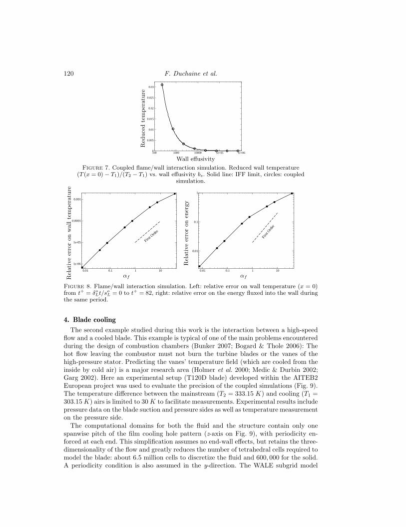
Figure 7 shows how the wall temperature at x = 0 changes when the effusivity ofthe solid varies. For the IFF limit, this temperature is given by Eq. (3.3) and for thesimulation, it is the temperature reached asymptotically for long times. The agreementis excellent and confirms that the IFF limit correctly predicts the long-term evolutionin this FWI problem. It also shows that the coupled simulation works correctly. Note,however, that the IFF limit given by Eq. (3.3) is only approximate for the FWI problemsince it assumes constant density and heat diffusivity in the gases.

Finally, Fig. 8 shows how the coupling frequency (measured by the parameter αf )changes the precision of the coupled simulation (coupling events are scheduled at everyαfτf times where τf is the fluid time). The precision of the coupling was checked bychanging N from 100 to 500, 000 (αf from 7.5 10−3 to 37.8) with Nit = 10 (αf = 7.5 10−4)as reference. The error on the maximum temperature remains very small, even for largeαf values. The error on the maximum energy entering the wall between the initial timeand an arbitrary instant (here δo

Lt/soL = 82) depends strongly on αf . As expected from

results obtained for the IFF problem only (previous section), coupling the two solversless often that τf (αf > 1) leads to errors larger than 10% on the energy fluxed into thewall. The errors on temperature and energy fluxed into the wall converge both to 0 whenαf decreases with an order close to 1.


100 1000 10000 1e+05 1e+060

0.005

0.01

0.015

0.02

0.025

0.03

Wall effusivity

Red

uce

dte

mper

atu

re

Figure 7. Coupled flame/wall interaction simulation. Reduced wall temperature(T (x = 0) − T1)/(T2 − T1) vs. wall effusivity bs. Solid line: IFF limit, circles: coupled

simulation.

0.01 0.1 1 10

1e-06

1e-05

0.0001

0.001

First O

rder

αfRel

ative

erro

ron

wall

tem

per

atu

re

0.01 0.1 1 10

0.01

0.1

1

First

Ord

erαf

Rel

ative

erro

ron

ener

gy

Figure 8. Flame/wall interaction simulation. Left: relative error on wall temperature (x = 0)from t+ = δo

Lt/soL = 0 to t+ = 82, right: relative error on the energy fluxed into the wall during

the same period.

4. Blade cooling

The second example studied during this work is the interaction between a high-speedflow and a cooled blade. This example is typical of one of the main problems encounteredduring the design of combustion chambers (Bunker 2007; Bogard & Thole 2006): Thehot flow leaving the combustor must not burn the turbine blades or the vanes of thehigh-pressure stator. Predicting the vanes’ temperature field (which are cooled from theinside by cold air) is a major research area (Holmer et al. 2000; Medic & Durbin 2002;Garg 2002). Here an experimental setup (T120D blade) developed within the AITEB2European project was used to evaluate the precision of the coupled simulations (Fig. 9).The temperature difference between the mainstream (T2 = 333.15 K) and cooling (T1 =303.15 K) airs is limited to 30 K to facilitate measurements. Experimental results includepressure data on the blade suction and pressure sides as well as temperature measurementon the pressure side.

The computational domains for both the fluid and the structure contain only onespanwise pitch of the film cooling hole pattern (z-axis on Fig. 9), with periodicity en-forced at each end. This simplification assumes no end-wall effects, but retains the three-dimensionality of the flow and greatly reduces the number of tetrahedral cells required tomodel the blade: about 6.5 million cells to discretize the fluid and 600, 000 for the solid.A periodicity condition is also assumed in the y-direction. The WALE subgrid model


Figure 9. Configuration for blade cooling simulation: the T120D blade (AITEB2 project).

Inlet static Inlet total Inlet total Flow Thermal Heat Time Timetemp. temp. pressure rate conduc. cap. scale step ∆tm

f

Mainstream T2(333.15) T t2(339.15) P t

2(27773) 0.0185 2.6 10−2 1015 0.001 9.80 10−8

Cooling air T1(303.15) T t1(303.15) P t

1(29143) 0.000148 2.44 10−2 1015 0.0006 9.80 10−8

Table 3. Flow characteristics for the blade cooling case (SI units). The fluid time scales arebased on the flow-through times in and around the blade. The characteristic fluid time scale τf

is the maximum of this time, i.e., τf = 0.001. The time step ∆tmf is limited by the acoustic CFL

number (0.7).

(Nicoud & Poinsot 1999) is used in conjunction with non-slipping wall conditions. Asshown in Fig. 9, the three film-cooling holes and the plenum are included in the domain:jet 2 is aligned with the main flow (in the xy-plane) while jets 1 and 3 have a com-pound orientation. The mean blowing ratio (ratio of a jet momentum on the hot flowmomentum) of the jets based on a hot gases velocity of 35 ms−1 is approximately 0.4.

Tables 3 and 4 summarize the properties of the gases and of the solid used for the sim-ulation. At each coupling event, fluxes and temperature on the blade skin are exchangedas described in Fig. 1. During this work, only a steady state solution within the solid wassought so that time consistency was not ensured during the coupling computation. Theconverged state is obtained with a two-step methodology:

(a) Initialization of the coupled calculation that includes:• a thermal converged adiabatic fluid simulation,• a thermal converged isothermal solid computation with boundary temperaturesgiven by the fluid solution,

(b) Coupled simulation.Convergence is investigated by plotting the history of the total flux on the blade

(which must go to zero) and of the mean, minimum and maximum blade temperatures.Figures 10 and 11 show these results for two variants of the PCS strategy. In the first


Thermal Heat Density Thermal Time Timeconductivity capacity diffusivity scale τs step

0.184 1450 1190 1.07 10−7 34.22 1.71 10−3

Table 4. Solid characteristics for the blade-cooling case (SI units). The time scale τs iscomputed using the thermal diffusivity and the blade minimum thickness.

0 1 2 3 4 5 6 7 8200

225

250

275

300

325

350

375

400

Reduced time t+ = t/τs

Tem

per

atu

re

0 1 2 3 4 5 6 7 8

0

1

2

3


Tota

lw

all

flux

Figure 10. Time evolution of minimum and maximum temperatures in the blade (left) andtotal heat flux through the blade with (solid) and without (dashed) relaxation.

one, fluxes and temperature are exchanged at each coupling step while for the secondone, relaxation is used and temperature and fluxes imposed at each coupling iteration nare written as fn = afn−1 + (1 − a)fn∗ where fn∗ is the value obtained by the othersolver at iteration n and a is a relaxation factor (typically a = 0.6). Without relaxation,the system becomes unstable and convergence almost impossible.

At the converged state, the total flux reaches zero: the flux entering the blade isevacuated into the cooling air in the plenum and in the holes (Fig. 11). Note howeverthat the analysis of fluxes on the blade skin shows that, even though the blade is heatedby the flow on the pressure side, it is actually cooled on part of the suction side becausethe flow accelerates and cools down on this side. Due to the acceleration in the jets,heat transfer in the holes and plenum are of the same order. Compared to the externalflux, plenum and hole fluxes converge almost linearly. Oscillations in the external fluxevolution are linked with the complex flow structure developing around the blade.

At the converged state, results can be compared to the experiment in terms of pressureprofiles on the blade (on both sides) and of temperature profiles on the pressure side.Pressure fields are displayed in terms of isentropic Mach numbers Mis computed by

Mis =

√

√

√

√

2

γ − 1

[

(

P t2

P tw

)

γ−1

γ

− 1

]

(4.1)

where P t2

and P tw are the total pressure of the mainstream and at the wall. Figure 12

displays an average field of isentropic Mach number obtained by LES and by the ex-periment. The comparison of the adiabatic simulation and the coupled one shows thatthese profiles are only weakly sensitive to the thermal condition imposed on the blade.


0 5 10 15 20 25 30

-0.8

-0.6

-0.4

-0.2

0

0.2

0.4

0.6

0.8


Hea

tfluxes

Figure 11. Time evolution of heat fluxes through the blade: external flux (solid line), plenum(dashed), holes sides (dot), sum of all fluxes (dot dashed).

0 0.2 0.4 0.6 0.8 10

0.2

0.4

0.6

0.8

1

Reduced abscissa

Isen

tropic

Mach

num

ber

Mis

Figure 12. Isentropic Mach number along the blade. Solid line: coupled LES, circles:adiabatic LES, squares: experiment.

Although the shock position on the suction side is not perfectly captured, the overallagreement between LES and experimental results is fair.

Temperature results are displayed in terms of reduced temperature Θ = (T t2−T )/(T t

2−

T t1) where T t

2and T t

1are the total temperatures of the main and cooling streams (Table 4)

and T is the local wall temperature. Θ measures the cooling efficiency of the blade. Fig-ure 13 shows measurements, adiabatic and coupled LES results for Θ spanwise averagedalong axis x. As expected, the cooling efficiency obtained with the adiabatic computa-tion is lower than the experimental values: The adiabatic temperature field over-predictsthe real one. The main contribution of conduction in the blade is to reduce the walltemperature on the pressure side.

The reduced temperature distribution on the pressure side (Fig. 14) shows that thepeak temperature occurs at the stagnation point (reduced abscissa close to 0). The tem-perature at the stagnation point is reduced compared to the adiabatic wall prediction,leading to local values of θ of the order of 0.2. The thermal effects of the cooling jets


0 0.2 0.4 0.6 0.8 10

0.2

0.4

0.6

Reduced abscissa

Cooling

effici

ency

Figure 13. Cooling efficiency Θ versus abscissa on the pressure side at steady state. Dashedline: adiabatic LES, solid line: coupled LES, symbols: experiment, vertical dashed lines: positionof the holes.

Figure 14. Spatial distribution of reduced temperature θ on the pressure side of the blade.The computational domain is duplicated one time in the z-direction.

on the vane are clearly evidenced by Fig. 14. Jet 3 seems to be the most active in thecooling process by protecting the blade from the hot stream until a reduced absissa of0.5 and then impacting the vane between 0.5 and 0.6.

The reduced temperature obtained during this work over-estimates experimental mea-surements. In particular, the strong acceleration caused by the blade induces large ther-mal gradients at the trailing edge. This phenomenon, not-well resolved by the compu-tations, leads to a non-physical values of cooling efficiency. Nevertheless, these resultshave shown great sensitivity to multiple parameters, not only of the coupling strategybut also of the LES models for heat transfer and wall descriptions. Additional studieswill be continued after the Summer Program.

5. Conclusions

Conjugate heat transfer calculations have been performed for two configurations ofimportance for the design of gas turbines with a recently developed massively paralleltool based on a LES solver. (1) An unsteady flame/wall interaction problem was used toassess the precision of coupled solutions when varying the coupling period. It was shownthat the maximum coupling period that allows the temperature and the flux across thewall to reproduce well is of the order of the smallest time scale of the problem. (2)Steady convective heat transfer computation of an experimental film-cooled turbine vaneshowed how thermal conduction in the blade tends to reduce wall temperature comparedto an adiabatic case. Further studies on LES models, coupling strategy and experimental


conditions are needed to improve the quality of the results compared to the experimentalcooling efficiency.

Acknowledgments

The help of L. Pons, from TURBOMECA, and of the AITEB2 consortium regardingaccess to the experimental results is gratefully acknowledged.

REFERENCES

Bogard, D. G. & Thole, K. A. 2006 Gas turbine film cooling. J. Prop. Power 22 (2),249–270.

Buis, S., Piacentini, A. & Declat, D. 2005 PALM: A Computational Frameworkfor assembling High Performance Computing Applications. Concurrency and Com-putation: Practice and Experience .

Bunker, R. S. 2007 Gas turbine heat transfer: Ten remaining hot gas path challenges.Journal of Turbomachinery 129, 193–201.

Chemin, S. 2006 Etude des interactions thermiques fluides-structure par un couplage decodes de calcul. PhD thesis, Universite de Reims Champagne-Ardenne.

Colin, O. & Rudgyard, M. 2000 Development of high-order Taylor-Galerkin schemesfor unsteady calculations. J. Comput. Phys. 162 (2), 338–371.

Dabireau, F., Cuenot, B., Vermorel, O. & Poinsot, T. 2003 Interaction of H2/O2flames with inert walls. Combust. Flame 135 (1-2), 123–133.

Delataillade, A., Dabireau, F., Cuenot, B. & Poinsot, T. 2002 Flame/wallinteraction and maximum heat wall fluxes in diffusion burners. Proc. Combust.Inst. 29, 775–780.

Desoutter, G., Cuenot, B., Habchi, C. & Poinsot, T. 2005 Interaction of apremixed flame with a liquid fuel film on a wall. Proc. Combust. Inst. 30, 259–267.

Ezekoye, O. A., Greif, R. & Lee, D. 1992 Increased surface temperature effectson wall heat transfer during unsteady flame quenching. In 24th Symp. (Int.) onCombustion, pp. 1465–1472. The Combustion Institute, Pittsburgh, Penn.

Garg, V. 2002 Heat transfer research on gas turbine airfoils at NASA GRC. Interna-tional Journal of Heat and Fluid Flow 23 (2), 109–136.

Giles, M. 1997 Stability analysis of numerical interface conditions in fluid-structurethermal analysis. International Journal for Numerical Methods in Fluids 25 (4),421–436.

Holmer, M.-L., Eriksson, L.-E. & Sunden, B. 2000 Heat transfer on a film cooledinlet guide vane. In Proceedings of the ASME Heat Transfer Division, AmericanSociety of Mechanical Engineers , vol. 366-3, pp. 43–50. Orlando, Florida.

Lefebvre, A. H. 1999 Gas Turbines Combustion. Taylor & Francis.

Lu, J. H., Ezekoye, O., Greif, R. & Sawyer, F. 1990 Unsteady heat transfer duringside wall quenching of a laminar flame. In 23rd Symp. (Int.) on Combustion, pp.441–446. The Combustion Institute, Pittsburgh, Penn.

Medic, G. & Durbin, P. A. 2002 Toward improved film cooling prediction. J. Tur-bomach. 124, 193–199.

Mercier, E., Tesse, L. & Savary, N. 2006 3d full predictive thermal chain for gas


turbine. In 25th International Congress of the Aeronautical Sciences . Hamburg, Ger-many.

Moureau, V., Lartigue, G., Sommerer, Y., Angelberger, C., Colin, O. &

Poinsot, T. 2005 High-order methods for DNS and LES of compressible multi-component reacting flows on fixed and moving grids. J. Comput. Phys. 202 (2),710–736.

Nicoud, F. & Poinsot, T. 1999 DNS of a channel flow with variable properties. InInt. Symp. On Turbulence and Shear Flow Phenomena.. Santa Barbara, Calif.

Poinsot, T. & Veynante, D. 2005 Theoretical and numerical combustion. R.T. Ed-wards, 2nd edition.

Popp, P. & Baum, M. 1997 An analysis of wall heat fluxes, reaction mechanisms andunburnt hydrocarbons during the head-on quenching of a laminar methane flame.Combust. Flame 108 (3), 327–348.

Popp, P., Baum, M., Hilka, M. & Poinsot, T. 1996 A numerical study of laminarflame wall interaction with detailed chemistry: wall temperature effects. In Rapportdu Centre de Recherche sur la Combustion Turbulente (ed. T. J. Poinsot, T. Baritaud& M. Baum), pp. 81–123. Rueil Malmaison: Technip.

Roux, A., Gicquel, L. Y. M., Sommerer, Y. & Poinsot, T. J. 2008 Large eddysimulation of mean and oscillating flow in a side-dump ramjet combustor. Combust.Flame 152 (1-2), 154–176.

Schiele, R. & Wittig, S. 2000 Gas turbine heat transfer: Past and future challenges.Journal of Propulsion and Power 16 (4), 583–589.

Schonfeld, T. & Rudgyard, M. 1999 Steady and unsteady flows simulations usingthe hybrid flow solver AVBP. AIAA Journal 37 (11), 1378–1385.

Documents

Center for Turbulence Research Proceedings of the …nicoud/PDF/SP_Duchaine.pdf · Center for Turbulence Research Proceedings of the ... Conjugate heat transfer is a key issue in