Center for Turbulence ResearchProceedings of the Summer Program 2006

57

Numerical investigation and preliminary modelingof a turbulent flow over a multi-perforated plate

By S. Mendez†, J. Eldredge‡, F. Nicoud¶, T. Poinsot‖,M. Shoeybi AND G. Iaccarino

Wall-resolved Large-Eddy Simuations (LES) of a turbulent flow around a multi-perforatedplate are presented. Periodic conditions are used in both directions tangential to the plateso that only one or a few micro-jets are computed. Comparisons between one and fourholes computations show that single-hole domain calculations allow the capture of theessential characteristics and statistics of the flow. The results from two different numer-ical codes and strategies also compare favorably with the existing experimental data inthe case of a large-scale cold flow with effusion. The overall quality of the simulations be-ing established, further analysis of the flow structure is performed. Two results relevantto further modeling studies are obtained: the jet angle somewhat departs from the holeangle, and the velocity profile in the jet is highly inhomogeneous with a strong recircu-lation zone in the downstream side. Preliminary testing of a simple dynamic model forthe normal velocity is also presented. A robust algorithm for implementing this modelin coupled computational domains is developed. Deficiencies in the model are identifiedand discussed.

1. Introduction

In almost all the systems where combustion occurs, solid boundaries need to be cooled.In gas turbines, one often uses multi-perforated walls to produce the necessary cooling(Lefebvre 1999). In this approach, fresh air coming from the casing goes through theperforations and enters the combustion chamber. The associated micro-jets coalesce andproduce a film that protects the internal wall face from the hot gases (Goldstein 1971;Yavuzkurt et al. 1980). The number of submillimetric holes is far too large to allow acomplete description of the generation/coalescence of the jets when computing the 3-Dturbulent reacting flow within the burner. Effusion is however known to have drasticeffects on the whole flow structure, noticeably by changing the flame position. Conse-quently, there is a need to better understand the effects of effusion on the turbulent flowsand to take them into account when performing full-scale Reynolds-Averaged Navier–Stokes (RANS-) or LES-type calculations for design purposes.

Due to technological difficulties, measurements prove highly challenging in the vicinityof multi-perforated plates so that Direct Numerical Simulation (DNS) or wall-resolvedLES are methods of choice to gain insights into the effects of effusion on the turbulentboundary layer. However, the CPU time required for performing such simulations ofa classical case with hundreds of jets would be prohibitive. Two different numericalprocedures were recently proposed and tested (Mendez et al. 2005a,b), the computational

† CERFACS, Toulouse, France‡ Mechanical and Aerospace Engineering Department, University of California, Los Angeles¶ Applied mathematics, University Montpellier II, France - nicoud@math.univ-montp2.fr‖ CNRS IMF Toulouse, France

58 S. Mendez et al.

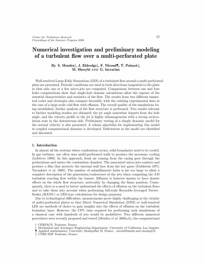
Figure 1. Principle of the large-scale isothermal “LARA” experiment.

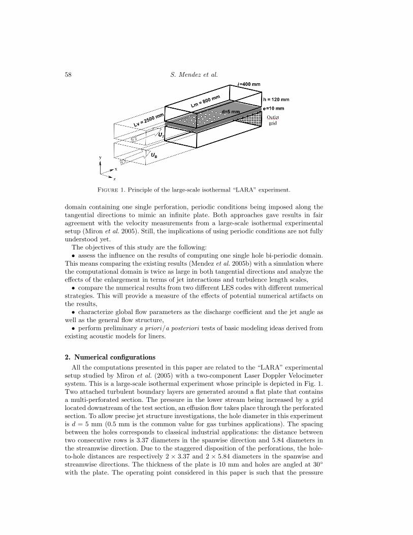
domain containing one single perforation, periodic conditions being imposed along thetangential directions to mimic an infinite plate. Both approaches gave results in fairagreement with the velocity measurements from a large-scale isothermal experimentalsetup (Miron et al. 2005). Still, the implications of using periodic conditions are not fullyunderstood yet.

The objectives of this study are the following:• assess the influence on the results of computing one single hole bi-periodic domain.

This means comparing the existing results (Mendez et al. 2005b) with a simulation wherethe computational domain is twice as large in both tangential directions and analyze theeffects of the enlargement in terms of jet interactions and turbulence length scales,• compare the numerical results from two different LES codes with different numerical

strategies. This will provide a measure of the effects of potential numerical artifacts onthe results,• characterize global flow parameters as the discharge coefficient and the jet angle as

well as the general flow structure,• perform preliminary a priori/a posteriori tests of basic modeling ideas derived from

existing acoustic models for liners.

2. Numerical configurations

All the computations presented in this paper are related to the “LARA” experimentalsetup studied by Miron et al. (2005) with a two-component Laser Doppler Velocimetersystem. This is a large-scale isothermal experiment whose principle is depicted in Fig. 1.Two attached turbulent boundary layers are generated around a flat plate that containsa multi-perforated section. The pressure in the lower stream being increased by a gridlocated downstream of the test section, an effusion flow takes place through the perforatedsection. To allow precise jet structure investigations, the hole diameter in this experimentis d = 5 mm (0.5 mm is the common value for gas turbines applications). The spacingbetween the holes corresponds to classical industrial applications: the distance betweentwo consecutive rows is 3.37 diameters in the spanwise direction and 5.84 diameters inthe streamwise direction. Due to the staggered disposition of the perforations, the hole-to-hole distances are respectively 2 × 3.37 and 2 × 5.84 diameters in the spanwise andstreamwise directions. The thickness of the plate is 10 mm and holes are angled at 30◦

with the plate. The operating point considered in this paper is such that the pressure

Multi-perforated plate 59

COOLING AIR

(b)(a)

WALL

BURNT GASES

DOMAINCALCULATION

FLOWMAIN

INFINITE

MAIN FLOW

WALLPERFORATED

Figure 2. From the infinite plate to the “bi-periodic” calculation domain. (a) Geometry ofthe infinite perforated wall. (b) Calculation domain centered on a perforation; the bold arrowscorrespond to the periodic directions. The distance between two consecutive holes is in the rangeof 6–8 hole diameters.

drop across the plate and blowing ratio (jet-to-“hot” crossflow momentum ratio) are42 Pa and 1.78, respectively. The Reynolds number for the primary “hot” flow (based onthe duct centerline velocity and the half height of the rectangular duct) is Re1 = 17750,while it is Re2 = 8900 for the secondary “cold” flow. The bulk velocity in the “hot”stream is Ub ≈ 4.29 m/s.

2.1. Small-scale computations

In order to gain insight into the detailed structure of the turbulent flow through theliner, it is useful to perform small-scale computations (Mendez et al. 2005b). For thispurpose, the bi-periodic computational domain is designed as the smallest domain thatcan reproduce the geometry of an infinite plate with staggered perforations (Fig. 2). Themain tangential flow at both sides of the plate is enforced by a constant source termadded to the momentum equation, as is usually done in channel flow simulations. Theeffusion flow through the hole is sustained by imposing a uniform vertical mass flow rateat the bottom boundary of the domain. The source terms and uniform vertical mass flowrate were tuned in order to reproduce the operating conditions given in Section 2.

2.2. Large-scale computations

As discussed later in Section 4, a preliminary model for the flow over the liner has beenproposed and implemented in the “CDP” code. Computations of the “LARA” experimentwere performed as a posteriori testing of this liner model. The computational domainfor these calculations is shown in Fig. 3, where the boundary conditions used are alsoshown. Two identical channels share a common wall, part of which is comprised of amulti-perforated liner. Note that in both channels, the computational domain is periodicin the spanwise direction. The mesh contains approximately 106 hexahedra.

3. Numerical results

Two different codes dedicated to LES/DNS in complex geometries have been usedto perform the small-scale simulations, namely the “AVBP” (AVBP 2006) and “CDP”(Ham & Iaccarino 2004) codes. The main characteristics of these codes and associatedsimulations are displayed in Table 1. In this table, < y+ > is an estimate of the averagedfirst off-wall point position in wall units, Vj is the bulk velocity in the hole, and CD

60 S. Mendez et al.

LINER

12 5.4 12

2

4

2

x

y

z

INFLOW 1

INFLOW 2

OUTFLOW 1

OUTFLOW 2

WALLWALL

WALL

WALL

PERIODIC IN z

Figure 3. Large-scale computational domain for the a posteriori testing of the liner model.

Run Code equations Order of mesh < y+ > Vj ∆P CDaccuracy (m/s) (Pa)

AVBP-1H AVBP compressible 3rd 1.5 M tetrahedra 5 5.6 41 0.66

CDP-1H CDP incompressible 2nd 1.5 M hexahedra 1 5.6 39.5 0.67

AVBP-4H AVBP compressible 3rd 6 M tetrahedra 5 5.6 41 0.66

Table 1. Main characteristics of the small-scale simulations

is the discharge coefficient Vj/√

2∆p/ρ. Two kinds of comparisons are discussed in thefollowing subsections:• AVBP-1H/AVBP-4H comparison: for a given numerical methodology, two simula-

tions with different computational domain sizes are compared in Section 3.1 in order toestablish the validity of the one-hole based simulations,• AVBP-1H/CDP-1H comparison: for a given computational domain and operating

point, two simulations performed with two different implementations of the Navier-Stokesequations are compared in Section 3.2 in order to establish that the computed fields arenot contaminated by numerical errors.

3.1. Effect of the number of holes

By making use of a bi-periodic computational domain containing a single hole, one forcesthe hole-to-hole distance to play a major role in the simulation. Any turbulence lengthscale greater than half the domain size would not have enough room to appear and, moreimportantly, jet-to-jet interaction cannot take place. Given that the jet-to-jet distanceis only 6–10 hole diameters, basing the study on one-hole bi-periodic computations is aquestionable choice. The purpose of this section is to assess how the results are modified,if they are, by this arbitrary choice. To this end, a LES of a bi-periodic computationaldomain twice as large in each tangential direction has been performed with the AVBPcode (Run AVBP-4H in Table 1). The mesh is the same as for the 1-hole computation(Run AVBP-1H in Table 1), duplicated four times. In order to save CPU time, the initialcondition for this 4-hole computation is a four-times duplicated version of an establishedsolution from the 1-hole simulation. Figure 4 shows the time evolution of the streamwisevelocity at four sensors located 1 diameter above each of the four computed holes. Asexpected, they initially behave similarly and after approximately two flow-through times(FTT), the instantaneous evolutions become different from one jet to the other. Note that

Multi-perforated plate 61

1.2

1.1

1.0

0.9

0.8

3.02.52.01.51.00.50.0

PSfrag replacements

time (FTT)

<U>/Vj

1.2

1.1

1.0

0.9

0.8

13.012.011.010.0

PSfrag replacements

time (FTT)< U > /Vj

time (FTT)

<U>/Vj

Figure 4. Time evolution of the streamwise velocity one diameter above the four holes in the“hot” stream. Left: beginning of the run, Right: after the transitional phase.

Figure 5. Instantaneous iso-surface of velocity modulus (1.125 Vj) colored by the normalvelocity component (scale is from −0.18 Vj (black) to 0.71 Vj (white)) for the AVBP-4H run.

the FTT is based on the jet-to-jet streamwise distance and bulk velocity in the primaryflow, while the length and velocity scales chosen for most of the plots in the paper arethe hole diameter d and hole bulk velocity Vj . The statistics discussed in the remainderof this section have been obtained over 10 FTT, while the accumulation process startedat 13 FTT. It is assumed that any jet-to-jet interaction would have had enough time toappear during the total of 23 FTT that were computed. Since a detailed analysis of thesnapshots over the simulation showed no such event, it is believed that the micro-jets arenot subject to collective interaction, at least for the operating point considered in thisstudy.

A typical snapshot of a velocity iso-surface is depicted in Fig. 5, which shows that thefour jets do not have the same appearance. Some seem very quiescent, with a laminar typeof velocity iso-surface, others are characterized by an intense vortex- shedding process(see the most downstream and the most upstream jets in Fig. 5), while the foregroundjet shows an intermediate behavior. Note that these two types of states can be foundalternatively in any of the computed jets, which is expected since they are all statisticallyequivalent. The same intermittent behavior is found in the 1-hole simulation as shown inFig. 6, which displays the same iso-velocity surface at different times over the simulation.

In terms of statistics, the 1-hole and 4-hole configurations also lead to very similarresults. This is illustrated in Figs. 7 and 8, where the profiles of the averaged and rootmean square (rms) of the streamwise and normal velocity components are shown for twolocations downstream of the hole. In these plots the profiles corresponding to the fourholes of the 4-hole computation are represented by the same line type since there is no

62 S. Mendez et al.

Figure 6. Instantaneous iso-surface of velocity modulus (1.125 Vj) colored by the normal ve-locity component (scale is from −0.18 Vj (white) to 0.71 Vj (black)) for the AVBP-1H run attwo different instants.

12

10

8

6

4

2

0

1.20.80.40.0

PSfrag replacements

< U > /Vj

y/D

(a)12

10

8

6

4

2

0

0.300.200.100.00

PSfrag replacements

< U > /Vjy/D

(a)

< V > /Vj

y/D

(b)

12

10

8

6

4

2

0

0.250.200.150.100.050.00

PSfrag replacements

< U > /Vjy/D

(a)< V > /Vj

y/D(b)

urms/Vj

y/D

(c)12

10

8

6

4

2

0

0.150.100.050.00

PSfrag replacements

< U > /Vjy/D

(a)< V > /Vj

y/D(b)

urms/Vjy/D

(c)

vrms/Vj

y/D

(d)

Figure 7. Velocity profiles from the AVBP-1H ( ) and AVBP-4H ( ) computations2.92 diameters downstream of the hole: (a) time averaged streamwise velocity, (b) time averagednormal velocity, (c) rms of streamwise velocity, (d) rms of normal velocity.

statistical difference between these profiles. The differences observed are due to the lackof statistical convergence and provide an easy way to estimate the statistical incertitudein the plotted profiles. Given this error bound, there is no difference between the 1-holeand the 4-hole computations. The same conclusion was drawn from all the one-pointstatistics comparisons performed between the two configurations.

Typical streamwise two-point correlations are depicted in Fig. 9 for the streamwiseand normal velocity. These profiles were obtained by post-processing 25 independentsolutions of AVBP-4H and 62 AVBP-1H snapshots. The four-hole regions in AVBP-4Hwere subsequently averaged together to obtain the results shown in this figure, whichalso depicts the position of the reference points for the computation of the streamwisetwo-point correlations. In one case (Figs. 9a, c) the reference point (which correspondsto zero axial distance in the figure) is located above a hole and the end point is lo-cated above the next hole in the downstream direction. In the other case (Figs. 9b, d),the reference point is located at half distance between two consecutive lines of holes.In general, no major difference is present between AVBP-1H and AVBP-4H, supportingthe fact that no major artifacts are present in the 1-hole simulation. Note however that

Multi-perforated plate 63

12

10

8

6

4

2

0

1.00.80.60.40.20.0

PSfrag replacements

< U > /Vj

y/D

(a)12

10

8

6

4

2

0

0.200.150.100.050.00

PSfrag replacements

< U > /Vjy/D

(a)

< V > /Vj

y/D

(b)

12

10

8

6

4

2

0

0.160.120.080.040.00

PSfrag replacements

< U > /Vjy/D

(a)< V > /Vj

y/D(b)

urms/Vj

y/D

(c)12

10

8

6

4

2

0

0.160.120.080.040.00

PSfrag replacements

< U > /Vjy/D

(a)< V > /Vj

y/D(b)

urms/Vjy/D

(c)

vrms/Vj

y/D

(d)

Figure 8. Velocity profiles from the AVBP-1H ( ) and AVBP-4H ( ) computations5.84 diameters downstream of the hole (viz. in between two consecutive holes in the spanwise orstreamwise direction): (a) time averaged streamwise velocity, (b) time averaged normal velocity,(c) rms of streamwise velocity, (d) rms of normal velocity.

non-negligible differences between AVBP-1H and AVBP-4H are present for the normalvelocity two-point correlation (Fig. 9c). Given the very good agreement observed previ-ously for instantaneous velocity (Figs. 5 and 6) and for the mean and rms of streamwiseand normal velocities (Figs. 7 and 8), this difference is most likely due to a lack of sta-tistical convergence. From a physical perspective, Fig. 9 also suggests that the micro-jetshave a strong effect on the turbulence structure. Indeed, the integral turbulence lengthscale Luu assessed from Fig. 9a, viz. along a line crossing the micro-jets is about twicesmaller than what is obtained from Fig. 9b, viz. along a line where jets are not present.With a streamwise hole-to-hole distance of 11.68 d, the two assessments of Lx are roughly1.2 and 2.4 hole diameters. The same trend is observed from plots 9c and 9d.

3.2. Cross-code comparison and flow structure

As mentioned in Table 1, the discharge coefficient from the two 1-hole simulations fromthe two codes AVBP and CDP are very close, of order 0.66. Besides this agreement inthe global parameter CD, the two codes predict very similar jet structure. In both cases,the jet separates at the entry of the hole (Fig. 10, left column) and two different regionscan be defined: the jetting region, near the upstream wall of the hole, where the jetshows high velocities, and the low-momentum region close to the downstream boundaryof the hole. Note that because of the entrainment by the outer stream, the jet angle atthe aperture outlet is somewhat different from the geometrical angle: it is approximately28◦, while the angle of the hole is 30◦. As the length of the holes is small, the jet atthe exit of the hole is still highly influenced by what happens at the entry of the hole.Figure 10 (right column) also shows that two counter-rotating vortices are present in thehole itself. Local asymmetries in the velocity field of the AVBP simulation are attributedto probable statistical convergence. The direction of rotation of these vortices is the sameas for the classical counter-rotating vortex pair that is observed in jets in crossflow studies(see Andreopoulos & Rodi (1984)).

64 S. Mendez et al.

-1.0

-0.5

0.0

0.5

1.0

1.00.80.60.40.20.0

PSfrag replacements

Streamwise distance

Cuu

(a)

-1.0

-0.5

0.0

0.5

1.0

1.00.80.60.40.20.0

PSfrag replacements

Streamwise distanceCuu

(a)

Streamwise distance

Cuu

(b)

FLOWMEAN

10

10

PSfrag replacements

Streamwise distanceCuu

(a)

Streamwise distanceCuu

(b)I

II

-1.0

-0.5

0.0

0.5

1.0

1.00.80.60.40.20.0

PSfrag replacements

Streamwise distanceCuu

(a)

Streamwise distanceCuu

(b)

III

Streamwise distance

Cvv

(c)

-1.0

-0.5

0.0

0.5

1.0

1.00.80.60.40.20.0

PSfrag replacements

Streamwise distanceCuu

(a)

Streamwise distanceCuu

(b)

III

Streamwise distanceCvv

(c)

Streamwise distance

Cvv

(d)

Figure 9. Streamwise two-point correlation coefficients for the streamwise [plots (a) and (b)]and normal [plots (c) and (d)] velocity from AVBP-1H ( ) and AVBP-4H ( ) at 1.2diameter above the liner for paths I [plots (a) and (c)] and II [plots (b) and (d)]. The sketchbetween the plots depicts the paths along which the correlations have been computed.

Figure 10. Computed mean streamwise velocity in the hole region. Top row: AVBP-1H, Bottomrow: CDP-1H, Left column: Centerline plane, Right column: plane perpendicular to the jet flow(see white line in the left column). Scale is from −0.18 Vj (white) to 1.24 Vj (black).

Multi-perforated plate 65

12

10

8

6

4

2

0

1.21.00.80.60.40.20.0

PSfrag replacements

< U > /Vj

y/D

(a)12

10

8

6

4

2

0

0.300.200.100.00

PSfrag replacements

< U > /Vjy/D

(a)

< V > /Vj

y/D

(b)

12

10

8

6

4

2

0

0.250.200.150.100.050.00

PSfrag replacements

< U > /Vjy/D

(a)< V > /Vj

y/D(b)

urms/Vj

y/D

(c)12

10

8

6

4

2

0

0.200.150.100.050.00

PSfrag replacements

< U > /Vjy/D

(a)< V > /Vj

y/D(b)

urms/Vjy/D

(c)

vrms/Vj

y/D

(d)

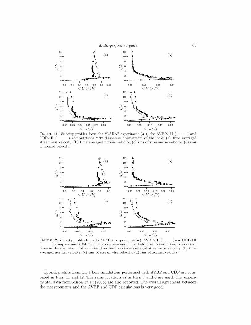
Figure 11. Velocity profiles from the “LARA” experiment (• ), the AVBP-1H ( ) andCDP-1H ( ) computations 2.92 diameters downstream of the hole: (a) time averagedstreamwise velocity, (b) time averaged normal velocity, (c) rms of streamwise velocity, (d) rmsof normal velocity.

12

10

8

6

4

2

0

1.00.80.60.40.20.0

PSfrag replacements

< U > /Vj

y/D

(a)12

10

8

6

4

2

0

0.250.200.150.100.050.00

PSfrag replacements

< U > /Vjy/D

(a)

< V > /Vj

y/D

(b)

12

10

8

6

4

2

0

0.150.100.050.00

PSfrag replacements

< U > /Vjy/D

(a)< V > /Vj

y/D(b)

urms/Vj

y/D

(c)12

10

8

6

4

2

0

0.150.100.050.00

PSfrag replacements

< U > /Vjy/D

(a)< V > /Vj

y/D(b)

urms/Vjy/D

(c)

vrms/Vj

y/D

(d)

Figure 12. Velocity profiles from the “LARA” experiment (• ), AVBP-1H ( ) and CDP-1H( ) computations 5.84 diameters downstream of the hole (viz. between two consecutiveholes in the spanwise or streamwise direction): (a) time averaged streamwise velocity, (b) timeaveraged normal velocity, (c) rms of streamwise velocity, (d) rms of normal velocity.

Typical profiles from the 1-hole simulations performed with AVBP and CDP are com-pared in Figs. 11 and 12. The same locations as in Figs. 7 and 8 are used. The experi-mental data from Miron et al. (2005) are also reported. The overall agreement betweenthe measurements and the AVBP and CDP calculations is very good.

66 S. Mendez et al.

4. Preliminary liner modeling

The ultimate goal of this ongoing work is to develop an equivalent model for thebehavior of a multi-perfortated liner in turbulent flow. This model should, ideally, providean accurate description of the mean flow and turbulence statistics of the coalesced filmproduced by the array of jets issuing from the holes in the liner. In this section we proposea simple model for the behavior of a multi-perforated liner and describe its numericalimplementation. We present results from simulation of the coupled flow through parallelrectangular channels that communicate via the liner, in the configuration used in the“LARA” experiments.

4.1. Formulation

The present liner model is based on a simple description of the unsteady high Reynoldsnumber flow through a circular aperture proposed by Howe (1979). This previous workwas motivated by an interest in the interaction of acoustic waves with an aperture with amean bias flow. However, the aperture model itself is incompressible, as the velocities inthe vicinity of the aperture are generally small compared with the mean speed of sound.Howe obtained a linear relation between the fluctuating volume flow rate through thehole and the pressure fluctuations across it by hypothesizing an unsteady vortex sheetshed from the aperture rim. These vorticity fluctuations act as an acoustic sink andare convected away by the mean bias flow. Eldredge and Dowling (2003) developed ahomogeneous liner acoustic impedance from this aperture model by smearing the meanaperture flow about the cell that encloses it. They found very good agreement betweenthe model and isothermal acoustic experiments.

The success of the linear model in acoustic experiments demonstrates that it can suc-cessfully relate fluctuations in the through-flow of the liner to small pressure fluctuationsin its vicinity. Furthermore, the basic principle of the model should also hold, even whenthese fluctuations are large. It has recently been shown by Luong et al. (2005) that themodel is consistent with a non-linear model developed by Cummings (1983). The non-linear Cummings model, when specialized to cases in which the aperture flow does notreverse, is written as

l′∂Uh∂t

+1

2σ2U2h =

1

ρ∆p, (4.1)

where Uh is the spatially average velocity through the aperture and ∆p is the pressuredrop across the aperture. The constant parameters in the model are σ, the contractioncoefficient of the issuing jet, and l′, a length scale that accounts for the inertia of fluid inand around the aperture. From consideration of the added mass of fluid adjacent to theaperture entrance and exit, then l′ = lw + π

2 a, where lw is the physical thickness of theliner and a is the aperture radius. Physically, the second term in Eq. 4.1 describes theloss of dynamic pressure as the jet emerges from the hole and mixes with the surroundingfluid. The unsteady term introduces a time lag due to fluid inertia.

These observations suggest that the model is a worthy candidate for describing amulti-perforated liner in turbulence simulations. We can follow a similar approach toEldredge and Dowling (2003) to extend the aperture model (4.1) to a homogeneousliner. We suppose that the local normal velocity, uN , is spatially distributed over the cellsurrounding an aperture, so that

uN = αUh, (4.2)

where α is the porosity of the liner (defined as the total open area divided by the total

Multi-perforated plate 67

area of the liner). By conservation of mass, this through-flow velocity provides a Dirichletcondition for the flows on either side of the liner; in this case, the no-slip condition isenforced.

The interface model embodied in Eq. 4.2 gives no consideration to tilting of the aper-tures, nor the associated streamwise momentum that the discrete jets inject into theflow. These features are responsible for the film structure created by the coalescing jets.We therefore also propose a slightly more sophisticated model for both the normal andstreamwise tangential velocity components,

uN = αUh sinφ, (4.3)

uT = Uh cosφ, (4.4)

for apertures of angle φ (where φ = π/2 with no tilting). Note that the porosity isnot used in the slip velocity component. The streamwise momentum flux in the jet isapproximately ρU2

hAh cosφ sinφ, where Ah is the cross-sectional area of the hole. Fromthe modeled liner, the flux is ρuNuTAc distributed over a cell of area Ac = Ah/α.Relations 4.3 and 4.4 ensure that both mass and streamwise momentum flux from thehomogeneous liner are equivalent to the discrete jets. In this model, we only enforce theslip velocity in Eq. 4.4 on the exit side of the liner; the no-slip condition is still enforcedon the entrance side. This choice can be explored in future work. In the next section, wedescribe the implementation of this model in a full numerical simulation.

4.2. Implementation

The numerical implementation described here is focused specifically on a control volume-based collocated fractional-step method for computing incompressible flows on unstruc-tured grids (Mahesh et al. 2004). However, its implementation can be generalized to othermethodologies. There are two essential aspects of this implementation: stable integrationof the aperture velocity model (4.1) and coupling of the two computational domains viathis model.

Consistent with the interior scheme, we integrate Eq. 4.1 with a fractional step method:

Uh − Unh∆t

= − 1

2σ2l′U2h +

1

ρ

∆pn−1/2

l′, (4.5a)

U∗h − Uh∆t

= −1

ρ

∆pn−1/2

l′, (4.5b)

Un+1h − U∗h

∆t=

1

ρ

∆pn+1/2

l′. (4.5c)

Though this model nominally involves the “aperture velocity”, the equations are treatedas spatially continuous, and Uh merely serves as an intermediate variable for the normaland tangential velocity components.

The pressure differences in this model require careful consideration. We take ∆p to bethe difference in pressures immediately adjacent to each side of the liner, ∆p = p2 − p1,where the subscripts refer to the computational domains, and uN is defined as positivewhen directed from 2 to 1. In the first substep, the pressures from the previous time stepare used to advance the liner normal velocity. The intermediate liner velocity uN is easilyfound as the sole physical root of the quadratic Eq. 4.5a. This velocity is enforced as aDirichlet boundary condition (along with no-slip conditions in the tangent components)during the advancement of the first fractional step of the interior momentum equations.

68 S. Mendez et al.

Conservation of mass requires that the final substep (4.5c) must be considered inconjunction with the pressure Poisson equation formed from the corresponding substepin the interior. For any face adjoining two control volumes, the face-normal velocitycomponent, Uf , obeys the following equation in the last substep:

Un+1f − U∗f

∆t= −1

ρ

∂p

∂n

n+1/2

, (4.6)

where n is directed out of the volume. Local conservation of mass requires that the sumof the fluxes through the faces of each control volume must vanish at the end of the step.For interior control volumes, this leads to the following relation:

∑

f

∂p

∂n

n+1/2

Af =ρ

∆t

∑

f

U∗fAf . (4.7)

However, the flux through the face on the liner is determined by Eq. 4.5c with either 4.2or 4.3. Thus the overall pressure Poisson system is modified for control volumes alongthe liner. For example, for liner-adjacent control volumes in domain 1, using Eq. 4.3 todetermine the normal velocity, we arrive at:

∑

f ′

∂p

∂n

n+1/2

Af − α sinφpn+1/21

l′Af =

ρ

∆t

∑

f ′

U∗fAf − u∗NAf

− α sinφ

pn+1/22

l′Af ,

(4.8)where the sums are only taken over the interior faces.

Clearly, the pressure Poisson systems are coupled for domains 1 and 2 by the inter-face equations (4.8). To avoid having to solve these systems simultaneously, we utilize astaggered time approach:

(a) For both domains, Unh is used to provide the current interface conditions.

(b) The pressure difference in the final substep is defined as ∆pn+1/2 = pn−1/22 −pn+1/2

1 .

The Poisson system in domain 1 is solved using the modified Eq. (4.8) with pn−1/22 , and

Un+1h is derived from the result using (4.5c).(c) Simultaneously, the Poisson system in domain 2 is solved with no modification.(d) At the end of these steps, the wall-normal velocity from domain 1 is exchanged

with domain 2, and the liner pressure in domain 2 is exchanged with domain 1.This approach ensures minimal latency of the parallel computations in each domain.

Note that this algorithm can be iteratively corrected, with the last three steps alternatedbetween the domains. However, the error after only a single iteration is of order ∆t,which is consistent with the remainder of the fractional step methodology.

4.3. A priori evaluation of model

An initial evaluation of the liner model is presented in this section. Three hundred fieldsfrom the AVBP-1H run have been post-processed in order to compute the three termsof Eq. 4.1. Given the geometric characteristics of the perforated plate, the l′ length scaleequals 23 mm while the contraction coefficient is considered to be equal to the dischargecoefficient obtained in AVBP : σ = CD = 0.66 (Table 1). The first idea was to computethe pressure drop ∆p in two different ways: as the difference between the mean pressureat the hole inlet and outlet (∆ph), or as the difference between the mean pressure overthe computational domain inlet and outlet (∆p∞). However, two reasons indicate that∆p∞ is a better candidate than ∆ph to test the model of Eq. 4.1.

Multi-perforated plate 69

PSfrag replacements

(a)

1.19

1.18

1.17

1.16

1.15

43210

PSfrag replacements

(a)

time (FTT)

(b)

Figure 13. The liner model: a priori test from the AVBP-1H run (a): Average pressure field onthe centerline plane. (b): Time evolution of the pressure drop post-processed from the AVBP-1H

run: ∆P∞ ( ). Comparison with the pressure drop from Eq. 4.1, viz. ρl′ ∂Uh∂t

+ ρ2σ2U

2h

( ) and with the pressure drop from Eq. 4.1 without the unsteady term, viz. ρ2σ2U

2h

( ). All terms scaled by ρV 2j .

• The model proposed by Howe (1979) is based on variations of the external pressurefar from the aperture, more represented by ∆p∞.• Figure 13a shows the pressure field on the centerline plane: at the hole inlet, the

pressure is inhomogeneous: it varies from the far field pressure in the “cold” side P2 to thefar field pressure in the “hot” side P1 in a very small region (see the circle in Fig. 13a).

The averaged velocity in the hole Uh has been computed over a plane situated at halfthe thickness of the plate (shown by the horizontal line in Fig. 13a). In order to test theliner model, the pressure drop reconstructed from the Uh signal by using Eq. 4.1 can becompared with the pressure drop directly computed from the AVBP-1H run.

The comparison is shown in Fig. 13b, which demonstrates that on the average, ∆p∞is well reproduced by the liner model (Eq. 4.1), even if the pressure fluctuations areoverestimated. Still, the error between the pressure drop measured in the calculation andthe one reconstructed from Uh is never bigger than 4%. The term related to the inertiaof the fluid introduces fluctuations in high frequencies but does not improve the model.Indeed the inertia of the fluid contained in the hole is not a first-order term in the linermodel. Note that one can expect that these results would not hold if strong acousticwaves were impinging the liner.

4.4. A posteriori evaluation of model

In this section, we present the results of numerical simulations of a turbulent flow throughparallel rectangular channels. A finite section of the common wall between the channels iscomposed of a multi-perforated liner, as can be seen in Fig. 3. In terms of the half-heightof the channel, h, the width of the channel is 4h, the entry length upstream of the liner is12h, and the length of the liner is 5.4h. The liner extends across the entire width of thechannel. These proportions are equivalent to the experiments conducted on the “LARA”test rig. The computational domain extends a further 12h units downstream of the endof the liner.

The simulations are conducted at centerline Reynolds number of 4000 and 2000 in theupper and lower channels, respectively. Note that these Reynolds numbers are approx-imately 4.5 times smaller than those used in the “LARA” experiments, and are chosento ensure computational economy in this initial evaluation. A constant value is addedto the pressure in the lower channel so that the mean pressure drop across the lineris 42 Pa. Periodic boundary conditions are used in the spanwise direction to suppressnon-physical behavior at the junction between the liner and vertical side walls. The in-let velocity profiles in both channels are eighth-degree polynomials, randomly perturbed

70 S. Mendez et al.

00 0.4 -0.04 0 0.04 0.080.8 1.2

1

0.8

0.6

0.4

0.2

0

1

0.8

0.6

0.4

0.2

<V>/Uc<U>/Uc

y/h

y/h

(a) (b)

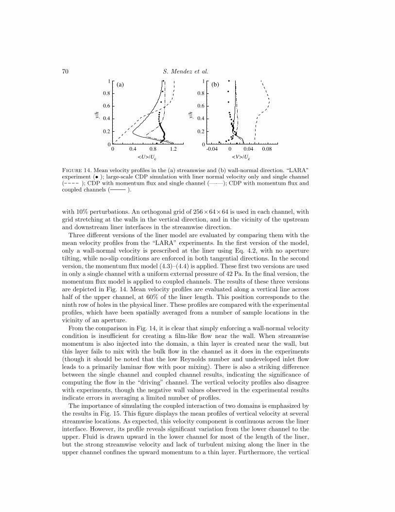
Figure 14. Mean velocity profiles in the (a) streamwise and (b) wall-normal direction. “LARA”experiment (• ); large-scale CDP simulation with liner normal velocity only and single channel( ); CDP with momentum flux and single channel (—·—); CDP with momentum flux andcoupled channels ( ).

with 10% perturbations. An orthogonal grid of 256×64×64 is used in each channel, withgrid stretching at the walls in the vertical direction, and in the vicinity of the upstreamand downstream liner interfaces in the streamwise direction.

Three different versions of the liner model are evaluated by comparing them with themean velocity profiles from the “LARA” experiments. In the first version of the model,only a wall-normal velocity is prescribed at the liner using Eq. 4.2, with no aperturetilting, while no-slip conditions are enforced in both tangential directions. In the secondversion, the momentum flux model (4.3)–(4.4) is applied. These first two versions are usedin only a single channel with a uniform external pressure of 42 Pa. In the final version, themomentum flux model is applied to coupled channels. The results of these three versionsare depicted in Fig. 14. Mean velocity profiles are evaluated along a vertical line acrosshalf of the upper channel, at 60% of the liner length. This position corresponds to theninth row of holes in the physical liner. These profiles are compared with the experimentalprofiles, which have been spatially averaged from a number of sample locations in thevicinity of an aperture.

From the comparison in Fig. 14, it is clear that simply enforcing a wall-normal velocitycondition is insufficient for creating a film-like flow near the wall. When streamwisemomentum is also injected into the domain, a thin layer is created near the wall, butthis layer fails to mix with the bulk flow in the channel as it does in the experiments(though it should be noted that the low Reynolds number and undeveloped inlet flowleads to a primarily laminar flow with poor mixing). There is also a striking differencebetween the single channel and coupled channel results, indicating the significance ofcomputing the flow in the “driving” channel. The vertical velocity profiles also disagreewith experiments, though the negative wall values observed in the experimental resultsindicate errors in averaging a limited number of profiles.

The importance of simulating the coupled interaction of two domains is emphasized bythe results in Fig. 15. This figure displays the mean profiles of vertical velocity at severalstreamwise locations. As expected, this velocity component is continuous across the linerinterface. However, its profile reveals significant variation from the lower channel to theupper. Fluid is drawn upward in the lower channel for most of the length of the liner,but the strong streamwise velocity and lack of turbulent mixing along the liner in theupper channel confines the upward momentum to a thin layer. Furthermore, the vertical

Multi-perforated plate 71

x/h=11 12 13 14 15 16 17

2

1

0

-1

-2

0 0.02-0.02<V>/U

c

y/h

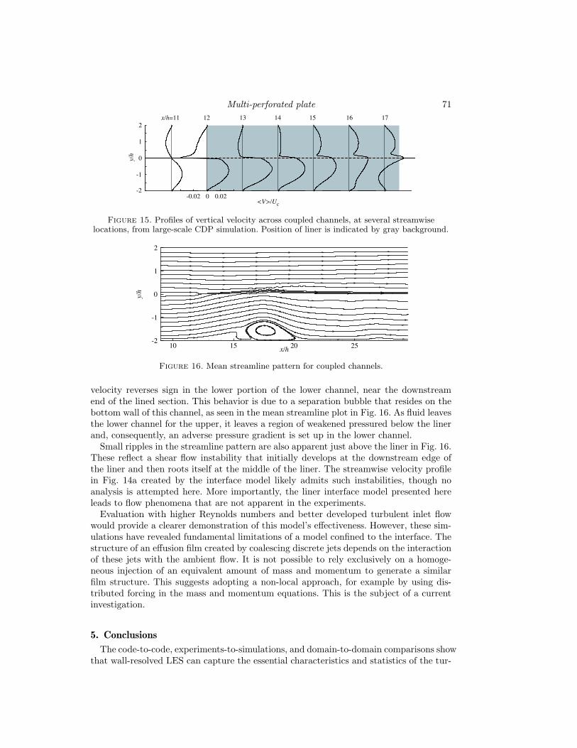
Figure 15. Profiles of vertical velocity across coupled channels, at several streamwiselocations, from large-scale CDP simulation. Position of liner is indicated by gray background.

x/h

y/h

10 15 20 25-2

-1

0

1

2

Figure 16. Mean streamline pattern for coupled channels.

velocity reverses sign in the lower portion of the lower channel, near the downstreamend of the lined section. This behavior is due to a separation bubble that resides on thebottom wall of this channel, as seen in the mean streamline plot in Fig. 16. As fluid leavesthe lower channel for the upper, it leaves a region of weakened pressured below the linerand, consequently, an adverse pressure gradient is set up in the lower channel.

Small ripples in the streamline pattern are also apparent just above the liner in Fig. 16.These reflect a shear flow instability that initially develops at the downstream edge ofthe liner and then roots itself at the middle of the liner. The streamwise velocity profilein Fig. 14a created by the interface model likely admits such instabilities, though noanalysis is attempted here. More importantly, the liner interface model presented hereleads to flow phenomena that are not apparent in the experiments.

Evaluation with higher Reynolds numbers and better developed turbulent inlet flowwould provide a clearer demonstration of this model’s effectiveness. However, these sim-ulations have revealed fundamental limitations of a model confined to the interface. Thestructure of an effusion film created by coalescing discrete jets depends on the interactionof these jets with the ambient flow. It is not possible to rely exclusively on a homoge-neous injection of an equivalent amount of mass and momentum to generate a similarfilm structure. This suggests adopting a non-local approach, for example by using dis-tributed forcing in the mass and momentum equations. This is the subject of a currentinvestigation.

5. Conclusions

The code-to-code, experiments-to-simulations, and domain-to-domain comparisons showthat wall-resolved LES can capture the essential characteristics and statistics of the tur-

72 S. Mendez et al.

bulent flow with effusion. The related computing effort can be reduced significantly byusing a single-hole bi-periodic computational domain since jet-to-jet interaction does notseem to occur, at least for the operating points considered. This opens new perspectivesin terms of generating relevant data for supporting the development of wall models rele-vant to effusion cooling applications. A preliminary model for the multi-perforated linerhas been presented, and a posteriori testing has been conducted with the configurationof the “LARA” experimental rig. A robust algorithm has been developed to integrate thedynamic model in a mass-conservative manner, and to efficiently couple the computa-tional domains that share the liner at their interface. The results reveal that the model isinsufficient for providing the equivalent structure of an effusion film produced by discretejets. A more sophisticated approach will be pursued in future work.

Acknowledgments

The authors gratefully acknowledge support from CINES for the computer resourcesand the European Community for participating in the funding of this work under theproject INTELLECT-DM (Contract No. FP6 - AST3 - CT - 2003 - 502961).

REFERENCES

Andreopoulos, J. & Rodi, W. 1984 Experimental investigation of jets in a crossflow.J. Fluid Mech. 138, 93–127.

AVBP 2006 AVBP Code: www.cerfacs.fr/cfd/avbp code.php andwww.cerfacs.fr/cfd/CFDPublications.html

Cummings, A. 1983 Acoustic nonlinearities and power losses at orifices. AIAA J. 22 (6),786–792.

Eldredge, J. D. & Dowling, A. P. 2003 The absorption of axial acoustic waves bya perforated liner with bias flow. J. Fluid Mech. 485, 307–335.

Goldstein, R. J. 1971 Film Cooling. In Adv. Heat Transfer 7, 321–379 . Ed. AcademicPress, New York and London.

Ham, F. & Iaccarino, G. 2004 Energy conservation in collocated discretizationschemes on unstructured meshes. In Annual Research Briefs 2004, Center for Tur-bulence Research, NASA Ames/Stanford Univ.

Howe, M. S. 1979 On the theory of unsteady high Reynolds number flow through acircular aperture. Proc. Roy. Soc. Lond. A 366, 205-223.

Lefebvre, A. H. 1999 Gas Turbines Combustion. Taylor & Francis.

Luong, T., Howe, M. S. & McGowan, R. S. 2005 On the Rayleigh conductivity ofa bias-flow aperture. J. Fluid Struct. 21, 769–778.

Mahesh, K., Constantinescu, G. & Moin, P. 2004 A numerical method for Large-eddy simulation in complex geometries. J. Comp. Phys. 197, 215-240. CTR04.

Mendez, S., Nicoud, F. & Miron, P. 2005a Direct and large eddy simulations of aturbulent flow with effusion. In ERCOFTAC Workshop - DLES6. Poitiers, France.

Mendez, S., Nicoud, F. & Poinsot, T. 2005b Large-eddy simulation of a turbulentflow around a multi-perforated plate. In CY-LES. Limassol, Cyprus.

Miron, P., Mendez, S., Nicoud, F. & Berat, C. 2005 Comparison between lda mea-surements and LES predictions of cold airflows through a multi-perforated plate. InNumerical Heat Transfer 2005 EUROTHERM Seminar 82. Gliwice-Cracow, Poland.

Yavuzkurt, S., Moffat, R. J. & Kays, W. M. 1980 Full coverage film cooling. Part1. Three-dimensional measurements of turbulence structure. J. Fluid Mech. 101,129–158.