arX

iv:1

411.

4863

v1 [

cond

-mat

.mtr

l-sc

i] 1

8 N

ov 2

014

Spin transfer torques generated by the anomalous Hall effect and anisotropic

magnetoresistance.

Tomohiro TaniguchiNational Institute of Advanced Industrial Science and Technology (AIST),

Spintronics Research Center, Tsukuba, Ibaraki 305-8568, Japan andCenter for Nanoscale Science and Technology, National Institute of

Standards and Technology, Gaithersburg, Maryland 20899-6202, USA

J. GrollierUnite Mixte de Physique CNRS/Thales and Universite Paris Sud 11, 1 Avenue Fresnel, 91767 Palaiseau, France

M. D. StilesCenter for Nanoscale Science and Technology, National Institute of

Standards and Technology, Gaithersburg, Maryland 20899-6202, USA

Spin-orbit coupling in ferromagnets gives rise to the anomalous Hall effect and the anisotropicmagnetoresistance, both of which can be used to create spin-transfer torques in a similar manneras the spin Hall effect. In this paper we show how these effects can be used to reliably switchperpendicularly magnetized layers and to move domain walls. A drift-diffusion treatment of theanomalous Hall effect and the anisotropic magnetoresistance describes the spin currents that flowin directions perpendicular to the electric field. In systems with two ferromagnetic layers separatedby a spacer layer, an in-plane electric field cause spin currents to be injected from one layer into theother, creating spin transfer torques. Unlike the related spin Hall effect in non-magnetic materials,the anomalous Hall effect and the anisotropic magnetoresistance allow control of the orientation ofthe injected spins, and hence torques, by changing the direction of the magnetization in the injectinglayer. The torques on one layer show a rich angular dependence as a function of the orientation of themagnetization in the other layer. The control of the torques afforded by changing the orientation ofthe magnetization in a fixed layer makes it possible to reliably switch a perpendicularly magnetizedfree layer. Our calculated critical current densities for a representative CoFe/Cu/FePt structureshow that the switching can be efficient for appropriate material choices. Similarly, control of themagnetization direction can drive domain wall motion, as shown for NiFe/Cu/NiFe structures.

I. INTRODUCTION

The use of spin-orbit coupling to generate spin-transfertorques1–5 raises the possibility of new types of devicesand more efficient versions of existing devices. In gen-eral, the spin-orbit coupling in these studies has beenprovided by a non-magnetic heavy metal layer such asPt. Here, we show that replacing this non-magnetic layerby a ferromagnetic layer and a thin spacer layer offerspotential advantages in device design. In existing ap-proaches, spin-orbit torques6,7 typically derive from thespin Hall effect8–10 in the bulk of non-magnetic layers orfrom spin-orbit torques localized at the interface betweensuch a layer and a ferromagnetic layer.11–19 The resultingtorques may lead to more efficient switching of memoryelements20–24 or domain wall motion.25–31 Considerableexperimental32–37 and theoretical38–42 work has been de-voted to characterizing these torques so as to understandthe details of their origin. However, device design possi-bilities based on heavy metal layers are somewhat limitedby the fact that the form of the torques is determined bythe geometry of the device, that is, the direction of thecurrent flow and the interface normal. We show thatreplacing the non-magnetic heavy metal by a ferromag-netic layer and a thin spacer layer gives greater controlover the form of the torque because it is controlled by

the direction of the magnetization, which can be varied,rather than the geometry.

Historically, the earliest spintronic effects, discoveredbefore the electron was known to have a spin, were theanisotropic magnetoresistance,43,44 and the anomalousHall effect.45–49 Both of these effects are caused by spin-orbit coupling, but because of the strong coupling be-tween spin currents and charge currents in ferromag-nets, these are typically discussed in terms of the result-ing charge currents and voltages. Very recently, severalgroups50–54 measured what they described as the inversespin Hall effect in permalloy, a nickel-iron alloy. Thisresult raises the point that a spin current will alwaysaccompany the charge current caused by the anomalousHall effect10 and the spin current will vary with the anglebetween the magnetization and the charge current as inthe anisotropic magnetoresistance. We show that boththe anomalous Hall effect and anisotropic magnetoresis-tance can be exploited to generate spin currents and spintransfer torques in much the same way as the spin Halleffect.

The spin Hall effect8–10 occurs in metals, particularlyheavy metals with strong spin-orbit coupling. When anelectric field is applied in a particular direction, a spincurrent flows in all directions perpendicular to the fieldwith spins oriented perpendicularly to their flow. That

2

is, for an electric field in the E direction, there is a spincurrent in every direction e perpendicular to the elec-tric field e · E = 0 with spins pointing in the e × E

direction. This spin current can be written in the formQij = (−~/2e)σSHǫijkEk, where the second index of thetensor spin current Q refers to the real space directionof flow and the first index refers to the orientation of thespin that is flowing. E is the electric field, σSH is thespin Hall conductivity, and ǫijk is the Levi-Civita sym-bol. Repeated indices (here k) are summed over (heresumming over k = x, y, z). The spin current arisesthrough either intrinsic mechanisms,55,56 that is throughthe spin-orbit coupling in the band structure, or extrin-sic mechanisms57,58 through the spin-orbit coupling inthe impurity scattering.

The same spin-orbit effects occur in ferromagnets butare complicated by the exchange potential that gives riseto spin split band structures and spin-dependent con-ductivities. One complication is that in a ferromagnetany spin that is transverse to the magnetization precessesrapidly, so any transverse spin accumulation or spin cur-rent dephases quickly due to this precession. Thus, itbecomes a very good approximation to treat the spins ina ferromagnet as parallel or antiparallel to the magneti-zation. Then, the tensor spin current in a ferromagnethas spins pointing in the direction of the magnetizationm flowing in the js direction, or Q ∼ m⊗js. This featureplays a crucial role in the results below. It allows controlof the direction of the spins injected into other layers dueto spin-orbit effects simply by changing m. Such controldoes not exist with the spin Hall effect where the direc-tion the spins point when injected into another layers isn× E, where n is the interface normal direction.

A second complication is that majority and minorityelectrons see very different potentials so the spin-orbitscattering that gives rise to pure spin currents in non-magnets gives rise to a charge current as well as a spincurrent. This charge current is the current measured inthe anomalous Hall effect, whose direction is given bym×E. Therefore, the spin current excited by the anoma-lous Hall effect has spins pointing the m direction flowingin the m×E direction, that is

Q =−~

2eζσAHm⊗m×E

Qij =−~

2eζσAHmiǫjklmkEl. (1)

The anomalous Hall conductivity, σAH, describes thecharge current due to the anomalous Hall effect, the as-sociated polarization ζ expresses the fact that this chargecurrent is spin polarized.

The anisotropic magnetoresistance43,44 is an additionalconsequence of spin-orbit coupling in ferromagnets. Inthis case, the conductivity of a ferromagnet is different ifthe magnetization is along the electric field direction orperpendicular to it. While not typically considered, thepolarization of the conductivity will change in these two

cases. Another consequence of the anisotropy in the con-ductivity occurs when the magnetization is at any angleother than collinear with or perpendicular to the electricfield. For these other orientations of the magnetization,the charge current has an additional contribution, whichflows in the direction of the magnetization. This currentis frequently described as the planar Hall effect becausefor a thin film ferromagnet, an electric field gives rise toa Hall current (perpendicular to the electric field) whenthe magnetization is rotated in the plane of the film. Thecharge current direction due to the planar Hall effect isgiven by m(m ·E) and again, the spins flowing with thatcurrent point the m direction. Then, the anisotropicmagnetoresistance gives rise to a spin current

Q =−~

2eησAMRm⊗m(m · E)

Qij =−~

2eησAMRmimjmkEk. (2)

The conductivity, σAMR, describes the difference in thecharge conductivity comparing cases with the magneticfield parallel and perpendicular to the electric field. Theassociated polarization η expresses the fact that thischange in the charge current is spin polarized. The spinsboth flow and point along the magnetization.

The spin currents associated with the anomalous Halleffect and the anisotropic magnetoresistance can replacethose associated with the spin Hall effect as generatorsof torques with advantage of being able to control theorientation of the spins. Applying an electric field in theplane of a ferromagnetic layer generates charge and spincurrents flowing perpendicular to it and into adjacentlayers. Thus in a FM/NM/FM film, where FM and NMrefer to ferromagnetic and non-magnetic layers respec-tively, an in-plane electric field generates spin currentsflowing perpendicularly to the layers. These spin cur-rents exert torques on the magnetizations in both layers.The advantage of this approach is the orientation of theflowing spins can be controlled by varying the directionsof the magnetizations. The goal of this paper is to evalu-ate these spin transfer torques and show how they may beadvantageous for some device applications. We developthe drift-diffusion equations in Sec. II and apply them tothe case in which an electric current flows in the plane ofa FM/NM/FM film. Details of the derivation are givenin the Appendices. In Sec. III, we illustrate the angu-lar dependence of the torque as both magnetizations arevaried and then show how these torques can lead to ef-fective magnetization switching and domain wall motion.We summarize our results in Sec. IV.

II. DERIVATION

In this section we present the drift diffusion equa-tions in ferromagnets, accounting for the spin-orbit de-rived contributions to the transport. Since spin com-

3

ponents transverse to the magnetization rapidly precessand dephase, they can be neglected. Then, the chargeand spin currents are combinations of the majority andminority currents carried by spin-s (s =↑, ↓) electrons.In the presence of the Anomalous Hall (AH) effect andthe anisotropic magnetoresistance (AMR) effect, the spincurrent densities are given by

j↑ =(1 + β)

2

σ

e∇µ↑ +

(1 + ζ)

2

σAH

em×∇µ↑

+(1 + η)

2

σAMR

em(

m ·∇µ↑)

, (3)

j↓ =(1− β)

2

σ

e∇µ↓ +

(1− ζ)

2

σAH

em×∇µ↓

+(1− η)

2

σAMR

em(

m ·∇µ↓)

, (4)

where the (total) electric current density is j = j↑ + j↓.The longitudinal conductivity and conductivities due tothe anomalous Hall effect and the anisotropic magnetore-sistance effect are denoted as σ, σAH, and σAMR, respec-tively, and their spin polarizations are denoted as β, ζ,and η respectively. The spin-dependent electro-chemicalpotentials are denoted as µs. We define electro-chemicalpotential µ and spin accumulation δµ as

µ =µ↑ + µ↓

2, δµ =

µ↑ − µ↓

2. (5)

We emphasize that the ”(longitudinal) spin accumula-tion” used in Refs. 59–61, which will be used below, isdefined as µ↑ − µ↓, which is twice the magnitude of δµ.In terms of µ and δµ, we find that

j↑ + j↓ =σ

e∇µ+ β

σ

e∇δµ

+σAH

em×∇µ+ ζ

σAH

em×∇δµ (6)

+σAMR

em (m ·∇µ) + η

σAMR

em (m ·∇δµ) ,

j↑ − j↓ =σ

e∇δµ+ β

σ

e∇µ

+σAH

em×∇δµ+ ζ

σAH

em×∇µ (7)

+σAMR

em (m ·∇δµ) + η

σAMR

em (m ·∇µ) .

In terms of these current densities, the tensor spin currentdensity is Q = − ~

2em⊗ (j↑ − j↓).

It is tempting to imagine that all three polarizations,β, ζ, and η are the same, but there is no reason that theyshould be. The polarization of the longitudinal conduc-tivity, β is determined by the spin-dependent densitiesof states and particularly the spin-dependent scatteringrates. It is typically between -1 and 1, with negative val-ues for the rare cases in which the minority conductivityis higher than the majority. Values approach ±1 for halfmetals. Values greater than 1 or less than -1 would implythat one spin type move backwards. We are not aware

of any such case.

The polarizations, zeta, that of polarization of theanomalous Hall effect and η, that of the anomalous Halleffect are not simply related to β. For example, we canconstruct several contradictory arguments for the valueof zeta. If we imagine that the anomalous Hall effect weresimply a deflection of all carriers in one direction and thatthese carriers then underwent the same spin-dependentscattering as the longitudinal current, we would guess

that ζ ≈ (1+β)σAH−(1−β)σAH

(1+β)σAH+(1−β)σAH= β. If on the other hand,

we imagine that the anomalous Hall effect originates fromthe spin Hall effect in which different spins are deflectedin opposite directions and then each spin is subject tothe same spin-dependent scattering, we might imaginethat the majority and minority electrons flow in the op-posite directions but are affected by the same spin depen-dent scattering as the conductivity. The reversed flow forthe minority electrons essentially inverts the polarization

ζ ≈ (1+β)σAH+(1−β)σAH

(1+β)σAH−(1−β)σAH= 1/β. In fact, first principles

calculations62 of the spin polarization of the anomalousHall effect give results that vary widely and do not seemto agree with any simple model. Some of this variabil-ity can be understood from first principles calculations56

of the spin Hall effect, which show that the spin Hallconductivity depends sensitively on the Fermi level. Thespin split-band structure of ferromagnets can be viewedin a simple approximation as just a shift in energies of thebands for one spin relative to the other, or equivalentlythe two spins see different Fermi energies. In this case,the minority and majority spins that are deflected in dif-ferent directions are deflected by different potentials andwill be deflected in different amounts. Therefore, part ofthe polarization ζ of the anomalous Hall current comesfrom the energy dependence of the “underlying spin Halleffect.” Similarly, η, the spin polarization of the anoma-lous Hall effect, is determined by the change in the spin-dependent scattering and as such gives no expectation toits value.

We are interested in the geometry, illustrated inFig. 1(b), in which two ferromagnetic films are sepa-rated from each other by a thin non-magnetic layer thatallows the magnetizations of the two layers to be ori-ented independently of each other. We assume that theinterface normals lie in the z-direction and the electricfield is applied in the x-direction. We ignore chargeand spin currents that flow in the y-direction becausethey do not couple to anything. In general, an electricfield in the x-direction would give rise to charge cur-rent flow in the z-direction, but the thin film geometrytreated here prevents that. Except for the applied elec-tric potential eExx, only the z-components of ∇µ and∇δµ are non-zero, i.e., ∇(µ/e) = Exex + (∂zµ/e)ez and∇(δµ/e) = (∂zδµ/e)ez. The electric field adjusts itselfso that no electric current flows in the z-direction.

In a particular ferromagnetic layer, we can solve

4

m

Ex

(a)

FM

NM

dN

dF

z

x y

m

Ex

(b)

FM1

NM

dN

d1

FM2

d2

p

FIG. 1: (color online) (a) Schematic geometry for spin Halleffect induced spin transfer torques. In this geometry, thedamping-like torque is with respect to the y-axis, i.e. m×(y×m (with a smaller field-like torque). (b) Schematic geometryfor anomalous Hall effect induced spin transfer torques. Inthis case, the damping-like torque is with respect to the fixedlayer magnetization direction p, i.e. m × (p × m) (with asmaller field-like torque).

Eqs. (6) and (7) together with the diffusion equation63

∂2

∂z2(µ↑ − µ↓) =

µ↑ − µ↓

ℓ2sf, (8)

where ℓsf is the spin diffusion length. In Appendix A, wegive the details the derivation of these solutions. Herewe highlight some of the key steps. Forcing the chargecurrent in the z-direction to be zero dictates that the spincurrent in the z-direction have the form

j↑z − j↓z = σEEx +σδµ

2eℓsf

(

Aez/ℓsf −Be−z/ℓsf)

, (9)

where the constants A and B are to be determined inAppendix A. The spin current is given in terms of twoeffective conductivities σE and σδµ. The former essen-tially gives the spin current that would result in a bulkmaterial in response to a field in the x-direction in whichthe transverse charge current were constrained to be zero.The latter gives the spin current in response to a spin ac-cumulation, including the corrections due to the chargecurrent itself being zero. The effective conductivities are

σE =(βσ + ησAMRm

2z)(σAHmy − σAMRmzmx)

σ + σAMRm2z

− (ζσAHmy − ησAMRmzmx) , (10)

and

σδµ = σ + σAMRm2z

−(

βσ + ησAMRm2z

)

(

βσ + ησAMRm2z

σ + σAMRm2z

)

.(11)

While the effective conductivities appear complicated,σE simplifies considerably in certain limits and givessimple illustrations of the main results of this paper.If the anisotropic magnetoresistance can be neglected,σE → (β − ζ)myσAH. Thus, there is a spin currentwhenever the magnetization has a component along they-direction, Qiz ∼ mimy. This means that by tiltingthe magnetization out-of-plane, it is possible to get anout-of-plane component the spins flowing into the otherlayer, something not achievable with the spin Hall effectin non-magnetic materials. This feature is illustrated inFig 1(b). The factor of (β − ζ) arises from two con-tributions, the term proportional to ζ is directly fromthe polarized current accompanying the anomalous Hallcurrent. The term proportional to β comes from the po-larization of the “counter-flow” current that cancels theanomalous Hall current.

When the anomalous Hall effect can be neglected,σE → (η − β)mxmzσAMR

σσ+σAMRm2

z. This expression

is more complicated than that for the anomalous Halleffect above because the anisotropic magnetoresistanceaffects the conductivity in the z-direction as capturedby the last factor in this expression. As with the pre-vious case, an out-of plane component of the magnetiza-tion gives an out-of-plane component to the spin current,Qiz ∼ mimxmz. As with the previous case, the factor of(η−β) appears from the polarized current due to the pla-nar Hall effect and the counter-flow current that cancelsthe charge current of the planar Hall effect.

Computing the torques on both layers requires findingthe spin accumulation and spin current throughout thestructure. The spin current at the F1/N interface is givenin terms of the spin accumulation at the F1/N interfaceand interface conductances.59–61 The spin accumulationis found by applying appropriate boundary conditions toµ and δµ as described in Appendix A. For a magneticlayer with interface (1) at z = 0 and interface (2) atz = d, we have

σδµ(µ↑ − µ↓) =

−2eℓsfsinh(d/ℓsf)

×[

(

j(1)sz − σEEx

)

cosh

(

z − d

ℓsf

)

−(

j(2)sz − σEEx

)

cosh

(

z

ℓsf

)

]

,(12)

where j(i)s is j↑ − j↓ at the interface of the normal metal

5

with ferromagnet i. The spin current is then

QF1→Ns =

1

4π

[

(1− γ2)g

2m · (µF1

− µN)m

−grm× (µN ×m)− giµN ×m] .

(13)

Here g = g↑↑ + g↓↓ and γ = (g↑↑ − g↓↓)/g are the di-mensionless interface conductance and its spin polariza-tion, respectively, which relates to the interface resis-tance r via r = [(1/r↑↑) + (1/r↓↓)]−1 = (h/e2)S/g withh/e2 = 25.9 kΩ. The cross section area is denoted asS. The real and imaginary parts of the mixing conduc-tance are denoted as gr and gi, respectively. Note thatthe charge chemical potential does not appear becausethe fact that the charge current across the interface iszero allows us to relate the chemical potential differenceto the longitudinal spin chemical potential difference andeliminate the former from the equation for the spin cur-rent.

The solutions of the spin accumulations in each fer-romagnetic layer and the boundary conditions allow usto write the spin current in each ferromagnetic layerin terms of the just the spin accumulation in the non-magnetic layer

QF1→Ns =

~g∗

2eg′sdtanh

(

d12ℓsf

)

σEExSm

− 1

4π

[

g∗(

m · µN

)

m

+grm× (µN ×m) + giµN ×m]

, (14)

where g∗ is defined as

1

g∗=

2

(1 − γ2)g+

1

g′sd tanh(d1/ℓsf), (15)

and

g′sdS

=hσδµ

2e2ℓsf. (16)

Similarly, the spin current at the F2/N interface is givenby

QF2→Ns =− ~g∗

2eg′sdtanh

(

d22ℓsf

)

σEExSp

− 1

4π[g∗ (p · µN)p

+grp× (µN × p) + giµN × p] .

(17)

In the structure in Fig 1, we separate the two ferro-magnetic layers by a thin non-magnetic layer. We assumethat this layer effectively breaks the exchange couplingbetween the two ferromagnetic layers. We also assumethat it is still thinner than its mean free path and spindiffusion length, so that spin current injected at one in-terface transmits unchanged to the other interface. Theseassumptions imply that the spin current and spin accu-

mulation in the spacer layer can be treated as constant.This condition means that QF1→N

s +QF2→Ns = 0, from

which µN can be determined. Then, the spin torque act-ing on m is obtained from

T =

(

dm

dt

)

st

=γ0

µ0MsVm×

(

QF1→Ns ×m

)

, (18)

where µ0 is the magnetic constant and, γ0, Ms, and V arethe gyromagnetic ratio, saturation magnetization, andvolume of F1, respectively.

Further progress requires taking these solutions forboth ferromagnetic layers and solving for the spin ac-cumulation in the non-magnetic layer. In general, theresulting torque can be written in the form

T =γ0~Ex

2eµ0Msd1(19)

[

σdeff(m,p)m× (p×m) + σf

eff(m,p)p×m]

The superscripts on the effective conductivities refer tothe damping-like, d, and field-like, f , components of thetorque. However, a key point of this paper is that thesedamping-like and field-like torques are defined with re-spect to the orientation of the magnetization in the otherlayer, here p, and not as for the spin Hall effect, the di-rection E× n, where n is the interface normal. See Fig. 1for the comparison. The effective conductivities dependstrongly on the directions of the magnetizations, m andp. In particular, they inherit the strong orientational de-pendence from σE. When the imaginary part of the mix-ing conductance can be neglected, the field-like torquevanishes. The spin torque acting on p is obtained in asimilar way. In Appendix B, we show how to computethe torques numerically for the general case and showsome analytic forms for some special cases. In the nextsection, we present numerical results and investigate theconsequences of these torques on switching and domainwall motion.

The derivation in this section is done using the drift-diffusion approach, as is typically used in the analysis ofexperiments using the spin Hall effect to generate spintransfer torques. This approximation does not capturethe in-plane giant magnetoresistance effect because inthe absence of spin orbit effects, there is no net spin cur-rent flowing from layer to layer. The simplest calculationto capture the current-in-plane giant magnetoresistanceis based on the Boltzmann equation.64 When applied tothe spin Hall effect and resulting torques, this approach38

yields quantitative but not qualitative differences in com-parison with the drift diffusion approach. We expect thesame to be true for the present calculations. It is also thecase that the in-plane giant magnetoresistance, in theabsence of spin-orbit coupling, does not lead to a spintransfer torque even though spin flow from each layer tothe other.

6

NiFe CoFeB FePt units

ρ 122 a 300 b 390 c Ωnm

β 0.7 a 0.56 b 0.40 d

r 0.5 a 0.5 b 0.5 kΩnm2

γ 0.7 a 0.83 b 0.83

gr/S 10.0 e 10.0 10.0 nm−2

gi/S 1.0 0.0 0.0 nm−2

ℓsf 5.5 a 4.5 f 5.0 d nm

σAH/σ 0.001 g 0.0 0.015 c

σAMR/σ 0.06 h 0.0 0.0147 i

ζ 5 0 1.5

η 0.9 0 -0.1

Ms 0.86 j 0.456 k MA/m

HK 0.0 0.569 k MA/m

γ0 0.23206 0.23206 Mm/(A s)

α 0.01 j 0.01

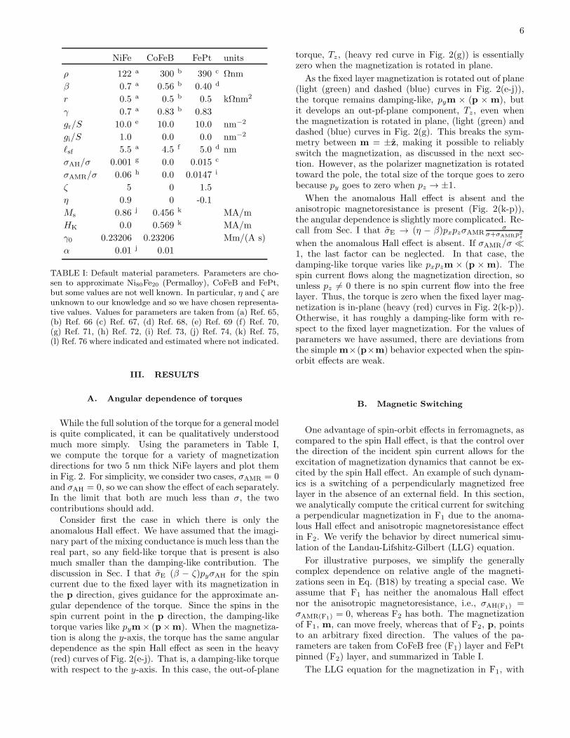
TABLE I: Default material parameters. Parameters are cho-sen to approximate Ni80Fe20 (Permalloy), CoFeB and FePt,but some values are not well known. In particular, η and ζ areunknown to our knowledge and so we have chosen representa-tive values. Values for parameters are taken from (a) Ref. 65,(b) Ref. 66 (c) Ref. 67, (d) Ref. 68, (e) Ref. 69 (f) Ref. 70,(g) Ref. 71, (h) Ref. 72, (i) Ref. 73, (j) Ref. 74, (k) Ref. 75,(l) Ref. 76 where indicated and estimated where not indicated.

III. RESULTS

A. Angular dependence of torques

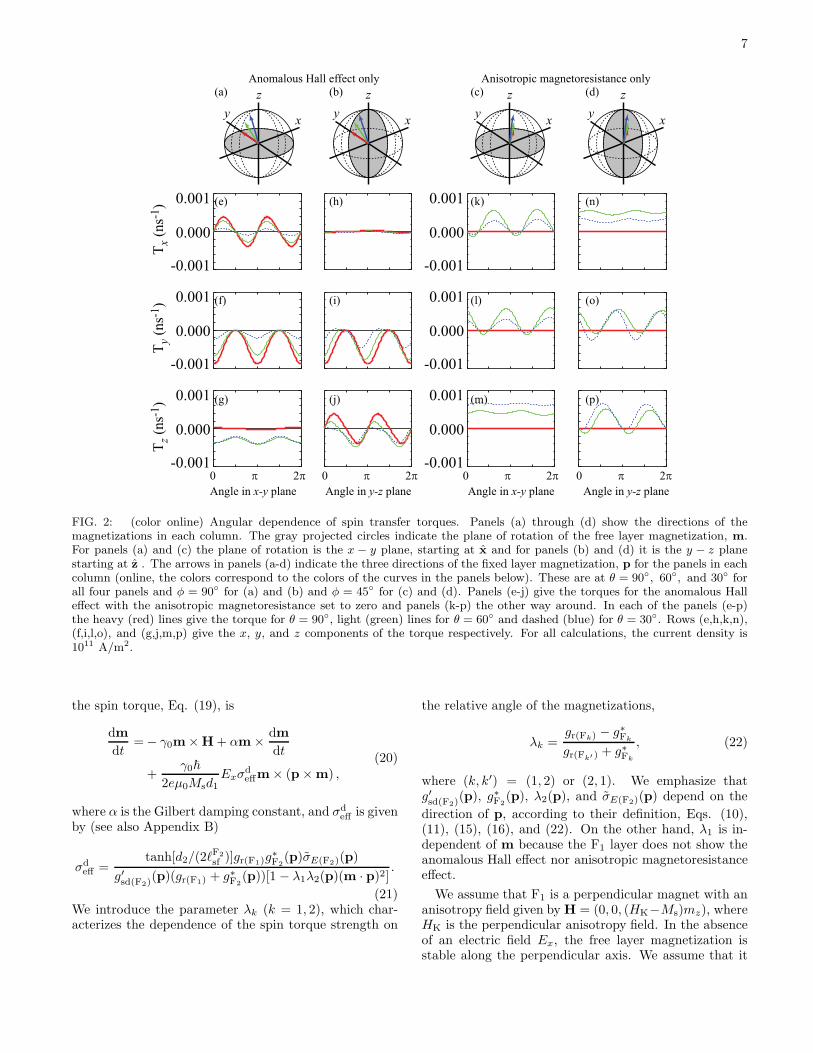
While the full solution of the torque for a general modelis quite complicated, it can be qualitatively understoodmuch more simply. Using the parameters in Table I,we compute the torque for a variety of magnetizationdirections for two 5 nm thick NiFe layers and plot themin Fig. 2. For simplicity, we consider two cases, σAMR = 0and σAH = 0, so we can show the effect of each separately.In the limit that both are much less than σ, the twocontributions should add.Consider first the case in which there is only the

anomalous Hall effect. We have assumed that the imagi-nary part of the mixing conductance is much less than thereal part, so any field-like torque that is present is alsomuch smaller than the damping-like contribution. Thediscussion in Sec. I that σE (β − ζ)pyσAH for the spincurrent due to the fixed layer with its magnetization inthe p direction, gives guidance for the approximate an-gular dependence of the torque. Since the spins in thespin current point in the p direction, the damping-liketorque varies like pym× (p×m). When the magnetiza-tion is along the y-axis, the torque has the same angulardependence as the spin Hall effect as seen in the heavy(red) curves of Fig. 2(e-j). That is, a damping-like torquewith respect to the y-axis. In this case, the out-of-plane

torque, Tz, (heavy red curve in Fig. 2(g)) is essentiallyzero when the magnetization is rotated in plane.

As the fixed layer magnetization is rotated out of plane(light (green) and dashed (blue) curves in Fig. 2(e-j)),the torque remains damping-like, pym × (p × m), butit develops an out-pf-plane component, Tz, even whenthe magnetization is rotated in plane, (light (green) anddashed (blue) curves in Fig. 2(g). This breaks the sym-metry between m = ±z, making it possible to reliablyswitch the magnetization, as discussed in the next sec-tion. However, as the polarizer magnetization is rotatedtoward the pole, the total size of the torque goes to zerobecause py goes to zero when pz → ±1.

When the anomalous Hall effect is absent and theanisotropic magnetoresistance is present (Fig. 2(k-p)),the angular dependence is slightly more complicated. Re-call from Sec. I that σE → (η − β)pxpzσAMR

σσ+σAMRp2

z

when the anomalous Hall effect is absent. If σAMR/σ ≪1, the last factor can be neglected. In that case, thedamping-like torque varies like pxpzm × (p × m). Thespin current flows along the magnetization direction, sounless pz 6= 0 there is no spin current flow into the freelayer. Thus, the torque is zero when the fixed layer mag-netization is in-plane (heavy (red) curves in Fig. 2(k-p)).Otherwise, it has roughly a damping-like form with re-spect to the fixed layer magnetization. For the values ofparameters we have assumed, there are deviations fromthe simple m×(p×m) behavior expected when the spin-orbit effects are weak.

B. Magnetic Switching

One advantage of spin-orbit effects in ferromagnets, ascompared to the spin Hall effect, is that the control overthe direction of the incident spin current allows for theexcitation of magnetization dynamics that cannot be ex-cited by the spin Hall effect. An example of such dynam-ics is a switching of a perpendicularly magnetized freelayer in the absence of an external field. In this section,we analytically compute the critical current for switchinga perpendicular magnetization in F1 due to the anoma-lous Hall effect and anisotropic magnetoresistance effectin F2. We verify the behavior by direct numerical simu-lation of the Landau-Lifshitz-Gilbert (LLG) equation.

For illustrative purposes, we simplify the generallycomplex dependence on relative angle of the magneti-zations seen in Eq. (B18) by treating a special case. Weassume that F1 has neither the anomalous Hall effectnor the anisotropic magnetoresistance, i.e., σAH(F1) =σAMR(F1) = 0, whereas F2 has both. The magnetizationof F1, m, can move freely, whereas that of F2, p, pointsto an arbitrary fixed direction. The values of the pa-rameters are taken from CoFeB free (F1) layer and FePtpinned (F2) layer, and summarized in Table I.

The LLG equation for the magnetization in F1, with

7

-0.001

0.000

0.001

-0.001

0.000

0.001

-0.001

0.000

0.001

-0.001

0.000

0.001

-0.001

0.000

0.001

-0.001

0.000

0.001

yx

z

yx

z

yx

z

yx

z

Anisotropic magnetoresistance onlyAnomalous Hall effect only

0 π 2π 0 π 2π 0 π 2π 0 π 2π

Angle in x-y plane Angle in y-z plane Angle in x-y plane Angle in y-z plane

Tx (

ns-

1)

Ty (

ns-

1)

Tz

(ns-

1)

(a)

(e)

(f)

(g)

(b)

(h)

(i)

(j)

(c)

(k)

(l)

(m)

(d)

(n)

(o)

(p)

FIG. 2: (color online) Angular dependence of spin transfer torques. Panels (a) through (d) show the directions of themagnetizations in each column. The gray projected circles indicate the plane of rotation of the free layer magnetization, m.For panels (a) and (c) the plane of rotation is the x − y plane, starting at x and for panels (b) and (d) it is the y − z planestarting at z . The arrows in panels (a-d) indicate the three directions of the fixed layer magnetization, p for the panels in eachcolumn (online, the colors correspond to the colors of the curves in the panels below). These are at θ = 90, 60, and 30 forall four panels and φ = 90 for (a) and (b) and φ = 45 for (c) and (d). Panels (e-j) give the torques for the anomalous Halleffect with the anisotropic magnetoresistance set to zero and panels (k-p) the other way around. In each of the panels (e-p)the heavy (red) lines give the torque for θ = 90, light (green) lines for θ = 60 and dashed (blue) for θ = 30. Rows (e,h,k,n),(f,i,l,o), and (g,j,m,p) give the x, y, and z components of the torque respectively. For all calculations, the current density is1011 A/m2.

the spin torque, Eq. (19), is

dm

dt=− γ0m×H+ αm × dm

dt

+γ0~

2eµ0Msd1Exσ

deffm× (p×m) ,

(20)

where α is the Gilbert damping constant, and σdeff is given

by (see also Appendix B)

σdeff =

tanh[d2/(2ℓF2

sf )]gr(F1)g∗F2(p)σE(F2)(p)

g′sd(F2)(p)(gr(F1) + g∗F2

(p))[1 − λ1λ2(p)(m · p)2] .

(21)We introduce the parameter λk (k = 1, 2), which char-acterizes the dependence of the spin torque strength on

the relative angle of the magnetizations,

λk =gr(Fk) − g∗Fk

gr(Fk′) + g∗Fk

, (22)

where (k, k′) = (1, 2) or (2, 1). We emphasize thatg′sd(F2)

(p), g∗F2(p), λ2(p), and σE(F2)(p) depend on the

direction of p, according to their definition, Eqs. (10),(11), (15), (16), and (22). On the other hand, λ1 is in-dependent of m because the F1 layer does not show theanomalous Hall effect nor anisotropic magnetoresistanceeffect.

We assume that F1 is a perpendicular magnet with ananisotropy field given by H = (0, 0, (HK−Ms)mz), whereHK is the perpendicular anisotropy field. In the absenceof an electric field Ex, the free layer magnetization isstable along the perpendicular axis. We assume that it

8

starts along the z-axis, i.e., m = z. In the presence of thespin torque, the magnetization is destabilized, and startsto precess around the z-axis. Assuming that mz ≃ 1 and|mx|, |my| ≪ 1, we can linearize the LLG equation (seeAppendix C) and determine the critical current

jcrit =− 2αeµ0Msd1(HK −Ms)

~ tanh[d2/(2ℓF2

sf )]

×(1 − λ1λ2p

2z)

2g′sd(F2)(gr(F1) + g∗F2

)σF2

(1− λ1λ2)pzg∗F2gr(F1)σE(F2)

.

(23)

Using Eq. (23), we can estimate the critical currentfor field-free switching of perpendicular layers. As anexample, let us assume that F2 has the anomalous Halleffect only, i.e., σAH(F2) 6= 0 and σAMR(F2) = 0. In thiscase, σE(F2) is (βF2

− ζF2)pyσAH(F2) and Eq. (23) can

be simplified to Eq. (C3). We choose the pinned layer

magnetization to be p = (0, 1/√2, 1/

√2) and take the

parameter values given in Table I. For 10 nm of FePt,which can be fixed in a partially out of plane configura-tion, as a polarizer and 1 nm of CoFeB, with perpendic-ular anisotropy, as a free layer, we find a critical currentof 1.0× 1012 A/m2 from Eq. (23). In Fig. 3, we show themagnetization dynamics obtained by numerically solvingthe LLG equation (20) for the electric current densitiesof (a) j = 0.9 × jc and (b) j = 1.5 × jc, respectively.The magnetization stays near the initial direction in (a),whereas it switches the direction to m = −z, showingthe validity of Eq. (23).

Figure 4 shows the switching current as a functionof the orientation of the fixed layer magnetization p =(sin(θfixed) cos(φfixed), sin(θfixed) sin(φfixed), cos(θfixed))from Eq. (23), and verified by numerical simulation ofthe LLG equation. The three panels show switching dueto the anomalous Hall effect and anisotropic magnetore-sistance separately and combined. For the parameterschosen here, given in Table I, the anomalous Hall effectis more efficient. The figure shows that the most efficientswitching occurs when the polarizer magnetization isclose to perpendicular (θfixed ≈ 0). The efficiency isdetermined by a competition between two effects. Oneeffect is the efficiency of the spins at destabilizing themagnetization toward reversal. Spins injected perpen-dicular to the stable magnetization direction exert thegreatest torque, but since they enhance precession onlyover half a period and suppress it over the other, theydo not destabilize the magnetization. Electrons withmoments antiparallel to the magnetization exert notorque, but when the magnetization fluctuates, theyexert a torque that destabilizes the magnetization overthe whole precession period. When the critical currentis large enough, they overcome the damping and anyfluctuations get magnified, leading to reversal. Thecounterbalancing effect is that when the pinned layermagnetization is collinear with the magnetization, it isalso collinear with the film normal and the injected spincurrent goes to zero. So, the most efficient switching

mag

netiz

atio

n

(b)

(a)

0

-0.5

0.5

1.0

-1.0

mx

my

mz

j=0.9×jc, p=(ey+ez)/√2

time (ns)

mag

netiz

atio

n

(c)

0

-0.5

0.5

1.0

-1.00 10 20 30 40 50

mx

my

mz

j=1.5×jc, p=(ey+ez)/√2

my

x

z

p

θfixed

φfixed

FIG. 3: (color online) Magnetization dynamics due to theanomalous Hall effect. Panel (a) shows the geometry. Thetrajectories obtained by numerically solving the LLG equation(20) are shown in (b) for j = 0.9× jc and (c) for j = 1.5× jc.

occurs with the pinned layer magnetization close tonormal but not all the way there, maximizing thetotal perpendicular component of the injected spins.Switching due to the anomalous Hall effect and that dueto anisotropic magnetoresistance depend differently onthe azimuthal angle so for some orientations of the fixedlayer magnetization, they compete, but for others theycooperate to reduce the critical current.

The critical current is minimized at an optimal direc-tion of p. Because of complex dependences of σE and σδµ

on the magnetization direction, as shown in Eqs. (10)and (11), it is difficult to derive a formula of this optimaldirection. However, for the F2 with the anomalous Halleffect only, we can derive the analytical formula of theoptimum direction of p; see Appendix C1. The result,for this set of parameters is θfixed = 31.6, φfixed = 90.

We can compare these results with the magnetizationswitching assisted by the spin Hall effect. In the spin

9

0 90 180 270 360

0

45

90

135

180

0

45

90

135

180

0

45

90

135

180

Fixed layer azimuthal angle φfixed

Fix

ed l

ayer

po

lar

ang

le θ

fix

ed

(c) Both AHE and AMR

(a) AHE only

(b) AMR only

-2.0 2.0±∞

Critical current (1012 A/m2)

-1.0 1.0

4.0-4.0 0.8-0.8 1.3_

-1.3_

0.6_

-0.6_

FIG. 4: (color online) Critical currents for a CoFeB free layerand FePt fixed layer as a function of the fixed layer magne-tization direction. The contours are chosen uniformly in theinverse critical current, the contour where the critical currentsdiverge is labeled ±∞. In panel (a), we assume that the po-larizer has anomalous Hall effect (AHE) but no anisotropicmagnetoresistance (AMR). In panel (b), we assume it has theAMR but no AHE, and in panel (c) we assume it has both.Dark (blue) regions indicate regions with low critical for onedirection of current flow and light (yellow) regions indicatelow critical currents for the other direction. At the equator(θfixed = 90), the critical currents diverge for all three cases,however, for the case with only AMR [panel (b)], the signdoes not change as θfixed is varied near that point, but for theother two cases it does.

Hall effect, spin current polarized along the y directionis injected to the free layer. This situation is similar toa special case of switching by spin-orbit effects in fer-romagnets in which the pinned layer magnetization isin the y direction. It is useful to consider a general-ized situation with the fixed layer magnetization in theyz-plane, φfixed = 90 with no anisotropic magnetore-sistance. Then, σE simplifies and Eq. (23) has the fac-tor pypz in the denominator as seen in Eq. (C3). Thisfactor implies that jAH

c diverges when p points to thez-direction (py = 0 and pz = 1) because the anoma-lous Hall effect does not induce spin current along the z-direction when py = 0. The critical current also divergeswhen p points to the y-direction (py = 1 and pz = 0) be-cause the spin-transfer torque never overcomes the damp-ing torque as needed to enhance precession. This is theequivalent of switching by the spin Hall effect. While thespin-transfer torque can excite magnetization dynamics,when the fixed layer magnetization is along y it does notovercome the damping and does not cause precession tobecome unstable.It is possible to excite dynamics in perpendicularly

magnetized samples with the spin Hall effect (or theanomalous Hall effect with p = y) as shown by Lee et

al.23. In fact, they demonstrate that it is possible to

switch the magnetization. However, the switching theyobserve is not due to the spin transfer torque overcom-ing the damping, but rather is due to a large ampli-tude excitation due to the rapid onset of the currentand hence torque. However, since nothing in the sys-tem breaks the symmetry between up and down, suchswitching is extremely sensitive to pulse duration andcurrent amplitude. Lee et al.

23 demonstrate such sensi-tivity in Fig. 1(b) of their paper. They derive an ana-lytic form, Eq. (5), for the critical current that is inde-pendent of the damping parameter. This independenceindicates that the switching mechanism is precessional,rather than due to overcoming damping. To switch themagnetization direction without such sensitivity, an in-plane magnetic field slightly tilted to the z-direction hasbeen used experimentally77. The switching mechanismdue to the anomalous Hall effect with a fixed layer withan out-of-plane component to the magnetization has theadvantage of being largely independent of the currentdensity or pulse duration for currents above the criticalcurrent. Another advantage is that the external field isunnecessary to switch the magnetization. It can also besignificantly lower when the damping parameter is small,as is desirable in many magnetic devices.

C. Domain wall motion

The spin-orbit torques generated by ferromagnets canalso be useful to displace in-plane magnetic domain walls,which we illustrate through two simple examples. Wefirst consider the spin-valve illustrated in Fig. 5(a), withan in-plane domain wall in the free layer F1 and a uni-

10

Do

mai

n w

all

vel

oci

ty (

m/s

)

Out-of-plane polarizer angle, θ (°)

0 15 30 45 60 75 90

0

300

0

0.0

1.0

(a)

(b)

(c)

φ (°)

z

m

y xp θ

φ

FIG. 5: (color online) (a) Schematic of the spin valve witha transverse in-plane wall and a fixed uniform polarizer. (b)Out-of-plane tilt angle of domain wall and (c) Domain wallvelocity as a function of the out-of-plane angle θ of the po-larizer. Calculations are done for 10 nm Py for a polarizerlayer, 1 nm Py for a free layer, and a charge current densityof 2× 1011 A/m2.

form polarizer p = (0, py, pz) in the fixed layer F2. Dueto the spin orbit effects in F2, a torque is generated on F1that has the form : T = τso(m,p) m×(m×p). To studythe effect of this torque we consider a 1D model78 of atransverse wall profile with a domain wall width ∆. Themagnetization in the free layer, with the domain wall, issubject to a spin current from a fixed layer below. Thisspin current will cause a small tilting of the magnetiza-tion away from the long axis in all of the domains and willcause motion of the domain wall. We neglect the smalltilting of the domains to get the following equations forthe domain wall dynamics:

φ+α

∆q = τsopz cosφ− τsopy sinφ (24)

q

∆− αφ = γ0Hk sinφ cosφ (25)

Here q is the domain wall position, φ the out-of-planetilt angle and Hk the shape anisotropy. At equilibriumin the absence of spin torques, φ is equal to zero and thedomain wall lies in plane.

In the regime below Walker breakdown, the wall moveswith a constant tilt angle and a steady velocity. Assum-ing the tilt is small, sinφ ≪ 1,

φ =τsopz

αγ0Hk + τsopy

qAH =∆

ατsopz

αγ0Hk

αγ0Hk + τsopy(26)

Since αγ0Hk ≫ τso for typical values of the current den-sity, the out-of-plane tilt is indeed small. The domainwall moves steadily only if the generated spin torquehas a component along the z-direction. This is not thecase of the torque generated by pure spin Hall effect ina non-magnetic heavy metal, in which case the domainwall does not move.79 On the other hand, the spin-orbittorques generated by a ferromagnet can have componentsalong both the z and y directions when the polarizeris tilted out-of-plane. If, as we did in the last section,we consider the case of the torque generated by just theanomalous Hall effect in F2, then

τAH =γ0~

2eµ0Ms

tanh[d2/(2ℓsf)]

d1

g∗grg′sd(gr + g∗)

1

1− λ2(m · p)2 (β − ζ)σAHExpy (27)

This behavior is shown in Fig. 5, in which we treat themotion for the case with the anomalous Hall effect andanisotropic magnetoresistance in both layers. However,since we assume the magnetization lies in the y−z plane,the anisotropic magnetoresistance plays a negligible role.Fig. 5 shows a relatively large domain wall velocity for amodest charge current density of 2 × 1011 A/m2 and avery small out of plane tilt of less than a degree.

In the proposed spin-valve system, the current flowingin the ferromagnet F1 through the domain wall will alsogive rise to the more familiar (intralayer) adiabatic andnon-adiabatic spin-transfer torques on the domain wall,these can enhance or oppose the effect of the spin-orbittorques. In comparison, the domain wall velocity inducedby these intralayer torques is :

qna =1

α

γ0~

2eµ0MsPβnaσEx (28)

where P ≈ β is the current polarization and βna the pro-portionality factor between the non-adiabatic and adia-batic torques. The ratio of the velocities is

qAH

qna≈ ∆

d1

pypz(β − ζ)σAH

PβnaσF, (29)

where F is a series of factors (see Eq. (27) of order one.In a typical material as NiFe, both the anomalous spinhall angle and the non-adiabatic parameter βna are closeto 1 %50. However, the domain wall will be mainly drivenby the anomalous Hall torque because the wall width istypically much bigger than the layer thickness ∆/d > 10

11

0 10 20 30 400

4

8

12

16

out-

of-

pla

ne

tilt

ang

le o

f th

e D

W (

°)

spacer thickness tNM

(nm)

bottom

(a)

(c)

top

(b)

z

m

yx

φ

p

φ

F1

F2

FIG. 6: (color on-line) (a) Schematic of the spin valve inanti-parallel configuration with two domain walls, one in eachlayer. (b) micromagnetic simulations of the coupled domainwall system showing in blue the positive z component of themagnetization. (c) Maximum out-of-plane tilt angle φ of themagnetization in the domain wall as a function of the spacerthickness.

for most systems.80

The other system we consider is the coupled domainwall system shown in Fig. 6(a). In the case of a fixedpolarizer F2 and a free layer F1, F2 can exert a torqueon F1. But if F2 is no longer fixed, F1 can also induce atorque on F2. If the magnetic configuration is well cho-sen, these reciprocal torques can add and enhance mag-netization dynamics of the coupled system. This is thecase for the double domain wall system with anti-parallelconfiguration shown in Fig. 6.If both magnetic layers are unpinned, the domain walls

in each layer are strongly coupled. Domain walls in wireswith opposite in-plane magnetizations tilt out of planesignificantly due to the dipolar interaction between them,as shown in Fig.6. In equilibrium, one domain wall hasthe out-of-plane tilt angle φ0, and the other π − φ0 sothat the out-of-plane component is in the same directionand the in-plane directions are opposite. This configu-ration is illustrated in the micromagnetic simulations inFig. 6(b) where blue shows the out-of-plane componentof the magnetization.81 As the spacer thickness tNM de-

creases, the dipolar fields on each domain wall increase,and the maximum out-of-plane tilt angle increases asshown in Fig. 6(b), reaching values close to 15 for spacerthicknesses typical of synthetic antiferromagnets.In this configuration, the domain wall in F2 polarizes

the domain wall in F1 (and reciprocally), and we canreplace py and pz respectively by −cosφ and sinφ inEq. (24). For small angle deviations from the equilib-rium configuration, this immediately leads to

qAH =∆

ατso sin(2φ0) (30)

Due to the particular symmetry of the anomalous Halleffect torques, the domain wall in F2 acquires the samevelocity: the motion of the coupled domain wall systemis self-sustained. For small spacer thicknesses, the tiltangle is large, and velocities comparable to the singlewall system with a uniform tilted fixed polarizer can bereached.

IV. SUMMARY

In this paper we develop a drift-diffusion approach totreat transport effects of spin-orbit coupling in ferromag-nets. These include the anomalous Hall effect and theanisotropic magnetoresistance. In addition to the trans-verse charge currents that arise due to these effects, thereare concomitant spin currents. These spin currents flowperpendicularly to the electric field, and so can be in-jected into layers perpendicular to the electrical currentflow. When these other layers are ferromagnets withmagnetizations that are not aligned with the originallayer, they create spin transfer torques. Unlike the re-lated spin Hall effect in non-magnetic materials, the fer-romagnetic spin-orbit effects allow some control of theorientation of the injected spins. This control arises be-cause the flowing spins in a ferromagnet are collinear withthe magnetization. Changing the orientation of the mag-netization changes the direction of the spins injected intoother layers.We compute the torques due to current flow for two fer-

romagnet layers separated by a thin non-magnetic layer.The control of the direction of the injected spins makesit is possible to switch perpendicularly magnetized layersmore easily because of the possibility of an out-of-planecomponent of the torque. We also show that such torquesmake it possible to switch in-plane magnetized layers viapropagation of transverse/vortex walls and can efficientlyinduce dynamics in coupled magnetic systems, e.g. cou-pled transverse domain walls.

Acknowledgments

The authors thank Robert McMichael for useful dis-cussions. JG acknowledges funding from the European

12

Research Council Grant No. 259068.

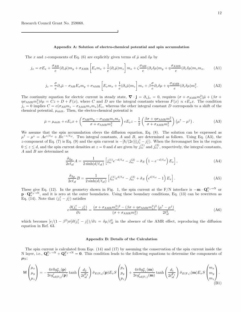
Appendix A: Solution of electro-chemical potential and spin accumulation

The x and z-components of Eq. (6) are explicitly given terms of µ and δµ by

jx = σEx +σAH

e(∂zµ)my + σAMR

[

Exmx +1

e(∂zµ)mz

]

mx + ζσAH

e(∂zδµ)my + η

σAMR

e(∂zδµ)mzmx, (A1)

jz =σ

e∂zµ− σAHExmy + σAMR

[

Exmx +1

e(∂zµ)mz

]

mz + βσ

e∂zδµ+ η

σAMR

e(∂zδµ)m

2z. (A2)

The continuity equation for electric current in steady state, ∇ · j = ∂zjz = 0, requires (σ + σAMRm2z)µ + (βσ +

ησAMRm2z)δµ = Cz + D + F (x), where C and D are the integral constants whereas F (x) ∝ eExx. The condition

jz = 0 implies C = e(σAHmz − σAMRmzmx)Ex, whereas the other integral constant D corresponds to a shift of thechemical potential, µshift. Then, the electro-chemical potential is

µ = µshift + eExx+

(

σAHmy − σAMRmzmx

σ + σAMRm2z

)

eExz −1

2

(

βσ + ησAMRm2z

σ + σAMRm2z

)

(

µ↑ − µ↓)

. (A3)

We assume that the spin accumulation obeys the diffusion equation, Eq. (8). The solution can be expressed asµ↑ − µ↓ = Aez/ℓsf + Be−z/ℓsf . Two integral constants, A and B, are determined as follows. Using Eq. (A3), thez-component of Eq. (7) is Eq. (9) and the spin current is −[~/(2e)](j↑z − j↓z ). When the ferromagnet lies in the region

0 ≤ z ≤ d, and the spin current densities at z = 0 and d are given by j(1)sz and j

(2)sz , respectively, the integral constants,

A and B are determined as

σδµ

2eℓsfA =

1

2 sinh(d/ℓsf)

[

j(1)sz e−d/ℓsf − j(2)sz − σE

(

1− e−d/ℓsf)

Ex

]

, (A4)

σδµ

2eℓsfB =

1

2 sinh(d/ℓsf)

[

j(1)sz ed/ℓsf − j(2)sz + σE

(

ed/ℓsf − 1)

Ex

]

. (A5)

These give Eq. (12). In the geometry shown in Fig. 1, the spin current at the F/N interface is −m · QF1→Ns or

p · QF2→Ns , and it is zero at the outer boundaries. Using these boundary conditions, Eq. (13) can be rewritten as

Eq. (14). Note that (j↑z − j↓z ) satisfies

e∂(j↑z − j↓z )

∂z=

(σ + σAMRm2z)

2 − (βσ + ησAMRm2z)

2

(σ + σAMRm2z)

(µ↑ − µ↓)

2ℓ2sf, (A6)

which becomes [e/(1 − β2)σ]∂(j↑z − j↓z )/∂z = δµ/ℓ2sf in the absence of the AMR effect, reproducing the diffusionequation in Ref. 63.

Appendix B: Details of the Calculation

The spin current is calculated from Eqs. (14) and (17) by assuming the conservation of the spin current inside theN layer, i.e., QF1→N

s +QF2→Ns = 0. This condition leads to the following equations to determine the components of

µN;

M

µx

µy

µz

= −

4π~g∗F2(p)

2eg′sd(F2)(p)

tanh

(

d2

2ℓF2

sf

)

σE(F2)(p)ExS

pxpypz

+

4π~g∗F1(m)

2eg′sd(F1)(m)

tanh

(

d1

2ℓF1

sf

)

σE(F1)(m)ExS

mx

my

mz

.

(B1)

13

Here, the components of the 3× 3 matrix M are given by

M1,1 = g∗F1m2

x + gr(F1)

(

1−m2x

)

+ g∗F2p2x + gr(F2)

(

1− p2x)

, (B2)

M1,2 =(

g∗F1− gr(F1)

)

mxmy + gi(F1)mz +(

g∗F2− gr(F2)

)

pxpy + gi(F2)pz, (B3)

M1,3 =(

g∗F1− gr(F1)

)

mzmx − gi(F1)my +(

g∗F2− gr(F2)

)

pzpx − gi(F2)py, (B4)

M2,1 =(

g∗F1− gr(F1)

)

mxmy − gi(F1)mz +(

g∗F2− gr(F2)

)

pxpy − gi(F2)pz, (B5)

M2,2 = g∗F1m2

y + gr(F1)

(

1−m2y

)

+ g∗F2p2y + gr(F2)

(

1− p2y)

, (B6)

M2,3 =(

g∗F1− gr(F1)

)

mymz + gi(F1)mx +(

g∗F2− gr(F2)

)

pypz + gi(F2)px, (B7)

M3,1 =(

g∗F1− gr(F1)

)

mzmx + gi(F1)my +(

g∗F2− gr(F2)

)

pzpx + gi(F2)py, (B8)

M3,2 =(

g∗F1− gr(F1)

)

mymz − gi(F1)mx +(

g∗F2− gr(F2)

)

pypz − gi(F2)px, (B9)

M3,3 = g∗F1m2

z + gr(F1)

(

1−m2z

)

+ g∗F2p2z + gr(F2)

(

1− p2z)

. (B10)

The solution of µN = (µx, µy, µz) can be obtained by calculating the inverse of M. In Eq. (B1), we added ”(p)”and ”(m)” after g∗, g′sd, and σE to emphasize that these quantities depend explicitly on the magnetization directionthrough Eqs. (10), (11), (15), and (16). From µ we evaluate the spin currents, Eqs. (14) and (17). The LLG equationsfor m and p are, respectively, given by

dm

dt= −γ0m×H+

γ0µ0MsV

m×(

QF1→Ns ×m

)

+ αm × dm

dt, (B11)

dp

dt= −γ0p×H+

γ0µ0MsV

p×(

QF2→Ns × p

)

+ αp× dp

dt, (B12)

where γ0 and α are the gyromagnetic ratio and Gilbert damping constant, respectively. The volume is V .

1. Special cases for the spin torque

Although it is possible to solve Eq. (B1) analytically for an arbitrary magnetization alignment, the solution lookscomplicated. However, relatively simple analytical formulas can be obtained in some special cases. In this section,we discuss such cases. Note that Eq. (B1) comes from the conservation law for spin current inside the normal metallayer, QF1→N

s +QF2→Ns = 0, which can be written as

g∗F1(m · µN)m+ gr(F1)m× (µN ×m) + gi(F1)µN ×m

+ g∗F2(p · µN)p+ gr(F2)p× (µN × p) + gi(F2)µN × p

= s1m− s2p,

(B13)

where sk = [4π~g∗Fk/(2eg′sd(Fk)

)] tanh[dk/(2ℓFk

sf )]σE(Fk)ExS (k = 1, 2): see Eq. (B1). We expand µN as

µN = amm+ bmm× p+ cmm× (p×m) . (B14)

Substituting this expression into Eq. (B13), and using the simplification gi = 0, the coefficients am, bm, and cm are

am =[(gr(F1) + g∗F2

) + (gr(F2) − g∗F2)(m · p)2]s1 − (gr(F1) + gr(F2))m · ps2

(gr(F1) + g∗F2)(gr(F2) + g∗F1

)− (gr(F1) − g∗F1)(gr(F2) − g∗F2

)(m · p)2 , (B15)

bm = 0, (B16)

cm =(gr(F2) − g∗F2

)m · ps1 − (gr(F2) + g∗F1)s2

(gr(F1) + g∗F2)(gr(F2) + g∗F1

)− (gr(F1) − g∗F1)(gr(F2) − g∗F2

)(m · p)2 . (B17)

The spin torque acting on the magnetization of the F1 layer, m, is [γ0/(µ0MsV )]m × (QF1→Ns × m) =

−[γ0gr/(4πµ0MsV )]m× (µN×m). Then, the coefficient cm and its direction m× (p×m) gives the spin torque. The

14

explicit form of the spin torque acting on m is

dm

dt=

γ0~Ex

2eµ0M1d1gr(F1)

m× (p×m)

1− λ1(m)λ2(p)(m · p)2 ,

×

g∗F2(p) tanh[d2/(2ℓ

F2

sf )]σE(F2)(p)

g′sd(F2)(p)[gr(F1) + g∗F2

(p)]− λ2(p)

g∗F1(m) tanh[d2/(2ℓ

F1

sf )]σE(F1)(m)

g′sd(F1)(m)[gr(F1) + g∗F2

(p)]m · p

(B18)

where λk is defined by Eq. (22). Note that the conductance g∗ and g′sd, and therefore λ, depend on not only thematerial parameters but also the magnetization direction when the anisotropic magnetoresistance effect is finite; seeEqs. (11), (15), and (16). Also, σE depends on the magnetization direction, as shown in Eq. (10). Therefore, weadd ”(m)” or ”(p)” after g∗Fk

, gsd(Fk), σE(Fk), and λk to emphasize the fact that these depend on the magnetizationdirection, m or p. Similarly, the spin torque acting on the magnetization of the F2 layer is given by

dp

dt=− γ0~Ex

2eµ0M2d2gr(F2)

p× (m× p)

1− λ1(m)λ2(p)(m · p)2 ,

×

g∗F1(m) tanh[d1/(2ℓ

F1

sf )]σE(F1)(m)

g′sd(F1)(m)[gr(F2) + g∗F1

(m)]− λ1(m)

g∗F2(p) tanh[d2/(2ℓ

F2

sf )]σE(F2)(p)

g′sd(F2)(p)[gr(F2) + g∗F1

(m)]m · p

(B19)

These formulas can be simplified in the absence of the anisotropic magnetoresistance effect, which we show in thefollowing sections.

a. When σAMR = 0 and only the F2 has an anomalous Hall effect

In the absence of the anisotropic magnetoresistance effect, i.e., σAMR = 0, g∗, g′sd, and λ become independent fromthe magnetization directions. In this section, we also assume that the material parameters are identical between twoferromagnets, for simplicity. In this case, many of the derived parameters become independent of the layer and wesuppress those indices.

Since σE of the F1 layer is zero and that of the F2 layer is σE(F2) = (β − ζ)σAHpy. The conductance gsd, Eq. (16),

and g∗, Eq. (15), are independent of the magnetization direction because σδµ = (1 − β2)σ is independent of themagnetization direction. Then, from Eq. (B18), the spin torque acting on m is

dm

dt=

γ0~

2eMsd

g∗gr(β − ζ) tanh[d/(2ℓsf)]σAHEx

g′sd(gr + g∗)py

m× (p×m)

1− λ2(m · p)2 . (B20)

Similarly, the spin torque acting on the F2 layer, p, is obtained from Eq. (B19) as

dp

dt=

γ0~

2eµ0Msd

g∗gr(β − ζ) tanh[d/(2ℓsf)]σAHEx

g′sd(gr + g∗)pyλm · p p× (m × p)

1− λ2(m · p)2 . (B21)

b. When σAMR = 0 and both the F1 and F2 layers show the anomalous Hall effect

In this case, σE of the F1 and F2 layers are given by (β − ζ)σmy and (β − ζ)σpy , respectively. The spin torquesacting on m and p are obtained from Eqs. (B18) and (B19) as

dm

dt=

γ0~

2eµ0Msd

g∗gr(β − ζ) tanh[d/(2ℓsf)]σAHEx

g′sd(gr + g∗)

[

py −myλm · p1− λ2(m · p)2

]

m× (p×m) . (B22)

dp

dt=

γ0~

2eµ0Msd

g∗gr(β − ζ) tanh[d/(2ℓsf)]σAHEx

g′sd(gr + g∗)

[

pyλm · p−my

1− λ2(m · p)2]

p× (m× p) . (B23)

15

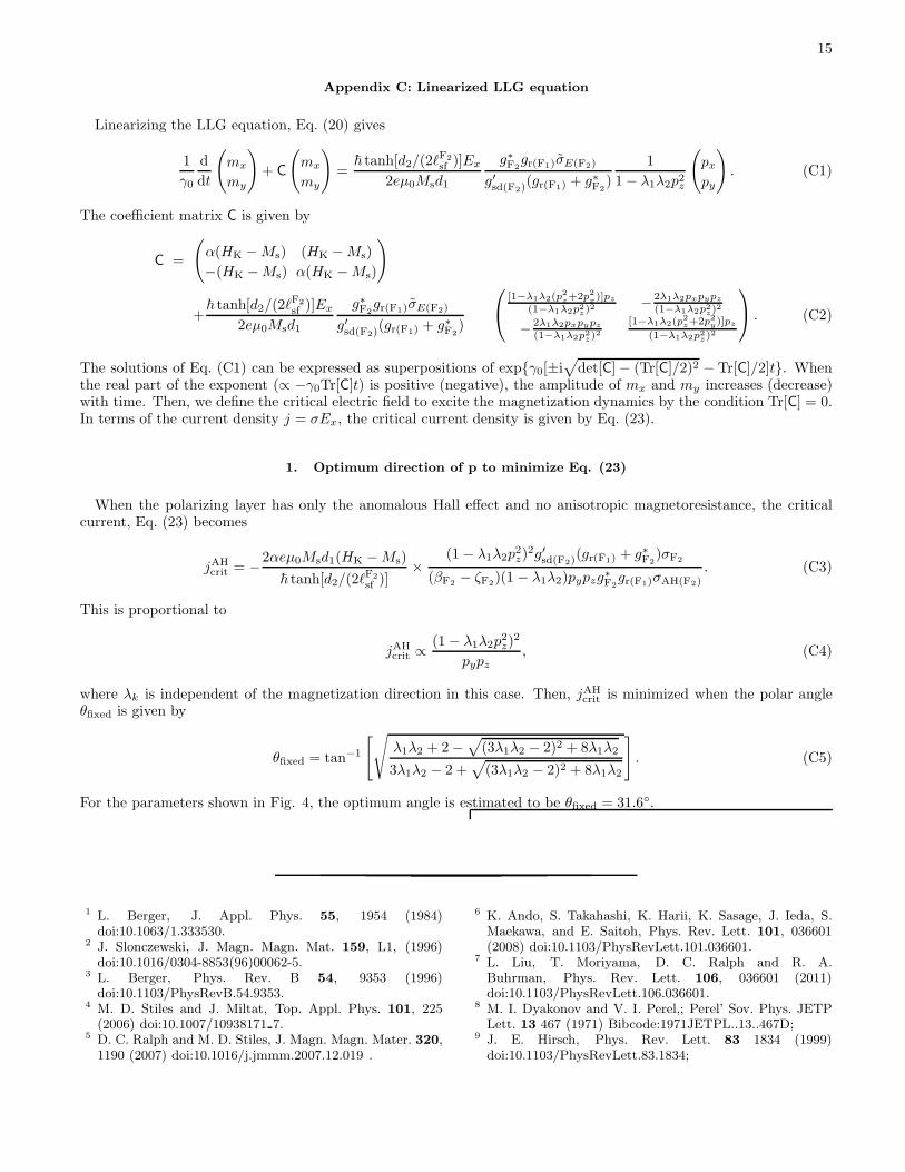
Appendix C: Linearized LLG equation

Linearizing the LLG equation, Eq. (20) gives

1

γ0

d

dt

(

mx

my

)

+ C

(

mx

my

)

=~ tanh[d2/(2ℓ

F2

sf )]Ex

2eµ0Msd1

g∗F2gr(F1)σE(F2)

g′sd(F2)(gr(F1) + g∗F2

)

1

1− λ1λ2p2z

(

pxpy

)

. (C1)

The coefficient matrix C is given by

C =

(

α(HK −Ms) (HK −Ms)

−(HK −Ms) α(HK −Ms)

)

+~ tanh[d2/(2ℓ

F2

sf )]Ex

2eµ0Msd1

g∗F2gr(F1)σE(F2)

g′sd(F2)(gr(F1) + g∗F2

)

[1−λ1λ2(p2

z+2p2

x)]pz

(1−λ1λ2p2z)

2 − 2λ1λ2pxpypz

(1−λ1λ2p2z)

2

− 2λ1λ2pxpypz

(1−λ1λ2p2z)

2

[1−λ1λ2(p2

z+2p2

y)]pz

(1−λ1λ2p2z)

2

. (C2)

The solutions of Eq. (C1) can be expressed as superpositions of expγ0[±i√

det[C]− (Tr[C]/2)2 − Tr[C]/2]t. Whenthe real part of the exponent (∝ −γ0Tr[C]t) is positive (negative), the amplitude of mx and my increases (decrease)with time. Then, we define the critical electric field to excite the magnetization dynamics by the condition Tr[C] = 0.In terms of the current density j = σEx, the critical current density is given by Eq. (23).

1. Optimum direction of p to minimize Eq. (23)

When the polarizing layer has only the anomalous Hall effect and no anisotropic magnetoresistance, the criticalcurrent, Eq. (23) becomes

jAHcrit = −2αeµ0Msd1(HK −Ms)

~ tanh[d2/(2ℓF2

sf )]×

(1− λ1λ2p2z)

2g′sd(F2)(gr(F1) + g∗F2

)σF2

(βF2− ζF2

)(1 − λ1λ2)pypzg∗F2gr(F1)σAH(F2)

. (C3)

This is proportional to

jAHcrit ∝

(1 − λ1λ2p2z)

2

pypz, (C4)

where λk is independent of the magnetization direction in this case. Then, jAHcrit is minimized when the polar angle

θfixed is given by

θfixed = tan−1

[√

λ1λ2 + 2−√

(3λ1λ2 − 2)2 + 8λ1λ2

3λ1λ2 − 2 +√

(3λ1λ2 − 2)2 + 8λ1λ2

]

. (C5)

For the parameters shown in Fig. 4, the optimum angle is estimated to be θfixed = 31.6.

1 L. Berger, J. Appl. Phys. 55, 1954 (1984)doi:10.1063/1.333530.

2 J. Slonczewski, J. Magn. Magn. Mat. 159, L1, (1996)doi:10.1016/0304-8853(96)00062-5.

3 L. Berger, Phys. Rev. B 54, 9353 (1996)doi:10.1103/PhysRevB.54.9353.

4 M. D. Stiles and J. Miltat, Top. Appl. Phys. 101, 225(2006) doi:10.1007/10938171 7.

5 D. C. Ralph and M. D. Stiles, J. Magn. Magn. Mater. 320,1190 (2007) doi:10.1016/j.jmmm.2007.12.019 .

6 K. Ando, S. Takahashi, K. Harii, K. Sasage, J. Ieda, S.Maekawa, and E. Saitoh, Phys. Rev. Lett. 101, 036601(2008) doi:10.1103/PhysRevLett.101.036601.

7 L. Liu, T. Moriyama, D. C. Ralph and R. A.Buhrman, Phys. Rev. Lett. 106, 036601 (2011)doi:10.1103/PhysRevLett.106.036601.

8 M. I. Dyakonov and V. I. Perel,; Perel’ Sov. Phys. JETPLett. 13 467 (1971) Bibcode:1971JETPL..13..467D;

9 J. E. Hirsch, Phys. Rev. Lett. 83 1834 (1999)doi:10.1103/PhysRevLett.83.1834;

16

10 S. Zhang, Phys. Rev. Lett. 85, 393 (2000)doi:10.1103/PhysRevLett.85.393.

11 Yu. A. Bychkov and E. I. Rashba, JETP. Lett. 39, 78(1984).

12 V. M. Edelstein, Solid State Commun. 73, 233 (1990)doi:10.1016/0038-1098(90)90963-C.

13 K. Obata, and G. Tatara, Phys Rev. B 77, 214429 (2008)doi:10.1103/PhysRevB.77.214429.

14 A. Manchon and S. Zhang, Phys. Rev. B 78, 212405 (2008)doi:10.1103/PhysRevB.78.212405.

15 A. Matos-Abiague and R. L. Rodriguez-Suarez, Phys. Rev.B 80, 094424 (2009) doi:10.1103/PhysRevB.80.094424.

16 X. Wang and A. Manchon, Phys. Rev. Lett. 108, 117201(2012) doi:10.1103/PhysRevLett.108.117201.

17 K.-W. Kim, S.-M. Seo, J. Ryu, K.-J. Lee, andH.-W. Lee, Phys. Rev. B 85, 180404(R) (2012)doi:10.1103/PhysRevB.85.180404.

18 D. A. Pesin and A. H. MacDonald, Phys. Rev. B 86,014416 (2012) doi:10.1103/PhysRevB.86.094406.

19 E. van der Bijl and R. A. Duine, Phys. Rev. B 86, 094406(2012) doi:10.1103/PhysRevB.86.094406.

20 I. M. Miron, K. Garello, G. Gaudin, P.-J. Zermatten, M.V. Costache, S. Auffret, S. Bandiera, B. Rodmacq, A.Schuhl, and P. Gambadella, Nature (London) 476, 189(2011) doi:10.1038/nmat3020.

21 L. Liu, C.-F. Pai, Y. Li, H. W. Tseng, D. C.Ralph and R. A. Buhrman, Science 4, 555 (2012)doi:10.1126/science.1218197.

22 K. Garello, C. O. Avci, I. M. Miron, O. Boulle, S. Auffret,P. Gambadella, and G. Gaudin, arXiv:1310.5586.

23 K.-S. Lee, S.-W. Lee, B.-C. Min, and K.-J. Lee, Appl.Phys. Lett. 102, 112410 (2013) doi:10.1063/1.4798288.

24 K.-S. Lee, S.-W. Lee, B.-C. Min, and K.-J. Lee, Appl.Phys. Lett. 104, 072413 (2014) doi:10.1063/1.4866186.

25 I. M. Miron, T. Moore, H. Szambolics, L. D. Buda-Prejbeanu, S. Auffret, B. Rodmacq, S. Pizzini, J. Vogel,M. Bonfim, A. Schuhl, and G. Gaudin, Nat. Mater. 10,419 (2011) doi:10.1038/nmat3020.

26 P. P. J. Haazen, E. Mure, J. H. Franken, R. Lavrijsen, H.J. M. Swagten, and B. Koopmans, Nat. Mater. 12, 299(2013) doi:10.1038/nmat3553.

27 S. Emori, U. Bauer, S.-M. Ahn, E. Martinez, and G. S. D.Beach, Nat. Mater. 12, 611 (2013) doi:10.1038/nmat3675.

28 K.-S. Ryu, L. Thomas, S.-H. Yang, and S. S. P. Parkin,Nat. Nanotech. 8, 527 (2013) doi:10.1038/nnano.2013.102.

29 Y. Yoshimura, T. Koyama, D. Chiba, Y. Nakatani,S. Fukami, M. Yamanouchi, H. Ohno, K.-J. Kim, T.Moriyama, and T. Ono, Appl. Phys. Express 7, 033005(2014).

30 S.-M. Seo, K.-W. Kim, J. Ryu, H.-W. Lee, andK.-J. Lee, Appl. Phys. Lett. 101, 022405 (2012)doi:10.1063/1.4733674.

31 A. Thiaville, S. Rohart, E. Jue, V. Cros, and A. Fert,Europhys. Lett. 100, 57002 (2012) doi:10.1209/0295-5075/100/57002.

32 J. Kim, J. Sinha, M. Hayashi, M. Yamanouchi, S. Fukami,T. Suzuki, S. Mitani, and H. Ohno, Nat. Mater. 12, 240(2013) doi:10.1038/nmat3522.

33 X. Qiu, K. Narayanapillai, Y. Wu, P. Deorani, X.Yin, A. Rusydi, K.-J. Lee, H.-W. Lee, and H. Yang,arXiv:1311.3032.

34 X. Fan, H. Celik, J. Wu, C. Ni, K.-J. Lee, V. O.Lorenz, and J. Q. Xiao, Nat. Commun. 5 3042 (2014)

doi:10.1038/ncomms4042.35 R. H. Liu, W. L. Lim, and S. Urazhdin, Phys. Rev. B 89,

220409(R) (2014) doi:10.1103/PhysRevB.89.220409.36 K. Garello, I. M. Miron, C. O. Avci, F. Freimuth,

Y. Mokrousov, S. Blugel, S. Auffret, O. Boulle, G.Gaudin, and P. Gambardella, Nat. Nanotech. 8, 587 (2013)doi:10.1038/nnano.2013.145.

37 X. Qiu, P. Deorani, K. Narayanapillai, K.-S. Lee, K.-J.Lee, H.-W. Lee, and H. Yang, Sci. Rep. 4, 4491 (2014)doi:10.1038/srep04491.

38 P. M. Haney, H.-W. Lee, K.-J. Lee, A. Manchon,and M. D. Stiles, Phys. Rev. B 87, 174411 (2013)doi:10.1103/PhysRevB.87.174411 .

39 P. M. Haney, H.-W. Lee, K.-J. Lee, A. Manchon,and M. D. Stiles, Phys. Rev. B 88, 214417 (2013)doi:10.1103/PhysRevB.88.214417 .

40 F. Freimuth, S. Blugel, Y. Mokrousov, arXiv:1305.4873.41 F. Freimuth, S. Blugel, Y. Mokrousov, J. Phys.

Condens. Matter 26, 104202 (2014) doi:10.1088/0953-8984/26/10/104202.

42 H. Kurebayashi, J. Sinova, D. Fang, A. C. Irvine, T. D.Skinner, J. Wunderlich, V. Novak, R. P. Campion, B. L.Gallagher, E. K. Vehstedt, L. P. Zarobo, K. Vyborny, A. J.Ferguson, and T. Jungwirth, Nat. Nanotech. 9, 211 (2014)doi:10.1038/nnano.2014.15.

43 W. Thomson, Proc. Royal Soc. London 8 546 (1857)doi:10.1098/rspl.1856.0144.

44 T. McGuire and R. Potter, IEEE Trans. Magn. 11 1018(1975) doi:10.1109/TMAG.1975.1058782.

45 A. Kundt, Ann. Phys. 285, 257 (1893)doi:10.1002/andp.18932850603.

46 E. M. Pugh and N. Rostoker, Rev. Mod. Phys. 25, 151(1953) doi:10.1103/RevModPhys.25.151.

47 R. Karplus and J. M. Luttinger, Phys. Rev. 95 1154 (1954)doi:10.1103/PhysRev.95.1154;

48 N. A. Sinitsyn, J. Phys.: Condens. Matter 20 023201(2008) doi:10.1088/0953-8984/20/02/023201

49 Naoto Nagaosa, Jairo Sinova, Shigeki Onoda, A. H. Mac-Donald, and N. P. Ong, Rev. Mod. Phys. 82, 1539 (2010)doi:10.1103/RevModPhys.82.1539.

50 B. F. Miao, S. Y. Huang, D. Qu, and C. L.Chien, Phys. Rev. Lett. 111, 066602 (2013)doi:10.1103/PhysRevLett.111.066602.

51 A. Azevedo, O. Alves Santos, R. O. Cunha, R. Rodrguez-Surez and S. M. Rezende Appl. Phys. Lett. 104 , 152408(2014); doi:10.1063/1.4871514.

52 H. Wang, C. Du, P. C. Hammel, and F. Yang, Appl. Phys.Lett. 104, 202405 (2014), doi:10.1063/1.4878540.

53 A. Tsukahara, Y. Ando, Y. Kitamura, H. Emoto,E. Shikoh, M. P. Delmo, T. Shinjo, and M.Shiraishi, Phys. Rev. B 89, 235317 (2014),doi:10.1103/PhysRevB.89.235317.

54 M. Weiler, J. M. Shaw, H. T. Nembach,and T. J. Silva, Magn. Lett. In Press (2014)doi:10.1109/LMAG.2014.2361791.

55 G. Y.Guo, S. Murakami, T. W. Chen, N. Na-gaosa, Phys. Rev. Lett. 100, 096401 (2008)doi:10.1103/PhysRevLett.100.096401

56 T. Tanaka, H. Kontani, M. Naito, T. Naito, D. S. Hi-rashima, K. Yamada, and J. Inoue, Phys. Rev. B 77,165117 (2008) doi:10.1103/PhysRevB.77.165117.

57 M. Gradhand, D. V. Fedorov, P. Zahn, andI. Mertig, Phys. Rev. Lett. 104, 186403 (2010)doi:10.1103/PhysRevLett.104.186403.

17

58 S. Lowitzer, M. Gradhand, D. Kodderitzsch, D. V. Fe-dorov, I. Mertig, and H. Ebert, Phys. Rev. Lett. 106,056601 (2011) DOI:10.1103/PhysRevLett.106.056601.

59 A. Brataas, Y. V. Nazalov, and G. E. W. Bauer, Eur. Phys.J. B, 22, p. 99 (2001) doi: 10.1007/PL00011139.

60 A. Brataas, G. E. W. Bauer, and P. J. Kelly, Phys. Rep.,427, p. 157 (2006) doi: 10.1016/j.physrep.2006.01.001.

61 Y. Tserkovnyak, A. Brataas, G. E. W. Bauer, andB. I. Halperin, Rev. Mod. Phys. 77, p. 1375 (2005) doi:10.1103/RevModPhys.77.1375.

62 Y. Mokrousov, B. Zimmermann, P. Mavropoulos, N. H.Long (Private Communication).

63 T. Valet and A. Fert, Phys. Rev. B, 48, p. 7099 (1993)doi:10.1103/PhysRevB.48.7099.

64 R. E. Camley and J. Barnas, Phys. Rev. Lett. 63, 664(1989) doi:10.1103/PhysRevLett.63.664.

65 J. Bass and W. P. Pratt, J. Magn. Magn. Mater., 200, 274(1999) doi:10.1016/S0304-8853(99)00316-9.

66 H. Oshima, K. Nagasaka, Y. Seyama, Y. Shimizu, S.Eguchi and A. Tanaka J. Appl. Phys. 91, 8105 (2002);doi:10.1063/1.1448310

67 J. Moritz, B. Rodmacq, S. Auffret and B. Dieny, J.Phys. D: Appl. Phys. 41 135001 (2008) doi:10.1088/0022-3727/41/13/135001.

68 T. Seki, Y. Hasegawa, S. Mitani, S. Takahashi, H. Ima-mura, S. Maekawa, J. Nitta and K. Takanashi, NatureMaterials 7, 125 (2008) doi:10.1038/nmat2098.

69 G. E. W. Bauer, Y. Tserkovnyak, D. Huertas-Hernando,and A. Brataas, Adv. in Solid State Phys. 43, 383 (2003)doi:10.1007/978-3-540-44838-9 27.

70 C. Ahn, K.-H. Shin and W. P. Pratt Jr., Appl. Phys. Lett.92, 102509 (2008); http://dx.doi.org/10.1063/1.2891065

71 Y. Q. Zhang, N. Y. Sun, R. Shan, J. W. Zhang, S. M.Zhou, Z. Shi and G. Y. Guo J. Appl. Phys. 114, 163714(2013); doi:10.1063/1.4827198.

72 Th. G. S. M. Rijks, S. K. J. Lenczowski, R. Coehoorn,

and W. J. M. de Jonge Phys. Rev. B 56, 362 (1997)doi:10.1103/PhysRevB.56.362.

73 C. Christides, I. Panagiotopoulos, D. Niarchos, T.Tsakalakos and A. F. Jankowski, J. Phys.: Condens. Mat-ter 6 8187 (1994) doi:10.1088/0953-8984/6/40/010.

74 P. E. Tannenwald and M. H. Seavey, Jr. Phys. Rev. 105,377 (1957) doi:10.1103/PhysRev.105.377.

75 Y. Zhang, W. Zhao, Y. Lakys, J.-O. Klein, J.-V. Kim, D.Ravelosona, and C. Chappert, IEEE Trans. Elect. Dev. 59,819 (2012) doi:10.1109/TED.2011.2178416.

76 Y. Zhou, C. L. Zha, S. Bonetti, J. Persson andJ. Akerman, Appl. Phys. Lett. 92:, 262508 (2008);doi:10.1063/1.2955831.

77 L. Liu, O. J. Lee, T. J. Gudmundsen, D. C. Ralph, andR. A. Buhrman, Phys. Rev. Lett. 109, 096602 (2012)doi:10.1103/PhysRevLett.109.096602

78 N. L. Schryer and L. R. Walker, J. Appl. Phys. 45, 5406(1974) doi:10.1063/1.1663252.

79 A. V. Khvalkovskiy, V. Cros, D. Apalkov, V. Nikitin,M. Krounbi, K. A. Zvezdin, A. Anane, J. Grollier,and A. Fert, Phys. Rev. B 87, 020402(R) (2013)doi:10.1103/PhysRevB.87.020402.

80 P. J. Metaxas, J. Sampaio, A. Chanthbouala, R. Mat-sumoto, A. Anane, A. Fert, K. A. Zvezdin, K. Yakushiji,H. Kubota, A. Fukushima, S. Yuasa, K. Nishimura, Y.Nagamine, H. Maehara, K. Tsunekawa, V. Cros,J . Grol-lier, Sci Rep. 3, 1829 (2013) doi:10.1038/srep01829.

81 Micromagnetic simulations using the open source softwareOOMMF82 with the following geometry: width 100 nm,length 2 µm, thickness 5 nm, cell size 5 nm × 5 nm ×

5 nm, micromagnetic exchange A = 13.0 pJ/m, and othermaterials parameters as in Table I.

82 M. J. Donahue and D. G. Porter, in Interagency ReportNISTIR 6376 (National Institute of Standards and Tech-nology, Gaithersburg, MD, 1999).