Center for Demography and Ecology

University of Wisconsin-Madison

Forecasting Effects of Smoking on Latin American Mortality

Alberto Palloni

Beatriz Novak

Guido Pinto

CDE Working Paper No. 2013-07

1

Forecasting Effects of Smoking on Latin American Mortality

Alberto Palloni(*)

Beatriz Novak(+)

Guido Pinto (*)

Paper presented at the Population Association of America Meetings, New Orleans, April 11-13,

2013. (*) Center for Demography and Ecology, University of Wisconsin-Madison; (+) Center for

Demographic, Urban and Environmental Studies, El Colegio de Mexico

2

Introduction

In a recent paper (Palloni, Novak and Pinto, 2012) we showed that the tug of past smoking

weighs heavily on observed mortality levels and patterns in a handful of countries of the Latin

America and Caribbean region (LAC). The effects are felt mostly at ages above 60, precisely the

age segment within which future changes in mortality risks could alter future life expectancy

more than trivially. We examined the experience of five countries spanning a broad range of

manifestations of the smoking epidemic and estimated that smoking attributable mortality is

equivalent to losses of life expectancy at age 50 of the order of 4 to 5 years. In this paper we

fine-tune the methodology to derive estimates, generalize their application to a set of set of 15

countries from 1980 to 2008, and formulate a flexible procedure to forecast short-to-medium run

expected years of life lost attributable to past smoking.

The plan of the paper is as follows: in section I we provide background and summarize

what we know about smoking behavior in LAC. In Section II we fine-tune a technique to

estimate mortality attributable to smoking and (a) make it suitable to LAC countries with

deficient vital statistics and (b) explicitly account for model uncertainty. In Section III we derive

flexible procedures to forecast mortality attributable to smoking. In section IV we describe the

data. In Section V we apply the estimation procedure and generate forecasts. In Section VI we

derive implications, summarize our findings, and conclude.

Background

As a response to the increasing vigilance and massive public health campaigns against tobacco

consumption that began in the US after the mid sixties, the tobacco industry initiated an overt

program to open new markets in Europe, Asia and Latin America (Bianco et al. 2005). Four

socio-demographic factors contributed to the expansion of the market of potential smokers in

LAC since the 1950s: the explosive growth in the populations of adolescents and young adults

who are highest risk to initiate smoking, the spread of urban life style and the accelerated growth

of cities, greater access to education, and the entry of women into the labor market (da Costa e

Silva and Koifman 1998). Furthermore, sharp drops in the price of market-ready tobacco

products and the unabated assault of a sophisticated publicity machine contributed further to

broaden the appeal of cigarettes and transform potential customers into habitual consumers. As a

3

result of these changes the prevalence of cigarette consumption increased first among

forerunners of the mortality decline in the region (Argentina, Uruguay, Cuba, and Chile) and

with a lag it spread in countries such as Brazil, Colombia, Mexico, Panama and Venezuela.

Laggards in the mortality decline (Peru, Paraguay, Ecuador, Bolivia and the bulk of Central

America and the Caribbean) have followed suit as they begin to experience the initial stages of a

‘smoking epidemic’1 (Champagne et al. 2010; Menezes et al. 2009).

a. Preliminary evidence: the footprints of smoking

There is considerable empirical evidence suggesting that at the very least two diseases will

become more prevalent among those who smoke: lung cancer and chronic obstructive pulmonary

disease (COPD) (Doll et al., 2005; Glei et al. 2011, Streppel et al. 2007, Menezes et al. 2005,

Bosetti et al. 2005). This evidence also implicates smoking as a significant causative factor of

other types of cancers (Doll et al. 2005) and cardiovascular diseases (CVD) (Chen and Boreham

2002). CVD declines over the last two decades in high and middle-income countries is largely

attributable to medical and technological innovations, widespread screening, and massive use of

pharmaceuticals all of which offset or postpone the deleterious effects of smoking. Similar,

improvements in the screening/treatment of other smoking-related diseases, particularly COPD

and lung cancer, have been slow and hard to achieve.

Evidence from mortality rates over age 50 due to smoking-related causes of death (lung

cancer, other forms of cancer, COPD, and diseases of the circulatory system) in LAC countries

indicates that smoking has already left a scar in some countries and will, in all likelihood,

influence similarly the mortality experience of countries where trends in smoking prevalence are

on the raise. The issue is not if the impact of smoking will be felt but rather when and how large

it will be.

Figures 1a to 1d display male and female mortality rates, adjusted for completeness, over

age 50 due to lung cancer as well as to diseases of the circulatory system in selected countries of

LAC2. Lung cancer rate for males is high and declining in Uruguay followed closely by Cuba

and Argentina, where trends are flat or slightly upward. Brazil, Chile Colombia and Venezuela

experience lower rates and slightly flat. In contrast, female mortality rates due to lung cancer are

1 We use the term ‘smoking epidemic’ as is used in the standard literature on the subject, as a shortcut rather than to refer to a process that can be legitimately thought of as an epidemic. 2 We include five countries for which we have abundant information on smoking prevalence (Argentina, Brazil, Chile, Mexico and Uruguay) and two countries located at the extremes of the smoking epidemic, Cuba and Colombia.

4

lower than those for male rates but increasing over time. Cuba has the highest rate followed by

all the remaining countries, which also show an increasing trend. In opposite direction, mortality

rates due to circulatory diseases are on the decline everywhere3. As shown below, the ranking

order of countries by these causes of deaths is consistent with the stage they are experiencing in

the smoking epidemic.

b. The diffusion of smoking

What should we expect future mortality patterns to look like? How harsh could the impact of

smoking be and how heterogeneous across countries? Section IV addresses this issue directly by

generating empirical forecasts into 2020. To put forecasts in context as well as to provide

guidance to judge their accuracy, we characterize the LAC smoking epidemic in comparative

perspective.

Lopez et al. (1994) proposed a stylized representation to describe the stages that the

tobacco epidemic typically undergoes in developed countries. This model identifies four stages

or phases. The initial phase is one where smoking prevalence is low for both men and women. In

the second stage smoking among men begins a steep increase while among females smoking

uptake lags behind by one or two decades but catches up rather rapidly. In stage three, male

smoking prevalence initiates a decline at all ages and the drop is particularly marked among

younger cohorts. Women smoking prevalence peaks throughout this stage whereas in the last

stage it begins to decline as sharply as it did among males in the preceding phase. Gender

differentials are an important feature of this process but so are social class differentials: during

the initial stages male and female smoking uptake occurs first and more rapidly among members

of the upper classes. As tobacco prices drop, facilitating adoption among lower classes and as the

impact of public health campaigns erodes the behavior among higher classes, the social class

gradient changes direction and reverses much as the gender gap does as one stage supersedes the

previous one.

The health damage induced by smoking requires some time to fully manifest itself. Under

average smoking intensity and distribution of ages of initiation, its mortality impact takes at least

20 to 30 years to become detectable. As a result, during the first and second stages there are no

significant impacts on mortality. Smoking attributable mortality begins to surge after the onset of

3 The reduction in mortality due to circulatory diseases is due mostly to the attenuation of risk factors that more than compensate for the reinforcement of risks associated with smoking.

5

the third stage and throughout the fourth stage before dipping down sharply. The bulk of

smoking attributable mortality is associated with lung cancer, COPD, cancers of selected sites,

and some forms of circulatory and heart disease (in order of importance) and should attain a peak

20 to 30 years after the onset of4.

Table 1 identifies and describes the main traits of the stages proposed by Lopez et al.

(1994) and Ezzati and Lopez (2004). Table 2a classifies LAC countries according to the stage of

the tobacco epidemic in which they can be situated (see Table 2b). While the US and other

developed countries are exiting stage four (Edwards 2004), most countries in LAC are in stage

two and some are sufficiently advanced and are classified in stages three or four. This is the case

of Argentina, Uruguay, Chile and Cuba where tobacco consumption is very high in capital cities

and with steady increases of smoking prevalence in the periphery (Champagne et al 2010). Other

countries such as Brazil, Colombian, Mexico, Venezuela and Panama follow closely behind

whereas the remaining countries are navigating through the first two stages.

c. Cross sectional prevalence of smoking

Recently collected information on individual smoking behavior enables us to

approximately size the magnitude and diversity of the smoking epidemic in LAC. Figures 2a to

2c display estimates of smoking prevalence by age and gender and Figures 3a to 3c show

prevalence by coarse age groups and levels of education in five LAC countries with requisite

data5. First, these figures suggest that smoking behavior must have already left an imprint in

these countries, one that that will be augmented in the future as younger cohorts of smokers

make their way into older ages. At the very least two conditions will become more prevalent

among those exposed to smoking: lung cancer and COPD (Glei et al. 2010; Streppel et al. 2007;

Menezes et al. 2005; Bosetti et al. 2005) and possibly other types of cancers (Doll et al. 2005).

Second, age, gender and education patters are roughly consistent with the stage-based model and

classification of countries introduced before (see Tables 1, 2a and 2b).

Assessing past and future impact of smoking on mortality would be rather simple if we

were in possession of not just of cross sectional smoking prevalence as shown above but of more

detailed longitudinal information about smoking behavior. In the absence of such information,

4

The foregoing scheme or ideal type of stages in the smoking epidemic has been recently improved to broaden its applicability and to increase its descriptive power. Ezzati and Lopez (2004) added a fifth stage to the conventional four-stage model to fine tune the description of the last stage. They propose a distinction between an early and late period of decline each following the early, rising and maturity periods included in the original scheme. 5 A more detailed examination of these data is in Palloni et al. 2013

6

we will employ approximations to evaluate the magnitude of the impact of smoking on LAC

adult mortality in the most recent past and in the near future.

Methods of estimation

In the absence of suitable longitudinal information about smoking behavior, health, and

mortality, we resort to indirect methods to estimate the fraction of adult deaths attributable to

smoking. We do this with different versions of a procedure well-suited in countries with good

vital statistics but much less robust when vital statistics and population census counts are

deficient. We first discuss the data set, formulate the core of the estimation procedure and,

finally, define the variants we apply to LAC countries.

a. Methods I: the core procedure

We adopt a modified technique suited in contexts where vital statistics are defective and cause of

deaths information less reliable than in high-income countries. Modifications are introduced to

resolve two problems. The first has to do with the class of regression models we estimate in a

pooled cross-section and time series dataset. The second is to take seriously the distinction

between a fine-tuned categorization of causes of death and an alternative one that lumps all

causes of deaths, other than lung cancer, into a single category

We start from first principles (Preston et al., 2011) and pose a relation between the lung

cancer mortality rate in the total population and among nonsmokers6

ML= λNL (1+θL) (1)

where ML is the observed lung cancer mortality rate in the population and λNL is the mortality

rate among non-smokers. In this expression θL is a measure of the excess mortality risk (EMR)

associated with smoking. It is NOT the lung cancer relative risk of smoking. The relative risk is

given by

ρL = λSL/λN

L (2)

6 To avoid confusions, and whenever possible, we use the same notation utilized by Preston and colleagues (2011). Furthermore, to avoid cluttering we ignore subscripts for age, time and gender. But, unless noted, all expressions are age-time-gender specific.

7

where the term in the numerator is the lung cancer mortality rate among smokers. From the

canonical definition of relative and population attributable risk we obtain

θL= s*( ρL-1) (3)

where s is the fraction in the population who smoke. Thus, whereas ρL is a pure measure of the

impact of smoking on lung cancer mortality, θL is an indirect measure of this impact that depends

on the population prevalence of smoking. The indirect measure can increase or decrease as a

function of smoking prevalence even if the relative risk remains invariant. Later in the paper we

exploit this relation to develop a consistency test. A longitudinal survey such as CPS-II provides

high quality information on both quantities, but under ordinary circumstances we only observe

ML. If, in addition, we secure an estimate of λNL we can compute an estimate of θL.

At this point we could formulate a model analogous to (1) for any arbitrary cause of death

MJ =ГJ*(1+J) (4)

where MJ is the observed mortality rate due to cause of death J (also associated with smoking),

ГJ is the hypothetical (unknown) mortality rate due to cause J among nonsmokers, and L is the

J cause of death-specific EMR associated with smoking. This leads to a tractable expression only

under some additional assumptions. However, one can turn to a proportional hazard functional

form to arrive at a more practical expression:

MJ =ГJ*exp(βJ*θL) (5)

where MJ , ГJ , and θL are as before and βJ >=0 is a multiplying factor that expresses by how

much more (how much less) smoking produces excess mortality due to cause J relative to lung

cancer mortality7. Note that, here again, βJ,is a multiplier of θL and not a relative risk: it is the

excess mortality risk due to cause J among those who smoke relative to the excess of lung

cancer. Replacing (1) in (4) leads to

7 It is straightforward to show that if J = βJ*θL is small enough, (4) and (5) are equivalent. The “small enough” is the problem.

8

MJ =ГJ*exp(βJ*(ML/λNL -1)) (6)

We normally observe (frequently with error) the quantities MJ and ML but none of the

other quantities.8 Assume there is a standard population from which we retrieve λNL as well as

estimates of MJ and ГJ, M*J and Г*J respectively. In this standard population expression (6) also

holds. If one assumes the ratio of total mortality due to J in the observed to the standard

population, MJ/M*J, to be the same as the ratio among nonsmokers of the death rate due to cause

J in the observed to the standard population, ГJ/Г*J, then we could easily solve for βJ in (6).

Alternatively one can leave the baseline mortality function for cause J as a free function and

estimate it from a pooled cross-section time series data in which enough additive and interaction

terms are entered to consistently estimate both ГJ and βJ. This is the strategy followed by Preston

and colleagues. Although to estimate ГJ and βJ there is no need to assume that λNL is known, this

quantity is required to compute total smoking attributable lung cancer mortality from estimates

of βJ and ГJ . The smoking attributable rate associated with lung cancer is ΔL= (ML- λNL) and the

smoking attributable rate associated with cause J is ΔJ= (MJ -ГJ).

b. Methods II: variants of the core procedure

Before applying it to LAC data, the core method requires fine-tuning to circumvent difficulties

absent or unimportant in contexts with high quality vital statistics.

i. Completeness of death registration and population age misstatement

Relative completeness of deaths registration is problematic even if it does not vary by

causes of death. Not only will the estimated coefficient of ML be biased but all parameters

involving interaction terms with ML will be biased as well. When completeness is imperfect but

invariant across causes of deaths the biases will be of moderate magnitude as they affect both the

dependent and the independent variable in equal measure. To resolve this problem we use a data

base that is adjusted for relative completeness and age misstatement among the older population.

But even if adjusted for completeness residual errors in the data may remain. In particular if

8 Lung cancer mortality rates among smokers are usually obtained from CPS-II and usually employed as benchmarks. Of course this can lead to errors since the fraction of all deaths due to lung cancer among smokers depends on many factors that could be very different in populations other than that in CPS-II. However, in this paper (as well as in Preston et al.) departures from the assumption of identical values of λN

L in all population considered leads to only small errors).

9

completeness varies across causes of deaths we will produce underestimates of the effects (and

standard errors) of smoking due to mortality of lung cancer.

ii. Defective distribution of causes of deaths

The derivation above assumes that classification of causes of deaths is error-free. This is

unlikely to be the case anywhere but particularly unlikely in low to middle-income countries.

The most important problem is the fraction of death with an ill-defined cause and the changing

propensity of some causes of deaths to end up in this category.

The solution to this problem is remarkably simple. Suppose that the true level of

mortality due to lung cancer is MLo(1+σL MIo/ MLo) and the true mortality due to cause J is

MJo(1+σJ MIo/ MJo), where MLo and MJo are the observed mortality rates due to lung cancer and

cause J respectively, MIo is the mortality rate due to ill-defined conditions, and σL and σJ are the

fraction of ill- defined deaths that correspond to lung cancer and cause J respectively. It can be

shown that, under some simplifying but not overly restrictive assumptions, the appropriate

regression model is (6) but with two extra additive terms and associated parameters: σL(MIo/

MLo ) and σJ (MIo/ MJo ). The expression can be made even more general if one deems

appropriate interaction terms to represent possibly changing values (over time, by gender or

across units of observation) of the parameters σL and σJ..

iii. Model specification

Equation (6) can be estimated consistently only if all the covariates on which ГJ depends are

included. In particular, there should be enough observations and time specific variables to

capture sample variability in ГJ. Furthermore, since the imprints of smoking on mortality by

cause of death vary by age, time periods, and countries we should include two and three way

interaction terms to secure a precise specification.

Taking logs on both sides of equation (5) leads to:

lnMJ =lnГJ + (βJ / λNL )*ML - βJ (7)

Since this is the logarithm of a rate (or of a count variable per exposure) the assumption

of normality is inappropriate. Nor is the assumption of a Poisson distributed count pertinent as

there is almost certainly overdispersion. For this reason, Preston and colleagues suggest to use a

negative binomial distribution.

10

Regrettably, identification of the correct functional form is not the only difficulty related

to the definition of the model. Here we depart from the formulation by Preston et al. Robust

estimation of parameters from a cross section and pooled time series conventionally requires to

pose and test for autocorrelation processes to represent the behavior of the errors over time. To

account for this and for suboptimal estimation of standard errors, we estimate alternative

ARIMA models for the error terms. More importantly, however, if there are omitted variables

that do not change over time and are correlated with one or more of the variables included in the

model, the estimates of the target quantities will be inconsistent. In order to test for this

possibility we estimate average, fixed and random effects models and test for equality of

coefficients in the last two using Hausman’s test. In virtually all cases the fixed effects model

yields estimates for varying covariates that are indistinguishable from those of the random

effects model but the latter produce somewhat different estimates than the population average

model. We retain both sets to compute a range of estimates of smoking attributable mortality9.

iv. Grouping causes of deaths

While distinguishing mortality due to lung cancer from mortality due to other diseases is an easy

way to estimate parameters, the distinction is too coarse and could be inappropriate. There is

reason to believe that smoking is more likely to leave marks on some causes of deaths more than

in others: diseases such as cancers and circulatory diseases are likely to be differentially

associated with smoking in the sense that cumulative health effects translate into different

relative risks. Smoking is known to be related to bladder and pancreas cancers as well as to some

forms of circulatory and heart disease but less so to other chronic conditions. If so, each of these

conditions is associated with a distinct parameter βJ. Neglecting this type of heterogeneity leads

to biased estimates of smoking-attributable mortality. The direction of the bias is difficult to

ascertain a priori and its magnitude depends on the empirical distribution of causes of death and

on the relative impact of smoking on each group of causes.

To address this issue we use two alternative estimation strategies. The first is one where

we only distinguish lung cancer and all other diseases as do Preston and colleagues. The second

distinguishes lung cancer, cancers of other sites, circulatory diseases and all other diseases. In the

first case there is only one equation (7) to estimate whereas in the second we estimate three

9 We also estimated population average models with plausible autocorrelation schemes. But these do not yield different estimates of regression coefficients (and, hence of smoking-attributable mortality), only different standard errors

11

equations, one for each group of causes of deaths, and then must aggregate results across them to

compute total smoking attributable mortality.

In summary, a final model accounting for ill-defined causes of deaths for five year age

groups from 50 to 85+ over the period 1980-2007 is

lnMJ = i iJ Zi + J ML + i iJ * I + J*MIll/MJ + LMIll/ML+ J (8)

where ZiJ is a set of dummy variables that include age, country and calendar time, the Ii’s are

first order interaction terms between ML and age, country and calendar time and J is an error

term. There are two extra terms involving the mortality rates due to ill-defined causes (Mill) to

control for differential propensity for lung cancer and cause J to be explicitly classified as

such.10. We generate three sets of estimates: two from fixed and random effects models and one

from a population average model. Finally, to simplify estimation we set the origin to January

1980.

For each set of parameter estimates we calculate two sets of predicted values of MJ: one

corresponding to observed values of ML and the other corresponding to a counterfactual scenario

where the rates of lung cancer equal those that would be observed if the smoking prevalence

were 0, namely, λNL. The difference between these two predicted values, ΔL= MJ -ГJ, is an

estimate of the smoking attributable mortality associated with cause J. This quantity added to the

difference ΔL= ML- λNL yields an estimate of the total smoking attributable mortality.

The combination of two alternative model specification (average and random effects) and

two strategies to handle causes of deaths, two versus four groups, leads to four sets of alternative

estimates of smoking-related attributable mortality. The variance of these estimates is a measure

of model uncertainty that must be explicitly considered.

Forecasting smoking-attributable mortality

Is the information generated thus far is sufficient to produce short term forecasts of smoking

related mortality. The answer would be simple if we knew the composition of current cohorts by

10 In a preceding paper (Palloni et al., 2012) we found only small differences between alternative ways of handling the grouping of causes of deaths. But that exercise was carried out in only four of 20 possible countries. In the larger sample of countries the two alternative groupings of causes produce different results.

12

age and smoking status or, better yet, their history and appropriate relative risks. What is

available to us is much less than this. Below we suggest four different procedures none of which

requires information on smoking histories.

a. Single-step forecasting model

The simplest forecasting model is one that focuses directly on the main quantity of interest,

namely, the fraction of deaths (or death rates) attributable to smoking. We estimate alternative

ARMA models for the trends in smoking-attributable deaths choose the most parsimonious

among the best fitting ones. This type of model does not require assumptions beyond those

inherent in the identification of a time trend. The ARMA models that fit better are different

across countries but they all share the same properties: the best fitting model is one with a

moving average parameter (p) equal to 1 or 2 and an autocorrelation parameter (q) equal to 0 or

1. Other models overfit the data in all cases.

While simplicity is appealing, it is also deceiving. The quantity we forecast, the fraction

of smoking-attributable mortality, is the product of two quantities: the death rates due to lung

cancer, ML, and the excess relative risk (EMR) retrieved from equation 8. In turns this is a

function of the regression coefficients and interaction terms associated with ML. A more

powerful, though a more complex, strategy is to forecast separately each of these components in

two steps.

b. Two-step forecasting models

The next three forecasting models proceed in two stages. In the first we use full information to

forecast country-specific trends in lung cancer death rates. In the second we combine the lung

cancer death rates forecasts with forecasts of the parameters in (8) that translate lung cancer

mortality into smoking-related mortality due to other causes of deaths. This is easy to do since

model 8 contains, by definition (interaction term between year and ML ) the influence of time on

the effects of ML on MJ .The combination of these two pieces of information is enough to

compute forecasts of smoking related attributable mortality. Three assumptions must be made:

(a) trends in lung cancer deaths among nonsmokers remain the same; (b) mortality rates due to

ill-defined causes of death and their effects remain constant throughout the forecasting period;

(c) past trends in changes over time in ERM (as reflected in the regression coefficients of the

additive and interaction terms in model) remain invariant. The most influential; of these

assumptions is (c).

13

The three forecasting methods differ in the strategy to forecast lung cancer death rates.

We briefly describe each of these in order of complexity.

i. ARIMA models ML

The simplest solution is to identify the most parsimonious among the best fitting ARMA model

for the detrended series of lung cancer death rates. It is well known that multiple ARMA model

may fit the data well but they do (or can have) different implications for forecasts. We fit

alternative ARMA models in each country and chose the two best fitting ones and compute two

alternative forecasts of lung cancer death rates. We then combine these with forecasts of the

estimated regression coefficients in model 8 and the implied ERM.

The drawback of this strategy is that the ARMA models for fitting the data are

atheoretical and do not express any interpretable representation of the processes that generates

the lung cancer death rates.

ii. Lee-Carter models for ML

The standard formulation for the Lee-Carter model is as follows

ln ML(x,t) = A(x) + B(x) * K(t) + (x,t) (9)

where ML(x) are observed lung cancer mortality rates, A(x) is an arbitrary scaling age-specific

mortality schedule (the “level” or general age pattern or profile), B(x) is a standard schedule of

age-specific changes in ML(x) over time, and K(t)is the trend in the magnitude of mortality

changes. Model 9 is underidentified and restrictions need to be imposed. The most commonly

adopted is to set A(x) to equal the average of ln ML(x) observed over the time period examined11

. What we propose here is to specialize (9) to lung cancer death rates: we let Ax be the average

pattern of the log of lung cancer death rates between 1980 and 2007 or so, B(x) is the average

pattern of age-specific changes over time and K(t), the time dependent magnitude of those

changes. To identify the unknown quantities in 9 we need to use Singular Value Decomposition

(SVD) to minimize squared deviations once the effect of the average level (A(x)) has been

accounted for. Under regular conditions SVD yields a unique solution. Finally, we forecast

ML(x) into the future using simple standard ARIMA models.

iii. A Brass logit model for ML

11 Or, equivalently, that the sum of the B(x) values over x is 1 and the sum of K(t) values over t is 0

14

We start with the assumption that age patterns of mortality rates due to lung cancer can be

represented as a function of a standard age pattern of lung cancer mortality rates. A very general

expression (specific for country and gender) is

φ(ML(x,t))=α (t) + β(t) *φ(MLs(x)) + ε(x,t) (10)

where ML(x,t) and MsL(x) are, respectively, the observed lung cancer mortality rate at age x and

calendar year t and the standard lung cancer mortality rate at age x12. Although this is a two-

parameter formulation, we allow each parameter to change over time thus introducing extra-

parameterization. If we choose a logit transform the constant in (10) will capture the level of

mortality due to lung cancer whereas slope parameter will operate to tilt the age pattern: when it

increases above 1 it will elevate mortality rates at older ages relative to mortality rates at younger

ages. When the value of the parameter descends to zero from 1mortality rates at younger ages

will increase relative mortality rates at older ages to older ages. This representation is remarkably

convenient because mortality rates due to lung cancer must respond differently by age and with

different lags to the timing of the smoking epidemic: the age pattern of mortality rates due to

lung cancer will experience a first impact at older ages when the cohorts who first take up

smoking feel the brunt of their cumulated exposure to smoking. But then it should gradually tilt

around itself when the younger cohorts who abandon smoking shed excess mortality risks as they

reach older ages. Allowing both the constant and the slope to vary over time provides a very

flexible representation:

φ(ML(x,t))= [αo + βo * φ (MsL (x))] + j=1,k αj (t) + j=1,k βj (t)*φ(Ms

L (x))+ ε(x,t) (11)

where φ(.) is the logit transform of the rates13 . The terms in squared parentheses represent the

canonical formulation of a logit model whereas the remaining terms identify the effects of time

on both the constant and the slope of the logit model.

The usefulness of Model 11 depends on the choice of standard and on proper

identification of time trend of (t) and (t). To simplify calculations, and also because it is a less

12 Instead of rates one can also use the survival function of the associated single decrement table. 13 logit y=ln(y/(1-y))

15

error-prone choice, we choose country-specific standards defined as the average schedule of lung

cancer death rates over the period considered. To identify the time trends in the logit model

parameters we adopt a “non-parametric” 14 procedure that assigns differential weight to more

recent and more distant past values of the time series for the production of a forecast. In

particular we choose to use the Holt-Winters (HW) smoother with its, albeit limited, forecasting

capabilities (Winters, 1960). This is a class of exponentially weighted moving average smoother

that computes fitted values of a time series, v(t), as an exponentially weighted average of

estimates of the past mean and past trend of the series. As all exponentially weighted moving

averages, the HW estimator requires selection of an arbitrary weight and in the HW estimator we

need to do so both for the term reflecting the past trend and the term representing the past mean.

A Brass logit model with two parameters, (t) and (t), requires that we choose four different

weights, a pair for each parameter. To make computations feasible we chose pairs of weights for

(t) and (t) from within the range .1 and .9 in steps of .2 and then chose the subset of fitted

trends that best represent the observed trends with an R-square metric. In the end we chose 9

different HW estimates of trends for and 9 for yielding a total of 81 possible different trends

in lung cancer death rates15. As we show below, all models we so choose fit the observed trends

well but they do have different implications for the future since different combinations of

weights in the Holt-Winters computations weight differently the recent and more distant past.

This flexibility is crucial when modeling trends in lung cancer death, a phenomenon that reflect

waves of disease prevalence created as different cohorts pass through ages at higher risk as they

enter and exit the smoking epidemic.

iv. Forecasting strategies: similarities and contrasts

While the first (ARMA) strategy presupposes only minimal theorization about the quantity being

modeled (lung cancer death rates), there are striking similarities between the premises and

implications of strategies (2) and (3). To begin with in both cases one starts with the assumption

that there is an age-pattern for death rates due to lung cancer: in the Lee-Carter model this is

contained in the vector of values Ax. In the case of the Brass system the age pattern is the

standard. In both cases estimation is possible only if these are fixed ex ante. The second 14 Non-parametric is perhaps a misnomer as the HH estimator depends on arbitrary weights. But its values do not depend on a model for the trend itself. 15 This calculation assumes that the two parameters are independent of each other. A more complex but highly taxing strategy is to estimate and forecast the matrix of variance covariance of the logit model parameters and use it to constrain the number of forecasts.

16

commonality is that both the Lee-Carter and the Brass system assume an age pattern of mortality

changes. The main difference is that whereas the age pattern of changes in the Lee-Carte model

is fixed over time, the one allowed in the logit model can vary over time with changes in the

parameter (t). In contrast to the Lee-Carter model, these changes are not age-free and are

constrained to pivoting the standard around a fixed age (e.g. to changes of mortality at the upper

ages relative to mortality at younger ages). Finally, in both models there is a parameter that

controls the levels (of the trend of mortality or of age-specific changes): in the logit model this is

the role of (t) whereas in the Lee-Carter model the level of age-specific changes are captured

by Kt. Modeling lung cancer death rates time trends with ARIMA models constrains us to

represent only the direct dependency of age specific rates over time, e.g. via lagged values. But

since the number of lagged terms we can use is limited, the relational part of lung cancer

mortality rates that reflects an age-cohort smoking pattern cannot be properly represented. As a

consequence the forecasts, even over a short horizon of a few years, could be off target and

differentially so by age. The Lee-Carter model improves this by allowing both an age pattern of

mortality and a pattern of changes across ages. While this is an improvement it contains a flaw

that limits its applicability to lung cancer mortality: the pattern of changes by age is fixed over

time. This is a shortcoming for modeling mortality due to lung cancer because the pattern of

changes by age shifts over time reflecting the entrance/exit of cohorts with different smoking

histories. This is partially improved in the logit model where the age pattern of changes by age is

allowed to vary over time, albeit in a limited form and with extra parameters16.

From this reasoning we anticipate that the logit model will perform better than the Lee-

Carter model and either will perform better than simple ARMA models.17

Data

The quality of vital statistics and population census counts in LAC has varied over time from

poor to mediocre to good. Completeness of death registration and population counts,

16 Appendix 3 contains an ad-hoc description of each model’s properties, their similarities and differences. 17 Di Cesare and Murphy (2009) were the first to identify this shortcoming of the Lee-Carter model as a representation of time trends of some cause-specific causes of deaths. The authors suggest the use of age-period-cohort models as optimum tool. However, APC models require a much larger number of parameters and highly precise age-specific death rates

17

inaccuracies in the classification of death by cause, and age overstatement at adult ages are likely

to be more severe than in high-income countries. To minimize the impact of errors of coverage

and age misstatement we use a new database for Latin American mortality created at the Center

for Demography and Ecology over the last ten years (LAMBdA). This database contains national

life tables (2 for every decade) from 1850 to 2010 for 18 countries of the LAC region. They were

obtained combining vital statistics and censuses for the period 1930-2010 with uniform and

standardized adjustment (indirect) procedures to correct for completeness and age overstatement.

A summary of methods used to adjust the data, comparison with alternative estimates and a

preview of their usefulness appears elsewhere (Palloni and Pinto, 2004; Palloni and Pinto 2011).

Data on causes of deaths starting in 1945 were obtained from WHO databases and

modified to conform to corrected total mortality. These data have a shortcoming in that we

cannot correct for misclassification of causes of death, a piece of information that is badly

needed by the method described below. Information on causes of deaths is notoriously sensitive

to classification schemes, delays in adopting standard classificatory principles, medical practices

and definitional idiosyncrasies. Some of these problems can be overcome with suitable

groupings and we do this below. But the most important difficulty, and the one that is more

relevant in some countries of LAC, is the magnitude and changes over time of deaths assigned to

“ill-defined” group. In lieu of an allocation of these deaths via convenient but ad hoc (and ex

ante defined) procedures we use the model proposed below to adjust for biases induced by the

variable magnitude of death rates due to ill-defined categories. This is a more appropriate

correction as it is derived internally from the model itself rather than imposed exogenously.

More details about the database spanning the period 1980-2007 is described in Appendix

I and II. Because mortality associated with smoking is very low below age 50 we confine our

analyses to five-year age groups between 50 and 85+.

Estimation and forecasts

We first discuss results of smoking-attributable mortality and examine counterfactual life

expectancies at age 50 from our models. We show that model uncertainty is important and that a

great deal of it is due to alternative groupings of causes of death. Despite this uncertainty, male

trends of years lost due to smoking are uniformly high and growing among forerunners of the

18

smoking epidemic and lower but growing in all other countries. With the exception of a handful

of countries, females losses are considerably smaller than among males but trends are turning

upwards even in those countries where we suspect there is low levels of female smoking.

In this section we also discuss results from all four strategies to forecast smoking

attributable mortality and end the section with a couple of consistency tests

a. Alternative estimates of smoking-attributable mortality

First off, we address the issue of model uncertainty. Altogether for each country and gender we

estimate four alternative models: two different model specifications (random and average) and,

in each case, two groupings of causes of death (one versus three residual groups). Figure 4

displays the mean values of the (uncertainty) range for Argentina (males). This figure alone

encapsulates three important features we find replicated in all countries and both genders: (a)

heterogeneity of model-specific estimates is moderate to high: it can lead to differences

representing up to 30% of the mean value across models; (b) the variation of estimates induced

by different grouping of causes of death is larger than that induced by different model

specifications; and, (c) there is an interaction effect as the variability associated with model

specification is larger when using a more detailed classification of causes of deaths (grouping

#1). The latter feature ought to be expected since in this case we must estimate three (not just

one) models. The importance of this finding is obvious: increased estimation precision demands

careful consideration of the grouping of causes of death other than lung cancer.

Tables 3a and 3b contain the mean, lower and upper bounds of estimates of proportionate

excess mortality attributable to smoking for males and females respectively18. These figures are

years of life lost at age 50 (relative to those observed) and are calculated for the period 2000-

2005. Figures 5a and 5b displays the mean values by selected countries for males and females

respectively. In the absence of smoking, Argentinian males in 2005 would have experienced a

life expectancy over age 50 about 10% higher than what they did. This is the expected value

several across models: the bounds of uncertainty place the figure between 7% and 13%. First,

note that there are a handful of countries where smoking attributable morality is quite high:

Cuba, Argentina, Uruguay and Chile followed closely by Colombia, Panama, and Venezuela. In

virtually all countries the trend is upward, even in cases where smoking prevalence is so low that

18 In each case the mean, lower and upper bounds are from four different models fitted to the data (see text for explanation)

19

estimates of means of bounds of uncertainty are near zero or within negative territory19.

Everywhere females lose a smaller number of years of life, reflecting a lesser load of past

smoking. Yet, in countries where male smoking is highest, there is an upward progression of

years of life lost among females as well. This is particularly the case in Chile and Cuba but also

in Argentina and Uruguay, the four countries considered to be the forerunners in the smoking

epidemic.

b. Alternative forecasts of smoking attributable mortality

Previously we introduced two major classes of forecasts: the one-step and the two-step. Although

each of these classes is legitimate and plausible, the first one does not require any theory to be

deployed and it is just an exercise in “best fitting”. The second class of strategies contains

alternatives that require ex ante representation of at least age-patterns of lung cancer mortality.

i. Modeling directly the quantity of interest

The simplest forecasting model is one designed to represent the ‘estimated’ smoking attributable

mortality using all possible model variants described before. There will be four possible time

trends, one associated with each model/grouping of causes of death. Although there are multiple

ARMA models that could fit these trends equally well we choose the most parsimonious among

those that fit best20. To simplify calculations we fit time trends to the mean of the range and,

independently, to the lower and upper bounds. Figure 6 displays results for the case of Argentina

(males). The figure clearly shows that uncertainty over future trends has more to do with the

treatment of groupings of causes of deaths (and less so with model specification) than it does

with the actual time series fitted to the data. In fact the differences between lower and upper

bounds remain fairly constant across time, at least in the case of Argentina21. In all cases there is

one inference that can be made, namely, that foregone years of life expectancy at age 50 are

expected to increase slowly and stop growing altogether after attaining a level between 6 and 10

% (or between 2 to 3 years of current life expectancy at age 50) in the next five to ten years.

The remaining three forecasting strategies require two steps: one requires forecasting

lung cancer death rates and the others involve forecasting the effects of lung cancer death rates

19 Negative estimates are a result of imprecision and very low values of observed lung cancer death rates 20 We used a combination of BIC and Akaike criterion to choose the most appropriate models. In all cases both of these lead to the same choice 21 Other countries (and females) show similar patterns. The main differences across countries are the magnitude of model uncertainty due to treatment of causes of deaths and the time trends in that uncertainty. Differences between lower and upper bounds are smaller and steadier in countries with more accurate vital statistics

20

on other causes over time. The second step is easy as we do have estimates of interaction of

estimated EMR effects with time. The first step requires additional modeling decisions. We

discuss below the suitability of the Lee-Carter and the Brass logit system approach to perform

this step.

ii. The Lee-Carter and Brass logit model in the two-step approach

Figure 7 (and Figure 7a and 7d) summarizes the contrasts between these two strategies using as

examples four age groups and Chilean males22. The figures display observed and fitted values

from Lee Carter and Brass logit model. While the Lee-Carter model reproduces fairly accurately

time trends in lung cancer for some ages, it cannot do this for all ages it simultaneously. Thus for

example it captures nicely the time trends for the youngest age group but misses completely the

trajectory of the oldest group. By contrast the logit model follows in lock-step the time trend and

it does not smooth over irregularities at all. Some of these irregularities are surely noise produced

but death registration delays, variable completeness over time and oscillations in classifications.

and are better eliminated or smoothed out.

The logit model is better behaved but only at the expense of estimating extra-parameters

which then we need to forecast to produce values of lung cancer death rates and associated

smoking attributable mortality. By contrast, the Lee-Carter model only requires forecasts of the

function K(t).

The behavior of the Lee-Carter model is not unexpected. It was confirmed with totally

different and independent data sets (Di Cesare and Murphy, 2009) and was anticipated more

formally in Appendix 3. Because its results are considerably off-target for some age groups, we

exclude it from consideration in the forecast exercise that follows and instead we only employ

the Brass logit model.

c. Review of alternative forecasts

The Brass logit model depends on the values of two parameters and a standard age pattern of

lung cancer death rates. In each country, and separately for each gender, we estimate a range of

non-parametric Holt-Winters (t) and (t) estimates fitting time trends before 2005 and then

compute associated short-run forecasts for each. We then combine these with the standard age

22 Analogous results and inferences apply to all other countries and to females as well.

21

pattern to produce forecasts of lung cancer death rates between 2005 and 2020 approximately23.

In the second step these are combined with forecasts of the EMR from equation 9 to produce

forecasts of smoking-attributable mortality. Tables 4a and 4b display the results for males and

females respectively. Figure 8a and 8b show results of the fitting and forecast for Cuba males

and females respectively.

In all country/gender pairs we obtain estimates from four combinations of model-

specification /cause of death groupings. In each case we estimate fitted values using 81 different

specifications of the Holt-Winters estimator and compute associated forecasts. This produces a

total of 324 alternative forecasts. To summarize this information we compute the mean and

upper and lower bounds. In addition to these, we estimate the two the best fitting/most

parsimonious ARMA models for each combination of model/grouping. The forecasts from these

plus the means, upper bounds and lower bounds are displayed in figures 8a and 8b. We show the

results for Cuba since they are undoubtedly the most dramatic of all: the losses of life expectancy

at age 50 are expected to growth continuously at least until 2018 when they will amount to

between 22% and 32% of life expectancy at age 50. This is equivalent to the loss of a whooping

6.8 years of life from age 50 on up. The singular, most striking feature in this Figure holds in all

countries and both genders alike: this is that model uncertainty surrounding the expected losses is

quite small relative to the magnitude of the losses. Irrespective of the nature of the model, losses

of life expectancy will continue to mount everywhere among males and females and, with a

handful of exceptions, the magnitude of these losses will be at a minimum 3-4% and could attain

values as high as 30% .

Estimates and forecasts for females are more fragile than for males: the small values of

lung cancer death rates reflecting earlier stages of the epidemic, translate into forecasts that even

if not containing more model uncertainty, are contaminated by noise which reflects in very small

and even negative values in some places. However, trends are as expected everywhere else,

particularly in countries that have led LAC tobacco consumption for longer than three decades.

d. Validity tests

How can we gauge the validity of these estimates (and associated forecasts)? In a previous paper

(Palloni et al., 2012) we formulated a procedure that could be applied only in countries with

23 The latest data for which we have information is 2010 but these dates varies by country Since we only focus on forecasts at most ten years after the most recent observation, the final date of forecasts is in all but one case earlier than 2020. To display uniform information for all countries we only show forecasts up to 2018

22

information on smoking prevalence by age at least once during the recent past. In essence we

combined our estimates of EMR with data on age-specific smoking prevalence and computed an

estimate of lung cancer (and other diseases) relative risk among smokers (see expressions 1-4).

The results we obtain were satisfying since the estimates thus obtained were close to those

computed from the CPS-II, the only longitudinal study of smokers where the quantity can be

calculated directly.

What about the forecasts? How consistent are they with established forecasts of

mortality? The Population Division of the United Nations has been producing mortality

projections well into the XIXth century. Our methods for forecasting lung cancer mortality and

from this smoking/nonsmoking attributable mortality contain embedded in them estimates of

total mortality by age. If these are contrasted with those of the UN we should expect important

agreement. After all the UN projections too contain embedded in them assumptions about time

trends that must apply to smoking and non-smoking related diseases. A comparison of the two

sets should at least help us judge the reasonableness of our lung our cancer mortality forecasts.

Figures 9a-9c display the age-specific death rates for 2015-2020 from the UN projections and the

ones associated with our forecasts in 2018 (Chile, males). There is close agreement for the

youngest age group (the figure does not do justice to the remarkably small differences). The

small discrepancies that do exist cannot be due to the modeling of smoking since this behavior

should make little difference at young ages. These differences are more likely due to adjustments

and corrections present in the original data-base we use in this paper. The discrepancies increase

at older age groups (see figure9b and 9c) to the point that in the oldest group shown our forecasts

imply that mortality should stop declining altogether from about 2010 onward. Since we do yet

have estimates of observed mortality for years past 2008, it is difficult to tell whether the stalling

of mortality decline at older ages is an observed feature or a result of incorrect modeling.

The second validity test is harsher but requires more rigid assumptions. Assume that the

relative risks of lung cancer and other illnesses estimated for the years (and countries) for which

they can be calculated (when surveys of smoking prevalence took place) remain constant over

time into 2020. Assume further that nonsmokers lung cancer mortality rates remain constant over

time. It is straightforward to show that the age specific smoking prevalence for all years up until

2020 should be given by

23

S(x,t) = ( M(x,t)TOT - M(x,t)N )/(MKN(x,t) * (RRK(x)-1) + ML

N(x,t) * (RRL(x)-1))

where S(x,t) is the estimated prevalence of smoking at age x and time t, M(x,t)TOT is the total

mortality rate in the population at age x and time t, M(x,t)N is the counterfactual total mortality

at age x and time t, MKN(x,t) is the non smokers mortality due to group of causes K at age x and

time t, RRK(x) is the relative risks due to group of cause K associated with smoking, MLN(x) is

the lung cancer mortality rate among non smokes at age x (assumed to be constant over time),

and RRL(x) is the relative risk of lung cancer among smokers.

If estimation and forecasting were reasonably accurate we expect that the estimates of

smoking prevalence derived from the forecasts should follow the movements of cohorts as they

pass through critical ages when mortality risks begin to be felt. In Figures 10a-10c we display

observed and “estimated” smoking prevalence for three years: 2000, 2010 and 2018. The

expectation is that the derived estimates of prevalence should pivot over observed prevalence

and the pivoting must reflect the passage of cohorts. The sequence of Figures 10a through 10c

shows exactly this. Furthermore, Figure 10c contains the expected prevalence in 2018, roughly

15 years after the survey. Individual who will be aged 65 in 20018 were aged about 50 in 2004

and the derived prevalence should be closer to the observed prevalence among those who are 50

than among those who were 65 in 2004. The same applies to those aged 70 and 75 in 2018: the

“forecast” of smoking prevalence should be closer to (but lower than) the smoking prevalence

among those aged 55 and 60 in 2004. The agreement is purely informal but satisfying. The

discordant note is that the smoking prevalence at age 50 in 2018 is about .20 and this is about

25% lower than the smoking prevalence assessed among those aged 35 in 2004 and about 50%

lower the smoking prevalence detected in the same age group in the 2006 survey. We do not

know whether these discrepancies are a product of failure of our forecasts or simply of

sampling/reporting errors in the survey or both24.

Summary and discussion

The application of a modified technique to retrieve estimates of smoking-attributable mortality is

only partially new. In this paper we introduce variants to the method to make it suitable for

24 As we did in the previous test, the second test was replicated in other countries with requisite data (in the case of the second test, smoking prevalence). The results we obtain are similar across countries and we chose to illustrate them with the case of Chile

24

applications in contexts with less than ideal quality vital statistics. The results we obtain from

this application confirm for the entire LAC region findings uncovered with a similar application

to a handful of countries. In particular, the damage of past smoking is detectable in several

cohorts, is growing over time, and behaves in agreement with the stage theory of the smoking

epidemic. An important finding is that our estimates are sensitive to both the model specification,

and more so, to the definition used to group causes of death. This finding was somewhat

obscured in our previous paper and deserves notice.

A newer development of the paper is the blending of the aforementioned technique with

time series analysis to generate short/medium term forecasts of smoking-attributable mortality.

We assign heavy emphasis to model uncertainty particularly because in many cases we cannot

discriminate between different models that fit equally well but entail potentially different

estimates and forecasts. The consequence of our agnostic treatment is a proliferation of forecasts

that can be summarized using means and ranges of estimates. We show, here again, that the

uncertainty bandwidth is driven by model uncertainty and grouping of causes of deaths.

Uncertainty regarding the modeling of trends is less influential as long as one restricts attention

to extra-parameterized models such as the logit model. Even in the presence of model driven

uncertainty, the results suggest that the impact of smoking will grow among males and females,

will spread across all countries, and will attain sizeable magnitudes.

Finally, we made an effort to at least provide informal testing of the underlying

assumptions on which the forecasts rests. The first test, a comparison of UN mortality projection

and the total levels of mortality implied by our forecasts of lung cancer and of future EMR

suggest that there is reasonable agreement at younger ages but much less so at older ages. In fact

the total levels of mortality embedded in our forecasts of lung cancer death rates and of EMR

imply a deceleration and halting of mortality decline.

The second test is informal and suggests that the estimates of smoking prevalence

implied by our forecasts roughly behave according to expectations but depart somewhat from

them at the youngest ages. The test is coarse and although agreement is rewarding it does not

constitute a water prove of validity.

25

References

Bianco, Eduardo; Champagne, Beatriz; and Barnoya, Joaquin. 2005. The Tobacco Epidemic in

Latin America and the Caribbean: A Snapshot Prevention and Control 1: 315-317

Bosetti, C.; Malvezzi, M.; Chatenoud, L.; Negri, E.; Levi, F.; and La Vecchia, C. 2005. Trends

in cancer mortality in the Americas, 1970–2000 Annals of Oncology 16: 489-511

Champagne, B.M.; Sebrié, E.M.; Schargrodsky, H.; Pramparo, P.; Boissonnet, C.; Wilson, E

.2010.Tobacco Smoking in Seven Latin American Cities: The CARMELA Study

Tobacco Control 19: 457-462

Chen Z, Boreham J. Smoking and cardiovascular disease. Semin Vasc Med 2002; 2(3): 243–52

Crosbie EE, Sebrié EM, Glantz SA. Tobacco industry success in Costa Rica: the importance of

FCTC Article 5.3. Salud Publica Mex 2012; 54(1): 28–38

da Costa e Silva, Vera Luiza and Koifman, Sergio. 1998. Smoking in Latin America; a Major

Public Health Problem. Cad. Saúde Pública, Rio de Janeiro 14 (3): 99-108

Di Cesare, M. and Murphy, M. 2009. Forecasting mortality, different approaches for different

causes of deaths? The cases of lung cancer, influenza-pneumonia-bronchitis and motor

vehicle accidents. B.A.J 15 Supplement 185-211.

Doll, R.; Peto, R.; Boreham, J.; and Sutherland, I. 2005. Mortality from Cancer in Relation to

Smoking: 50 Years Observations on British Doctors. Journal of Medicine 92: 426-429

Ezzati M, Lopez AD. Smoking and oral tobacco use. In: Ezzati M, Lopez AD, Rodgers A,

Murray CJL, editors. Comparative Quantification of Health Risks: Global and Regional

Burden of Disease Attributable to Selected Major Risk Factors. Geneva: WHO; 2004. p.

883–957

Glei, D.A.; Meslé, F.; and Vallin, J. 2010. Diverging trends in life expectancy at age 50: A

look at causes of death. In National Research Council, International Differences in

Mortality at Older Ages: Dimensions and Sources (pp. 17–67). E.M. Crimmins, S.H.

Preston, and B. Cohen (Eds.), Panel on Understanding Divergent Trends in Longevity in

High-Income Countries. Committee on Population. Division of Behavioral and Social

Sciences and Education. Washington, DC: The National Academies Press.

Lee, Ronald and Carter, Lawrence R. 1992. Modeling and Forecasting US Mortality. Journal

of the American Statistical Association 87 (419): 659-671

26

Le Monde. Comment le lobby du tabac a subventionne des labos francais. Le Monde Sciences et

Techno. 2012 Mar 31

Lopez, Alan D.; Collishaw, Neil E.; and Piha, Tapani. 1994. A Descriptive Model of the

Cigarette Epidemic in Developed Countries Tobacco Control 3: 242-247

Menezes, Ana M.; Lopez, Maria V.; Hallal, Pedro C.; Muiño, Adriana; Perez-Padilla, Rogelio;

Jardim, José R.; Valdivia, Gonzalo; Pertuzé, Julio, Montes de Oca, Maria; Tálamo, Carlos;

Victora, Cesar G.; and the PLATINO Team. 2009. Prevalence of Smoking and Incidence

of Initiation in the Latin American Adult Population: the PLATINO Study BMC

Public Health 9: 151

Menezes, Ana M.; Perez-Padilla, Rogelio; Jardim, José R.; Muiño, Adriana; Lopez, Maria V.;

Valdivia, Gonzalo; Montes de Oca, Maria; Tálamo, Carlos; Hallal, Pedro C.; Victora,

Cesar G. for the PLATINO Team. 2005. Chronic Obstructive Pulmonary Disease in

Five Latin American Cities (the PLATINO Study): A Prevalence Study The Lancet

366(9500):1875-1881

Palloni A, Pinto G. Adult mortality in Latin America and the Caribbean. In: Rogers RG and

Crimmins E, editors. International handbook of adult mortality. New York: Springer;

2011. p. 101–32

Preston SH, Glei DA, Wilmoth JR. A new method for estimating smoking-attributable mortality

in high-income countries. Int J Epidemiol 2010; 39: 430–438

Streppel, Martinette T.; Boshuizen, Hendriek C.; Ocke, Marga C.; Kok, Frans J.; Kromhout,

Daan. 2007. Mortality and Life Expectancy in Relation to Long-Term Cigarette,

Cigar and Pipe Smoking: The Zutphen Study Tobacco Control 16: 107-113

Tobacco-Free Kids. Tobacco industry profile–Latin America. Report issued September 2009

Winters, P.R. Forecasting sales by exponentially weighted moving averages. Management

Sciences 6: 324-342

27

Table 1. Stages of the Tobacco Epidemic Lopez et al 1994 Ezzati & Lopez 2004

Stage I Early Males Smoking Prevalence

<15% 10%

Females Smoking Prevalence

<5%; rarely >10% <10%

Cigarette Consumption <500, mostly by men Ratio Male/Female: 1/1.75 Deaths due to Smoking Not evident Span 1-2 decades Tobacco Control Undeveloped

Stage II Rising Males Smoking Prevalence

50-80% From 25% (age 15) to 35% (age 40); from 35% (age 50) to 20% (age 80)

Females Smoking Prevalence

Lagging behind men 1-2 decades. Rapidly increasing.

From 20% (age 15) to 25% (age 20); 25% (ages 20-40); from 25% (age 40) to 10% (ages 80)

Yearly Cigarette Consumption

1000-3000, mostly by men (probably 2000-4000)

Ratio Male/Female: 1/1.75

Deaths due to Smoking Males: 10%; lung cancer rate has risen 10-fold (from 5 to 50/100000). Females: <<10%; lung cancer rate has risen from 8 to 10/100000

Span 2-3 decades Ex-smokers %very low Tobacco Control Not well developed

Stage III Peak or Maturity Males Smoking Prevalence

Starts to decline probably after being 60% for a long period (goes to 40%). Prevalence lower among middle age & older.

From 40% (age 15) to 60% (age 30); 60% (ages 30-60); from 60% (age 60) to 40% (age 80)

Females Smoking Prevalence

35-45%. Young 40-50%; 50-60: <10%. At the end of Stage III starts after a plateau.

From 30% (age 15) to 40% (age 20); 40% (ages 20-50); from 40% (age 50) to 20% (age 80)

Yearly Cigarette Consumption

3000-4000 males; 1000-2000 females Ratio Male/Female: 1/1.50

Deaths due to Smoking Males: 25-30%; lung cancer rate: 110-120/100000). Females:5%; lung cancer rate: 25-30/100000

Span Around 3 decades Tobacco Control Favorable conditions.

Stage IV Declining

Males Smoking Prevalence

33-35% From 30% (age 15) to 40% (age 30); 40% (ages 30-60); from 40% (age 60) to 30% (age 80)

Females Smoking Prevalence

30% From 25-30% (age 15-30); 30% (ages 30-50); from 30% (age 50) to 15% (age 80)

Yearly Cigarette Consumption

Ratio Male/Female: 1/1.25

Deaths due to Smoking Males: <30%, 40-45% at middle age, falling to 30% in 1 or 2 decades. Lung cancer rate falling 20% in 1-2 decades. Females: 20-25%

Tobacco Control Smoke free environment an issue Late

Males Smoking Prevalence

From 20% (age 15) to-25% (age 20); 25% (ages 20-50); from 25% (age 50) to 15% (age 80)

Females Smoking Prevalence

From 15% (age 15) to 20% (age 20); 20% (ages 20-50); from 20% (age 50) to 5% (age 80)

Yearly Cigarette Consumption

Ratio Male/Female: 1/1.25

28

Table 2.a. Latin American and Caribbean Countries: Stages of the Tobacco Epidemic Epidemic Stage Reference

Central & North

America

Belize 2.5-3 (Males)/ 0.5-1 (Females) Ezzati & Lopez 20041

Costa Rica Ending 2 da Costa e Silva & Koifman 19982 2.5-3 (Males)/ 1.5-2 (Females) Ezzati & Lopez 20041

El Salvador Late 1 - Early 2 da Costa e Silva & Koifman 19982 2.5-3 (Males)/ 1.5-2 (Females) Ezzati & Lopez 20041

Guatemala 2.5-3 (Males)/ 1.5-2 (Females) Ezzati & Lopez 20041 1 (Rural) 3 (Urban) Barnoya in Drope et al. 2007

Honduras Late 1 - Early 2 da Costa e Silva & Koifman 19982 2.5-3 (Males)/ 1.5-2 (Females) Ezzati & Lopez 20041

Mexico Late 1 - Early 2 da Costa e Silva & Koifman 19982 2.5-3 (Males)/ 1.5-2 (Females) Ezzati & Lopez 20041 Ending 3 Franco-Marina 20073

2 Champagne et al. 20104

Nicaragua 2.5-3 (Males)/ 1.5-2 (Females) Ezzati & Lopez 20041 Panama 2.5-3 (Males)/ 1.5-2 (Females) Ezzati & Lopez 20041

South America

Argentina Late 2 da Costa e Silva & Koifman 19982 3.5-4 (Males)/ 2.5-3 (Females) Ezzati & Lopez 20041 3 Martínez et al. 20065

3 Mejia in Drope et al. 20076

3 (Buenos Aires) Champagne et al. 20104 Bolivia Late 2 da Costa e Silva & Koifman 19982

2.5-3 (Males)/ 1.5-2 (Females) Ezzati & Lopez 20041 Brazil Late 2 da Costa e Silva & Koifman 19982

3.5-4 (Males)/ 2.5-3 (Females) Ezzati & Lopez 20041 3 (Brazilian Capitals) Correa et al. 20097

Chile Late 2 da Costa e Silva & Koifman 19982 3.5-4 (Males)/ 2.5-3 (Females) Ezzati & Lopez 20041 Early 3 (Santiago) Champagne et al. 20104

Colombia 2.5-3 (Males)/ 1.5-2 (Females) Ezzati & Lopez 20041 2 (Bogota) Champagne et al. 20104

Ecuador 2.5-3 (Males)/ 1.5-2 (Females) Ezzati & Lopez 20041 2 (Quito) Champagne et al. 20104

Guyana 2.5-3 (Males)/ 0.5-1 (Females) Ezzati & Lopez 20041 Paraguay 1 da Costa e Silva & Koifman 19982

2.5-3 (Males)/ 0.5-1 (Females) Ezzati & Lopez 20041

29

Table 2.a Latin American and Caribbean Countries: Stages of the Tobacco Epidemic –

Cont. Peru Late 1 - Early 2 da Costa e Silva & Koifman 19982

2.5-3 (Males)/ 1.5-2 (Females) Ezzati & Lopez 20041 2 (Lima) Champagne et al. 20104

Suriname 2.5-3 (Males)/ 0.5-1 (Females) Ezzati & Lopez 20041 Uruguay Late 2 da Costa e Silva & Koifman 19982

2.5-3 (Males)/ 1.5-2 (Females) Ezzati & Lopez 20041 Venezuela 2.5-3 (Males)/ 1.5-2 (Females) Ezzati & Lopez 20041

2 (Barquisimeto) Champagne et al. 20104 Caribbean

Antigua & Barbuda 2.5-3 (Males)/ 0.5-1 (Females) Ezzati & Lopez 20041 Bahamas 2.5-3 (Males)/ 0.5-1 (Females) Ezzati & Lopez 20041 Barbados 2.5-3 (Males)/ 0.5-1 (Females) Ezzati & Lopez 20041

Cuba Ending 2 da Costa e Silva & Koifman 19982 2.5-3 (Males)/ 2.5-3 (Females) Ezzati & Lopez 20041

Dominica 2.5-3 (Males)/ 0.5-1 (Females) Ezzati & Lopez 20041 Dominican Republic Late 1 - Early 2 da Costa e Silva & Koifman 19982

2.5-3 (Males)/ 1.5-2 (Females) Ezzati & Lopez 20041 2 Dozier et al. 20068

Grenada 2.5-3 (Males)/ 0.5-1 (Females) Ezzati & Lopez 20041 Haiti 2.5-3 (Males)/ 1.5-2 (Females) Ezzati & Lopez 20041

Jamaica 2.5-3 (Males)/ 1.5-2 (Females) Ezzati & Lopez 20041 St. Kitts & Nevis 2.5-3 (Males)/ 0.5-1 (Females) Ezzati & Lopez 20041

St. Lucia 2.5-3 (Males)/ 0.5-1 (Females) Ezzati & López 20041 St. Vincent and the

Grenadines 2.5-3 (Males)/ 0.5-1 (Females) Ezzati & Lopez 20041

Trinidad & Tobago 2.5-3 (Males) 1.5-2 (Females) Ezzati & Lopez 20041 1 Ezzati and Lopez (2004) evaluation based on data drawn from the Global Burden of Disease (GBD) mortality

database and the American Cancer Society Cancer Prevention Study, Phase II (CPS-II). 2 da Costa e Silva & Koifman (1998) evaluation based on data drawn from the 1997 WHO database. 3 Franco-Marina (2007) evaluation based on data from the Mexican National Addiction Surveys 1988, 1993, 1998,

and 2002. 4 Champagne et al. 2010 evaluation based on data from the Cardiovascular Risk Factor Multiple Evaluation in Latin

America (CARMELA) study. 5 Martínez et al. 2006 evaluation based on data from the study Monitoring and Evaluation of Social Programs

System (SIEMPRO) 2001. 6 Mejia in Drope et al. 2007 evaluation based on data from the study National Survey of Risk Factors (ENFR) 2005. 7 Correa et al. 2009 evaluation based on data from the study Brazilian Household Survey on Non Communicable

Diseases Risk Factors (2002–2003) and the Brazilian Mortality System (2003). 8 Dozier et al. 2006 evaluation based on their own data.

30

Table 2.b. Characteristics of the Tobacco Epidemic in Argentina, Brazil, Chile, Mexico

and Uruguay

Argentina

2005

Brazil

2008

Chile

2006

Mexico

2009

Uruguay

2009

Males Smoking Prevalence (%) 38 24 42 26 33 Mean Number Cigarettes

per Day 12 15 5 10 11

Mean Number Cigarettes per Year 4539 5564 1889 3548 4117

Proportion of Deaths (all Causes) Attributable to

Tobacco (%) 1 19 15 11 7 24

Death Rate (per 100000) Attributable to Tobacco

(Trachea, Bronchus, and Lung Cancers) 1

75 35 32 71 92

Females Smoking Prevalence (%) 26 15 31 8 21 Mean Number Cigarettes

per Day 9 13 4 8 11

Mean Number Cigarettes per Year 3378 4731 1507 2865 3836

Yearly Consumption Ratio Female/Male 0.74 0.85 0.80 0.81 0.93

Proportion of Deaths (all Causes) Attributable to

Tobacco (%) 1 6 6 8 6 5

Death Rate (per 100000) Attributable to Tobacco

(Trachea, Bronchus, and Lung Cancers) 1

12 6 10 37 46

1 WHO (2012) Estimated proportion deaths attributable to tobacco and deaths rates correspond to 2004 and are totals for individuals aged 30 and over.

31

Table 3a

Means and Lower and Upper Bounds of Relative Differences between Observed and

Counterfactual Life Expectancies at Age 50 (E50), 2000-2005. Males

Country Year Mean Lower Upper Country Year Mean Lower Upper

Argentine 2000 0.11 0.08 0.14 Cuba 2004 0.19 0.17 0.21

Argentine 2001 0.10 0.07 0.13 Cuba 2005 0.20 0.18 0.22

Argentine 2002 0.10 0.07 0.13 Dominican Rep. 2000 0.01 0.01 0.01

Argentine 2003 0.10 0.07 0.13 Dominican Rep. 2001 0.02 0.02 0.03

Argentine 2004 0.10 0.07 0.13 Dominican Rep. 2003 0.01 0.01 0.01

Argentine 2005 0.10 0.07 0.13 Dominican Rep. 2004 0.02 0.02 0.03

Brazil 2000 0.05 0.02 0.08 Dominican Rep. 2005 0.02 0.01 0.02

Brazil 2001 0.05 0.02 0.08 El Salvador 2000 0.00 0.00 0.00

Brazil 2002 0.05 0.02 0.08 El Salvador 2001 0.00 0.00 0.01

Brazil 2003 0.05 0.02 0.08 El Salvador 2002 0.01 0.00 0.02

Brazil 2004 0.05 0.02 0.08 El Salvador 2003 0.01 0.00 0.01

Brazil 2005 0.05 0.02 0.09 El Salvador 2004 -0.02 -0.02 -0.01

Chile 2000 0.10 0.10 0.11 El Salvador 2005 0.00 0.00 0.00

Chile 2001 0.10 0.09 0.10 Mexico 2000 0.03 0.02 0.04

Chile 2002 0.10 0.09 0.10 Mexico 2001 0.03 0.03 0.04

Chile 2003 0.10 0.09 0.10 Mexico 2002 0.03 0.03 0.04

Chile 2004 0.11 0.10 0.11 Mexico 2003 0.03 0.03 0.04

Chile 2005 0.11 0.10 0.11 Mexico 2004 0.03 0.03 0.04

Colombia 2000 0.11 0.07 0.14 Mexico 2005 0.03 0.03 0.04

Colombia 2001 0.09 0.06 0.12 Panama 2000 0.03 0.01 0.04

Colombia 2002 0.10 0.06 0.13 Panama 2001 0.04 0.02 0.06

Colombia 2004 0.12 0.08 0.15 Panama 2002 0.03 0.02 0.05

Colombia 2005 0.12 0.08 0.16 Panama 2003 0.05 0.03 0.08

Costa Rica 2000 0.05 0.03 0.08 Panama 2004 0.07 0.04 0.10

Costa Rica 2001 0.06 0.03 0.10 Uruguay 2000 0.10 0.09 0.11

Costa Rica 2002 0.05 0.03 0.08 Uruguay 2001 0.11 0.10 0.13

Costa Rica 2003 0.05 0.03 0.08 Uruguay 2004 0.11 0.10 0.12

Costa Rica 2004 0.04 0.02 0.06 Venezuela 2000 0.05 0.03 0.07

Costa Rica 2005 0.05 0.02 0.07 Venezuela 2001 0.06 0.04 0.08

Cuba 2000 0.16 0.14 0.18 Venezuela 2002 0.05 0.03 0.07

Cuba 2001 0.16 0.14 0.17 Venezuela 2003 0.06 0.04 0.08

Cuba 2002 0.17 0.16 0.19 Venezuela 2004 0.06 0.04 0.08

Cuba 2003 0.18 0.17 0.20 Venezuela 2005 0.06 0.04 0.08

32

Table 3b

Means and Lower and Upper Bounds of Relative Differences between Observed and

Counterfactual Life Expectancies at Age 50 (E50), 2000-2005. Females

Country Year Mean Lower Upper Country Year Mean Lower Upper

Argentine 2000 0.00 0.00 0.00 Cuba 2004 0.08 0.07 0.09

Argentine 2001 0.01 -0.01 0.01 Cuba 2005 0.09 0.07 0.10

Argentine 2002 0.00 -0.01 0.01 Dominican Rep. 2000 -0.02 -0.04 -0.01

Argentine 2003 0.01 -0.01 0.01 Dominican Rep. 2001 -0.02 -0.03 -0.01

Argentine 2004 0.00 0.00 0.00 Dominican Rep. 2003 -0.02 -0.04 -0.01

Argentine 2005 0.00 0.00 0.00 Dominican Rep. 2004 -0.02 -0.03 -0.01

Brazil 2000 -0.01 -0.02 -0.01 Dominican Rep. 2005 -0.02 -0.02 -0.01

Brazil 2001 -0.01 -0.02 -0.01 El Salvador 2000 -0.03 -0.04 -0.02

Brazil 2002 -0.01 -0.02 -0.01 El Salvador 2001 -0.02 -0.03 -0.02

Brazil 2003 -0.01 -0.01 -0.01 El Salvador 2002 -0.05 -0.07 -0.04

Brazil 2004 -0.01 -0.01 0.00 El Salvador 2003 -0.03 -0.04 -0.03

Brazil 2005 0.00 -0.01 0.00 El Salvador 2004 -0.03 -0.04 -0.03

Chile 2000 0.01 0.01 0.02 El Salvador 2005 -0.04 -0.05 -0.03

Chile 2001 0.01 0.01 0.02 Mexico 2000 -0.01 -0.01 0.00

Chile 2002 0.02 0.01 0.03 Mexico 2001 -0.01 -0.01 0.00

Chile 2003 0.02 0.01 0.03 Mexico 2002 -0.01 -0.01 0.00

Chile 2004 0.02 0.01 0.03 Mexico 2003 -0.01 -0.01 0.00

Chile 2005 0.02 0.01 0.04 Mexico 2004 -0.01 -0.01 0.00

Colombia 2000 0.01 0.00 0.01 Mexico 2005 -0.01 -0.01 0.00

Colombia 2001 0.01 0.01 0.02 Panama 2000 -0.01 -0.01 -0.01

Colombia 2002 0.01 0.01 0.02 Panama 2001 -0.02 -0.02 -0.01

Colombia 2004 0.02 0.01 0.03 Panama 2002 -0.03 -0.04 -0.02

Colombia 2005 0.02 0.01 0.03 Panama 2003 0.02 0.02 0.03

Costa Rica 2000 0.02 0.01 0.02 Panama 2004 0.00 0.00 0.00

Costa Rica 2001 -0.02 -0.02 -0.01 Uruguay 2000 0.01 0.02 0.05

Costa Rica 2002 -0.02 -0.03 -0.01 Uruguay 2001 0.03 0.04 0.08

Costa Rica 2003 -0.01 -0.01 -0.01 Uruguay 2004 0.01 0.01 0.03

Costa Rica 2004 -0.01 -0.01 -0.01 Venezuela 2000 0.01 0.00 0.01

Costa Rica 2005 -0.02 -0.03 -0.01 Venezuela 2001 0.01 0.00 0.01

Cuba 2000 0.06 0.05 0.07 Venezuela 2002 0.01 0.00 0.01

Cuba 2001 0.06 0.05 0.07 Venezuela 2003 0.01 0.01 0.02

Cuba 2002 0.07 0.06 0.08 Venezuela 2004 0.01 0.00 0.01

Cuba 2003 0.07 0.06 0.08 Venezuela 2005 0.02 0.01 0.02

33

Table 4a

Forecast Means and Lower and Upper Bounds of Years of Life Lost at Age 50, 2010-2018. Males

Country Year Mean Lower Upper Country Year Mean Lower Upper

Argentine 2010 0.09 0.08 0.10 Ecuador 2010 0.03 0.02 0.03

Argentine 2015 0.10 0.09 0.11 Ecuador 2015 0.05 0.02 0.07

Argentine 2018 0.11 0.10 0.12 Ecuador 2018 0.06 0.03 0.10

Brazil 2010 0.05 0.05 0.06 Guatemala 2010 0.00 0.00 0.00

Brazil 2015 0.06 0.05 0.07 Guatemala 2015 0.00 0.00 0.00

Brazil 2018 0.07 0.05 0.08 Guatemala 2018 0.00 0.00 0.01

Chile 2010 0.11 0.10 0.11 Mexico 2010 0.02 0.01 0.02

Chile 2015 0.12 0.11 0.14 Mexico 2015 0.02 0.01 0.03

Chile 2018 0.15 0.13 0.17 Mexico 2018 0.02 0.00 0.03

Colombia 2010 0.16 0.12 0.20 Panama 2010 0.03 0.03 0.04

Colombia 2015 0.19 0.16 0.24 Panama 2015 0.04 0.03 0.05

Colombia 2018 0.23 0.19 0.27 Panama 2018 0.04 0.03 0.05

Costa Rica 2010 0.02 0.01 0.03 Peru 2010 0.02 0.01 0.03

Costa Rica 2015 0.01 0.00 0.03 Peru 2015 0.04 0.03 0.05

Costa Rica 2018 0.01 -0.01 0.03 Peru 2018 0.09 0.03 0.11

Cuba 2010 0.20 0.18 0.22 Uruguay 2010 0.15 0.13 0.17

Cuba 2015 0.24 0.21 0.27 Uruguay 2015 0.18 0.15 0.23

Cuba 2018 0.26 0.22 0.31 Uruguay 2018 0.20 0.17 0.27

Dominican Rep. 2010 0.02 0.01 0.03 Venezuela 2010 0.05 0.05 0.05

Dominican Rep. 2015 0.02 0.00 0.04 Venezuela 2015 0.06 0.06 0.07

Dominican Rep. 2018 0.02 0.01 0.05 Venezuela 2018 0.08 0.07 0.10

34

Table 4b

Forecast Means and Lower and Upper Bounds of Years of Life Lost at Age 50, 2010-2018.

Females

Country Year Mean Lower Upper Country Year Mean Lower Upper

Argentine 2010 0.03 0.02 0.04 Ecuador 2010 -0.01 -0.01 -0.01

Argentine 2015 0.05 0.02 0.08 Ecuador 2015 0.00 -0.01 0.01

Argentine 2018 0.06 0.03 0.10 Ecuador 2018 0.01 -0.01 0.02

Brazil 2010 0.03 0.01 0.04 Guatemala 2010 0.00 0.00 0.00

Brazil 2015 0.04 0.02 0.06 Guatemala 2015 0.00 0.00 0.00

Brazil 2018 0.05 0.03 0.07 Guatemala 2018 0.00 -0.01 0.00

Chile 2010 0.03 0.02 0.03 Mexico 2010 -0.01 -0.01 0.00

Chile 2015 0.04 0.04 0.05 Mexico 2015 -0.01 -0.02 0.00

Chile 2018 0.06 0.05 0.07 Mexico 2018 -0.01 -0.03 0.00

Colombia 2010 0.07 0.03 0.10 Panama 2010 -0.01 -0.02 -0.01

Colombia 2015 0.09 0.04 0.13 Panama 2015 -0.02 -0.04 0.00

Colombia 2018 0.10 0.06 0.17 Panama 2018 -0.03 -0.06 0.00

Costa Rica 2010 -0.02 -0.02 -0.01 Peru 2010 0.00 -0.01 0.01

Costa Rica 2015 -0.03 -0.03 -0.02 Peru 2015 0.04 0.02 0.05

Costa Rica 2018 -0.03 -0.04 -0.02 Peru 2018 0.06 0.04 0.09

Cuba 2010 0.12 0.09 0.15 Uruguay 2010 0.00 -0.01 0.01

Cuba 2015 0.16 0.11 0.22 Uruguay 2015 0.02 0.01 0.06

Cuba 2018 0.19 0.12 0.28 Uruguay 2018 0.06 0.04 0.09

Dominican Rep. 2010 0.01 0.00 0.01 Venezuela 2010 0.01 0.00 0.01

Dominican Rep. 2015 0.00 0.00 0.01 Venezuela 2015 0.01 0.01 0.03

Dominican Rep. 2018 0.01 -0.01 0.02 Venezuela 2018 0.04 0.02 0.06

35

0.10.1

0.6

1.1

1.6

2.1

2.6

3.1

Pe

r 1

,000

19851985 1990 1995 2000 2005 2010Year

Argentine Brazil

Chile Colombia

Cuba Uruguay

Venezuela

Males

Figure 1a. Mortality Rates: Lung,Trachea, Bronchus Cancer

0.10.1

0.3

0.5

0.7

0.9

1.1

Pe

r 1

,000

19851985 1990 1995 2000 2005 2010Year

Argentine Brazil

Chile Colombia

Cuba Uruguay

Venezuela

Females

Figure 1b. Lung Cancer Mortality Rates by Country and Year

36

55

7

9

11

13

15

17

19

21

Pe

r 1

,000

19851985 1990 1995 2000 2005 2010Year

Argentine Brazil

Chile Colombia

Cuba Uruguay

Venezuela

Males

Figure 1c. Circulatory Diseases Death Rates by Country and Year

55

7

9

11

13

15

17

Pe

r 1

,000

19851985 1990 1995 2000 2005 2010Year

Argentine Brazil

Chile Colombia

Cuba Uruguay

Venezuela

Females

Figure 1d. Circulatory Diseases Death Rates by Country and Year

37

Figure 2.a. Smoking Prevalence by Age and Gender: Argentina and Brazil

Figure 2.b. Smoking Prevalence by Age and Gender: Chile and Mexico

Figure 2.c. Smoking Prevalence by Age and Gender: Uruguay and the US

38

Figure 3.a. Smoking Prevalence by Age, Gender and Educational Attainment: Argentina

and Brazil

Figure 3.b. Smoking Prevalence by Age, Gender and Educational Attainment: Chile and

Mexico

Figure 3.c. Smoking Prevalence by Age, Gender and Educational Attainment: Chile and

Mexico: Uruguay and the US

39

.06

.08

.1.1

2.1

4

Pro

po

rtio

nate

Nu

mbe

r o

f Y

ea

rs L

ost

1980 1985 1990 1995 2000 2005year

Random Effects/Grouping #1 Random Effects/Grouping #2

Pop Average/Grouping #1 Pop Average/Grouping #2

Argentina (Males)

Figure 4:Alternative Estimates of Years of Life Lost (E(50))

0

.05

.1.1

5.2

Re

lative d

iffe

ren

ce

ob

se

rve

d-c

ou

nte

rfactu

al E

(50)

1980 1985 1990 1995 2000 2005year

Argentina Brazil

Chile Cuba

Mexico Panama

Uruguay Venezuela

Males-Selected countries: early-late stages smoking epidemic

Figure 5a: Relative (mean) differences counterfactual and observed E(50)

40

Zero Level

Re

latid

e d

iffe

ren

ce

ob

se

rve

d c

ou

nte

rfactu

al E

(50)

1980 1985 1990 1995 2000 2005year

Argentina Chile

Brazil Cuba

Mexico Panama

Uruguay Venezuela

Females-Selected countries early-late stages smoking epidemic

Figure 5b: Relative (mean) differences counterfactual and observed E(50)

0

.02

.04

.06

.08

.1

Pro

po

rtio

na

te Y

ears

lo

st a

t ag

e 5

0

1980 1990 2000 2010 2020year

Mean-ARMA(1,1) Observed

Mean-ARMA(2,1) Mean-ARMA(3,0)

Lower-ARMA(1,1) Lower-ARMA(2,1)

Lower-ARMA(3,0) Upper-ARMA(1,1)

Upper-ARMA(2,1) Upper-ARMA(3,0)

Argentina, Males

Figure 6: Alternative Forecasts of Relative Years lost at age 50

41

.0

001.00

02

.00

04 .00

05

.00

03

.00

03

1980 1990 2000 2010year

Logit Model Lee-Carter Model

Observed

Age Group 50-55

.00

06.00

08.0

01

.00

14

.00

12

.00

12

1980 1990 2000 2010year

Logit Model Lee-Carter Model

Observed

Age group 60-65

.00

1.0

02

.00

25

.00

15

.00

15

1980 1990 2000 2010year

Logit Model Lee-Carter Model

Observed

Age Group 70-75

.00

15

.00

25

.00

3.0

02

1980 1990 2000 2010year

Logit Model Lee-Carter Model

Observed

Age Group 80-85

Chile (males)

Figure 7: Logit and Lee-Carter Models for Lung Cancer Death Rates

.00

01

.00

02

.00

04

.00

05

.00

03

.00

03

1980 1990 2000 2010year

Logit Model Lee-Carter Model

Observed

Figure 7a: Age Group 50-55 (Chile/Males)

42

.0

01

5.0

02

5.0

03

.00

2

1980 1990 2000 2010year

Logit Model Lee-Carter Model

Observed

Figure 7d: Age Group 80-85 (Chile/Males)

.05

.1

.15

.2

.25

.3

Pro

po

rtio

na

te E

(50)

Losse

s

1980 1990 2000 2010 2020year

Mean Forecast Lower Bound

Upper Bound Arima(3,0,1)/REmodel/Grouping #1

Arima(3,0,1)/REmodel/Grouping #2

Cuba-Males

Figure 8a: Alternative Forecasts of Proportionate Years of Life Lost (E(50))

43

0

.1

.2

.3

Pro

po

rtio

na

te E

(50)

Losse

s

1980 1990 2000 2010 2020year

Mean Forecast Lower Bound

Upper Bound FITdiff1

Arima(3,0,1)/REmodel/Grouping #1 Arima(3,0,1)/REmodel/Grouping #2

Cuba-Females

Figure 8b: Alternative Forecasts of Proportionate Years of Life Lost (E(50))

.00

8.0

1.0

12

.01

4.0

16

.01

8

1980 1990 2000 2010 2020year

UN Mean of Models Forecasts

Age Group 55-59 (Chile/Males)

Figure 9a: Comparison Age-Specific Mortality Rates: UN and Model

44

.0

2.0

25

.03

.03

5

1980 1990 2000 2010 2020year

UN Mean of Models Forecast

Age group 65-69 (Chile/Males)

Figure 9b: Comparison Age-Specific Mortality Rates: UN and Model

.05

.06

.07

.08

.09

1980 1990 2000 2010 2020year

UN Mean of Models Forecast

Age Group 75-79 (Chile/Males)

Figure 9c: Comparison Age-Specific Mortality Rates: UN and Model

45

0.1

.2.3

.4

Sm

okin

g P

reva

lence

50 60 70 80 90age

Observed (Survey 2004) Implied by Model

Year 2000 (Chile/Males)

Figure 10a: Observed and "Forecast" Smoking Prevalence

0.1

.2.3

.4

50 60 70 80 90age

Observed (Survey 2004) Implied by Model

Year 2010 (Chile/Males)

Figure 10b: Observed and "Forecast" smoking Prevalence

46

0

.1.2

.3.4

50 60 70 80 90age

Observed (Survey 2004) Implied by Model

Year 2018 (Chile/Males)

Fgure 10c: Observed and "Forecast" Smoking Prevalence

47

Appendix 1

Classification of Causes of Death according to ICD-10

Lung, trachea, bronchus cancer (C33, C34) Bladder cancer (C67) Prostate cancer (C61) Breast cancer (C50) Uterus/cervix cancer (C53, C54, C55) Stomach, intestines, rectum, colon cancer (C16, C17, C18, C19, C20, C21) Liver, pancreas cancer (C22, C25) Kidney cancer (C64) All remaining cancers (total cancers minus causes shown above) Total cancers (C00-D48) Emphysema, bronchitis, asthma (J40, J41, J42, J43, J45) Circulatory diseases (I00-I99) Infectious diseases, including pneumonia and influenza (A00-B99, J12, J13, J14, J15,

J16, J18, J10, J11) Ill-defined causes (R00-R99) Remaining well defined causes (Total minus causes shown above) Total (AAA)

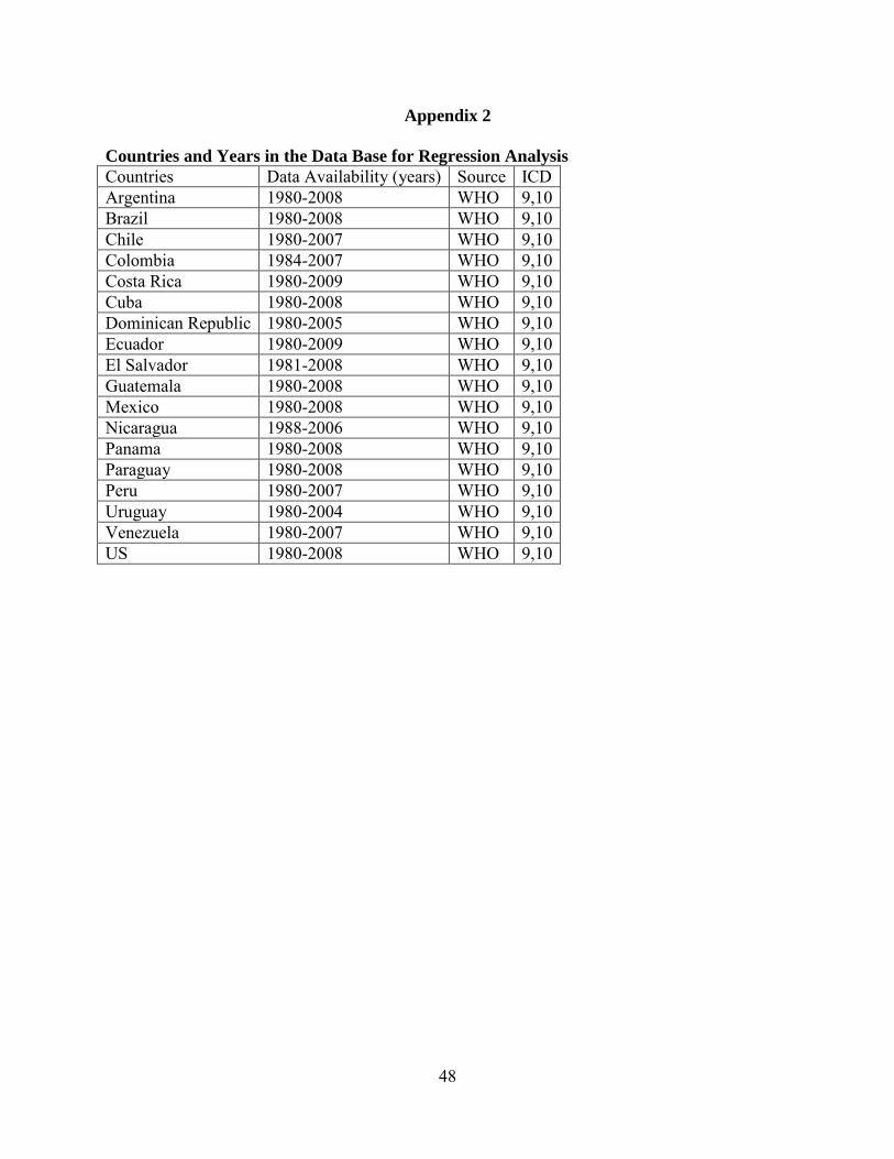
48

Appendix 2

Countries and Years in the Data Base for Regression Analysis

Countries Data Availability (years) Source ICD Argentina 1980-2008 WHO 9,10 Brazil 1980-2008 WHO 9,10 Chile 1980-2007 WHO 9,10 Colombia 1984-2007 WHO 9,10 Costa Rica 1980-2009 WHO 9,10 Cuba 1980-2008 WHO 9,10 Dominican Republic 1980-2005 WHO 9,10 Ecuador 1980-2009 WHO 9,10 El Salvador 1981-2008 WHO 9,10 Guatemala 1980-2008 WHO 9,10 Mexico 1980-2008 WHO 9,10 Nicaragua 1988-2006 WHO 9,10 Panama 1980-2008 WHO 9,10 Paraguay 1980-2008 WHO 9,10 Peru 1980-2007 WHO 9,10 Uruguay 1980-2004 WHO 9,10 Venezuela 1980-2007 WHO 9,10 US 1980-2008 WHO 9,10

49

Appendix 3

Differences between the Lee-Carter and Brass Logit models for lung cancer

The Brass logit model can be rewritten as follows:

H(x,t) = (t) + ((t)-1)* (ML

s(x))

= (t) + (t) * (MLs(x)) (A3.1)

where H(x,t) is the difference between the (logit-scaled) observed lung cancer mortality rates at age x and time t, ML(x,t), and the (logit-scaled) standard mortality rates, (ML

s(x)) The Lee-carter model can be rewritten in a similar way:

R(x,t) = K(t)* b(x) (A3.2) where R(x,t) is the difference between (log-scaled) observed lung cancer mortality rate at age x and time t and the average (log-scaled) lung cancer death rates observed during the period, A(x). Because the values of ML(x,t) are small, logit and log scaling yield virtually identical quantities. Thus, expressions (A3.1) and (A3.2) refer to approximately the same functions, particularly when in both cases we use the average observed rates to express the standard (either A(x) or ML

s(x). Because the functional form on the right hand side of expressions (A3.1) and (A3.2) are analogous, the first and higher derivatives with respect to age and time will have the same form in either case. In each model the partial derivatives with respect to age depend on a product of an age- (but not time) dependent term and a time- (but not age) dependent term. The same holds for the partial derivatives with respect to time. The models are mathematically equivalent: both require an ex-ante chosen standard; both include a term to capture shifts over time and across ages and in both cases the effects of time and age are multiplicative and separable. The key difference is that (A3.1) is estimated separately by period whereas (A3.2.) is estimated simultaneously over all periods. The inclusion of additional observations after the last, say T, will change estimates of parameters when (A3.2) but leave all those before T invariant if (A3.1) is used. (A3.1) requires extra parameters to model changes over time and across ages whereas (A3.2) is constrained to use the same parameters to accommodate extra variation whereas (A3.1.) use extra parameters that help separate the impact of changes in the total mortality level from impacts that are age-time specific. Such flexibility is absent in (A3.2) and this will explain is worse performance

Center for Demography and Ecology University of Wisconsin

1180 Observatory Drive Rm. 4412 Madison, WI 53706-1393

U.S.A. 608/262-2182

FAX 608/262-8400 comments to: palloni@ssc.wisc.edu requests to: cdepubs@ssc.wisc.edu