CEMARE Research Paper 154

A viability analysis for a bio-economic model

C Béné, L Doyen and D Gabay N.B. This research paper is an earlier version of Béné, C., Doyen, L. and Gabay, D. “A viability analysis for a bio-economic model” to be published in Ecological Economics 2001 No.36: 385-396 Abstracted and Indexed in: Aquatic Sciences and Fisheries Abstracts

Centre for the Economics and Management of Aquatic Resources (CEMARE), Department of Economics, University of Portsmouth, Locksway Road, Portsmouth PO4 8JF, United Kingdom. Copyright © University of Portsmouth, 2000 All rights reserved. No part of this paper may be reproduced, stored in a retrievable system or transmitted in any form by any means without written permission from the copyright holder.

ISSN 0966-792X

A Viability Analysis for a Bio-Economic Model

C. B�en�e�, L. Doyeny and D. Gabayz

Abstract: This paper presents a simple dynamic model dealing with the man-

agement of a renewable resource. But instead of studying the ecological and eco-

nomic interactions in terms of equilibrium or optimal control, we pay much at-

tention to the viability of the system or, in a symmetric way, to crisis situations.

These viability/crisis situations are de�ned by a set of economic and biological state

constraints. The analytical study focus on the compatibility between the state con-

straints and the controlled dynamics. Using the mathematical concept of viability

kernel, we reveal the situations and, if possible, management options to guaran-

tee a perennial system. Going further, we de�ne \overexploitation" indicators by

the time of crisis function. In particular, we point out irreversible overexploitation

con�gurations related to the resource extinction.

Key-words: renewable resource, bio-economic model, overexploitation,

viable control.

�CEMARE (Center for the Economics and Management of Aquatic Re-

sources), Locksway Road, Southsea Hants PO4 8JF, United Kingdom. E-mail:

christophe.bene@port.ac.ukyCNRS, Centre de Recherche Viabilit�e-Controle, Universit�e Paris-Dauphine, Place du

Mar�echal de Lattre de Tassigny, 75775 Paris cedex 16, France. Email: doyen@viab

.dauphine.frzCNRS, Centre de Recherche Viabilit�e-Controle, Universit�e Paris-Dauphine, Place

du Mar�echal de Lattre de Tassigny, 75775 Paris cedex 16, France. Email:

gabay@viab.dauphine.fr

1

1 Introduction

Economics of natural resources relies mainly on interactions between eco-

nomic and biological (or ecological) dynamics, which makes the problem

both interesting and di�cult. Over the past decades, the topic has re-

ceived growing attention because of the recent emergence of a common "en-

vironmental issue consciousness" and also because natural resource exploita-

tion has been shown to be characterized by very frequent "market failures"

(Pierce-Warford, 1993; Tisdell, 1991). This paper concentrates on the exam-

ple of marine renewable resources and their economic exploitation through

�sheries.

Most economic models addressing the problem of renewable resource

exploitation are built up on the frame of a biological model. Such mod-

els may account for the demographic structure (age or size classes) of the

exploited stock (trees, �sh population) or may attempt to deal with the

inter-species dimension of the exploited (eco)system. However, biologists

have often found it necessary to introduce various degrees of simpli�cations

to reduce the complexity of the analysis and one of the simplest models

used in population dynamics is the \logistic model". In such a model, the

stock, measured by its biomass, is considered globally, as one single unit,

without any consideration for the structure population, and its growth is

materialized through the logistic equation:

_x(t) =dx

dt(t) = rx(t)(1�

x(t)

l) = f(x(t));

where x(t) stands for the resource biomass, l is the limit carrying capacity

of the ecosystem and r is the intrinsic growth rate of the resource.

When �shing activities are included, the model becomes the Schaefer

(1954) model

_x(t) = f(x(t))� h(t);

where h(t) is the harvesting ow at time t. It is frequently assumed that the

catch rate h is proportional to both biomass and extraction e�ort, namely

h = qex, where e stands for the extraction e�ort (or �shing e�ort, an index

related for instance to the number of boats involved in the activity) and

q is a constant parameter usually referred as the catchability coe�cient.

At equilibrium, when the exploitation rate equals the population growth,

one obtains the so-called sustainable yield associated to the �shing e�ort by

inverting the relation

e =r

q(1�

x

l) = s(x):

2

The economic model which is directly derived from the Schaefer model

is the Gordon model (Gordon, 1954) which integrates the economic aspects

of the �shing activity through the �sh price p and the �shing costs c per

unit of e�ort. Assuming that the pro�t is de�ned by � = pqex� ce, one can

compute the e�ort e maximizing �. The Gordon model prediction, when

open access situation occurs (i.e. when no limitation is imposed on the

�shery's e�ort), is that the rent generated by the activity is dissipated as

the e�ort expands beyond e and the economy converges toward the so-called

\open access bionomic equilibrium".

Although it su�ers from a large number of unrealistic assumptions (some

of them ensuing directly from the Schaefer model limitations), the Gordon

model displays a certain degree of concordance with empirical �sheries his-

tories (Wilen, 1976). This is probably the reason why, along with its indis-

putable normative character, it has been regularly used as the underlying

framework by optimal control theory since the latter has been introduced

in �sheries sciences (see for instance Charles, 1983; Clark, 1976; Clark-

Kirkwood, 1979; Cohen, 1987; Goh, 1979; McKelvey, 1985).

In optimal control theory, assuming a �xed production structure (i.e.

constant capital and labor), the problem can be stated as the inter-temporal

maximization of the pro�t with respect to the �shing e�ort e(t)

maxe(�)

Z 1

0e��t(pqe(t)x(t)� ce(t))dt;

where � represents the social discount rate and x(�) is the solution of the

control system:(_x(t) = f(x(t))� qe(t)x(t); 0 � e(t) � emax

x(t) � 0:

with emax the e�ort limit resulting from the �xed production capacity (num-

ber of boats and of �shermen). Using the maximum principle, it can be

shown that the optimal strategy is to reach the steady state x? following

a \bang" (or most rapid) solution (c.f. Clark, 1976). Several extensions

have then been proposed to improve the realism of this basic model: for in-

stance accounting for the multi-species or multi-objectives that are known to

characterize most �shery systems (Charles, 1989; Diaz-Seijo, 1992; Healey,

1984); or integrating the irreversibility or the non-malleability of the capital

dynamics (Charles, 1989; Clark, 1976; Clark-Munro, 1975); or introducing

uncertainty (Charles, 1983; Clark-Kirkwood, 1986).

3

These various developments however did not prevent optimal control the-

ory to su�er criticisms regarding its applicability to �sheries management.

One has observed that �shermen' decisions are seldom driven by the search

for direct optimality (Bockstael, 1983; Hilborn-Ledbetter, 1979). In order to

maximize the objective function, one may also have in some cases to follow

optimal solutions that bring undesirable outcomes. Two typical examples of

these undesirable consequences are (i) negative pro�ts: the optimal strat-

egy requires to close the �shery for a while (which, practically, implies some

�xed costs not taken into account) and (ii) resource extinction: Clark (1973)

showed that it would be optimal to "liquidate" the resource and to re-invest

the capital in another activity when the resource growth rate is lower than

the discount rate.

Optimal control theory has not only been criticized for the outcomes

that it may bring about. It also su�ers some limitations inherent to the

optimization principle itself. On one hand, the optimal solution path is

generally unique which does not allow for possible alternate strategies. In

addition, it is strongly related to the choice of the discount factor �, which

is itself rather arbitrary.

All these remarks show the interest to address the problem from a dif-

ferent perspective attempting, in particular, at reconciling ecological and

economical issues. This is the way we choose in the present paper by look-

ing for some instantaneous and simultaneous \criteria" that materialize the

\good health" of the bio-economic system, i.e. its viability . The viability

approach (Aubin, 1991) deals with dynamic systems under state constraints

(see also Clarke et al, 1995). The aim of this method is to analyze the com-

patibility between the (possibly uncertain) dynamics of a system and state

constraints and to determine the set of controls (or decisions) than would

prevent this system from entering crises i.e. from violating its viability con-

straints. The present study is an attempt to apply this approach to the case

of the management of renewable resources and especially to �sheries. We

refer to B�en�e-Doyen (2000), Bonneuil (1994), Doyen et al. (1996) in others

contexts and to Toth et al (1998) for a similar approach untitled the Toler-

able Windows Approach. Here, we de�ne the viability from the viewpoint

of a government that aims at maintaining the �shery in a sustainable way.

To achieve this, a condition (or constraint) of net bene�ts (positive balance

sheets) of the �shing activity is imposed at any time on the resource and the

e�ort levels. Whenever one assumes some �xed costs, it appears that this

economic constraint induces a minimal threshold for the renewable resource

which is interesting if the government policy aims at reconciling ecological

4

and economics objectives. Then, using the mathematical concept of viabil-

ity kernel (Aubin, 1991), we make clear the need to anticipate the dynamics

of the system to maintain its viability. This analysis allows us to identify

situations of overexploitation and the adaptive regulations required to pre-

vent de�cits and/or overexploitation situations from occurring. A second

mathematical concept, the time of crisis function (Doyen-StPierre, 1997), is

then used to re�ne the overexploitation analysis. In particular, this over-

exploitation indicator allows us to identify two di�erent types of crises, the

reversible crises and the irreversible ones. It shows how the irreversible crisis

situations are linked to the resource extinction.

2 The model

2.1 The dynamics

The natural growth rate of the resource x is represented by a logistic law f

depending on the intrinsic growth parameter r > 0 and the limit capacity l

i.e.

f(x) = rx(1�x

l):

Taking into account that harvesting is proportional both to the biomass

x and to the �shing e�ort e, we consider the following dynamics for the

renewable resource

_x(t) = f(x(t))� qe(t)x(t);

where q stands for a catchability coe�cient.

We furthermore assume that the time variation of the e�ort is bounded:

_e(t) = u(t); u(t) 2 U = [u�; u+]: (1)

This assumption is a way to model the rigidity of the decision since it implies

the continuity of e�ort with respect to time and thus rules out jumps of

harvesting. For instance, it means that a decrease or an increase in number

of used boats requires time to be completed. We furthermore suppose that

u�� 0 � u

+ which means that the e�ort can be kept constant (case _e = 0).

We obtain the following control di�erential system where the state vari-

ables are (x; e) and the control variable is u:(_x(t) = f(x(t))� qe(t)x(t);

_e(t) = u(t); u�� u(t) � u

+:

(2)

5

2.2 The viability constraints

A second step is to express state variable constraints from a regulating (say

a government) agency viewpoint.

First, we impose an ecological constraint in the sense that the govern-

ment policy requires a minimum level xmin > 0 for the resource:

xmin � x(t); 8t � 0: (3)

The second constraint concerns the �shing e�ort e(t). We assume that cap-

ital and labor involved in the production process remain constant; therefore

e(t) is constrained by a �xed production capacity. We denote this limit

capacity emax and we thus identify a second constraint:

0 � e(t) � emax; 8t � 0: (4)

Furthermore, we consider that the government agency seeks to guarantee

the sustainability of the activity by maintaining a global positive net bene�t

in the sector at any time. Let us denote by R(x(t); e(t)) the sector balance

sheet, de�ned as the di�erence between the income and the harvesting costs.

Therefore the bene�t constraint reads as follows :

R(x(t); e(t)) = pqe(t)x(t)� ce(t)� C � 0; 8t � 0; (5)

where p > 0 represents the (exogenous) unit �sh price, c > 0 denotes the cost

per unit of e�ort and C > 0 is a �xed cost - which may include, for instance,

wages (assumed constant since labor is �xed) or a �xed amortization of the

capital stock (boats,..).

Note �rst that the net bene�t constraint (5) induces the resource biomass

to be strictly greater than c=pq, namely an ecological constraint. For sake

of simplicity, we assume that :

xmin �c

pq< l:

Note also that this same constraint (5) yields a strictly positive minimal

e�ort (and harvesting) since

e(t) �C

pqx(t)� c> 0:

This can be related, for instance, to an employment requirement. Thus one

can see this net bene�t constraint as a way to reconcile the ecological and

6

economic points of view. Notice also that constraint (5) materializes a dif-

ference between the viability approach and the optimal control approach.

In the optimal control approach, the value to optimize would be the inte-

gral over time of the discounted pro�tR10 e

��tR(x(t); e(t))dt. The optimal

solution1 may require the shutdown of the activity for a while (e(t) = 0)

which induces a negative balance for the period and thus leads to the viola-

tion of the constraint (5). Furthermore, we assign an equal weight to every

time period, thereby avoiding the discussion with respect to the choice of

the discount factor.

To summarize the viability constraints, we denote by K the constraint

(or target) set represented on �gure 1 and de�ned by

K = f(x; e) 2 IR2; 0 � e � emax; R(x; e) = pqex� ce� C � 0g: (6)

We shall say that a trajectory (x(:); e(:)) is viable in K if and only if we

have

(x(t); e(t)) 2 K; 8t � 0:

3 A viability analysis

A �rst question that arises now is to determine whether the evolution (2)

is compatible with the set of constraints K de�ned by (6). In other words,

we aim at revealing levels of resource and e�ort of the constraint domain

K that are associated with a viable trajectory in K and thus with a viable

regulation (open-loop) t ! u(t). To achieve this, we proceed in several

steps: identi�cation of viable stationary points, of viability niches, of the

viability kernel and computation of the viable regulations associated with

it. In order to restrict the mathematical content of the paper, we omit the

proofs of the di�erent results presented below; these proofs can be found in

B�en�e et al, 1998.

1At this stage, let us emphasize that viability and optimality are not exclusive ap-

proaches. Indeed, some optimal solution can be viable (in the sense we have just de�ned),

while some are not (according to the existence of a �xed cost). Furthermore, there are

several ways to reconcile optimal and viability approaches. One consists in solving the

inter-temporal optimality problem under the viability constraint. This means that the

economic motivations of the agents operating in the system could be to optimize the

inter-temporal pro�t under the positive pro�t constraint. Another direction is to consider

a myopic (non inter-temporal) viable optimization namely to �nd the feedback control(s)

that maximizes pro�t among the viable options (i.e in the so-called viable regulation map).

7

3.1 Viable stationary points

The �rst step of the analysis concerns the viable stationary points of the

system, which correspond to _x = 0; _e = 0. Because of the constraint

x(t) � xmin > 0, the solution x = 0 is clearly not a viable equilibrium. The

others solutions, referred as the \sustainable yield levels" in the classical

approach, are de�ned by:

e = s(x) =r

q(1�

x

l) and u = 0:

These equilibria are viable whenever (x; s(x)) 2 K. It can be shown (B�en�e

et al., 1998, Appendix A1) that:

Proposition 3.1 A necessary and su�cient condition for the existence of

viable equilibria for the system (2) is that8<: r � r� = 4pq2Cl

(pql�c)2

emax � e+ = r

2q (1�c+

p�

pql);

(7)

where

� = (pql + c)2 � 4pql(Cq

r+ c) = (pql � c)2 � 4

pq2lC

r:

In that case, the set of viable equilibria corresponds to the segment

EQ = f(x; e); e = s(x); max(x�; x�) � x � x

+g

de�ned by 8>><>>:x� = l

2 +c�

p�

2pq ;

x+ = l

2 +c+

p�

2pq ;

x� = s�1(emax):

Remark | The �rst condition (7) reveals a minimum intrinsic growth

rate value r� necessary to ensure the existence of a viable equilibria while

the second condition emphasizes the necessity of a minimum production

capacity e+ induced, in particular, by the occurrence of the �xed cost C.

These thresholds will play an important role for the computation of the

viability kernel. 2

8

3.2 Viability niches

As a second step of the analysis, we identify what we call the viability

niches. These viability niches correspond to initial resource level x(0) = x0

such that the resulting evolution, with a permanent policy e(t) = e0, remains

viable. They correspond to the most favorable situation since no regulation

is needed and the e�ort does not have to be changed to guarantee viability.

The niches N(e0) are thus de�ned by

N(e0) =

(x0

����� the solution (x(�); e0) of (2) with u(t) = 0;

starting from (x0; e0), is viable in K

):

Clearly, viable equilibria are part of viability niches. As illustrated on �gure

2, it turns out that the niches N(e0) exist whenever e0 2 [e+; e�] where wedenote by e

� the e�ort value

e� = s(x�) = r

2q (1�c�

p�

pql):

This requires condition (7) to hold. In the present case, the niches are

de�ned by

N(e0) = [( Ce0+ c)

pq;+1[:

3.3 Viability kernel and overexploitation

The next step is to study the whole viability of the system using the concept

of viability kernel. The viability kernel, denoted by Viab(K), corresponds

to the set of all initial conditions (x0; e0) such that there exists at least one

trajectory starting from (x0; e0) that stays in the set of constraints K. In

other words:

Viab(K) =

((x0; e0) 2 K

����� 9u(�) such that the solution (x(�); e(�)) of (2);

starting from (x0; e0), is viable in K

):

The viability kernel di�ers from the niches in that, for the kernel, regu-

lations through changes in e�ort can take place, thus allowing the viability

to be enlarged. To focus on over-exploitation issues, we assume that:

u+� max

x>x+ 0(x)(f(x)� q (x)x); (8)

9

where (x) = C

pqx�c. This condition (8) is related to the maximal rigidity

of e�ort and guarantee2 the possibility to increase su�ciently the e�ort for

high levels of resource and low levels of e�ort.

We can distinguish three qualitative con�gurations for the viability ker-

nel, depending mainly on the value of the resource parameter r. These three

cases are illustrated on Figure 3.

Case 1: Global viability (�gure 3(d)): The most favorable case takes

place when the viability kernel equals the whole set of constraints K, i.e.,

Viab(K) = K. This situation occurs mainly if the intrinsic growth rate r is

high enough (see proof in B�en�e et al., 1998, Appendix A3).

Proposition 3.2 If the conditions (7) and (8) hold true and if

emax � e� (9)

then,

Viab(K) = K;

namely, for every (x0; e0) 2 K, there exists a control u(:) such that the

solution (x(:); e(:)) of dynamics (2) starting from (x0; e0) is viable in K.

Remark | This statement means that whenever the e�ort emax is su�-

ciently low (still assuming that the second condition of (7) is not violated)

or, in a symmetric way, whenever the resource growth rate r is high enough,

viability holds everywhere and no over-exploitation occurs. In such a case,

every viable situation turns out to correspond to a viability niche and the

government agency does not need to regulate the �shery. In such a \sce-

nario", the maximal eet size is too moderate to induce any dangerous

mortality on the exploited resource. 2

Case 2: Partial viability (�gures 3(b-c)): The most signi�cant and

interesting case occurs when the viability kernel Viab(K) is a strict and

non-empty subset3 of K. This case occurs mainly when condition (9) does

not hold true i.e. emax > e�.

2This condition makes sense since it can be checked that maxx>x+

0(x)(f(x) �

q (x)x) < +13Namely Viab(K) � K with ; 6= Viab(K) and Viab(K) 6= K.

10

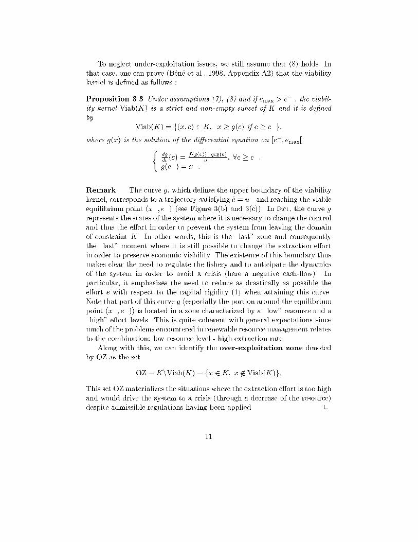
To neglect under-exploitation issues, we still assume that (8) holds. In

that case, one can prove (B�en�e et al., 1998, Appendix A2) that the viability

kernel is de�ned as follows :

Proposition 3.3 Under assumptions (7), (8) and if emax > e� , the viabil-

ity kernel Viab(K) is a strict and non-empty subset of K and it is de�ned

by

Viab(K) = f(x; e) 2 K; x � g(e) if e � e�g;

where g(x) is the solution of the di�erential equation on [e�; emax[(dg

de(e) =

f(g(e))�qeg(e)u�

; 8e � e�;

g(e�) = x�:

Remark | The curve g, which de�nes the upper boundary of the viability

kernel, corresponds to a trajectory satisfying _e = u� and reaching the viable

equilibrium point (x�; e�) (see Figure 3(b) and 3(c)). In fact, the curve g

represents the states of the system where it is necessary to change the control

and thus the e�ort in order to prevent the system from leaving the domain

of constraint K. In other words, this is the \last" zone and consequently

the \last" moment where it is still possible to change the extraction e�ort

in order to preserve economic viability. The existence of this boundary thus

makes clear the need to regulate the �shery and to anticipate the dynamics

of the system in order to avoid a crisis (here a negative cash- ow). In

particular, it emphasizes the need to reduce as drastically as possible the

e�ort e with respect to the capital rigidity (1) when attaining this curve.

Note that part of this curve g (especially the portion around the equilibrium

point (x�; e�)) is located in a zone characterized by a \low" resource and a

\high" e�ort levels. This is quite coherent with general expectations since

much of the problems encountered in renewable resource management relates

to the combination: low resource level - high extraction rate.

Along with this, we can identify the over-exploitation zone denoted

by OZ as the set

OZ = KnViab(K) = fx 2 K; x 62 Viab(K)g:

This set OZ materializes the situations where the extraction e�ort is too high

and would drive the system to a crisis (through a decrease of the resource)

despite admissible regulations having been applied. 2

11

Case 3: No viability (�gure 3(a)): It turns out that the viability kernel is

empty whenever condition (7) related to the existence of a viable equilibrium

is not satis�ed. Indeed, an equilibrium located in K is always a state of the

viability kernel.

Proposition 3.4 If condition (7) is not satis�ed, then Viab(K) = ;.

Remark | In particular, this means that, if the intrinsic growth rate value

r is smaller than the threshold r� de�ned in (7), then the system is not

sustainable; in other words, we face an overexploitation situation in every

case, i.e. OZ = K. 2

3.4 Viable regulations: how to avoid over-exploitation.

The viability kernel revealed the states biomass-e�ort compatible with the

constraints. The present step is to compute the viable management options

(decision or control) associated with it. For this purpose, we introduce the

viable regulation map U(x; e) which represents the controls u = _e that can

maintain viability for a state (x; e). For any point (x; e) in the viability

kernel Viab(K), we know that this regulation set is not empty. We consider

the case of partial viability, namely

Viab(K) = f(x; e) 2 K; x � g(e) if e � e�g:

Under the assumptions (7) and (8), we can prove (B�en�e et al., 1998, Ap-

pendix A4) that U(x; e) is then de�ned by:

U(x; e) =

8>>>>><>>>>>:

0 if e = e�; x = x

�

u� if x = g(e); e� < e � emax

[u�; 0] if x > g(e); e = emax

[�(x); u+] if R(x; e) = 0; x > x�

[u�; u+] otherwise,

where �(x) = max(u�; 0(x)(f(x)� q (x)x)).

Remark | From the calculation of this regulation map U , it appears that

the only mandatory unique regulation occurs when the anticipation of a

pro�t crisis is required i.e., when x = g(e). In that case, the choice in U(x; e)

reduces to u�. For any other situations within the viability kernel, several

12

viable regulations and viable policies are possible. This means that policy-

makers are o�ered di�erent viable alternatives which extends their exibility

with respect to the multiple, evolving (or sometimes con icting) objectives

they attempt to achieve. This result may represent an improvement with

respect to others approaches where only one solution is usually proposed. 2

4 Time of crisis and irreversibility.

In this section, we go a step further in the analysis of the system viability by

using the concept of time of crisis (Doyen-StPierre, 1997). We have pointed

out above the possible existence of an \overexploitation" area OZ where

the dynamics leads the system to leave the domain of constraints and in

particular to violate the bene�t constraint. Negative pro�ts happen in lots of

�sheries (at least for some �nite period) everywhere in the world. Indeed it is

not unusual that �shermen have to face periods where the value of the catch

does not cover the total operating costs. However these negative cash- ows

do not necessarily induce the de�nitive shutdown of the activity provided

that they do not last for too long. Consequently it is relevant to determine

what would happen in this situation, to evaluate the corresponding level of

overexploitation and, in particular, to study its irreversibility feature. So,

for a given trajectory (x(:); e(:)), we measure4 the length of the period of

negative pro�t (t; R(x(t); e(t)) < 0). Then, we compute the minimal length

of cash- ow crisis:

V (x; e) = infx(�);e(:);u(�)

measure(t; R(x(t); e(t)) < 0);

under the conditions8><>:x(�); e(:); u(�) solution of system (2)

x(0) = x; e(0) = e;

(x(t); e(t)) 2 H

4The measure is taken in the sense of

measure(t; R(x(t); e(t)) < 0) =

Zft�0 j R(x(t);e(t))<0g

dt:

13

where H (H � K) stands for the subset of constraints consisting simply of

the ecological minimal threshold and the maximal e�ort capacity as follows

H = f(x; e) 2 IR2; xmin � x; 0 � e � emaxg:

The crisis function V provides an indicator of overexploitation and shows

that three qualitative areas can be distinguished:

� No overexploitation: V (x; e) = 0. Inside the viability kernel Viab(K),

the value V (x; e) equals 0. This emphasizes again the existence of a

viable control and a solution that does not violate the state constraints

K. This case has already been fully discussed above.

� Reversible overexploitation: 0 < V (x; e) < +1: The overex-

ploitation crisis (x; e) 2 OZ = KnViab(K) can be solved in �nite

time. As illustrated in Figure 4, the cash ow crisis (R < 0) can be

long, and there is a period of time during which, even with a drastic

reduction of the activity ( _e = u�), the resource level will continue to

decrease until it reaches a level where it can be rebuilt. In that case,

the strategy is then to let the resource grow thanks to a \weak" e�ort

in order to return into the viability kernel.

� Irreversible overexploitation: V (x; e) = +1. The crisis (R < 0)

induced by the overexploitation becomes an irreversible crisis since it

leads to the \extinction" (x < xmin) of the resource and therefore to

the de�nitive shutdown of the economic activity. From Figure 4, it

appears that this situation may happen if the e�ort level is set high.

But it can also happen, in moderate harvesting e�ort situations, when

the change in strategy is decided too late i.e. when the pro�t R(x; e)

becomes negative. This can occur for instance if �shermen behaviors

are completely rigid: the reduction of e�ort is not applied (u = 0)

until the direct feasibility (to be in K) is at stake. In that case, if

one starts above the viability curve g, the resource decreases until one

reaches a point (bx; e0) where the viability is at stake (R(bx; e0) = 0).

If V (bx; e0) = +1, then, whatever the later change of strategy and

regulation, the resource and thus the economic activity will collapse.

5 Conclusion

In this study, we have addressed the problem of the management of natu-

ral resource exploitation systems. We re-visit the classical dynamic �shery

14

model within a new framework based on the concept of viability. The main

purpose of this new approach is not to maximize an objective function, but

to analyze the compatibility between the dynamics of the system and its

constraints and to determine the set of controls (or decisions) that prevent

the system from violating these viability constraints.

In the present case of a �shery model, management options are identi-

�ed, assuming a deterministic dynamics (no uncertainty) and a net bene�t

constraint with �xed cost. This bene�t constraint induces e�ort and biomass

minimal thresholds and thus aims at reconciling ecological and economics

requirements. The viability kernel analysis highlights the need to anticipate

the system dynamics to prevent sector de�cits that we relate with overex-

ploitation issues. Then, using the time of crisis concept, we evaluate di�erent

types of overexploitation. In particular, we distinguish a reversible overex-

ploitation zone, where the system can recover from crisis and come back

into the viable domain in �nite time, and an irreversible overexploitation

situation which leads to the extinction of the resource and to the de�nitive

shutdown of the activity.

It is clear that the model adopted in this study is quite stylized and built

up on simplistic assumptions. Future research is needed to relax some of

these assumptions. In particular, we aim at including resource uncertainties,

capital dynamics through investment, price dynamics and market demand

to make the model more realistic. We also hope to incorporate and analyze

behavior mechanisms such as cooperation with respect to the resource access

issue. More generally, the viability approach may provide an interesting

analytical framework to address some of the issues encountered in natural

resource management and sustainable development.

References

Aubin, J.P., 1991. Viability Theory. Birkh�auser, Springer Verlag.

B�en�e, C., 1997. Dynamics and adaptation of a �shery system to eco-

logical and economic perturbations: Analysis and dynamic modeling, The

French Guyana shrimp �shery case. Ph.D. Dissertation, University of Paris

VI, Paris, manuscript in French, 236 p.

B�en�e, C., and Doyen, L., 2000. Storage and Viability of a Fishery with

Resource and Market Dephased Seasonnalities. Journal of Environmental

Resource Economics, 15, pp 1-26.

15

B�en�e, C., Doyen, L. & Gabay, D., 1998. A Viability Analysis for a Bio-

economic model. Cahiers du Centre de Recherche Viabilit�e-Jeux-Controle,

N 9815.

Bockstael, N.E., and Opaluch, J., 1983. Discrete modeling of behavioral

response under uncertainty: the case of the �shery. J. Environ. Econ.

Manag., 10, pp 125-137.

Bonneuil N., 1994. Capital accumulation, inertia of consumption and

norms of reproduction, Journal of Population Economics, 7, pp 49-62.

Charles, A.T., 1983. Optimal Fisheries Investment under Uncertainty.

Can. J. Fish. Aquat. Sci., 40, pp 2080-2091.

Charles, A.T., 1989. Bio-socio-economic �shery models: labor dynamics

and multi-objective management. Can. J. Fish. Aquat. Sci. 46, pp. 1313-

1322.

Clark, C.W., 1973. The economics of overexploitation. Science, 181, pp.

630-634.

Clark, C.W., 1976. Mathematical Bio-economics: The Optimal Man-

agement of Renewable Resource. J. Wiley & Sons, New York.

Clark, C.W., and Kirkwood, G.P., 1979. Bioeconomic model of the Gulf

of Carpentaria prawn �shery. J. Fish. Res. Board Can., 36, pp. 1303-1312.

Clark, C.W., and Kirkwood, G.P., 1986. On Uncertain Renewable Re-

source Stocks: Optimal Harvest Policies and the Value of Stock Surveys.

Journal of Environmental Economics and Management, 13, pp. 235-244.

Clark, C.W., and Munro, G.R., 1975. The Economics of Fishing and

Modern Capital Theory: a Simpli�ed Approach. Journal of Environmental

Economics and Management, 2, 92-106.

Clarke, F.H., Ledyaev, Y.S., Stern, R.J., and Wolenski, P.R., 1995.

Qualitative properties of trajectories of control systems: a survey. J. of

Dynamical Control Systems, Vol 1, pp 1-48.

Cohen, Y., 1987. A review of harvest theory and applications of optimal

control theory in �sheries management. Can J. Fish. Aquat. Sci., 44 (suppl.

2)pp. 75-83.

Dasgupta, P., 1982. The Control of Resources. Basil Blackwell, Oxford.

Diaz-de-Leon, A., and Seijo, J.C., 1992. A multi-criteria non-linear op-

16

timization model for the control and management of a tropical �shery. Mar.

Resour. Econ., 7, pp. 23-40.

Doyen, L., and Saint-Pierre, P., 1997. Scale of Viability and Minimal

Time of Crisis. Journal of Set-Valued Analysis, 5: 227-246.

Doyen, L., Gabay, D., and Hourcade, J.C., 1996. Risque climatique,

technologie et viabilit�e. Actes des Journ�ees du Programme Environnement

Vie et Soci�et�es, CNRS, Session B, pp 129-134.

Goh, B.S., 1979. The usefulness of optimal control theory to biological

problem. In Theoretical Systems Ecology; Advances and Case Studies. E.

Halfon Ed., 385-399, Academic Press, New-York.

Gordon, H.S., 1954. The economic theory of a common property re-

source: the �shery. J. Pol. Econ., 82, 124-142.

Hartwick, J.M., and Olewiler, N.D., 1998. The Economics of Natural

Resource Use, second edition. Harper and Row, New York.

Healey, M.C., 1984. Multi-attribute analysis and the concept of optimal

yield. Can J. Fish. Aquat. Sci., 41, pp. 1393-1406.

Hilborn, R., and Ledbetter, M., 1979. Analysis of the British Columbia

salmon purse-seine eet: dynamics of movement. J. Res. Board Can., 36,

pp. 384-391.

Lauck, T., Clark, C.W., Mangel, M., and Munro, G.R., 1998. Imple-

menting the Precautionary Principle in Fisheries Management through Ma-

rine Reserves. Ecological Applications, 81 Special Issue. S72-78.

McKelvey, R., 1985. Decentralized Regulation of a Common Property

Renewable Resource Industry with Irreversible Investment. Journal of En-

vironmental Economics and Management, 12, pp 287-307.

Pierce, D.W., and Warford, J., 1993. World without end. World Bank,

Oxford University Press, 440 pp.

Schaefer, M.B., 1954. Some aspects of the dynamics of populations.

Bull. Inter. Amer. Trop. Tuna Comm., 1, pp. 26-56.

Tisdell, C.A., 1991. Economics of Environmental Conservation. Else-

vier, Amsterdam, 233 pp.

Toth, F.L., Bruckner, Th., Fussel, H.-M., Leimbach, M., Petschell-Held,

G., Schellnhuber, H.J., 1997. The tolerable windows approach to integrated

17

assessments. Proceedings of the IPCC Asia-Paci�c Workshop on Integrated

Assessment Models, Tokyo, Japan, 10-12th March 19.

Vedeld P.O., 1994. The environment and interdisciplinarity, Ecological

Economics (10)1, pp. 1-13.

Wilen, J.E, 1976. Common property resources and the dynamics of

over-exploitation: the case of the North Paci�c fur seal. Department of

Economics, Research Paper No.3, University of British Columbia, Vancou-

ver, Canada.

Wilen, J.E., 1993. Bioeconomics of renewable resource use. Handbook

of natural resource and energy economics, vol I, Part 1, Chapter 2, pp 61-

121, Edited by A.V. Kneese and J.L. Sweeney, Elsevier Science Publishers

B.V..

18

Figure 1: In grey, the domain of viability constraints K delimited by the

two constraints 0 � R(x; e) and e � emax.

19

Figure 2: In white, the viability niches.

20

(a) No Viability (b) Partial Viability

(c) Partial Viability (d) Global Viability

Figure 3: Viability kernels for di�erent values of the parameter r. In

white, the viability kernel Viab(K), in grey the overexploitation zone,

OZ = KnViab(K).

21

(a) Level curves of the minimal time crisis function.

(b) Graph of the minimal time crisis function. The grey area indi-

cates in�nite time crisis i.e., irreversible overexploitation situations.

The black area stands for the viability kernel.

Figure 4: Approximation of the crisis function V (x; e).

22