Cellular Viability Imaging Using Dynamic Light Scattering

Cellular Viability Imaging Using Dynamic Light

Scattering Optical Coherence Tomography

by

Julia Seungmi Lee

B.S. Mechanical Engineering and Industrial Engineering,

Korea University; Seoul, Korea, 2010

M.S. Mechanical Engineering, Korea University; Seoul, South Korea, 2012

M.S. Engineering, Brown University; Providence, RI, 2014

A dissertation submitted in partial fulfillment of the

requirements for the degree of Doctor of Philosophy

in the School of Engineering at Brown University

PROVIDENCE, RHODE ISLAND

May 2018

© Copyright 2018 by Julia Seungmi Lee

iii

This dissertation by Julia Seungmi Lee is accepted in its present form

by the School of Engineering as satisfying the

dissertation requirement for the degree of Doctor of Philosophy.

Date_____________

_________________________________________ Jonghwan Lee, Ph.D., Advisor

Recommended to the Graduate Council

Date_____________

Date_____________

_________________________________________ Diane Hoffman-Kim., Ph.D., Reader __________________________________________ Thomas R. Powers, Ph.D., Reader

Approved by the Graduate Council

Date_____________

___________________________________________ Andrew G. Campbell, Dean of the Graduate School

iv

Vitae

Julia Lee, after graduating from Daewon Foreign Language High School, attended Korea

University in Seoul, Korea, from which she graduated with a Bachelor of Science in

Mechanical Engineering and Industrial Engineering in 2010, then a Master of Science in

Mechanical Engineering in 2012. She completed her doctorate in engineering at Brown

University in 2018, collecting a Master of Science in Engineering in 2014 en route.

v

Acknowledgement

First and foremost, I would like to express my deep gratitude to my advisor, Jonghwan Lee,

for his guidance and support. Thanks to all the members in Lee lab, with special thanks to

Kyungsik Eom, Collin Polucha, and Madison Kuhn for help during the experiments; to our

collaborators in Morgan Lab, with special thanks to Blanche Ip, Ben Wilks, and Kali

Manning for providing samples; to Dr. Jefferey Morgan for guidance in delivering my

research to the audiences.

Deep gratitude and love to my friends and family.

vi

To my family and family-to-be

vii

Abstract of Cellular Viability Imaging Using Dynamic Light Scattering Optical

Coherence Tomography, by Julia Seungmi Lee, Ph.D., Brown University, May 2018.

Cellular viability represents whether a cell is performing normal functions, relating to

intracellular energy synthesis. Accurately quantifying the cellular viability would facilitate

novel studies on how pathological environments affect the functioning of cells in various

diseases. Nevertheless, technologies for monitoring the cellular viability in live tissue

models are currently lacking. This study aims at testing a recently developed technology,

which integrates dynamic light scattering and optical coherence tomography (called DLS-

OCT), to image the cellular viability with single-cell resolution. DLS analyzes fluctuations

in light scattered by particles to measure diffusion or flow of the particles, and OCT uses

coherence gating to collect light only scattered from a small volume for high-resolution

structural imaging. Integrating the two technologies, DLS-OCT constructs high-resolution

diffusion coefficient and flow velocity 3D maps. It is known that the motion of intracellular

organelles, often called intracellular motility, resembles a random walk in the confined

cytoplasm space, thus it can be quantified by the diffusion coefficient. Since the

intracellular motility is correlated with the cell’s metabolism level, the diffusion coefficient

map of DLS-OCT is expected to enable us to image the cellular viability. Here, the DLS-

OCT imaging of cellular viability was validated by characterizing responses of the

measured intracellular motility to the environmental conditions such as the temperature

and pH, in animal retinal explant samples. First, we characterized our new OCT system

and optimized scanning sequences and processing procedures for DLS-OCT data, to match

the dynamic range of our DLS-OCT measurement with the typical range of intracellular

viii

motility. Both numerical simulation and phantom experiments were performed for

optimization. Second, methods required for animal retinal explant experiments were

established, and DLS-OCT data from retinal tissue while manipulating the cellular viability

were acquired and analyzed, to test the technical hypothesis that DLS-OCT-measured

intracellular motility of neurons significantly diminishes when the cellular viability levels

are out of the physiological ranges. Similar operations were performed to tissue spheroids

with additional morphological measurements. As a result, we measured individual cells’

healthiness for tempered conditions, which will enlighten studying cells’ healthiness

during disease progress or therapeutic treatment in stroke, epilepsy, and Alzheimer’s

disease among others.

ix

Contents

1........................................................................................................................................... 1

INTRODUCTION .............................................................................................................. 1

1.1. Biological Background ......................................................................................... 2

Cellular Structures ........................................................................................ 2

Cellular Metabolism...................................................................................... 3

Intracellular Motility ..................................................................................... 6

Effects of Environmental Change and Chemical Treatment on Intracellular Motility ....................................................................................................................... 7

1.2. Technical Background.......................................................................................... 8

Previous Techniques to Measure Intracellular Motility................................ 8

Previous Techniques to Measure Intracellular Diffusion Coefficient ........ 10

1.3. Objective and strategy ........................................................................................ 13

Previous studies with OCT to measure dynamics....................................... 14

2......................................................................................................................................... 15

DYNAMIC LIGHT SCATTERING OPTICAL COHERENCE TOMOGRAPHY ........ 15

2.1. Introduction ........................................................................................................ 16

2.2. Theoretical background ...................................................................................... 17

Optical Coherence Tomography ................................................................. 17

Dynamic Light Scattering ........................................................................... 20

Dynamic Light Scattering Optical Coherence Tomography (DLS-OCT) .. 21

2.3. DLS-OCT simulation ......................................................................................... 24

Motivation for Simulation........................................................................... 24

Procedures of Simulation ............................................................................ 25

Simulation Results ...................................................................................... 25

Discussion on Numerical Simulation.......................................................... 28

2.4. Experimental setup ............................................................................................. 30

Spectral-Domain Optical Coherence Tomography (SD-OCT) System ...... 30

DLS-OCT .................................................................................................... 31

Simultaneous fluorescence imaging ........................................................... 32

Data Acquisition and Processing ................................................................ 33

2.5. Results and discussions ...................................................................................... 35

x

Characterization of the System ................................................................... 35

Phantom measurement of diffusion coefficient .......................................... 38

Simultaneous OCT and fluorescence imaging ............................................ 41

3......................................................................................................................................... 44

CELLULAR VIABILITY MEASUREMENT OF RETINAL NEURONAL CELLS.... 44

3.1. Introduction ........................................................................................................ 45

3.2. Experimental methods ........................................................................................ 46

Retinal dissection and handling .................................................................. 46

Image acquisition ........................................................................................ 48

Drug induce and temperature change ......................................................... 53


Fluorescence imaging ................................................................................. 54

Diffusion coefficient ................................................................................... 55

Decorrelation............................................................................................... 68

3.4. Conclusions ........................................................................................................ 80

4......................................................................................................................................... 81

CELLULAR VIABILITY MEASUREMENT OF TISSUE SPHEROIDS...................... 81

4.1. Introduction ........................................................................................................ 82

Fibroblast .................................................................................................... 83

HEP G2 ....................................................................................................... 84

4.2. Experimental methods ........................................................................................ 84

Microscopic imaging .................................................................................. 84

Macroscopic imaging .................................................................................. 84


Viability metric observations ...................................................................... 93

Morphological observations........................................................................ 99

4.4. Conclusions ...................................................................................................... 110

5....................................................................................................................................... 112

CONCLUSION ............................................................................................................... 112

xi

List of Tables

Table 1 Effect of environmental change and chemical treatment on the cell ......................7

Table 2 Previous methods to measure intracellular motion .................................................9

Table 3 Previous methods to measure diffusion coefficient ..............................................12

xii

List of Figures

Figure 1 Cellular structure. ..................................................................................................3

Figure 2 Schematics of interferometers. (a) Schematic of Michelson interferometer. (b)

Schematic of time-domain optical coherence tomography. ...............................................18

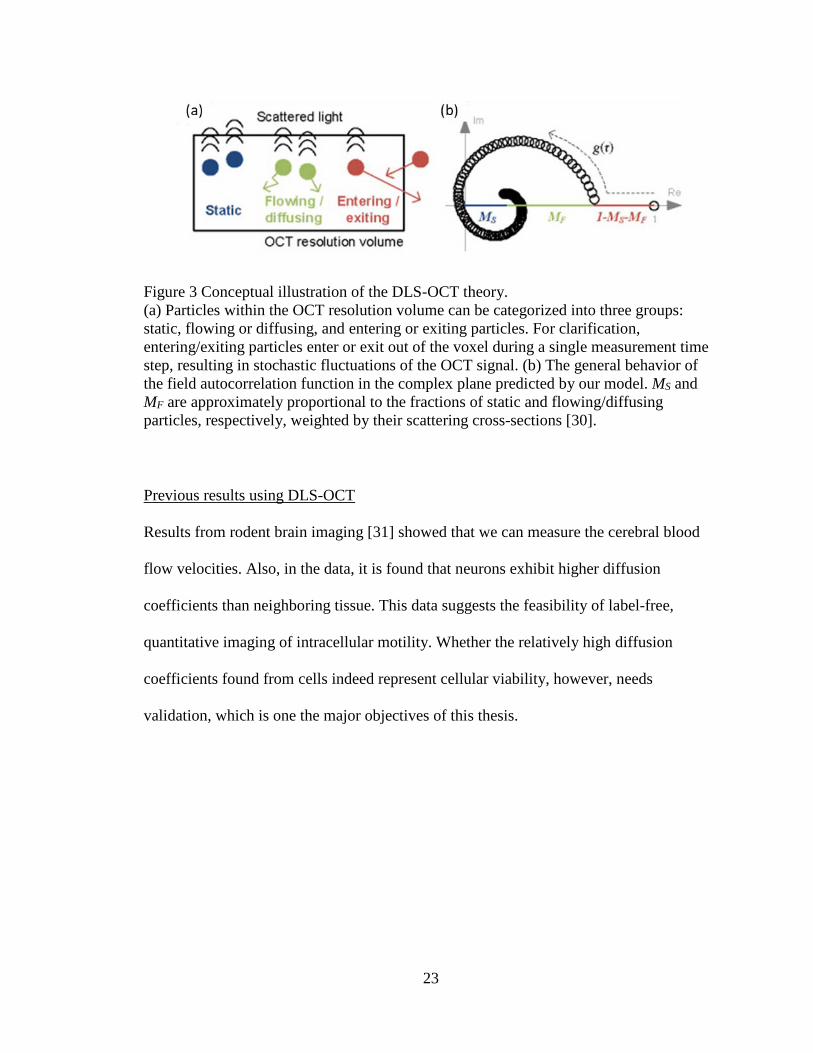
Figure 3 Conceptual illustration of the DLS-OCT theory. (a) Particles within the OCT

resolution volume can be categorized into three groups: static, flowing or diffusing, and

entering or exiting particles. For clarification, entering/exiting particles enter or exit out of

the voxel during a single measurement time step, resulting in stochastic fluctuations of the

OCT signal. (b) The general behavior of the field autocorrelation function in the complex

plane predicted by our model. MS and MF are approximately proportional to the fractions

of static and flowing/diffusing particles, respectively, weighted by their scattering cross-

sections [30]. ......................................................................................................................23

Figure 4 Process of numerical simulation for validating the DLS-OCT theory. True values

of the diffusion coefficient and velocity were determined by fitting the mean square

displacement (MSD) of the numerical position data. ........................................................25

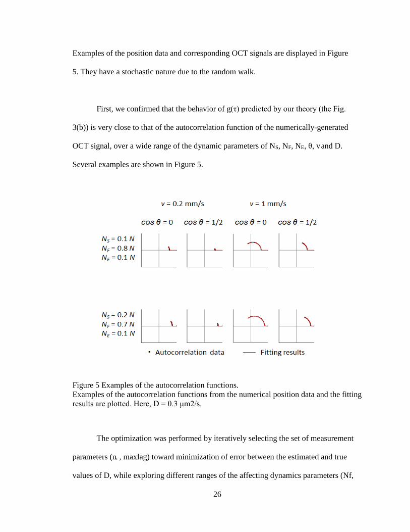
Figure 5 Examples of the autocorrelation functions. Examples of the autocorrelation

functions from the numerical position data and the fitting results are plotted. Here, D = 0.3

μm2/s. .................................................................................................................................26

Figure 6 Results of numerical DLS-OCT measurements. Results of numerical DLS-OCT

measurements with the optimum measurement parameters (nt, τmax) and over the

appropriate ranges of the dynamics parameters (Nf and v). The performance was tested for

a total of 1,050 combinations (6 number densities, 5 diffusion coefficients, 5 velocities and

xiii

7 flow angles). ME= 1 - MS - MF. The points represent the mean and error from other

combinations, while fixing the parameter of investigation. ...............................................27

Figure 7 The error in measurements of D and MF·D. (a) D (b) MfD over the whole range

(c) Magnified view of the box in (b). .................................................................................28

Figure 8 Examples of the autocorrelation functions with conventional theory. Examples of

the autocorrelation functions of the numerical OCT data of the conventional theory. Here,

v = 1 mm/s, and vz = 0 mm/s. ............................................................................................29

Figure 9 Examples of the autocorrelation functions with our new theory. Examples of the

autocorrelation functions of the numerical OCT data follows our new theory than the

conventional one. Here, v = 0.1 mm/s, and vz = 0 mm/s. ..................................................30

Figure 10 Schematic of simultaneous imaging system. .....................................................33

Figure 11 Lateral resolution calculation using Rayleigh Criterion. (a) Maximum intensity

projection of the 3D volume (1024 pixels X 512 pixels X 512 pixels) image from SD-OCT

signal. (b) Magnified view of the area of interest marked in (a). (c) The intensity of the

white line in (b). .................................................................................................................37

Figure 12 Normalized intensity plot of USAF target. Normalized intensity plot of USAF

target per line width with Rayleigh criterion as a comparison (Line). ..............................38

Figure 13 Static sample measurement. Diffusion coefficient, velocity, and coefficient of

determination for the static sample measurement with the optimal fitting condition. .......39

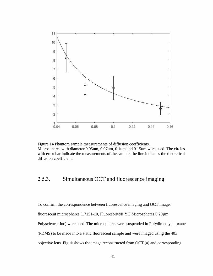
Figure 14 Phantom sample measurements of diffusion coefficients. Microspheres with

diameter 0.05um, 0.07um, 0.1um and 0.15um were used. The circles with error bar indicate

the measurements of the sample, the line indicates the theoretical diffusion coefficient. .41

xiv

Figure 15 Simultaneous imaging of fluorescent microbeads. Acquired image of fluorescent

microbeads from OCT signal (a) and fluorescence imaging (b) using 40x lens. Red arrows

indicate the corresponding figures in both images. ...........................................................42

Figure 16 Images of 1951 USAF target. Images of 1951 USAF target from OCT signal (a)

and OCT camera (b) using 40x lens. White dotted circles indicate the corresponding area.

............................................................................................................................................43

Figure 17 Dark box setup for image acquisition. Retina imaging chamber is located below

SD-OCT for image acquisition. SD-OCT system and the retina chamber are inside a dark

box......................................................................................................................................49

Figure 18 Retina imaging chamber. (a) Assembled retina imaging chamber and filter holder

design in Solidworks. (b) 3D-printed product of the model attached to the breadboard. The

image shows the needles used for perfusion supply system. .............................................50

Figure 19 Schematic of the retina chamber. The perfusion medium bubbled with Oxygen

with 5% CO2 then travels through the heater to be supplied to the retina chamber. Waste

medium is sucked with vacuum on the other end of the chamber. ....................................51

Figure 20 Comparison of cell images in fluorescence imaging and SD-OCT imaging. ...55

Figure 21 Baseline measurement of diffusion coefficient. ................................................56

Figure 22 Diffusion coefficient of the retinal neural cells to different temperatures.. ......57

Figure 24 Diffusion coefficient of the retinal neural cells to exposure of 2.2M of ethanol in

the media. ...........................................................................................................................59

Figure 25 Diffusion coefficient of the retinal neural cells to exposure of hypotonic

condition.. ..........................................................................................................................61

xv

Figure 26 Diffusion coefficient of the retinal neural cells to exposure of hypertonic

condition. ...........................................................................................................................62

Figure 27 Diffusion coefficient of the retinal neural cells to exposure of pH 8. ...............64

Figure 28 Diffusion coefficient of the retinal neural cells to exposure of pH 3.5. ............65

Figure 29 Comparison of diffusion coefficient of the retinal neural cells to the pilocarpine.

............................................................................................................................................67

Figure 30 Intensity, decorrelation, and relative decorrelation maps. .................................69

Figure 31 Decorrelation response to different temperatures ..............................................71

Figure 32 Decorrelation response to ethanol .....................................................................73

Figure 33 Decorrelation response to osmolarity ................................................................75

Figure 34 Decorrelation response to pH ............................................................................77

Figure 35 Decorrelation response to pilocarpine ...............................................................79

Figure 36 Maximum intensity projections of tissue spheroid inside. ................................86

Figure 37 Maximum intensity projections of HEP G2 spheroids .....................................87

Figure 38 Binary image after thresholding ........................................................................88

Figure 39 Mask array .........................................................................................................89

Figure 40 Post -mask array ................................................................................................90

Figure 41 Maximum intensity projection of tissue array in final form..............................91

Figure 42 En face images of the differential array. ...........................................................92

Figure 43 Maximum intensity projection of tissue array where a spheroid is selected. ....92

Figure 44 Maximum intensity projection of individual spheroids ....................................94

Figure 45 Intensity, decorrelation, and relative decorrelation at 14 pixels (48.44 um) below

the tissue equator................................................................................................................95

xvi

Figure 46 Intensity, decorrelation, and relative decorrelation at the tissue equator. .........96

Figure 47 Maximum intensity projection of individual spheroids with different seeding

numbers in yz plane. ..........................................................................................................97


numbers in yz plane. ..........................................................................................................98

Figure 49 Maximum projections of intensity, decorrelation, and relative decorrelation at

the surface of the tissue and at 6 pixels (20.76 um) below the tissue surface. ..................99


numbers in xy and yz planes. ...........................................................................................100

Figure 51 Maximum intensity projection of individual spheroids with different DIV in xy

and xz planes. ...................................................................................................................101

Figure 52 Surface area to volume ratio with error bars ...................................................102

Figure 53 Height to width ratio (HWR) to seeding numbers.. .........................................103

Figure 54 Tissue volume plotted to seeding numbers.. ...................................................104

Figure 55 Cellular volume (volume of a cell) is plotted to seeding numbers. .................105


numbers in xy and yz planes. ...........................................................................................106

Figure 57 Surface area to volume ratio with error bars of samples to the seeding numbers.

..........................................................................................................................................107

Figure 58 Height to width ratio (HWR) to seeding numbers. ..........................................108

Figure 59 Tissue volume (mm3) is plotted to seeding numbers.. .....................................109

Figure 60 Cellular volume (mm3, volume of a cell) is plotted to seeding numbers. .......110

1

1.

INTRODUCTION

2

1.1. Biological Background

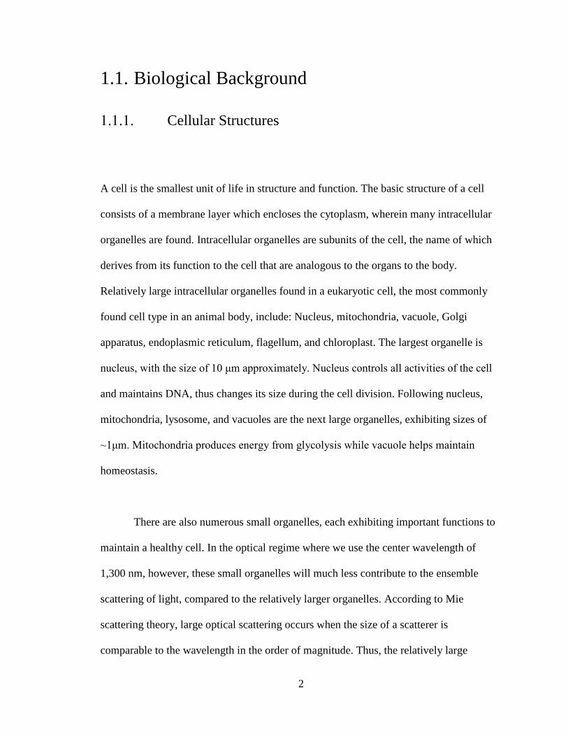
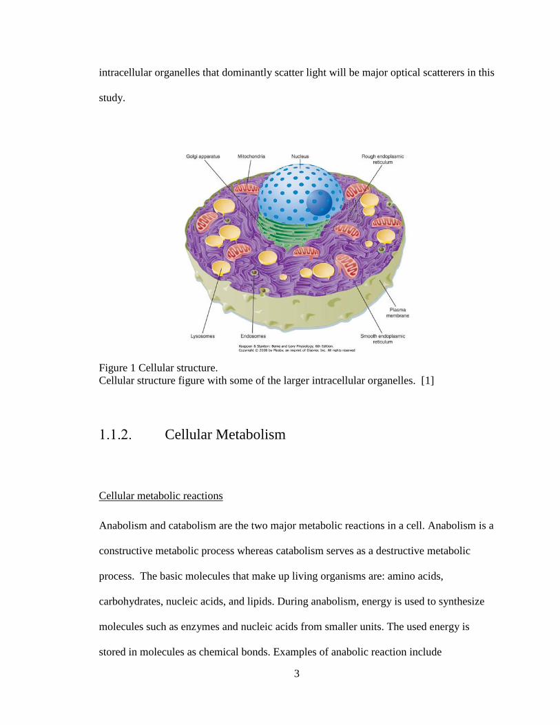
Cellular Structures

A cell is the smallest unit of life in structure and function. The basic structure of a cell

consists of a membrane layer which encloses the cytoplasm, wherein many intracellular

organelles are found. Intracellular organelles are subunits of the cell, the name of which

derives from its function to the cell that are analogous to the organs to the body.

Relatively large intracellular organelles found in a eukaryotic cell, the most commonly

found cell type in an animal body, include: Nucleus, mitochondria, vacuole, Golgi

apparatus, endoplasmic reticulum, flagellum, and chloroplast. The largest organelle is

nucleus, with the size of 10 μm approximately. Nucleus controls all activities of the cell

and maintains DNA, thus changes its size during the cell division. Following nucleus,

mitochondria, lysosome, and vacuoles are the next large organelles, exhibiting sizes of

~1μm. Mitochondria produces energy from glycolysis while vacuole helps maintain

homeostasis.

There are also numerous small organelles, each exhibiting important functions to

maintain a healthy cell. In the optical regime where we use the center wavelength of

1,300 nm, however, these small organelles will much less contribute to the ensemble

scattering of light, compared to the relatively larger organelles. According to Mie

scattering theory, large optical scattering occurs when the size of a scatterer is

comparable to the wavelength in the order of magnitude. Thus, the relatively large

3

intracellular organelles that dominantly scatter light will be major optical scatterers in this

study.

Figure 1 Cellular structure. Cellular structure figure with some of the larger intracellular organelles. [1]

Cellular Metabolism

Cellular metabolic reactions

Anabolism and catabolism are the two major metabolic reactions in a cell. Anabolism is a

constructive metabolic process whereas catabolism serves as a destructive metabolic

process. The basic molecules that make up living organisms are: amino acids,

carbohydrates, nucleic acids, and lipids. During anabolism, energy is used to synthesize

molecules such as enzymes and nucleic acids from smaller units. The used energy is

stored in molecules as chemical bonds. Examples of anabolic reaction include

4

photosynthesis during which carbon dioxide and water are synthesized into glucose and

oxygen. On the other hand, the cell breaks down complex molecules into simple

molecules and release the stored energy during catabolism. Glycolysis is an example of

catabolic reactions, where glucose is converted into pyruvate, while releasing adenosine

5'-triphosphate (ATP). The released energy and broken-down smaller molecules are used

during anabolic reactions, in turn, thus the two metabolic reactions balance each other.

Cellular respiration: glycolysis and oxidation

Cellular respiration is a set of catabolic reactions that takes place in a cell, to provide

ATP from biochemical energy and nutrients. There are two types of respiration: aerobic

respiration and anaerobic respiration. Aerobic respiration consumes oxygen to produce

energy whereas anaerobic respiration which does not require oxygen but produce less

energy compared to the aerobic respiration. Here, we focus on aerobic respiration

because anaerobic respiration occurs less in animals (muscle contraction from vigorous

exercise or in some microorganisms with no supply of oxygen). During aerobic

respiration, glucose and oxygen reacts to produce carbon dioxide, water, and energy as

ATP. Simplified reaction equation of cellular respiration is:

6O2 + C6H12O6 → 6CO2 + 6H2O + Energy ( 1 )

Glycolysis and Oxidation are the two main mechanisms which give rises to the

cellular respiration in an animal metabolism.

5

Glycolysis is an oxygen independent metabolic pathway comprising of series of

reactions to convert glucose (C6H12O6) into pyruvate (CH3COCOO−+ H+). Glycolysis

produces a small amount of ATP, as it is in the initial stage of the cellular metabolism.

C6H12O6 + 2 NAD+ + 2 ADP + 2 Pi

→ 2 Pyruvate + 2 NADH + 2 H+ + 2 ATP + 2 H2O ( 2 )

In an aerobic cell, oxidation, a process during which glucose is disposed using O2

is performed in mitochondria, where pyruvate is transported. The pyruvates are oxidized

to CO2 by O2, generating large amount of ATP from the conversion of glucose to CO2.

The complete aerobic respiration is:

C6H12O6 + 6O2 + 30 H+ + 30 ADP + 30 Pi → 6 CO2 + 36 H2O + 30 ATP ( 3 )

In some cases, no oxygen is used during the disposal of pyruvate, which is called

anaerobic respiration. Pyruvate is converted into lactic acid, producing only 10% of the

energy produced during aerobic oxidation.

Cellular viability

The above metabolic reactions are critical to normal functioning of the cell. Thus, the

cellular viability, which represents the degree of how the cell is healthy or viable, should

be closely related with the metabolic reactions occurring in it. This concept of cellular

6

viability is widely utilized in studies using cell assays on the effect of drug treatment as

well as cytotoxicity tests of chemicals on cells [2–4].

Intracellular Motility

The cellular metabolic reactions are also associated with mechanical motions occurring

inside the cell. Intracellular organelles are known to move in the confined intracellular

space. Such movements of intracellular organelles exhibit interesting characteristics.

1. Active movements consuming ATP: The movements are not passive Brownian

motions resulting from the collision with water molecules. The large

intracellular organelles are transported by active intracellular mechanical

processes involving microtubules and cytoskeletons [5,6]. The molecular origin

for the transition from the passive random to active intracellular motion is

closely related to the physiological state and condition of the cells [7].

2. Diffusion-like trajectories: Although the organelle movements result from the

active processes using ATP, their trajectories, interestingly, resemble random

walks probably because of the confined space of the cytoplasm and/or highly

complicated intracellular structure.

Based on these characteristics, it is possible to quantify the degree of the

intracellular organelle movement via the diffusion coefficient. Thus, we hypothesize that

the diffusion coefficient value can be a surrogate of the cellular viability because it would

7

become very low when the cell is dead. Although the large intracellular organelles can

exhibit free diffusion due to the collision with water molecules when the cell is dead,

such diffusion may be much smaller in the confined cytoplasm than in medium. This is

an open question and will be tested through the present study.

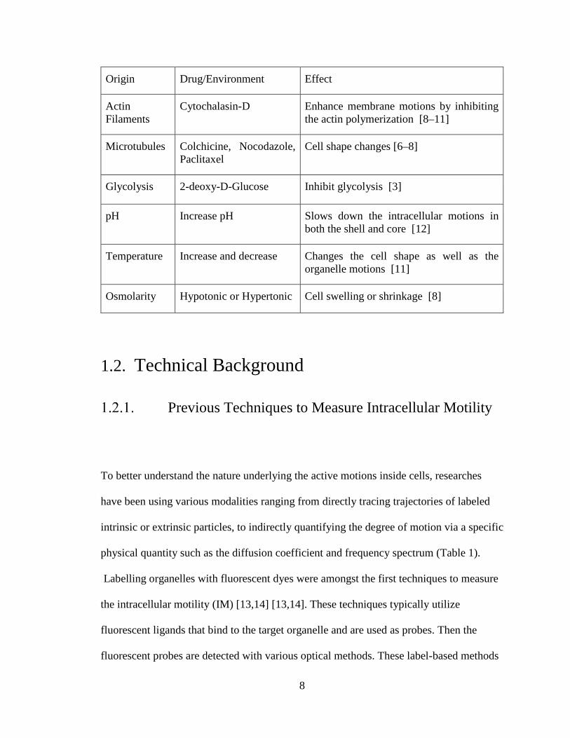
Effects of Environmental Change and Chemical

Treatment on Intracellular Motility

Studies on the effects of environmental changes and chemical treatment on intracellular

motility are tabulated below (Table 1) [3, 6–12] . The intracellular motility was

measured using various methods outlined in the next section. As for environmental

changes, the pH level, temperature, and osmolarity have been shown to lead a change in

the intracellular motility. Chemical treatment shown to result in a change in the

intracellular motility are generally those that either inhibit activity of the intracellular

components such as actin filaments and microtubules so that the structural change in

cytoplasm can occur. Structural change can give rise to movement of the organelles

formerly represented as bending motion, which can be detected as intracellular motility

change. Inhibiting glycolysis also influenced intracellular motility, supporting our

hypothesis that the observed intracellular motility can represent the metabolism-related

cellular viability.

Table 1 Effect of environmental change and chemical treatment on the cell

8

Origin Drug/Environment Effect

Actin Filaments

Cytochalasin-D Enhance membrane motions by inhibiting the actin polymerization [8–11]

Microtubules Colchicine, Nocodazole, Paclitaxel

Cell shape changes [6–8]

Glycolysis 2-deoxy-D-Glucose Inhibit glycolysis [3]

pH Increase pH Slows down the intracellular motions in both the shell and core [12]

Temperature Increase and decrease Changes the cell shape as well as the organelle motions [11]

Osmolarity Hypotonic or Hypertonic Cell swelling or shrinkage [8]

1.2. Technical Background

Previous Techniques to Measure Intracellular Motility

To better understand the nature underlying the active motions inside cells, researches

have been using various modalities ranging from directly tracing trajectories of labeled

intrinsic or extrinsic particles, to indirectly quantifying the degree of motion via a specific

physical quantity such as the diffusion coefficient and frequency spectrum (Table 1).

Labelling organelles with fluorescent dyes were amongst the first techniques to measure

the intracellular motility (IM) [13,14] [13,14]. These techniques typically utilize

fluorescent ligands that bind to the target organelle and are used as probes. Then the

fluorescent probes are detected with various optical methods. These label-based methods

9

have been advanced from directly tracing the particles to quantifying other useful

properties such as applied force. To directly measure the applied forces, endogenous

cytoskeletal microtubules are used as probes. Due to its local bending motion, the

microtubules’ amplitude is useful in determining the applied force.

However, these methods are invasive in nature, posing several problems such as

phototoxicity, photobleaching, eventually making a non-viable condition for the sample.

To overcome such limitation, methods which do not include dyes have been advanced to

enable label-free measurements of IM. By analyzing light scattered from cells, quantities

such as frequency fluctuations and mean square displacement have been suggested to

represent intracellular movements.

Table 2 Previous methods to measure intracellular motion

Quantified measurement Method

Label-based technique

Velocity Photon Correlation Spectroscopy of fluorescence-labeled organelles [14]

Velocity1 Time-lapse video image intensification microscopy [13]

Mean square displacement, Creep compliance

Fluorescence correlation spectroscopy of fluorescence-labeled injected extrinsic particles [15,16]

Diffusion coefficient fluorescence recovery after photo-bleaching of fluorescence-labeled injected extrinsic particles [17,18]

Diffusion coefficient Fluorescence-labeled injected extrinsic particles [19,20]

1 Direct tracing of particles for measurement

10

Diffusion coefficient Fluorescence correlation spectroscopy of fluorescence-labeled injected extrinsic particles [8]

Label-free technique

Mean square displacement Image Correlation spectroscopy [21]

Frequency fluctuations Holographic spectroscopy [12]

Force spectrum Optical Tweezer/FSM [22]

amplitude (motility) and time scale (autocorrelation decay time)

OCT [23,24]

Signal Contrast, Autocorrelation.

OCT [25]

Phase shifts (optical path length variations)

Phase contrast microscopy [26,27]

Mean square displacement Quantitative phase microscopy [28]

Intensity autocorrelation function

Photon Correlation Spectroscopy [29]

Previous Techniques to Measure Intracellular Diffusion

Coefficient

Table 3 lists the studies done in pursuit of measuring diffusion coefficients from the inside

of cells. The techniques can be categorized into three types; direct measurement,

measurements with transfect, and measurements with probe particles. Although

measurements with probe particles provide information of how diffusive the cytoplasm is,

and how it varies with drug treatment or environmental changes, they measure diffusion of

11

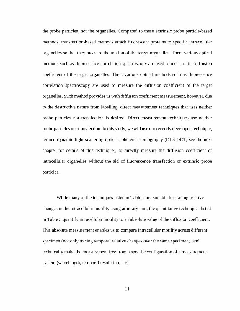
the probe particles, not the organelles. Compared to these extrinsic probe particle-based

methods, transfection-based methods attach fluorescent proteins to specific intracellular

organelles so that they measure the motion of the target organelles. Then, various optical

methods such as fluorescence correlation spectroscopy are used to measure the diffusion

coefficient of the target organelles. Then, various optical methods such as fluorescence

correlation spectroscopy are used to measure the diffusion coefficient of the target

organelles. Such method provides us with diffusion coefficient measurement, however, due

to the destructive nature from labelling, direct measurement techniques that uses neither

probe particles nor transfection is desired. Direct measurement techniques use neither

probe particles nor transfection. In this study, we will use our recently developed technique,

termed dynamic light scattering optical coherence tomography (DLS-OCT; see the next

chapter for details of this technique), to directly measure the diffusion coefficient of

intracellular organelles without the aid of fluorescence transfection or extrinsic probe

particles.

While many of the techniques listed in Table 2 are suitable for tracing relative

changes in the intracellular motility using arbitrary unit, the quantitative techniques listed

in Table 3 quantify intracellular motility to an absolute value of the diffusion coefficient.

This absolute measurement enables us to compare intracellular motility across different

specimen (not only tracing temporal relative changes over the same specimen), and

technically make the measurement free from a specific configuration of a measurement

system (wavelength, temporal resolution, etc).

12

Table 3 Previous methods to measure diffusion coefficient

Measured particles

Method Cell type Diffusion coefficient

[μm2/s]

Temperature [°C]

Organelles DLS-OCT [30,31]

living rodent cortex

0.1-10

Transfected organelles

k-space Image Correlation Spectroscopy [32]

MDCK GII cells cultured then, transfected with basolateral aquaporin-3 (AQP3-EGFP) and EGFP-AQP4 on collagen and E-cadherin:Fc surfaces : extracellular

0.014-0.044 37

Fluorescent correlation spectroscopy (FCS) [22]

Transfected HeLa cells with GFP (nano-sized proteins)

5-35 37

Extrinsic particles

Pulse-gradient spin–echo (s-PGSE) NMR technique [33]

Rat/Chicken erythrocytes Rat liver mitochondria In fluids (Not in a cell), intrinsic or extrinsic compounds used as probes

710-1810 25

Fluorescence recovery after photobleaching (FRAP)

Human neonatal foreskin diploid fibroblast cells grown in medium loaded with the indicated probe [34]

0.9-1 22

13

Swiss 3T3 cells cultured dextrans in cytoplasm as probes (with its size (2-40nm) being a factor for different diffusion coefficient) [17,18]

0.33~29 37

BG-9 human diploid fibroblast cells were cultured, and microinjected with probes [8]

25-47.2 37

Spot photobleaching

Fluorescence labeled DNA microinjected in HeLa cells cytoplasm [35]

3-50 23

Fluorescence Correlation Microscopy

Fluorescence labeled amino dextrans microinjected in cultured cells [36]

17-280 37

1.3. Objective and strategy

The objective of this study is to validate the DLS-OCT imaging of cellular viability by

characterizing responses of the measured intracellular motility to the environmental

conditions such as the temperature and pH, in animal retinal explant samples. As a

strategy, first step is to characterize our new OCT system and optimize scanning

sequences and processing procedures for DLS-OCT data, to match the dynamic range of

14

our DLS-OCT measurement with the typical range of intracellular motility. Both

numerical simulation and phantom experiments are performed for this optimization. Next

step is to establish methods required for animal retinal explant experiments, building

imaging chamber and the perfusion delivery and drainage system. Next, DLS-OCT data

from retinal tissue with different environmental conditions are performed and analyzed,

to test the technical hypothesis that DLS-OCT-measured intracellular motility of neurons

will significantly diminish. Similar approach is applied to tissue spheroids to test the

applicability of the method. Morphological observation is also performed with tissue

spheroid, to show the valuable potential of our system.

Previous studies with OCT to measure dynamics

Although OCT has been used in many studies especially for its ability to produce

tomographic information, measurement of dynamics of the sample has been limited.

Angiography and doppler has been widely used with OCT [37–42] to quantify blood flow

as flow index, morphological metric such as diameter and volume deformation [43] has

also been used as to show the dynamics. However, measurement of universally used

metrics such as diffusion coefficient or velocity have been lacking. Thus, providing

means to measure the universal quantity will aid in studies using OCT.

15

2.

DYNAMIC LIGHT SCATTERING

OPTICAL COHERENCE

TOMOGRAPHY

16

2.1. Introduction

Optical coherence tomography (OCT) is an emerging technology for label-free, three-

dimensional imaging of tissue structures with micrometer-scale resolution [44]. It has

been widely used for both clinical medicine including ophthalmology [45] and basic

research for neuroscience [46] and cancer biology [47]. Although its unparalleled

capability for structural imaging has been demonstrated to simultaneously achieve both

high spatial resolution and relatively large imaging depth, its capability for dynamic

imaging has been relatively less developed.

Dynamic light scattering (DLS) has been used for a long time to measure

diffusion or flow of particles. It analyzes fluctuations in light scattered by particles,

specifically its autocorrelation function. DLS has been mainly used for measurement of

the diffusion coefficient of gas molecules or micro-scale particles in a bulk sample, so it

has been challenging to apply DLS techniques for the measurement in biological

specimen which exhibit highly heterogeneous dynamics in the micrometer scale.

Since OCT uses coherence gating to collect light only scattered from a small volume for

the high-resolution structural imaging, integrating OCT with DLS could construct high-

resolution 3D maps of the diffusion coefficient and flow velocity, even in biological

specimen. The integration of two technologies has been demonstrated, termed DLS-OCT,

to provide us with a unique means to measure the diffusion coefficient and the flow

velocities at the same time, with the unprecedented resolution, and without the need of

extrinsic contrasts.

17

Previously, DLS-OCT imaging of the animal brain found high diffusion

coefficients in neurons; however, it is unclear whether the observed high diffusion

coefficients indeed represent cellular viability. Thus, there is a critical need to validate

the promising measurement capability in order to make the technology as a useful toolkit

and deploy it for a broad range of biomedical research.

2.2. Theoretical background

Optical Coherence Tomography

Michelson interferometer

The Michelson interferometer is one of the most commonly used interferometers for

scientific research, since it was first introduced in the late 19th century [48]. In a

Michelson interferometer, monochromatic light source travels through a beam splitter

and split into two arms. The split light beams travel to mirrors on each arm and reflect to

the beam splitter and then to a detector, where two light beams are interfered. Intensity of

the interference is measured with the detector z), and the interference signal is highly

sensitive to the relative positions of the mirrors so that the interferometer can detect a

slight movement of a mirror, generally down to 1/1,000 of the wavelength. The Laser

Interferometer Gravitational-Wave Observatory (LIGO) [49] is one of the latest

applications of this sensitive Michelson interferometer, which has successfully measured

a tiny signal of gravitational waves in 2016.

18

Figure 2 Schematics of interferometers. (a) Schematic of Michelson interferometer. (b) Schematic of time-domain optical coherence tomography.

19

Optical Coherence Tomography (OCT)

The principle of OCT is based on the Michelson interferometer. OCT analyzes the

interference between the light beam reflected or back-scattered from a sample and

another beam reflected from a mirror (called the reference mirror) as shown in Figure

2(b). When using a light source with low coherence (e.g., broadband light), the

interference only occurs when the photons scattered from the sample have the same

optical path length to those reflected from the reference mirror, and thus the detector can

measure the photons only scattered from the sample at a specific depth. By varying the

reference beam path length, OCT can explore different depths of the sample to obtain its

axial profile of reflectivity. Finally, by repeating this acquisition while scanning the probe

beam in the lateral directions, OCT can reconstruct a three-dimensional map of the

optical reflectivity of the sample. This is how the initial version of OCT works, called

time-domain OCT (TD-OCT). In summary, TD-OCT measures the axial reflectivity

profile, called A-scan profile, through scanning the optical path length of the sample

beam in time by moving the reference mirror.

In the last decade, OCT has been advanced to several different versions, including

spectral-domain OCT (SD-OCT), one of the most widely used versions. SD-OCT

replaces the detector with a spectrometer, to measure the interference pattern as a

function of the wavelength. Mathematically, the axial profile of the sample reflectivity

can be obtained using the inverse Fourier transform of this interference pattern. Thus,

SD-OCT does not need to move the reference mirror, dramatically increasing the imaging

20

speed and signal-to-noise ratio [50,51]. Furthermore, SD-OCT enables us to obtain the

optical reflectivity as the complex numbers (including the phase information of the

sample’s reflectivity), which was not possible with TD-OCT. In this thesis, we use a

latest high-speed SD-OCT system (Thorlabs Telesto III; 147,000 A-scan/s; 1,310-nm

center wavelength; 170-nm bandwidth; 3.5-um axial resolution).

Dynamic Light Scattering

Optical scattering theories

Depending on the size and shape of the scatterers, corresponding light scattering theories

are applied. For a spherical particle, Mie theory is applied. However, when the particle

size is much smaller than the wavelength of the incident beam, the Mie theory can be

approximated to Rayleigh scattering. In Rayleigh scattering, light scatters forward and

backwards in symmetry.

Photons are known to scatter most strongly by particles whose size is similar to

the light wavelength in the order of magnitude and whose refractive index mismatches

that of the surrounding medium. The refractive indices of common tissue components are

1.35-1.36 for extracellular fluid, 1.36-1.375 for cytoplasm, 1.38-1.41 for nuclei,

mitochondria and organelles. Generally, cell nuclei and mitochondria are strong scatterers

for visual and near-infrared light [52].

Fundamentals of dynamic light scattering analysis

21

When scatterers move, light scattered from them exhibits fluctuations. DLS is a set of

theories to describe how the time-varying light scattering results from dynamics of the

scatterers. In particular, it is well known that the autocorrelation function of the time-

varying electric field of scattered light shows an exponential decay when scatterers

exhibit Brownian motions, with the exponential decay constant being proportional to the

diffusion coefficient of the Brownian motion [53,54].

DLS has been used to measure the diffusion coefficient for various particles such

as proteins, polymers and nanoparticles [55], but mostly in bulky samples without high-

resolution 3D imaging capability. The previous methods were more like ensemble-

averaged point measurements.

Dynamic Light Scattering Optical Coherence Tomography

(DLS-OCT)

DLS model for the integration with OCT

With the assumption that static and moving particles are mixed in an OCT resolution

volume and that the moving particles can exhibit either translational or diffusive motion,

the 4D (space and time lag) field autocorrelation function of the 4D (space and time) SD-

OCT signal is given as [30]:

𝑔𝑔(𝒓𝒓, 𝜏𝜏) = ⟨𝑅𝑅∗(𝒓𝒓,𝑡𝑡)𝑅𝑅(𝒓𝒓,𝑡𝑡+𝜏𝜏)⟩𝑡𝑡⟨𝑅𝑅∗(𝒓𝒓,𝑡𝑡)𝑅𝑅(𝒓𝒓,𝑡𝑡)⟩𝑡𝑡

( 4 )

22

= 𝑀𝑀𝑆𝑆(𝒓𝒓) + 𝑀𝑀𝐹𝐹(𝒓𝒓)𝑒𝑒−ℎ𝑡𝑡2𝑣𝑣𝑡𝑡2(𝒓𝒓)𝜏𝜏2−ℎ2𝑣𝑣𝑧𝑧2(𝒓𝒓)𝜏𝜏2𝑒𝑒−𝑞𝑞2𝐷𝐷(𝒓𝒓)𝜏𝜏𝑒𝑒𝑖𝑖𝑞𝑞𝑣𝑣𝑧𝑧(𝒓𝒓)𝜏𝜏 + [1 −𝑀𝑀𝑆𝑆(𝒓𝒓)−𝑀𝑀𝐹𝐹(𝒓𝒓)]𝛿𝛿(𝜏𝜏)

Where R(r,t) is the reflectivity at given position r(x,y,z) and time t, and MS(r),

MF(r), vt(r), vz(r), and D(r) are the parameters of particle dynamics to be estimated for

each position. MS is the composition ratio of static particles, MF is that of

flowing/diffusing particles, vt is the transverse component of the flow velocity, vz is the

axial component, and D is the diffusion coefficient. The other parameters are defined in

the citation [30].

The general behavior of this autocorrelation function is illustrated in Figure 3(b).

For given voxel, the static term (MS) is the center of rotation, and MF is the initial

amplitude of rotation, which we assume do not vary during a short correlation time (in

the order of millisecond). The axial velocity-dependent phase term (𝑒𝑒𝑖𝑖𝑞𝑞𝑣𝑣𝑧𝑧(𝒓𝒓)𝜏𝜏) determines

the speed of rotation and the diffusion-oriented decay term (𝑒𝑒−𝑞𝑞2𝐷𝐷(𝒓𝒓)𝜏𝜏) determines decay

of the amplitude of rotation. However, the decay of the amplitude of rotation is not

simply an exponential decay in that it is also affected by the velocity-dependent term

(𝑒𝑒−ℎ𝑡𝑡2𝑣𝑣𝑡𝑡2(𝒓𝒓)𝜏𝜏2−ℎ2𝑣𝑣𝑧𝑧2(𝒓𝒓)𝜏𝜏2). By taking this term into account, we can estimate the transverse

component of the flow velocity as well as the axial component provided by the phase

term.

23

Figure 3 Conceptual illustration of the DLS-OCT theory. (a) Particles within the OCT resolution volume can be categorized into three groups: static, flowing or diffusing, and entering or exiting particles. For clarification, entering/exiting particles enter or exit out of the voxel during a single measurement time step, resulting in stochastic fluctuations of the OCT signal. (b) The general behavior of the field autocorrelation function in the complex plane predicted by our model. MS and MF are approximately proportional to the fractions of static and flowing/diffusing particles, respectively, weighted by their scattering cross-sections [30].

Previous results using DLS-OCT

Results from rodent brain imaging [31] showed that we can measure the cerebral blood

flow velocities. Also, in the data, it is found that neurons exhibit higher diffusion

coefficients than neighboring tissue. This data suggests the feasibility of label-free,

quantitative imaging of intracellular motility. Whether the relatively high diffusion

coefficients found from cells indeed represent cellular viability, however, needs

validation, which is one the major objectives of this thesis.

24

2.3. DLS-OCT simulation

Motivation for Simulation

We performed numerical simulations to meet two technical needs. First, we need to

optimize the scanning sequence parameters of the number of A-scans at each position (nt)

and the maximum time lag in the autocorrelation function (maxlag) toward accurate

measurement of the diffusion coefficients (D) over the range of intracellular motility

reported in the literature (Table 3). We chose five values of D in the range of 0.3-30

μm2/s, with even intervals in log scale.

Second, we need to determine the extent to which ranges of the particle dynamics-

related parameters our measurement of the diffusion coefficient will be robust, including

the number density of diffusing particles (Nf) and the velocity of flowing particles (v).

When particles exhibit a mixture of random walk and translational flow (e.g., flowing

Brownian particles), and when the velocity of the flow is too large compared to the

diffusive motion, the distinctive measurement of the diffusion coefficient against the

dominating flow velocity will not be sufficiently robust. Similarly, when the number

density of diffusing particles (Nf) in the imaging volume is too small (e.g., only 2

particles exhibit random walks while the other 98 particles do not move), the signal will

be very weak so that the measurement of the diffusion coefficient (of the small number of

the diffusing particles) will not be robust.

25

Procedures of Simulation

Process of numerical validation of our DLS-OCT measurement is summarized in Figure 4.

We generated two-dimensional (transverse and axial) position data of 100 particles for 100

time steps (∆t = 6.8 us) from the dynamic parameters. Position data were used to generate

SD-OCT signals, with which we obtained the first-order autocorrelation data. The

autocorrelation data generated for the combinations of parameters were fitted to determine

five independent coefficients (MS, MF, Vt, Vz and D), which minimizes the sum of squared

residuals (i.e. maximizing the coefficient of determination, R2). Finally, we compared

these estimated results with the true values calculated from the dynamic parameters,

position data and the SD-OCT signal.

Figure 4 Process of numerical simulation for validating the DLS-OCT theory. True values of the diffusion coefficient and velocity were determined by fitting the mean square displacement (MSD) of the numerical position data.

Simulation Results

26

Examples of the position data and corresponding OCT signals are displayed in Figure

5. They have a stochastic nature due to the random walk.

First, we confirmed that the behavior of g(τ) predicted by our theory (the Fig.

3(b)) is very close to that of the autocorrelation function of the numerically-generated

OCT signal, over a wide range of the dynamic parameters of NS, NF, NE, θ, v and D.

Several examples are shown in Figure 5.

Figure 5 Examples of the autocorrelation functions. Examples of the autocorrelation functions from the numerical position data and the fitting results are plotted. Here, D = 0.3 μm2/s.

The optimization was performed by iteratively selecting the set of measurement

parameters (nt , maxlag) toward minimization of error between the estimated and true

values of D, while exploring different ranges of the affecting dynamics parameters (Nf,

27

v). In detail, the criteria for the optimization was the root mean square (RMS) error of

MF⋅D, instead of D, because a small Mf can make the estimation result in an unreasonably

large D. We explored the values of nt = 100, 200 and 400 and maxlag = nt /2 and nt /4. As

a result, the measurement of MF⋅D was the most accurate with nt = 100 and maxlag =

nt/4, and it was robust over the ranges of Nf > 0.6 and v < 1 mm/s (Figure 6), leading to

the RMS error of 1.7%. This result implies that our analysis of the autocorrelation

function of the OCT signal, when acquired over nt= 100 and maxlag = nt/4, would

provide an accurate measurement of the diffusion coefficient (with less error than 2%)

over the range of 0.3-30 μm2/s, as long as more than 60% of the particles in the OCT

voxel exhibit a canonical random walk motions mixed with a smaller translational flow

than 1 mm/s.

Figure 6 Results of numerical DLS-OCT measurements. Results of numerical DLS-OCT measurements with the optimum measurement parameters (nt, τmax) and over the appropriate ranges of the dynamics parameters (Nf and v). The performance was tested for a total of 1,050 combinations (6 number densities, 5

28

diffusion coefficients, 5 velocities and 7 flow angles). ME= 1 - MS - MF. The points represent the mean and error from other combinations, while fixing the parameter of investigation.

Figure 7 The error in measurements of D and MF·D. (a) D (b) MfD over the whole range (c) Magnified view of the box in (b).

Discussion on Numerical Simulation

One of the major differences of our theory against previous ones is the g(τ) rotates in the

complex plane, not around the origin (which is assumed in most of previous theories), but

around a non-zero point (i.e., Ms in our theory). This was confirmed in the examples in

Figure 8, but we further investigated the decay of the magnitude of g. When the

magnitude of g(τ) relative to the origin point was plotted according to the previous

theories, the decay pattern was occasionally neither exponential (pure diffusion),

Gaussian (pure flow), nor a mixture of two (Figure 9). In contrast, when the magnitude is

plotted relative to the Ms point as predicted by our theory, the decay pattern was

relatively canonical (i.e., exhibited a mixture of exponential and Gaussian decays)

(Figure 9). This result supports that our novel approach enables accurate measurement of

29

the diffusion coefficient even when moving particles are mixed with static particles

within an OCT resolution volume. Other advantages include that we can estimate the

relative number density of moving particles (MF) and how the particle motions are close

to either canonical diffusive or translative motions (R2). When particles exhibit

oscillating motions for instance, it will result in a low R2 because our model did not

include such oscillating motions.

Figure 8 Examples of the autocorrelation functions with conventional theory. Examples of the autocorrelation functions of the numerical OCT data of the conventional theory. Here, v = 1 mm/s, and vz = 0 mm/s.

30

Figure 9 Examples of the autocorrelation functions with our new theory. Examples of the autocorrelation functions of the numerical OCT data follows our new theory than the conventional one. Here, v = 0.1 mm/s, and vz = 0 mm/s.

2.4. Experimental setup

Spectral-Domain Optical Coherence Tomography (SD-

OCT) System

A spectral-domain optical coherence tomography (SD-OCT) system (Thorlabs, Inc) is

used in this study. The SD-OCT system is optimized for DLS-OCT imaging. A large-

bandwidth near-infrared light source with center wavelength of 1310 nm, and wavelength

bandwidth of 170 nm is employed in the system for a large imaging depth and high

spatial resolution. The maximum imaging depth is 2.5 mm and the axial resolution is 3.46

31

um. The lateral resolution is determined by the objective lens in use. The 40x objective

lens (1-U2M587, LUMPLFLN 40XW, Olympus America, Inc) was used for cellular

imaging with its lateral resolution of 0.78 um. The scanning speed of the system is

147,000 A-scans/s.

DLS-OCT

Using the OCT system, we built LabVIEW software to control the system and acquire

data. Acquired data were post-processed using our lab software libraries in MATLAB.

The LabVIEW software includes a scanning sequence for DLS-OCT, and the software

libraries include a processing algorithm for DLS-OCT data. The published DLS-OCT

sequence and algorithm have been implemented with the previous OCT system with 47

kHz, where 100 A-scans were repeated, and the max time lag was 25 time points (~2 ms

range) [30]. In this study, we use the new OCT system with 147 kHz. Since the speed

(i.e., time lag sampling) and the number of A-scans (time lag range) affect the dynamic

range and accuracy of DLS measurement, we needed to optimize the scanning parameters

and processing algorithms for the new faster OCT system. For this reason, numerical

simulation was performed as in the previous section for the optimization and then

phantom measurements were conducted for calibration.

32

Simultaneous fluorescence imaging

To validate OCT imaging of individual cells (either by structural or dynamic contrast),

we built and integrated a component for simultaneous fluorescence imaging to the OCT

system. Figure 10 shows the schematic of the simultaneous imaging system. Blue light

with nominal wavelength of 490 nm from a mounted LED and a T-Cube LED Driver

(M490L4 and LEDD1B, Thorlabs) travels through the diffuser (ACL2520UDG6,

Aspheric Condenser Lens, Thorlabs) to the excitation filter (MF469-24, GFP Excitation

Filter, Thorlabs) and dichroic beamsplitter (69-899, Dichroic Longpass Filter, Edmund

Optics) where light direction is changed to the sample. The reflected light from the

sample travels through the beamsplitter and emission filter (FELH0500, Premium

Longpass Filter, Thorlabs) to the probe where the reflected lights are send to the

computer for real-time imaging and acquisition. The optics components were chosen so

that the OCT signal will neither crosstalk with the LED light nor be blocked.

33

Figure 10 Schematic of simultaneous imaging system.

Data Acquisition and Processing

SD-OCT system is used to acquire the OCT signal of the sample. SD-OCT system

parameters were (nt and maxlag) optimized in agreement to the result of the DLS-OCT

simulation. Data acquisition was performed using a labview file “Main.vi” in OCT

computer. Focusing was done with using “2D” and “3D” function in the file. Using “2D”

function, real-time B-scan views were shown, with which focal depth was set. With “3D”

34

function, real-time tomography was shown. After confirming the view of interest, data

was acquired using “ACQUIRE” function. In the next three sections, set of data

parameters used for each purpose is described. In the result sections, data gathered in a

different manner from the standard procedure will be explained as needed.

Reconstruction of a tomography

Three -dimensional SD-OCT signal data sized 512 pixels(W) X 512 pixels(H) X 1024

pixels(D) with transverse resolution of 0.5 um and axial resolution of 3.46 um was taken

using the 40x lens. A-scan and B-scan were both 1 and 4 identical volumes were taken

for volume averaging. The signal data was then reconstructed using

“Main_Reconstruct.m”. Data specific identification information was changed in the code.

For larger volume, three -dimensional SD-OCT signal data sized 512 pixels(W) X

512 pixels(H) X 1024 pixels(D) with transverse resolution of 20 um and axial resolution

of 3.46 um was taken using the LSM03 lens (Scan Lens, Thorlabs) . A-scan and B-scan

were both 1 and 4 identical volumes were taken for volume averaging. The signal data

was then reconstructed using “Main_Reconstruct.m”. Data specific identification

information was changed in the code.

Reconstruction of a diffusion coefficient data



35

using the 40x lens. A-scans were repeated at a fixed position for 128 times and was

moved to next scanning position to scan a 3D volume of the sample. B-scan was 1 and 2

identical volumes were taken for volume averaging. 4 mosaic volumes were taken in a

row using MX = 4, x center =0.048mm. The signal data was then reconstructed using

“Main_ReconstructDLS.m”. Data specific identification information was changed in the

code. The depth of the data to be reconstructed was shown in the code. After confirming

the depth of interest, the signal data is then reconstructed and fitted to determine the five

independent coefficients (MS, MF, Vt, Vz and D).

Reconstruction of a decorrelation data



using the 40x lens. B-scan was repeated 2 times over time interval of 10 ms and 20

ms. and 2 identical volumes were taken for volume averaging. The signal data was then

reconstructed using “Main_ReconstructAngio.m”. Data specific identification

information was changed in the code.

2.5. Results and discussions

Characterization of the System

Our DLS-OCT measurement algorithm includes the parameter of h and ht as in Eq.4,

which are functions of the spatial resolution [30]. Thus, it is important to accurately

36

measure the actual resolution of our system prior to DLS-OCT imaging of biological

specimen.

A 40X objective lens (water-immersed; 1-U2M587, LUMPLFLN 40XW,

Olympus America, Inc) is used with our SD-OCT system for cellular resolution. The

manufacturer specifications for the numerical aperture (NA) is 0.8, and working distance

is 3.3 mm. When used with our light source (center wavelength = 1.3 μm), the theoretical

lateral resolution is:

𝑟𝑟 = 0.61 𝜆𝜆1.3𝑁𝑁𝑁𝑁

= 0.76 (µ𝑚𝑚) ( 5 )

To determine the actual resolution with our OCT system, we measured the resolution with

a resolution target (1951 USAF Hi-Resolution Target, Edmund Optics). Figure 11(a)

shows the maximum intensity projection of the 3D image data (512 pixels X 512 pixels X

1024 pixels, width, depth, and height respectively, with transverse resolution of 0.5 um and

axial resolution of 3.46 um). Here, we applied Rayleigh criterion [56] to calculate the

lateral resolution. To determine the lateral resolution from the recorded data, intensity plots

of the line pairs in the targets were investigated. Selected area in Figure 11(a) was the

narrowest line pairs that was resolved according to the Rayleigh criterion. The lines had

width of 0.87 μm, which closely follow the theoretical resolution than the theoretical lateral

resolution.

37

𝐼𝐼0 = 𝐼𝐼 8𝜋𝜋2

( 6 )

Figure 11 Lateral resolution calculation using Rayleigh Criterion. (a) Maximum intensity projection of the 3D volume (1024 pixels X 512 pixels X 512 pixels) image from SD-OCT signal. (b) Magnified view of the area of interest marked in (a). (c) The intensity of the white line in (b).

Figure 12 shows the Rayleigh criterion and I/I0 for different line pair width. Line with

0.87 um as its width is the narrowest line to be resolved according to the criteria as

discussed above. Line with width of 0.78 um does not satisfy the criteria.

38

Figure 12 Normalized intensity plot of USAF target. Normalized intensity plot of USAF target per line width with Rayleigh criterion as a comparison (Line).

Phantom measurement of diffusion coefficient

We performed phantom (standard sample) experiments to validate that DLS-OCT can

accurately measure the diffusion coefficient, using previously optimized parameters from

the simulation following the standard procedure described in section 2.4.4.2.

Diffusion coefficient measurement from static sample

Diffuse reflectance standard (WS-1, Ocean Optics) was used as a static sample. Given

that true values of the parameters should be MS =1, MF, Vt, Vz, D =0, the data collected

from this sample was used to determine the kernel size for ensemble averaging of

autocorrelation function and whether to compensate for global phase shift. Median filter

39

and gaussian filter sizes were also determined using the data. The performance was tested

for a total of 24 combinations (2 kernel sizes for ensemble averaging, 2 options for global

phase shift, 2 window sizes for median filter and 3 window sizes for gaussian filter). The

optimal combination was determined such that it results in the minimum D. We found

that D was minimum as 0.054± 0.024 um2/s (R2=0.97) when the kernel size for ensemble

average was a 3 by 3 by 3 array with uniform values that sum up to 1, global phase shift

was not compensated, median filter size of 3 and gaussian filter size of 5 for the static

sample. The resulting en face plots of diffusion coefficient, velocity, and coefficient of

determination for the static sample with optimal conditions are shown in Figure 13. In

consequence, our DLS-OCT technique has the baseline noise of 0.054 um2/s in the

diffusion coefficient measurement.

Figure 13 Static sample measurement. Diffusion coefficient, velocity, and coefficient of determination for the static sample measurement with the optimal fitting condition.

40

Microspheres as standard samples

Microspheres were used to measure the diffusion coefficient using our methods. The

diffusion coefficient and diameters of the particle have an inversely linear relationship as

given by Stokes-Einstein equation. Thus, we used microspheres with different sizes to

validate the diffusion coefficient measurement. Standard procedure described in section

2.4.4.2 was used to collect and process the data. Monodisperse polystyrene microspheres

in 2.5% solids (w/v) aqueous suspension (Polysciences, Inc.) with diameters of 0.05 μm,

0.07um, 0.1 μm and 0.15um were used. We compared these estimated results with the

theoretical values of diffusion coefficient as given by Stokes-Einstein equation. Our OCT

system with the fitting algorithm have measuring range of 2.8um3/s to 8.1 um3/s, which

includes the diffusion coefficients of previously measured biological tissues (Table 3). As

shown in Fig. #, DLS-OCT-measured diffusion coefficients followed the general trend in

the theory. Note that microspheres have packed structure, which limited light penetration.

This prevented measuring the diffusion coefficient beyond our lower bound.

41

Figure 14 Phantom sample measurements of diffusion coefficients. Microspheres with diameter 0.05um, 0.07um, 0.1um and 0.15um were used. The circles with error bar indicate the measurements of the sample, the line indicates the theoretical diffusion coefficient.

Simultaneous OCT and fluorescence imaging

To confirm the correspondence between fluorescence imaging and OCT image,

fluorescent microspheres (17151-10, Fluoresbrite® YG Microspheres 0.20µm,

Polyscience, Inc) were used. The microspheres were suspended in Polydimethylsiloxane

(PDMS) to be made into a static fluorescent sample and were imaged using the 40x

objective lens. Fig. # shows the image reconstructed from OCT (a) and corresponding

42

image with fluorescence imaging. Red arrows indicate the corresponding figures in each

image. Note that more fluorescent lump appears in the fluorescence imaging due to the

characteristic difference of the imaging methods. The fluorescence imaging captures all

the features in the focal depth whereas the OCT captures a three-dimensional data and

shows each slice. Here in Figure 15 (a), maximum intensities from 5 neighboring depth

layers in focal depth (corresponding to 17.3 um) were projected to make a maximum

intensity projection. It can be inferred that within those 5 layers, the five distinctive

lumps were present.

Figure 15 Simultaneous imaging of fluorescent microbeads. Acquired image of fluorescent microbeads from OCT signal (a) and fluorescence imaging (b) using 40x lens. Red arrows indicate the corresponding figures in both images.

USAF target was also used to further confirm the correspondence between the

images. Here, LED was not used. Figure 16 shows the two images taken from OCT and

the camera with 40x lens. From these images, we determined the mapping function

43

between the OCT and fluorescence microscope. When OCT imaged the area of 32.5 um X

80 um around the center with 65 pixel X 160 pixel, the microscope image (60 pixel X 120

pixel) could be best overlapped to the OCT MIP image when transformed by a mapping

function of x’ = 0.94x-0.59 and y’ = -0.41y+0.88.

Figure 16 Images of 1951 USAF target. Images of 1951 USAF target from OCT signal (a) and OCT camera (b) using 40x lens. White dotted circles indicate the corresponding area.

44

3.

CELLULAR VIABILITY

MEASUREMENT OF

RETINAL NEURONAL CELLS

45

3.1. Introduction

Mouse retina has served an important role for studies of genetics and investigating

diseases and treatments [57,58] owing to its structure being layers of different types of

neurons being apparent a homogeneous within the layer. We chose the mouse retina as a

biological sample on which we validate the cellular viability measurement, because of the

unique laminar cell-type distribution and because our lab routinely dissects the retina

from mice.

As shown in the Table 1, changing environmental condition and drug

delivery can affect the motions inside a cell. The perturbation can be such that the

cell cannot survive or decrease in viability, which will either slow down or speed up

the motions, reflected on our diffusion coefficient measurement as a result. With our

hypothesis that DLS-OCT-measured intracellular motility of neurons will

significantly diminish when the cellular viability levels are out of the physiological

ranges, condition change was induced. From previous studies [10,12,59,60],

commonly used environmental changes were chosen to be change factor for our

experiment, the changes include temperature, ethanol treatment, osmolarity change,

and pH change. Lowering the temperature slows down molecular mobility [61], with

our hypothesis, lowering the temperature will decrease the diffusion coefficient

measurement. Ethanol, which can have cytotoxic effect, can cause complex

inhibition towards multiple cellular functions. However, it can also facilitate the

malfunction of the cells effectively. Osmolarity change influences cell

46

viability [62,63], however intracellular motility response to the osmotic stress is little

known. During hypotonic stress, cell swelling occurs, giving the molecules in

cytoplasm freedom to move, whereas during hypertonic stress, cell desiccation

occurs. The diffusion coefficient response to each condition was studied. Lowering

pH brings down viability [64,65], sometimes killing cells. This will also affect the

diffusion coefficient. Pilocarpine delivery was also performed, as a drug that targets

on affecting the cytoskeleton reorganization [66]. These modifications in active

cytoplasmic motion will have a significant impact on the diffusion coefficient

variance.

3.2. Experimental methods

Retinal dissection and handling

Mice were placed in a closed anesthesia chamber, and anesthesia is induced using 3-5%

isoflurane with mixture of 100% oxygen in air. Immediately after the initiation of

anesthesia, pharmaceutical grade Dexamethasone (0.2 mg/kg, IP for) is administered to

decrease inflammation, and buprenorphine (0.05-0.1 mg/kg IP) is administered to ensure

pain relief. The animal is examined to ensure that the level of anesthesia is sufficient to

prevent hindpaw reflexes, whisking behavior and corneal reflexes. Living whole retinas

or retinal slices were harvested directly from the euthanized animal and maintained in

vitro so that we can study neurons electrophysiologically or by functional imaging. The

surgical sites were clipped to remove fur and the site was cleaned using betadine

47

alternated with alcohol and repeated three times in total. The detailed method was:

Puncture the eye. Cut out the cornea. cut around the eye at the limbus, very close to the

limbus (retina is attached to the eye cup into 2 places: at the limbus and the optic disk), to

release the retina. After the cut around the limbus, place a forcep in the optic disk to fix

the eyecup, now gently with the other forceps (preferably blunt tip), go around the edges

to free the retina from the eyecup. Now the retina is fixed only at the optic disk, with the

forceps used to fix the optic disk, pressurize the area so that the optic nerve is damaged

and frees the retina or go from beneath the retina and hold the optic nerve and try to pluck

the retina gently. During surgery, the animal was monitored for anesthetic depth and

well-being by monitoring the body temperature, the respiration (character, depth,

frequency) and the pedal reflex. All the procedures were performed under the approval by

IACUC (1510000167).

The dissection is done in a dark room to prevent light exposure to the neurons,

then the sample is put on a filter (Millicell Cell Culture Insert, EMD Millipore Corp.),

sucked from the other side to be fixed at the surface. Then the sample and the filter are

placed in an imaging chamber covered entirely, so that during the delivery to the imaging

dark box, light exposure is minimized.

Fluorescence imaging preparation

For simultaneous OCT and fluorescence imaging, genetically encoded calcium indicator

(GCaMP) transgenic mice were used for green fluorescent protein (GFP)

excitation [67]. Wild-type mice were also used by staining the neuronal cells with

48

Calcium indicator (Oregon Green, Thermo Fischer Scientific). To prepare a wild-type

mouse retina for fluorescence imaging, the mouse was kept in dark for adaptation for an

hour during which AMES medium was prepared and bobbled. After the adaptation, eyes

were enucleated from the mouse and cornea, vitreous, and lens were removed. The

eyecup was to be left with sclera then the eyecup. The eyecup was incubated in papain

(Worthington Biochemical Corporation) and Ames solution for 20 minutes for removal

of the inner limiting layer while retinal neuronal cells are facing up. After 20 minutes in

papain solution, the supernatant was removed, and the eyecup was incubated in

ovomucoid for another 10 minutes to inhibit the papain enzyme destroying the neuronal

cells. After treating in ovomucoid, remove the supernatant and wash the eyecup using

AMES medium. The eyecup now can either be treated in calcium indicator before

dissection or be dissected and treated in calcium indicator for 30 minutes. The retinal

tissue is ready after washing the calcium indicator. During the process, 95% O2 and 5%

CO2 gas was supplied to the incubator while maintaining the temperature at 36.5°C.

Image acquisition

Images acquisition system

For the image acquisition of the mouse retina, a dark box is prepared (Figure 17). From

the dissection to the imaging, the retina was not exposed to light, because light exposure

can stimulate neurons, resulting in functional change in the sample [68,69]. The box with

size of 15” X 15” X 20” was assembled with construction rails, then covered with black

poster board and blackout fabrics on an Aluminum breadboard. SD-OCT system is

49

located inside the box with the fibers and cables connected to the computer accessed

through a slit in the bottom of the dark box. The slit is then covered with the blackout

fabric to prevent lights from penetrating. The frontal area of the box is covered with

extra-long blackout fabric for flexibility of the access to the interior of the box. Tubings

for supplying and draining the perfusion system are also accessed in the same manner.

Figure 17 Dark box setup for image acquisition. Retina imaging chamber is located below SD-OCT for image acquisition. SD-OCT system and the retina chamber are inside a dark box.

Retina imaging chamber and the filter holder were designed with Solidworks

(Dassault systemes) (Figure 18(a)) and printed with a 3D printer (B9Creator v1.2,

B9Creations. LLC) (Figure 18 (b)). The retina imaging chamber has two open walls on

each side so that the perfusion can be supplied from one end of the chamber and the

waste can be drained on the other end of the chamber without disturbing the imaging area

by minimizing the perturbation of the fluid. On the bottom of the chamber at the center,

50

there are three legs where the filter holder is placed. The three legs prevent the filter

holder from floating inside the chamber. The filter holder holds a filter, on which

dissected retina is placed.

Figure 18 Retina imaging chamber. (a) Assembled retina imaging chamber and filter holder design in Solidworks. (b) 3D-printed product of the model attached to the breadboard. The image shows the needles used for perfusion supply system.

Detailed perfusion supply and drainage system is shown in Figure 19. Ames

medium [70] (Sigma-Aldrich Corp.) in a borosilicate glass aspirator (Kimble) is bobbled

by O2 (5% CO2). Ames medium is prepared by dissolving one bottle of AMES medium,

1.9 g of NaHCO3, and 1.8 g of glucose to 1 L of distilled water. The medium goes

through a 3-way tubing connected to the bottom outlet, one of which can be used for drug

release, and the other goes through a syringe pump (AL-1000, WPI Inc.) for precise

controlling. The controlled flow then goes through a heater (SH-27B, Warner

instrument), controlled by a heater controller (TC-324C, Warner instrument) with a

sensor probe inside the chamber to maintain a desired temperature. Except for the set of

experiment with the temperature variance, we choose the temperature to be maintained at

51

33℃ [71,72], for the retina tissue to be active and healthy, which we will call normal

condition group. The temperature measured at the sensor often lower than the real

temperature in the tissue, because of the distance between the tube heater and the sensor

probe. The Ames medium travels inside the chamber to the other side of the chamber

where fluid outlet is located. A suction needle connected to a tubing with vacuum is

placed at a fixed position, so that the needle sucks any fluid that overflows the set level,

thus the amount of fluid in the chamber is kept at constant.

Figure 19 Schematic of the retina chamber. The perfusion medium bubbled with Oxygen with 5% CO2 then travels through the heater to be supplied to the retina chamber. Waste medium is sucked with vacuum on the other end of the chamber.

52

SD-OCT

As discussed in the section 2.4.4.2, standard procedures were taken for diffusion

coefficient measurement. After the fitting, 12 cells were selected manually from the

diffusion coefficient map, then cellular regions were chosen with the same three-

dimensional size of 5 pixels X 25 pixels X 25 pixels (17.3 um X 12.5 um X 12.5 um).

The average D value of each region of interest (ROI; representing each cell) was

computed, leading to 12 mean diffusion coefficient values. Then the 12 means were

averaged again to represent the diffusion coefficient (with an error bar; standard

deviation) of the data set. Note that these D values can be lower than the exact values in

the cytoplasm because the rectangular 3D ROI can involve the nucleus and extracellular

space in addition to the cytoplasm.

For decorrelation measurement, standard procedures were taken as discussed in

section 2.4.4.3. Although the decorrelation only provides a qualitative means to estimate

the intracellular motility, its relative changes in response to environmental manipulations

may give us another insight. We acquired the decorrelation data from the same samples

and in the same condition whenever we took the DLS-OCT data. Intensity of the tissues

can vary greatly which can affect decorrelation. Generally, higher intensity induces

higher decorrelation. Thus, we invite the concept of relative decorrelation, to normalize

the variance among the measurements. Here, relative decorrelation of a voxel is

decorrelation value divided by intensity value of a voxel. In most cases, average of the

intensity, decorrelation, and the relative decorrelation of the area of focus was calculated

from MIP and plotted in the figure. The area of focus had a size of 256 pixels X 256

53

pixels (128um X 128 um), chosen to minimize the intensity variance within the area.

Note that for experiments where osmolarity was changed, 12 cells were selected

manually, then cellular voxel data was generated with the size of 5 pixels X 25 pixels X

25 pixels (17.3 um X 12.5 um X 12.5 um). The average values of each cell were

computed to generate 12 average intensity, decorrelation, and relative decorrelation

values. Then the 12 averages were averaged again to represent each metrics.

Drug induce and temperature change

Temperature, osmolarity changes can be done simply by changing the level of the

components in our perfusion system. The temperature was varied by changing the heater

settings. To establish the osmotic pressure between the cell and the surrounding fluid was

controlled by changing the concentration of Sodium hydroxide in the Ames medium. PH

change was induced by undersupplying 5% CO2 and 95% O2 gas or adding hydrogen

chloride. Ethanol treatment (2.2 M) was also induced for its cytotoxic effect. Pilocarpine

was used to induce change in cytoskeleton.

54


Fluorescence imaging

Fluorescence imaging using GCaMP mice were performed to confirm the detection of the

cells in the metrics used. Figure 20(a-b) shows the fluorescence imaging result and the

decorrelation map to the corresponding area comparison. The red arrows in Figure 20(a)

have pattern that is also found in Figure 20(b). Part of the cells seen in the fluorescence

imaging is absent in the decorrelation map due to the difference of the imaging

techniques. Fluorescence imaging does not have the ability to penetrate the cells and

show the images as slices, thus the depth at which individual cells are present in the

image vary within the focal depth. On the other hand, with the tomographic map obtained

from SD-OCT shows the cells at certain depth. In addition, the use of 40x objective

causes confocal effect, which can distort the position of the cells. The diffusion

coefficient map was compared with the fluorescence imaging in the same manner (Figure

20 (c-d)). Fluorescence imaging identified the existence of cells within our field of view,

qualitatively in terms of sizes as well [73–77].

55

Figure 20 Comparison of cell images in fluorescence imaging and SD-OCT imaging. (a) Fluorescence imaging of the neurons. (b) Decorrelation map obtained using SD-OCT of the same areas as (a). (c) Fluorescence imaging of the neurons. (d) Diffusion coefficient map obtained using SD-OCT of the same areas as (c). The red arrows demonstrate the corresponding cell figures in both imaging methods.

Diffusion coefficient

Diffusion coefficient in cytoplasm was measured higher than that of the nucleus, due to the

higher movement in the cytoplasm whereas there is in the nucleus (Figure 21 (a)). Although

there are movements in the nucleus as well as between the nucleus and the cytoplasm such

as RNA transport [78], diffusion aroused from those movements were not captured

possibly due to its small size. The results in the normal-condition group varied across the

different samples from 0.2 um3/s to 30 um3/s. This large variance can arise from the

difference in the viability between the dissected samples [79,80]. During the dissection,

damages can be done physically to the neural cells and its functions. Therefore, rather than

comparing averages between the groups, we analyzed the relative changes within the same

sample, induced by environmental manipulation or chemical treatment, as detailed in the

previous section.

56

Maximum intensity projections in xy and yz planes Figure 21(b) and maximum

diffusion coefficient projections in xy and yz planes are shown in Figure 21(c), with the

window size of 17 pixels (8.5um) in x and y-axis and 7 pixels in z axis (24.22um).

Figure 21 Baseline measurement of diffusion coefficient. (a) Baseline measurement of diffusion coefficient in the normal-condition group. (b) Maximum intensity projections in xy, yz, and xz planes. (c) Maximum diffusion coefficient projections in xy, yz, and xz planes. Scale bar: 5um

Temperature

Diffusion coefficient change in reaction to the temperature change from viable body

temperature around 36.5°C to 13°C is shown in Figure 22. The diffusion coefficient was

measured after 30 minutes of exposure to the changed temperature. Viability of the cells

and tissues worsens as temperature deviates from body temperature. Diffusion coefficient

57

also decreased as temperature decreased. Diffusion coefficient is related to the

intracellular motility which originate from active movements in the cytoplasm. It is

reported that routine metabolic rate decreases as temperature changes [81]. Intracellular

motility retard from the temperature drop was observed as diffusion coefficient drop

resultantly.

Figure 22 Diffusion coefficient of the retinal neural cells to different temperatures. (a) Diffusion coefficient map of the retinal neural cells at normal condition. (b) Diffusion coefficient map of the retinal neural cells at 15°C. Scale bar: 10um (c) Red bar indicates the diffusion coefficient of the retinal neural cells at 31°C. Blue bar indicates the diffusion coefficient at 15°C.

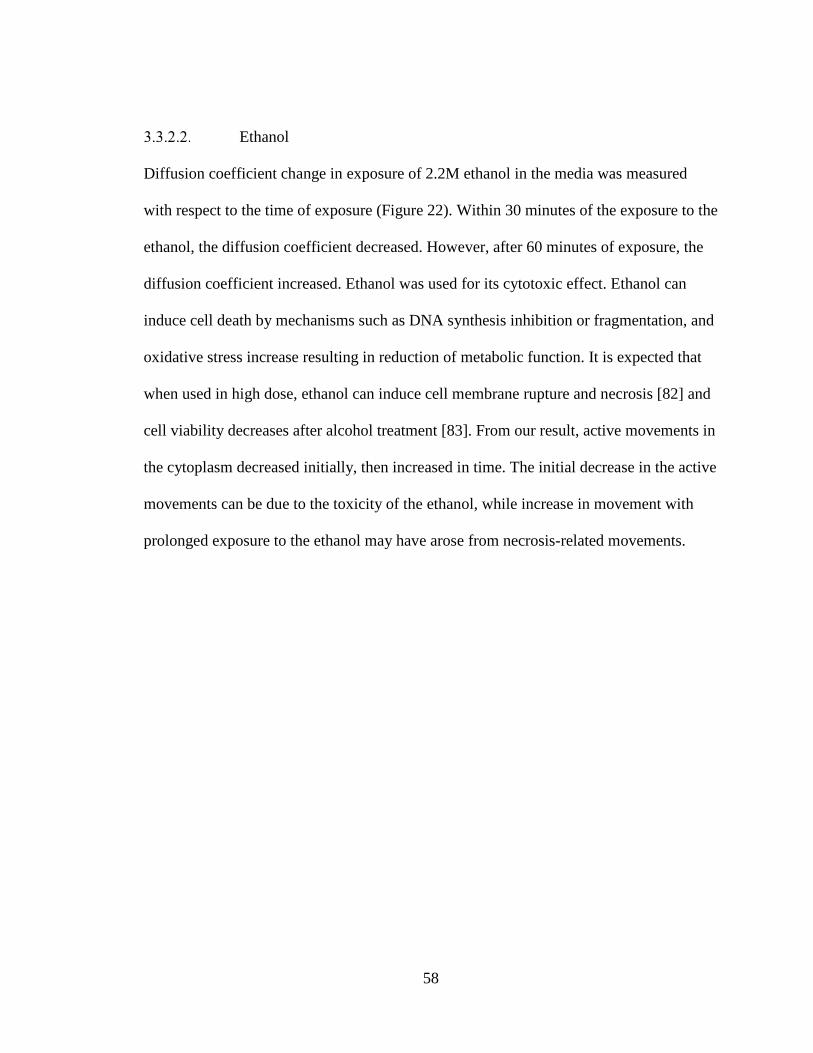
58

Ethanol

Diffusion coefficient change in exposure of 2.2M ethanol in the media was measured

with respect to the time of exposure (Figure 22). Within 30 minutes of the exposure to the

ethanol, the diffusion coefficient decreased. However, after 60 minutes of exposure, the

diffusion coefficient increased. Ethanol was used for its cytotoxic effect. Ethanol can

induce cell death by mechanisms such as DNA synthesis inhibition or fragmentation, and

oxidative stress increase resulting in reduction of metabolic function. It is expected that

when used in high dose, ethanol can induce cell membrane rupture and necrosis [82] and

cell viability decreases after alcohol treatment [83]. From our result, active movements in

the cytoplasm decreased initially, then increased in time. The initial decrease in the active

movements can be due to the toxicity of the ethanol, while increase in movement with

prolonged exposure to the ethanol may have arose from necrosis-related movements.

59

Figure 23 Diffusion coefficient of the retinal neural cells to exposure of 2.2M of ethanol in the media. (a) Diffusion coefficient map of the retinal neural cells at normal condition. (b) Diffusion coefficient map of the retinal neural cells 30 minutes after alcohol treatment. Scale bar: 10um (c) Red bar indicates the diffusion coefficient of the retinal neural cells at 31°C. Blue bar indicates the diffusion coefficient when the tissue was exposed 30 minutes and 60 minutes, respectively.

Osmolarity

AMES media used for in this study has isotonic osmolarity of 329 mOsm designed to

provide a physiological osmolarity. The change in osmolarity can induce either cell

swelling under hypotonic condition or cell shrinkage under hypertonic condition, both of

which can give rise to the change in diffusion coefficient.

60

The temperature was maintained at normal condition at 0 minute. The temperature

and CO2 level were maintained all throughout the experiment, except when pH change

was induced. Ames media with higher or lower osmolarity was supplied to reach either

hypertonic or hypotonic condition.

Exposure to the hypotonic stress (200 Osm) lead to increase in diffusion

coefficient in time (Figure 24(c)). The diffusion coefficient increase in hypotonic

condition may have relation to the active movements of the organelles because the

reconstructing of the membranes to prevent the rupture of the membranes draws extra

membranes and intracellular reserves to the surface [84,85].

Decrease in diffusion coefficient was observed in exposure to the hypertonic

stress (500 Osm) in time (Figure 25(c)). Viability decline due to osmotic stress has been

studied [86,87], which may be source of the diffusion coefficient decrease seen here.

61

Figure 24 Diffusion coefficient of the retinal neural cells to exposure of hypotonic condition. (a) Diffusion coefficient map of the retinal neural cells before exposure to the hypotonic media. (b) Diffusion coefficient map of the retinal neural cells 65 minutes after exposure to the hypotonic media. Scale bar: 10um (c) Diffusion coefficient of the retinal neural cells with errorbar to the duration of exposure of hypotonic condition of 200 Osm at 31°C. The retinal tissue was exposed to the hypotonic condition at 0 minutes and the diffusion coefficient was measured at 15 minutes, and 65 minutes, respectively.

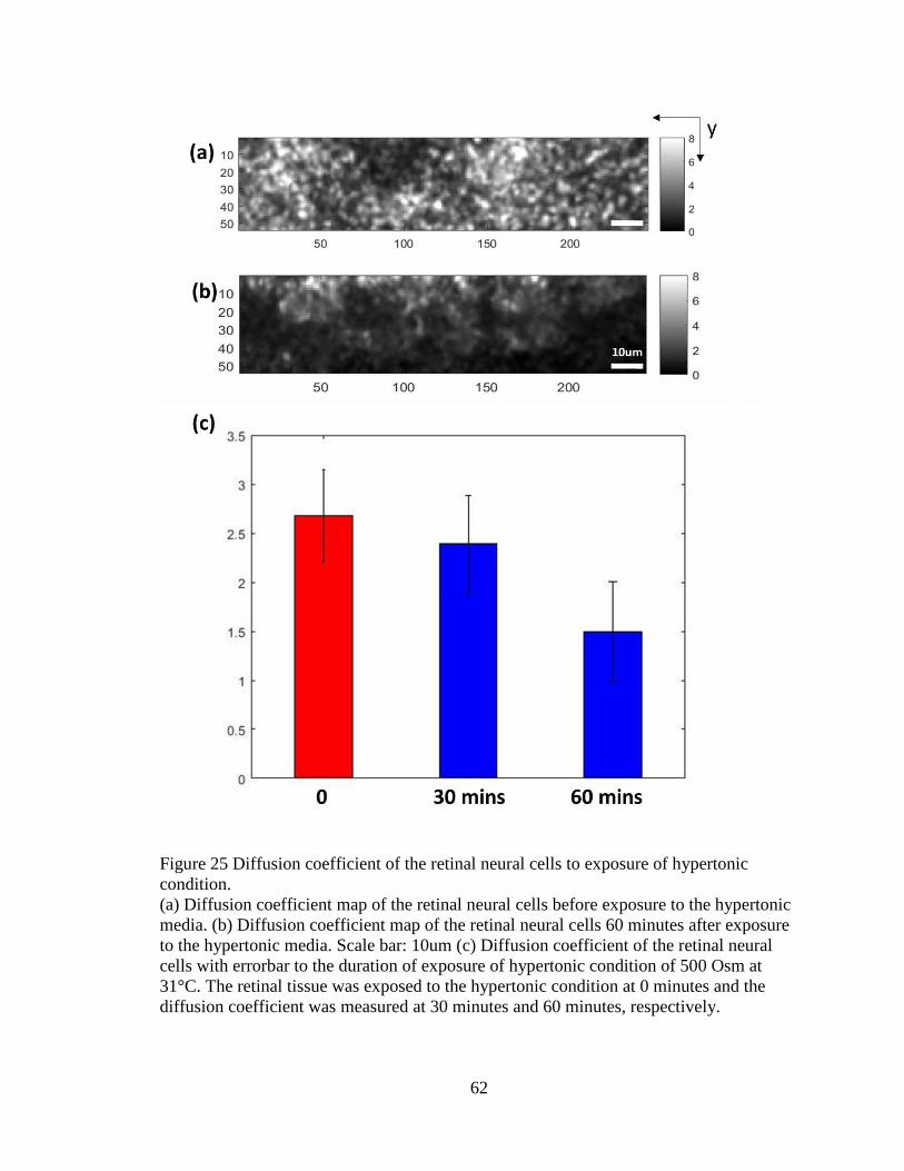
62

Figure 25 Diffusion coefficient of the retinal neural cells to exposure of hypertonic condition. (a) Diffusion coefficient map of the retinal neural cells before exposure to the hypertonic media. (b) Diffusion coefficient map of the retinal neural cells 60 minutes after exposure to the hypertonic media. Scale bar: 10um (c) Diffusion coefficient of the retinal neural cells with errorbar to the duration of exposure of hypertonic condition of 500 Osm at 31°C. The retinal tissue was exposed to the hypertonic condition at 0 minutes and the diffusion coefficient was measured at 30 minutes and 60 minutes, respectively.

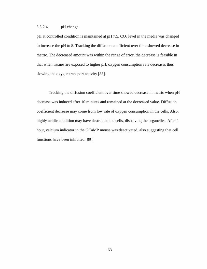
63

pH change

pH at controlled condition is maintained at pH 7.5. CO2 level in the media was changed

to increase the pH to 8. Tracking the diffusion coefficient over time showed decrease in

metric. The decreased amount was within the range of error, the decrease is feasible in

that when tissues are exposed to higher pH, oxygen consumption rate decreases thus

slowing the oxygen transport activity [88].

Tracking the diffusion coefficient over time showed decrease in metric when pH

decrease was induced after 10 minutes and remained at the decreased value. Diffusion

coefficient decrease may come from low rate of oxygen consumption in the cells. Also,

highly acidic condition may have destructed the cells, dissolving the organelles. After 1

hour, calcium indicator in the GCaMP mouse was deactivated, also suggesting that cell

functions have been inhibited [89].

64

Figure 26 Diffusion coefficient of the retinal neural cells to exposure of pH 8. (a) Diffusion coefficient map of the retinal neural cells before exposure to the higher pH. (b) Diffusion coefficient map of the retinal neural cells 60 minutes after exposure to the higher pH. Scale bar: 10um (c) Diffusion coefficient of the retinal neural cells with errorbar to the duration of exposure of increased pH of 8 at 31°C. The retinal tissue was exposed to the higher pH at 0 minutes and the diffusion coefficient was measured at 30 minutes and 60 minutes, respectively.

65

Figure 27 Diffusion coefficient of the retinal neural cells to exposure of pH 3.5. (a) Diffusion coefficient map of the retinal neural cells before exposure to the lower pH. (b) Diffusion coefficient map of the retinal neural cells 60 minutes after exposure to the lower pH. (c) Diffusion coefficient map of the retinal neural cells 60 minutes after exposure to the lower pH with different color limits to reveal the cell shapes. Scale bar: 10um. (d)Diffusion coefficient of the retinal neural cells with errorbar to the duration of exposure of decreased pH of 3.5 at 31°C. The retinal tissue was exposed to the lower pH at 0 minutes and the diffusion coefficient was measured at 30 minutes and 60 minutes, respectively.

66

Pilocarpine

Pilocarpine is known to induced epilepsy, and its association with actin cytoskeleton

reorganization has been reported [66]. The actin cytoskeleton reorganization can give rise

to a change in the intracellular motility. Diffusion coefficient change after 30 minutes of

exposure to the 10% pilocarpine in the media was measured and compared to the viable

condition (Figure 28). The diffusion coefficient increased in response to the pilocarpine

exposure, which can arise from the known active movements from actin cytoskeleton.

67

Figure 28 Comparison of diffusion coefficient of the retinal neural cells to the pilocarpine. (a) Diffusion coefficient map of the retinal neural cells at normal condition. (b) Diffusion coefficient map of the retinal neural cells 30 minutes after exposure to the pilocarpine. (c) Red bar indicates the diffusion coefficient of the retinal neural cells at 31°C. Blue bar indicates the diffusion coefficient when tissue is treated with pilocarpine for 30 minutes.

68

Decorrelation

This section presents the result from the decorrelation imaging. Figure 29 shows the

intensity, decorrelation, and relative decorrelation maps of 5 neighboring axial layers are

shown by averaging the layers, and cellular mappings of each metrics.

69

Figure 29 Intensity, decorrelation, and relative decorrelation maps. Intensity (a), decorrelation (b), and relative decorrelation (c) maps of 5 neighboring axial layers are shown by averaging the layers. Scale bar: 10 um. Cellular maps of Intensity (c), decorrelation (d), and relative decorrelation (e) are shown in xy, yz, and xz planes. Scale bar: 5 um.

70

Temperature

Figure 30 shows the intensity, decorrelation, and relative decorrelation response to the

temperature change. The relative decorrelations of the lower temperature were lower in

all cases and time steps. It can be inferred that there were more signal change and/or

movements in the tissue at viable condition of 33°C. More decorrelation is gained over

longer b-scan rate as shown in the figure. However, between 17 ms and 37 ms, there was

little change, thus time steps of 10 ms and 20 ms will be used.

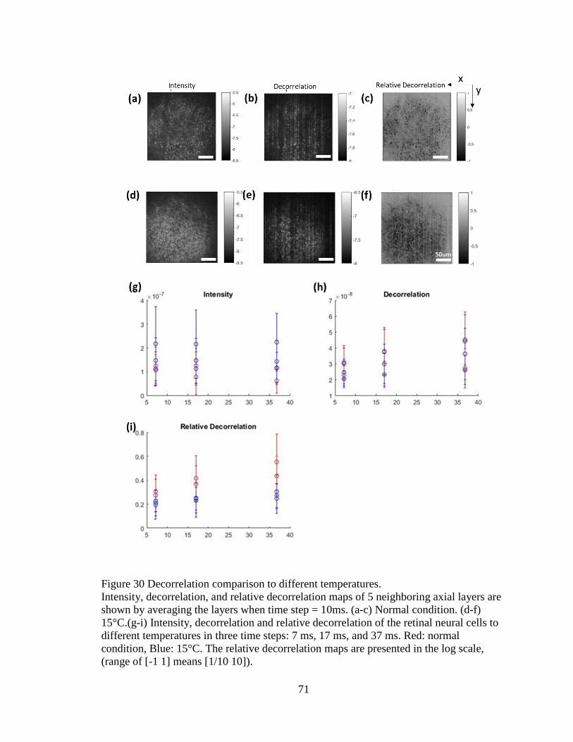
71

Figure 30 Decorrelation comparison to different temperatures. Intensity, decorrelation, and relative decorrelation maps of 5 neighboring axial layers are shown by averaging the layers when time step = 10ms. (a-c) Normal condition. (d-f) 15°C.(g-i) Intensity, decorrelation and relative decorrelation of the retinal neural cells to different temperatures in three time steps: 7 ms, 17 ms, and 37 ms. Red: normal condition, Blue: 15°C. The relative decorrelation maps are presented in the log scale, (range of [-1 1] means [1/10 10]).

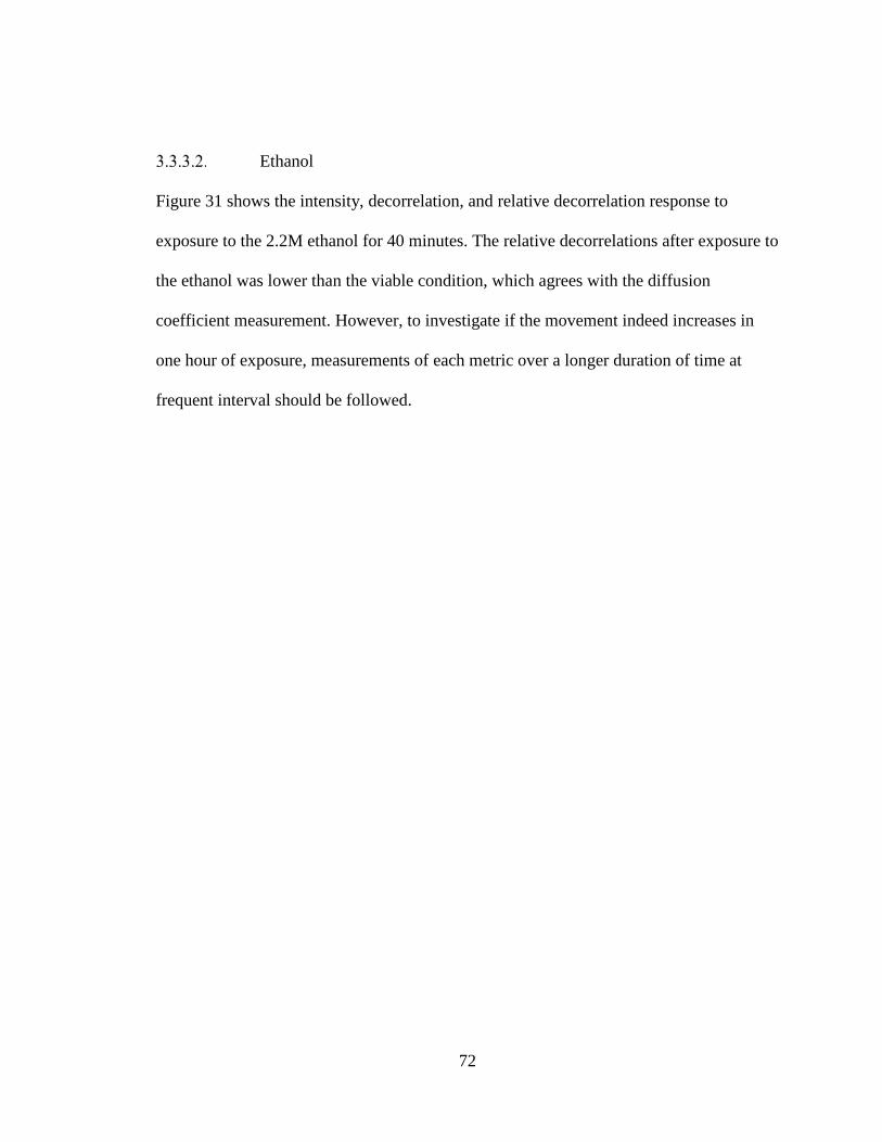
72

Ethanol

Figure 31 shows the intensity, decorrelation, and relative decorrelation response to

exposure to the 2.2M ethanol for 40 minutes. The relative decorrelations after exposure to

the ethanol was lower than the viable condition, which agrees with the diffusion

coefficient measurement. However, to investigate if the movement indeed increases in

one hour of exposure, measurements of each metric over a longer duration of time at

frequent interval should be followed.

73

Figure 31 Intensity, decorrelation, and relative decorrelation maps of 5 neighboring axial layers are shown by averaging the layers when time step = 10ms. (a-c) Normal condition. (d-f) after treating with 2.2M alcohol for 30 minutes. (g-i) Intensity, decorrelation and relative decorrelation of the retinal neural cells to different temperatures in two time steps: 10 ms and 20 ms. Red: normal condition, Orange: after treatment. The relative decorrelation maps are presented in the log scale, (range of [-1 1] means [1/10 10]).

74

Osmolarity

Figure 32 shows average of 12 selected cells from relative decorrelation data of each

data set. Relative decorrelation of the tissues’ response to the hypotonic stress over time

is plotted in Figure 32 Relative decorrelation increased over the duration of the hypotonic

condition, which agrees with the diffusion coefficient measurement.

75

Figure 32 Intensity, decorrelation, and relative decorrelation maps of 5 neighboring axial layers are shown by averaging the layers when time step = 10ms. (a-c) Normal condition. (d-f) after being in hypotonic condition for 65 minutes. (g-i) Intensity, decorrelation and relative decorrelation of the retinal neural cells to different temperatures in two time steps: 10 ms and 20 ms over exposure time. Red: normal condition, blue: hypotonic. Here, x-axis represents the exposure time to the hypotonic condition. The relative decorrelation maps are presented in the log scale, (range of [-1 1] means [1/10 10]).

76

pH

Figure 33 shows relative decorrelation data of each data set. Relative decorrelation of the

tissues’ response to the lower pH over time is plotted in Figure 33. Relative decorrelation

decreased after 10 minutes from the exposure and stayed in the lower decorrelation

throughout one hour. This result agrees with the diffusion coefficient measurement as a

response to the extreme acidic condition.

77

Figure 33 Intensity, decorrelation, and relative decorrelation maps of 5 neighboring axial layers are shown by averaging the layers when time step = 10ms. (a-c) Normal condition. (d-f) after exposure to low pH (pH 3.5) condition at 10 minutes. (g-i) Intensity, decorrelation and relative decorrelation of the retinal neural cells to different temperatures in two time steps: 10 ms and 20 ms. Red: normal condition, blue: after exposure to low pH condition at 0, 10, 20, 30, 40, 50, and 60 minutes, respectively. Here, x-axis represents the exposure time to the hypotonic condition. The relative decorrelation maps are presented in the log scale, (range of [-1 1] means [1/10 10]).

78

Pilocarpine

Treatment of 10 % Pilocarpine in the media brought increase in the relative decorrelation.

Under the same treatment, increase in diffusion coefficient was also observed. It can be

inferred that the actin cytoskeleton reorganization brings the signal change, which can

arise from more movement or optical property change in the cells.

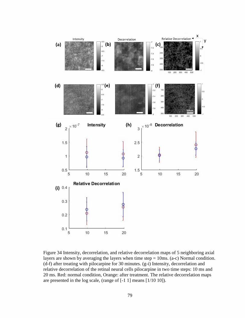
79

Figure 34 Intensity, decorrelation, and relative decorrelation maps of 5 neighboring axial layers are shown by averaging the layers when time step = 10ms. (a-c) Normal condition. (d-f) after treating with pilocarpine for 30 minutes. (g-i) Intensity, decorrelation and relative decorrelation of the retinal neural cells pilocarpine in two time steps: 10 ms and 20 ms. Red: normal condition, Orange: after treatment. The relative decorrelation maps are presented in the log scale, (range of [-1 1] means [1/10 10]).

80

3.4. Conclusions

Diffusion coefficient measurement and mapping was performed using ex vivo retina tissue.

Patterns observed in the D map were consistent with what we expect from the cellular

structure. And simultaneous imaging confirmed that the patterns truly represent

intracellular motility. We were also able to image intracellular motility even through

scattering tissues. When viability is manipulated using the conditions with well-known

effects, IM exhibited consistent changes with the known effect, except the long-term effect

of ethanol. However, the diffusion coefficient measurement at viable condition as a

baseline varied across the tissues, which may have arisen from difference in initial cellular

viability of the tissues. Studying the variance of the viability between samples will

strengthen the effectiveness of the diffusion coefficient measurement. The additional

metric relative decorrelation measurements also changed with changed conditions of the

tissue. Further studying into the matter will aid in understanding the change in cytoplasm

as signal intensity change or active movements inside.

81

4.

CELLULAR VIABILITY

MEASUREMENT OF TISSUE

SPHEROIDS

82

4.1. Introduction

Three-dimensional tissue spheroids are widely used to investigate the living organisms

owing to its benefit of simplifying the system. Measuring the viability of these tissue

spheroids has been in center of attention for many researches [90–93]. From chemical

assays to histology, many techniques have been applied. However, status of art still

requires destructive process to the tissues. Here we test the versatility of DLS-OCT by

investigating its capability in tissue spheroid viability imaging. In addition to the

diffusion coefficient, we test other metrics such as decorrelation and surface area to

volume ratio to gain knowledge of the relationships between viability and spheroid

structure.

Three -dimensional tissue spheroids are extremely useful tool to understand

behavior of organs or tumoroids, thus have been used in numerous studies in cancer

research, drug discovery. Tissue spheroids provide an environment well controlled for

research, compared to the in vivo samples in a host environment. It is also beneficial in

that the testing subject have flexibility in terms of testing procedures or availability

compared to living subjects. Especially when it comes to understanding tumoroids, the

similarity of the three-dimensional tissue spheroids to the tumor cells in vivo, such as the

presence of stroma and extracellular matrix (ECM) lead to the popularity of the tissue

spheroids.

83

Different cell types have different characteristics when they are seeded to form a

spheroid [94–96]. Unlike monolayer tissues which have non-distinctive forms, the shapes

of three-dimensional spheroid can range from round, mass, grape-like to stellate structure

groups [95]. While the shape of microwells in which the cells are seeded can affect the

structure of the tissue the seeded cells form, the seeding number also can affect the formed

shape. Final shape can also change as the day in vitro (DIV) increases, due to gravity,

necrotic core, surface tension, cytoskeleton movement, and debris because of the dead cells.

Cell shape difference as well as its growth and the physiological change including ECM

can result in optical property variance [97]. To study on how different cell types and shapes

are observed under our imaging technique and further image the viability difference, we

use two different types of cells.

Fibroblast

Fibroblast is known to take part in wound healing mechanism and it is one of stromal

cells which synthesizes the ECM and collagen. Being a key component in tumor

development with its relation to the tumor cell metastasis [98–101], proliferation [102]

and maintaining its shape, fibroblast has been a popular subject of study. In this study,

Fibroblast spheroids with seeding number of 1,000 cells/spheroid, 4,000 cells/spheroid,

and, 6,000 cells/spheroid were used (Morgan Lab). DIV 1 and DIV 14 samples were

studied. Fibroblast spheroid samples forms a mass-shaped spheroid with the current

seeding density.

84

HEP G2

Hep G2 is a cell line derived from a human liver carcinoma, which is known to exhibit

various morphological and functional in vitro, thus used for metabolic studies such as

lipoprotein mechanism, cholesterol synthesis and transport, and bile acids

synthesis [103]. In this study, Hep G2 cell spheroids with seeding number of 2,000

cells/spheroid, 4,000 cells/spheroid, and 8,000 cells/spheroid were used (Morgan Lab).

All the samples were DIV 1. Hep G2 spheroid samples forms a mass-shaped spheroid

with the current seeding density, however the shape at DIV 1 diverges from shape of

fibroblast which also forms a mass in that HEP G2 spheroids develop craters in the

center. The crater size differs across different seeding density.

4.2. Experimental methods

Microscopic imaging

Diffusion coefficient and decorrelation measurement methods are consistent with sections

3.3.2 and 3.3.3.

Macroscopic imaging

85

For macroscopic imaging, three -dimensional SD-OCT signal data sized 512 pixels(W) X

512 pixels(H) X 1024 pixels(D) with transverse resolution of 20 um and axial resolution

of 3.46 um were taken using LSM03 lens (Thorlabs). The signal data is then

reconstructed to generate macroscopic three-dimensional data that captures all the wells

in a 5 X 7 microwell (Mircotissues) each sized 800 um in diameter and in height which

holds a volume of 75 ul.

Surface area, volume, and dimensions measurement

A graphical user interface is written in matlab to easily gather the measurements. Once

raw data is reconstructed to obtain three-dimensional intensity data (see section 2.4.4.1),

the intensity array is loaded and shown as maximum intensity plots in all directions in the

Figure 35.

86

Figure 35 Maximum intensity projections in yz (a), xz (b), and x- and y axis (c) of a microwell with tissue spheroid inside. The tissue spheroids shown are HEP G2 spheroids with seeding number of 8,000 at DIV 1. Scale bar : 500um

The data is then cut in axial direction to obtain the three-dimensional array with

tissues inside (Figure 36(a)). Next, the data is cut in transverse direction to disregard any

unnecessary voxels (Figure 36 (b)‚ the maximum intensity plots of the resulting array are

87

shown in the Figure 36 (c-e) to ensure the user that the tissues are not cut in any

direction.

Figure 36 Maximum intensity projections in yz (a) and xy planes (b). The vertical and horizontal line in shows the user where they have chosen to cut eh arrays. Maximum intensity projections in yz (c), xz (d), and xy planes (e) of cropped array. The tissue spheroids shown are HEP G2 spheroids with seeding number of 8,000 at DIV 1. Scale bar: 500 um

With the updated intensity array, a threshold value is selected to make a binary

array of the tissues. Figure 37 (a-b) show the maximum intensity plot of the binary array

when higher threshold is applied. Although unnecessary voxels presenting defects or

debris are disregarded, tissues are also not fully included. When lower threshold is

applied (Figure 37 (c-d), the tissues are enclosed, but many voxels of the agarose

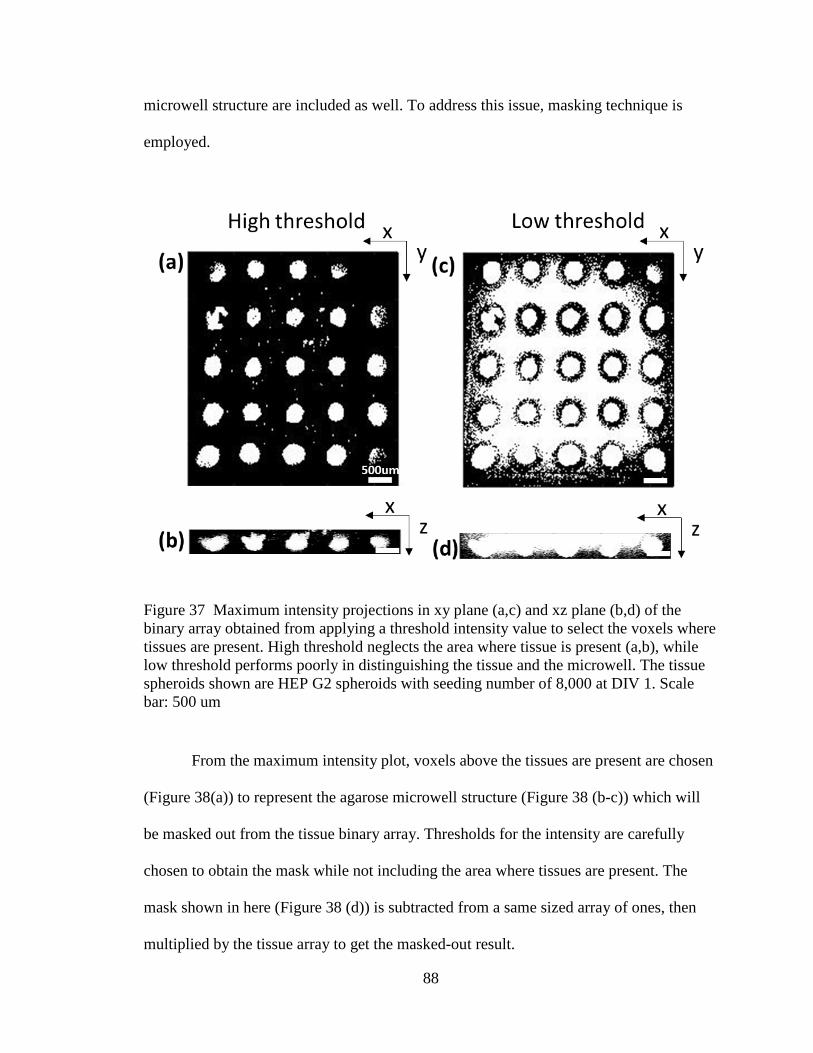
88

microwell structure are included as well. To address this issue, masking technique is

employed.

Figure 37 Maximum intensity projections in xy plane (a,c) and xz plane (b,d) of the binary array obtained from applying a threshold intensity value to select the voxels where tissues are present. High threshold neglects the area where tissue is present (a,b), while low threshold performs poorly in distinguishing the tissue and the microwell. The tissue spheroids shown are HEP G2 spheroids with seeding number of 8,000 at DIV 1. Scale bar: 500 um

From the maximum intensity plot, voxels above the tissues are present are chosen

(Figure 38(a)) to represent the agarose microwell structure (Figure 38 (b-c)) which will

be masked out from the tissue binary array. Thresholds for the intensity are carefully

chosen to obtain the mask while not including the area where tissues are present. The

mask shown in here (Figure 38 (d)) is subtracted from a same sized array of ones, then

multiplied by the tissue array to get the masked-out result.

89

Figure 38 (a) Maximum intensity projections in yz plane where users select the arrays to use as a mask. Maximum intensity projections in xy and yz planes (b,c) of the selected mask array. Binary two-dimensional array obtained from applying a threshold intensity value to select the voxels where microwell is present. The tissue spheroids shown are HEP G2 spheroids with seeding number of 8,000 at DIV 1. Scale bar: 500 um

The resulting array of the masking is shown as maximum intensity plot in Figure

39(a-b). There are still defects that are not masked out with the process. The user can

remove the unwanted defects manually by selecting rectangular area from the plot

(Figure 39 (c)), which is also achievable with y- and z- plot. Note that two tissues in the

far-right column are also manually masked. Due to confocal effect, tissues in the edge of

the field of view are sometimes not captured with the comparably high intensity as the

90

other tissues are. These tissues are removed from the array to get an accurate measure of

the data.

Figure 39 Maximum intensity projection of tissue array in xy plane (a) and xz plane (b) after masking is applied. Manual selecting of the masking shown in maximum intensity projection of tissue array in xy plane (c). The tissue spheroids shown are HEP G2 spheroids with seeding number of 8,000 at DIV 1. Scale bar: 500 um

Resulting array is shown in Figure 40 (a-b). From this binary array, number of

ones are counted and multiplied by the voxel size (20 um X 20 um X 3.46 um) to

91

calculate the volume of all tissues. The tissue counts are also recorded to obtain average

volume of the individual cell.

Figure 40 Maximum intensity projection of tissue array in xy plane (a) and xz plane (b) in final form. The tissue spheroids shown are HEP G2 spheroids with seeding number of 8,000 at DIV 1. Scale bar : 500um

Surface area is calculated by counting the differential sign change of the binary

array. Differential array of the current binary array is obtained. Differential will occur

when there is change in value, which can be interpreted as either tissue to ambient fluid

or ambient fluid to tissue, thus the surface area of the tissue. These changes are summed

and multiplied by the diagonal length of a pixel in x- and z- direction. Figure 41 shows en

face images of the differential array at 138 um from the of the top of the array, in the

center, and 138 um from the of the bottom of the array, respectively.

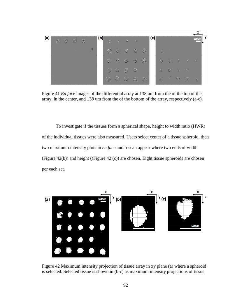
92

Figure 41 En face images of the differential array at 138 um from the of the top of the array, in the center, and 138 um from the of the bottom of the array, respectively (a-c).

To investigate if the tissues form a spherical shape, height to width ratio (HWR)

of the individual tissues were also measured. Users select center of a tissue spheroid, then

two maximum intensity plots in en face and b-scan appear where two ends of width

(Figure 42(b)) and height ((Figure 42 (c)) are chosen. Eight tissue spheroids are chosen

per each set.

Figure 42 Maximum intensity projection of tissue array in xy plane (a) where a spheroid is selected. Selected tissue is shown in (b-c) as maximum intensity projections of tissue

93

array in xy and yz planes. The two windows collect the height and width data from manual selection of the user. The tissue spheroids shown are HEP G2 spheroids with seeding number of 8,000 at DIV 1. Scale bar: 500um


Viability metric observations

Fibroblast

Diffusion coefficient and decorrelation measurement were performed with tissue

spheroids. Figure 43 shows intensity, decorrelation, and relative decorrelation of the

fibroblast tissue at the equator of three different seeding numbers. In all cases, individual

cells are not seen when the focal depth is in the equator. Cell shapes are seen in the rim of

the spheroids, where the depth of tissue for light penetration is the smallest.

94

Figure 43 Maximum intensity projection of individual spheroids with different seeding numbers in yz plane. Maximum projections of 5 neighboring layers (17.3 um) at tissue equator of intensity, decorrelation, and relative decorrelation are shown in the column below each seeding numbers. The tissue spheroids shown are fibroblast spheroids with seeding numbers of 1,000 (a-d), 4,000 (e-h), and 16,000 (i-l) at DIV 1. Scale bar: 100 um

Figure 44 shows the intensity, decorrelation, and relative decorrelation of the

same data, but at different axial position (14 pixels (47.6 um) from Figure 44(i-l)). Due to

the confocal effect, the focus is in the rim of the spheroid (Figure 44(a)). Cell shape in the

rim where the intensity is the highest appears in all metrics. Mapping of the three metrics

in retinal tissue layers (Chapter.3) demonstrated the cell existence when the penetration

depth was up to 200 um. The largest spheroid has diameter around 400 um, thus at the

equator, penetration depth is 200 um, comparable to the retinal tissue layer penetration

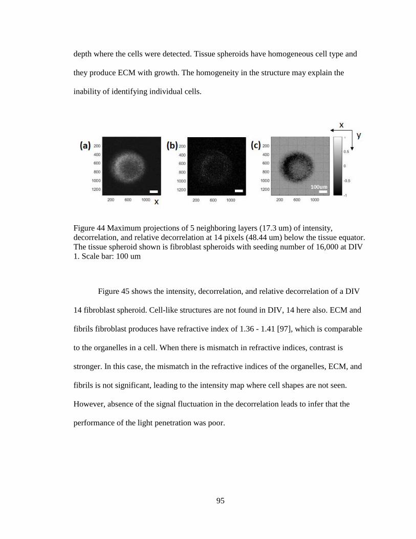
95

depth where the cells were detected. Tissue spheroids have homogeneous cell type and

they produce ECM with growth. The homogeneity in the structure may explain the

inability of identifying individual cells.

Figure 44 Maximum projections of 5 neighboring layers (17.3 um) of intensity, decorrelation, and relative decorrelation at 14 pixels (48.44 um) below the tissue equator. The tissue spheroid shown is fibroblast spheroids with seeding number of 16,000 at DIV 1. Scale bar: 100 um

Figure 45 shows the intensity, decorrelation, and relative decorrelation of a DIV

14 fibroblast spheroid. Cell-like structures are not found in DIV, 14 here also. ECM and

fibrils fibroblast produces have refractive index of 1.36 - 1.41 [97], which is comparable

to the organelles in a cell. When there is mismatch in refractive indices, contrast is

stronger. In this case, the mismatch in the refractive indices of the organelles, ECM, and

fibrils is not significant, leading to the intensity map where cell shapes are not seen.

However, absence of the signal fluctuation in the decorrelation leads to infer that the

performance of the light penetration was poor.

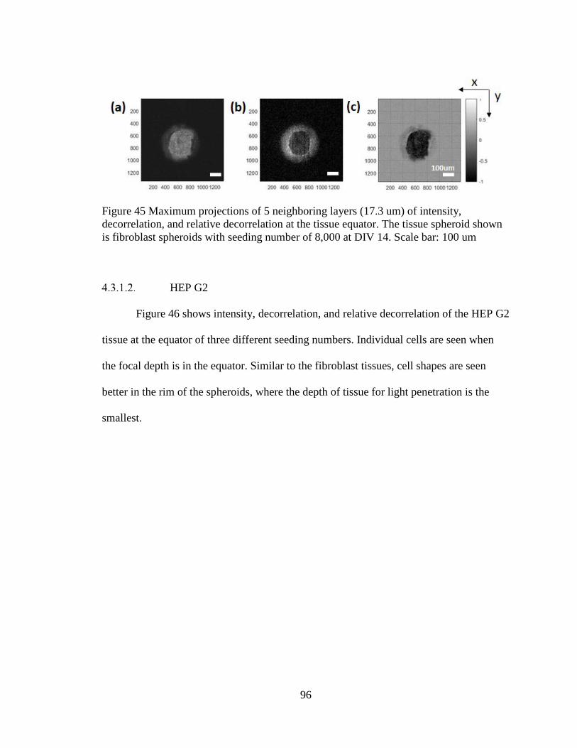
96

Figure 45 Maximum projections of 5 neighboring layers (17.3 um) of intensity, decorrelation, and relative decorrelation at the tissue equator. The tissue spheroid shown is fibroblast spheroids with seeding number of 8,000 at DIV 14. Scale bar: 100 um

HEP G2

Figure 46 shows intensity, decorrelation, and relative decorrelation of the HEP G2

tissue at the equator of three different seeding numbers. Individual cells are seen when

the focal depth is in the equator. Similar to the fibroblast tissues, cell shapes are seen

better in the rim of the spheroids, where the depth of tissue for light penetration is the

smallest.

97

Figure 46 Maximum intensity projection of individual spheroids with different seeding numbers in yz plane. Maximum projections of 5 neighboring layers (17.3 um) at tissue equator of intensity, decorrelation, and relative decorrelation are shown in the column below each seeding numbers. The tissue spheroids shown are fibroblast spheroids with seeding numbers of 1,000 (a-d), 4,000 (e-h), and 16,000 (i-l) at DIV 1. Scale bar: 100 um

HEP G2 tissues do not form a sphere, rather it forms a shape with comparatively

flat top. Figure 47 shows the intensity, decorrelation, and relative decorrelation of a DIV

1 HEP G2 spheroid. Cell shapes are detected in all three metrics at the surface.

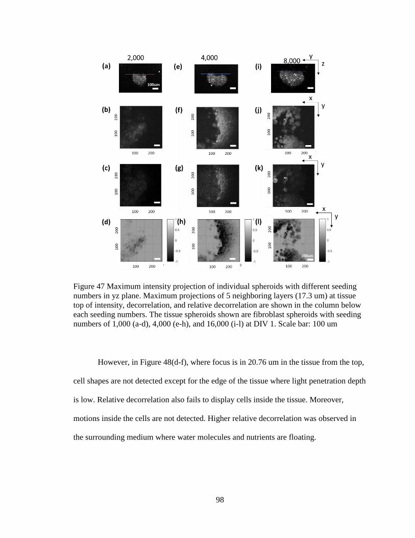
98

Figure 47 Maximum intensity projection of individual spheroids with different seeding numbers in yz plane. Maximum projections of 5 neighboring layers (17.3 um) at tissue top of intensity, decorrelation, and relative decorrelation are shown in the column below each seeding numbers. The tissue spheroids shown are fibroblast spheroids with seeding numbers of 1,000 (a-d), 4,000 (e-h), and 16,000 (i-l) at DIV 1. Scale bar: 100 um

However, in Figure 48(d-f), where focus is in 20.76 um in the tissue from the top,

cell shapes are not detected except for the edge of the tissue where light penetration depth

is low. Relative decorrelation also fails to display cells inside the tissue. Moreover,

motions inside the cells are not detected. Higher relative decorrelation was observed in

the surrounding medium where water molecules and nutrients are floating.

99

Figure 48 Maximum projections of 5 neighboring layers (17.3 um) of intensity, decorrelation, and relative decorrelation at the surface of the tissue and at 6 pixels (20.76 um) below the tissue surface. The tissue spheroid shown is HEP G2 spheroids with seeding number of 8,000 at DIV 1. Scale bar : 100 um

Morphological observations

Fibroblast Spheroids

Three different seeding numbers yielded difference in sizing, moreover, DIV 24 samples

showed difference in the shapes due to the debris around the spheroid. Figure 49 (a-b, c-

d, e-f) shows maximum intensity projections in xy and yz planes of a fibroblast spheroid

with seeding number of 1,000, 4,000, and 16,000 at DIV 1.

100

Figure 49 Maximum intensity projection of individual spheroids with different seeding numbers in xy and yz planes. The tissue spheroids shown are fibroblast spheroids with seeding numbers of 1,000 (a-b), 4,000 (c-d), and 16,000 (e-f) at DIV 1. Scale bar: 100 um

Figure 50(a-b) shows maximum intensity projections in xy and yz plane of a fibroblast

spheroid with seeding number of 16,000 and DIV 1. Figure 50 (c-d) shows maximum

intensity projections in xy and yz plane of a fibroblast spheroid with seeding number of

16,000 and DIV 14. DIV 1 spheroid is a prolate ellipsoid without any debris around the

spheroid whereas DIV 14 spheroid has a main body that is spherical and has a band around

the bottom of the spheroid that is debris from the main body.

101

Figure 50 Maximum intensity projection of individual spheroids with different DIV in xy and xz planes. The tissue spheroids shown are fibroblast spheroids with seeding numbers of 16,000 at DIV 1 (a-b) and DIV 14 (c-d). Scale bar: 100um

Surface area to volume ratio

Surface area to volume ratio (SVR) in 1/mm^3 of the fibroblast tissue spheroids of

different seeding numbers per individual tissue spheroids are shown in Fig. #. Two

separate samples of DIV 1 do behave similarly. However, there deviation is large. SVR

does not decrease linearly, due to its proportionality to the inverse of diameter of a

spheroid. To better understand the morphology of the tissue, Height to width ratio

(HWR) is measured.

102

Figure 51 Surface area to volume ratio with error bars of DIV 1 and DIV 14 samples to the seeding numbers (1,000, 4,000 and 16,000). Red and blue: DIV 1 of separate samples. Yellow: DIV 14 samples

HWR of the spheroids are plotted to investigate the shape of the spheroid. A

Perfect spheroid have HWR of 1. The HWR plotted shows that the tissues are prolate

ellipsoids except for the 2,000 spheroids with DIV 14 which may be an oblate ellipsoid.

In all seeding numbers, HWRs of DIV 14 were lower than that of DIV 1. This can be due

to the shape change (Figure 52) from having debris around the main body which became

spherical. The shapes of the tissue spheroids are determined by many factors such as

surface tension from interaction of the neighboring cells [104], the effect from

cytoskeleton [105], as well as the capability of the penetration of the nutrients. Fibroblast

103

cell type formed prolate ellipsoid in most cases to optimize the mechanical as well as

biological conditions [106].

Figure 52 Height to width ratio (HWR) to seeding numbers. The average HWR is fitted across the seeding numbers within the set of samples.

Individual tissue volume

Individual tissue volumes per each seeding numbers are plotted and fitted using least

square fit (Figure 53). Single spheroid volumes were higher in DIV 1 in larger seeding

numbers (4,000 and 16,000). Single volume for seeding number of 2,000 was higher in

older sample (DIV 14). General trend in all the set of samples showed a linear

relationship to the seeding numbers. However, the slope of the fitted lines for DIV 24

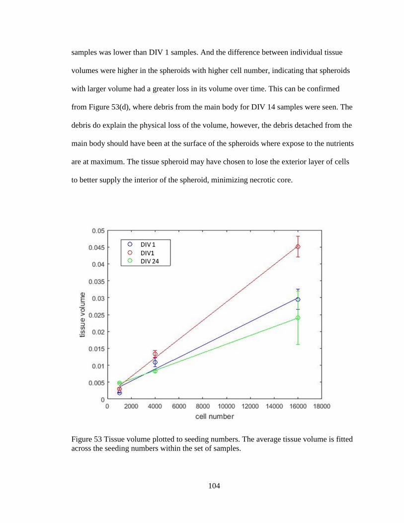
104

samples was lower than DIV 1 samples. And the difference between individual tissue

volumes were higher in the spheroids with higher cell number, indicating that spheroids

with larger volume had a greater loss in its volume over time. This can be confirmed

from Figure 53(d), where debris from the main body for DIV 14 samples were seen. The

debris do explain the physical loss of the volume, however, the debris detached from the

main body should have been at the surface of the spheroids where expose to the nutrients

are at maximum. The tissue spheroid may have chosen to lose the exterior layer of cells

to better supply the interior of the spheroid, minimizing necrotic core.

Figure 53 Tissue volume plotted to seeding numbers. The average tissue volume is fitted across the seeding numbers within the set of samples.

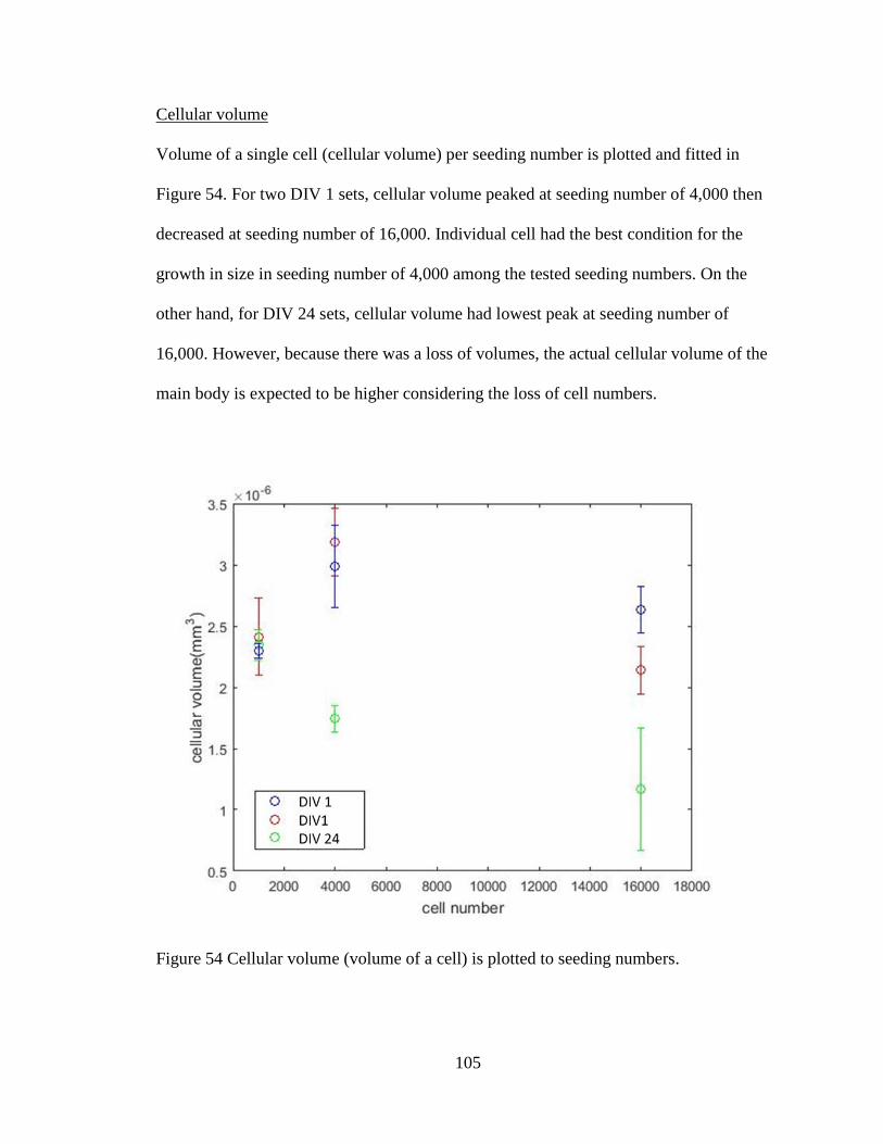
105

Cellular volume

Volume of a single cell (cellular volume) per seeding number is plotted and fitted in

Figure 54. For two DIV 1 sets, cellular volume peaked at seeding number of 4,000 then

decreased at seeding number of 16,000. Individual cell had the best condition for the

growth in size in seeding number of 4,000 among the tested seeding numbers. On the

other hand, for DIV 24 sets, cellular volume had lowest peak at seeding number of

16,000. However, because there was a loss of volumes, the actual cellular volume of the

main body is expected to be higher considering the loss of cell numbers.

Figure 54 Cellular volume (volume of a cell) is plotted to seeding numbers.

106

HEP G2 spheroids

Three different seeding numbers yielded difference in sizing. Figure 55(a-b, c-d, e-f)

shows maximum intensity projections in xy and yz planes of a fibroblast spheroid with

seeding number of 2,000, 4,000, and 8,000 at DIV 1. Hep G2 spheroids are oblate across

all the seeding numbers with a crater in the center shaping itself into a bowl-like

structure. The crater was largest in the spheroid with seeding number of 8,000.

Figure 55 Maximum intensity projection of individual spheroids with different seeding numbers in xy and yz planes. The tissue spheroids shown are HEP G2 spheroids with seeding numbers of 2,000 (a-b), 4,000 (c-d), and 8,000 (e-f) at DIV 1. Scale bar: 100um

Surface area to volume ratio

Surface area to volume ratio (SVR) in 1/mm3 of the HEP G2 tissue spheroids of different

seeding numbers per individual tissue spheroids are shown in Figure 56. SVR does not

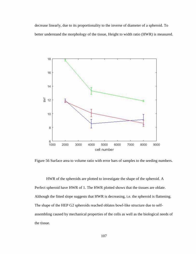
107

decrease linearly, due to its proportionality to the inverse of diameter of a spheroid. To

better understand the morphology of the tissue, Height to width ratio (HWR) is measured.

Figure 56 Surface area to volume ratio with error bars of samples to the seeding numbers.

HWR of the spheroids are plotted to investigate the shape of the spheroid. A

Perfect spheroid have HWR of 1. The HWR plotted shows that the tissues are oblate.

Although the fitted slope suggests that HWR is decreasing, i.e. the spheroid is flattening.

The shape of the HEP G2 spheroids reached oblates bowl-like structure due to self-

assembling caused by mechanical properties of the cells as well as the biological needs of

the tissue.

108

Figure 57 Height to width ratio (HWR) to seeding numbers. The average HWR is fitted across the seeding numbers within the set of samples.

Individual tissue volume

Individual tissue volumes per each seeding numbers are plotted and fitted using least

square fit (Figure 58). General trend in all the set of samples showed a linear relationship

to the seeding numbers. Slope of the fitting across different set of samples also matched.

One sample with seeding number of 4,000 behaves disparately with a very high standard

deviation.

109

Figure 58 Tissue volume (mm3) is plotted to seeding numbers. The average tissue volume is fitted across the seeding numbers within the set of samples.

Cellular volume

Volume of a single cell (cellular volume) per seeding number is plotted and fitted in

Figure 59. Cellular volume change in HEP G2 cells did not have a significant trend

within the sets of samples we measured.

110

Figure 59 Cellular volume (mm3, volume of a cell) is plotted to seeding numbers. The average cellular volume is fitted across the seeding numbers within the set of samples.

4.4. Conclusions

Two types of homogeneous tissue spheroids were studied to understand the applicability

of the SD-OCT. Our metric of interest diffusion coefficient and decorrelation was used to

quantify the viability of the tissue spheroid. Although penetrating depth of the

homogeneous tissues are comparatively low compared to the retinal tissue, the metrics

gave insights to the viability of the cells at the surface of the tissue. Further investigation

using our technique may reveal adaptable applicability. Combining this result with

111

histology and fluorescence microscopy will further guide us to the linkage of our metrics

to the conventional methods.

Morphological observation using SD-OCT revealed the adaptability for

measuring volumetric and surficial measures of the tissues. Our method of measurement

dismisses biased measurement done by directly measuring. On top of gathering the

volumetric information at once, it will further improve the accuracy of the measurements

by automating most of analysis.

Overall, measuring volumetric and surficial metric was enabled using our label-

free and noninvasive technique. Viability imaging was not as successful as ex vivo tissue,

nevertheless, it guided us in understanding the surficial cellular viability.

112

5.

CONCLUSION

113

In this study, our newly developed label-free, noninvasive technique using SD-OCT, dynamic light

scattering optical coherence tomography (DLS-OCT) was optimized and validated for accurate 3D

mapping of diffusion coefficient without any labelling. We demonstrated cellular viability imaging

of retinal neural cells and tissue spheroids, as well as volumetric and surficial measurement on

geography of tissue spheroids.

To validate that our diffusion coefficient measurement of intracellular motility

indeed represents cellular viability, we triggered the change of the health in the sample by

changing the environmental conditions and releasing certain chemicals known to affect the

organelles and the structure of the cytoplasm. We saw change when such change was

induced, when the condition change to the viability was mild, the diffusion coefficient

change was also subtle. When change to the viability was harsh, the diffusion coefficient

change was also large. Further study in linking the cytoplasmic change known with the

diffusion coefficient will guide us in understanding the motional change each cytoplasmic

change induces. Decorrelation was also studied using various conditions induced.

Diffusion coefficient and decorrelation change (relative decorrelation, specifically) have

similarity although the absolute comparison was not available. Here, intracellular motility

(IM) was quantitatively imaged with cellular resolution through scattering tissue and

validated to represent cellular viability.

Measurement of geographical and volumetric metric of tissues is also promising in

that it is done without destructing the tissues. Using our technique, longitudinal study of

specific tissue spheroids will be possible. This will fortify the observations we saw

114

statistically. Similar to biological tissue, when viability was manipulated, IM exhibited a

decrease as expected from the known effect. In addition, morphological measurement using

SD-OCT revealed the adaptability for measuring volumetric and surficial measures of the

tissues. Therefore, it can be concluded that the viability of the engineered tissue can also

be assessed through IM as well as morphological measurement.

To Conclude, this research has addressed the current limitations in the existing methods

for tissue viability assessment. The technique developed through and findings obtained

from this research are expected to address the need to nondestructively measure the

viability of biological and engineered tissue. Such nondestructive viability assessment

will have a range of applications, from disease studies to drug discovery and tissue

production.

115

REFERENCES

1. R. M. Berne, B. M. Koeppen, and B. A. Stanton, Berne & Levy Physiology

(Mosby/Elsevier, 2010).

2. O. Kepp, L. Galluzzi, M. Lipinski, J. Yuan, and G. Kroemer, "Cell death assays for

drug discovery," Nat. Rev. Drug Discov. 10, 221–237 (2011).

3. D. T. Vistica, P. Skehan, D. Scudiero, A. Monks, A. Pittman, and M. R. Boyd,

"Tetrazolium-based Assays for Cellular Viability: A Critical Examination of

Selected Parameters Affecting Formazan Production," CANCER Res. 51, 2515–

2520 (1991).

4. S. R. Khetani and S. N. Bhatia, "Microscale culture of human liver cells for drug

development," Nat. Biotechnol. 26, 120–126 (2008).

5. A. Ridley and R. Heald, "Cell structure and dynamics," Curr. Opin. Cell Biol. 23,

1–3 (2011).

6. C. M. Waterman-Storer and E. D. Salmon, "Actomyosin-based Retrograde Flow of

Microtubules in the Lamella of Migrating Epithelial Cells Influences Microtubule

Dynamic Instability and Turnover and Is Associated with Microtubule Breakage and

Treadmilling," J. Cell Biol. 139, 417–434 (1997).

7. C. Joo, C. L. Evans, T. Stepinac, T. Hasan, and J. F. de Boer, "Diffusive and

directional intracellular dynamics measured by field-based dynamic light

scattering," Opt. Express 18, 2858 (2010).

116

8. K. Jacobson and J. Wojcieszyn, "The translational mobility of substances within the

cytoplasmic matrix.," Proc. Natl. Acad. Sci. U. S. A. 81, 6747–6751 (1984).

9. P. A. Valberg and H. A. Feldman, "Magnetic particle motions within living cells.

Measurement of cytoplasmic viscosity and motile activity.," Biophys. J. 52, 551–61

(1987).

10. D. Merrill, R. An, J. Turek, and D. D. Nolte, "Digital holography of intracellular

dynamics to probe tissue physiology.," Appl. Opt. 54, A89-97 (2015).

11. P. A. Valberg and D. F. Albertini, "Cytoplasmic motions, rheology, and structure

probed by a novel magnetic particle method.," J. Cell Biol. 101, 130–40 (1985).

12. D. D. Nolte, R. An, J. Turek, and K. Jeong, "Holographic tissue dynamics

spectroscopy.," J. Biomed. Opt. 16, 87004 (2011).

13. B. Herman, "A time-lapse video image intensification analysis of cytoplasmic

organelle movements during endosome translocation," J. Cell Biol. 98, 565–576

(1984).

14. C. P. Brangwynne, F. C. MacKintosh, and D. A. Weitz, "Force fluctuations and

polymerization dynamics of intracellular microtubules.," Proc. Natl. Acad. Sci. U.

S. A. 104, 16128–33 (2007).

15. Y. Tseng, T. P. Kole, and D. Wirtz, "Micromechanical mapping of live cells by

multiple-particle-tracking microrheology," Biophys. J. 83, 3162–3176 (2002).

16. P. Panorchan, J. S. H. Lee, T. P. Kole, Y. Tseng, and D. Wirtz, "Microrheology and

ROCK signaling of human endothelial cells embedded in a 3D matrix.," Biophys. J.

91, 3499–507 (2006).

117

17. K. Luby-phelps, P. E. Castles, D. L. Taylort, and F. Lannit, "Hindered diffusion of

inert tracer particles in the cytoplasm of mouse 3T3 cells," 84, 4910–4913 (1987).

18. K. Luby-Phelps, D. L. Taylor, and F. Lanni, "Probing the structure of cytoplasm," J.

Cell Biol. 102, 2015–2022 (1986).

19. E. L. Elson and D. Magde, "Fluorescence correlation spectroscopy. I. Conceptual

basis and theory," Biopolymers 13, 1–27 (1974).

20. H. Chen, E. R. Farkas, and W. W. Webb, "Chapter 1 In Vivo Applications of

Fluorescence Correlation Spectroscopy," Methods Cell Biol. 89, 3–35 (2008).

21. M. Prummer, D. Kling, V. Trefzer, T. Enderle, S. Zoffmann, and M. Prunotto, "A

random motility assay based on image correlation spectroscopy.," Biophys. J. 104,

2362–72 (2013).

22. M. Guo, A. J. Ehrlicher, M. H. Jensen, M. Renz, J. R. Moore, R. D. Goldman, J.

Lippincott-Schwartz, F. C. Mackintosh, and D. A. Weitz, "Probing the stochastic,

motor-driven properties of the cytoplasm using force spectrum microscopy," Cell

158, 822–832 (2014).

23. A. L. Oldenburg, R. K. Chhetri, J. M. Cooper, W.-C. Wu, M. A. Troester, and J. B.

Tracy, "Motility-, autocorrelation-, and polarization-sensitive optical coherence

tomography discriminates cells and gold nanorods within 3D tissue cultures," Opt.

Lett. 38, 2923 (2013).

24. A. L. Oldenburg, X. Yu, T. Gilliss, O. Alabi, R. M. Taylor, and M. A. Troester,

"Inverse-power-law behavior of cellular motility reveals stromal–epithelial cell

interactions in 3D co-culture by OCT fluctuation spectroscopy," Optica 2, 877

118

(2015).

25. C. Apelian, F. Harms, O. Thouvenin, and A. C. Boccara, "Dynamic full field optical

coherence tomography: subcellular metabolic contrast revealed in tissues by

interferometric signals temporal analysis," Biomed. Opt. Express 7, 1511 (2016).

26. N. T. Shaked and A. Wax, "Quantitative Phase Microscopy of Live Biological Cell

Dynamics," in Advanced Phase Measurement Methods in Optics and Imaging

(Springer Berlin Heidelberg, 2010), pp. 283–288.

27. G. Popescu, Y. Park, W. Choi, R. R. Dasari, M. S. Feld, and K. Badizadegan,

"Imaging red blood cell dynamics by quantitative phase microscopy," Blood Cells,

Mol. Dis. 41, 10–16 (2008).

28. T. Yamauchi, H. Iwai, and Y. Yamashita, "Label-free imaging of intracellular

motility by low-coherent quantitative phase microscopy," Opt. Express 19, 5536

(2011).

29. D. B. Sattelle, D. J. Green, and K. H. Langley, "Subcellular Motions in Nitella

flexilis studied by Photon Correlation Spectroscopy," Phys. Scr. 19, 471–475 (1979).

30. J. Lee, W. Wu, J. Y. Jiang, B. Zhu, and D. A. Boas, "Dynamic light scattering optical

coherence tomography," Opt. Express 20, 22262–22277 (2012).

31. J. Lee, H. Radhakrishnan, W. Wu, A. Daneshmand, M. Climov, C. Ayata, and D. A.

Boas, "Quantitative imaging of cerebral blood flow velocity and intracellular

motility using dynamic light scattering-optical coherence tomography," J. Cereb.

Blood Flow Metab. 33, 819–825 (2013).

32. S. Marlar, E. C. Arnspang, G. A. Pedersen, J. S. Koffman, and L. N. Nejsum,

119

"Measuring localization and diffusion coefficients of basolateral proteins in lateral

versus basal membranes using functionalized substrates and kICS analysis,"

Biochim. Biophys. Acta - Biomembr. 1838, 2404–2411 (2014).

33. a I. García-Pérez, E. A. López-Beltrán, P. Klüner, J. Luque, P. Ballesteros, and S.

Cerdán, "Molecular crowding and viscosity as determinants of translational

diffusion of metabolites in subcellular organelles.," Arch. Biochem. Biophys. 362,

329–38 (1999).

34. J. W. Wojcieszyn, R. A. Schlegelt, E.-S. Wut, and K. A. Jacobson, "Diffusion of

injected macromolecules within the cytoplasm of living cells (erythrocyte-mediated

microinjection/photobleaching/human fibroblast/cytoplasmic

viscosity/cytoskeleton)," Cell Biol. 78, 4407–4410 (1981).

35. G. L. Lukacs, P. Haggie, O. Seksek, D. Lechardeur, N. Freedman, and A. S.

Verkman, "Size-dependent DNA mobility in cytoplasm and nucleus," J. Biol. Chem.

275, 1625–1629 (2000).

36. R. Brock, M. A. Hink, and T. M. Jovin, "Fluorescence correlation microscopy of

cells in the presence of autofluorescence.," Biophys. J. 75, 2547–57 (1998).

37. S. Yazdanfar, A. M. Rollins, and J. A. Izatt, "In Vivo Imaging of Human Retinal

Flow Dynamics by Color Doppler Optical Coherence Tomography," Arch.

Ophthalmol. 121, 235 (2003).

38. J. A. Izatt, M. D. Kulkarni, S. Yazdanfar, J. K. Barton, and A. J. Welch, "In vivo

bidirectional color Doppler flow imaging of picoliter blood volumes using optical

coherence tomography," Opt. Lett. 22, 1439 (1997).

120

39. Y. Chen, A. D. Aguirre, L. Ruvinskaya, A. Devor, D. A. Boas, and J. G. Fujimoto,

"Optical coherence tomography (OCT) reveals depth-resolved dynamics during

functional brain activation," J. Neurosci. Methods 178, 162–173 (2009).

40. S. B. Ploner, E. M. Moult, W. Choi, N. K. Waheed, B. Lee, E. A. Novais, E. D. Cole,

B. Potsaid, L. Husvogt, J. Schottenhamml, A. Maier, P. J. Rosenfeld, J. S. Duker, J.

Hornegger, and J. G. Fujimoto, "TOWARD QUANTITATIVE OPTICAL

COHERENCE TOMOGRAPHY ANGIOGRAPHY," Retina 36, S118–S126 (2016).

41. D. Jaque, L. Martínez Maestro, B. del Rosal, P. Haro-Gonzalez, A. Benayas, J. L.

Plaza, E. Martín Rodríguez, J. García Solé, B. Hildebrandt, P. Wust, O. Ahlers, A.

Dieing, G. Sreenivasa, T. Kerner, R. Felix, H. Riess, J. L. R. Roti, A. Chicheł, J.

Skowronek, M. Kubaszewska, M. Kanikowski, P. Wust, B. Hildebrandt, G.

Sreenivasa, B. Rau, J. Gellermann, H. Riess, R. Felix, P. M. Schlag, A. Burlaka, S.

Lukin, S. Prylutska, O. Remeniak, Y. Prylutskyy, M. Shuba, S. Maksimenko, U.

Ritter, P. Scharff, N. P. O’Grady, P. S. Barie, J. G. Bartlett, T. Bleck, G. Garvey, J.

Jacobi, P. Linden, D. G. Maki, M. Nam, W. Pasculle, J. Van der Zee, R. W. Habash,

R. Bansal, D. Krewski, H. T. Alhafid, R. W. Habash, R. Bansal, D. Krewski, H. T.

Alhafid, M. Johannsen, U. Gneveckow, L. Eckelt, A. Feussner, N. Waldofner, R.

Scholz, S. Deger, P. Wust, S. A. Loening, A. Jordan, J. Mendecki, E. Friedenthal,

C. Botstein, R. Paglione, F. Sterzer, G. Hegyi, G. P. Szigeti, A. Szasz, F. Zhou, D.

Xing, Z. Ou, B. Wu, D. E. Resasco, W. R. Chen, J. W. Fisher, S. Sarkar, C. F.

Buchanan, C. S. Szot, J. Whitney, H. C. Hatcher, S. V. Torti, C. G. Rylander, M. N.

Rylander, T. Hironobu, N. Takuro, N. Ayuko, N. Yasuro, Y. Sunao, C. W. Song, S.

S. Chen, J. Humphrey, J. R. Oleson, T. V. Samulski, K. A. Leopold, S. T. Clegg, M.

121

W. Dewhirst, R. K. Dodge, S. L. George, R. W. Habash, R. Bansal, D. Krewski, H.

T. Alhafid, P. Chakravarty, R. Marches, N. S. Zimmerman, A. D. Swafford, P. Bajaj,

I. H. Musselman, P. Pantano, R. K. Draper, E. S. Vitetta, R. W. Habash, R. Bansal,

D. Krewski, H. T. Alhafid, S. V. Torti, F. Byrne, O. Whelan, N. Levi, B. Ucer, M.

Schmid, F. M. Torti, S. Akman, J. Liu, P. M. Ajayan, O. Nalamasu, D. L. Carroll,

S. N. Goldberg, M. C. Stein, G. S. Gazelle, R. G. Sheiman, J. B. Kruskal, M. E.

Clouse, C. J. Diederich, T. Corwin, G. Lindberg, O. Traxer, M. T. Gettman, T. G.

Smith, M. S. Pearle, J. A. Cadeddu, F. Litvack, W. S. Grundfest, T. Papaioannou, F.

W. Mohr, A. T. Jakubowski, J. S. Forrester, S. Rastegar, M. Motamedi, A. J. Welch,

L. J. Hayes, A. J. Welch, M. Motamedi, S. Rastegar, G. L. Lecarpentier, D. Jansen,

S. A. Sapareto, W. C. Dewey, A. Busetti, M. Soncin, E. Reddi, M. A. Rodgers, M.

E. Kenney, G. Jori, J. R. Lepock, K.-H. Cheng, H. Al-qysi, I. Sim, C. J. Koch, J.

Kruuv, J. R. Lepock, H. E. Frey, A. M. Rodahl, J. Kruuv, A. E. Caccamo, S.

Desenzani, L. Belloni, A. F. Borghetti, S. Bettuzzi, K. J. Henle, L. A. Dethlefsen, B.

W. Henderson, V. H. Fingar, M. Ahmed, L. E. Gerweck, V. K. Pustovalov, L. G.

Astafyeva, W. Fritzsche, M. P. V. Shekhar, C. L. Garrett, D. O. Draper, K. L. Knight,

N. A. Armar, G. C. L. Lachelin, U. G. Longo, M. Ronga, N. Maffulli, H. I. Bicher,

F. W. Hetzel, T. S. Sandhu, S. Frinak, P. Vaupel, M. O’Hara, T. O’Brien, J. G. Short,

P. F. Turner, A. I. Minchinton, I. F. Tannock, S. H. van Rijt, P. J. Sadler, Y. Lee, S.

L. Auh, Y. Wang, B. Burnette, Y. Wang, Y. Meng, M. Beckett, R. Sharma, R. Chin,

T. Tu, A. A. Lugade, J. P. Moran, S. A. Gerber, R. C. Rose, J. G. Frelinger, E. M.

Lord, T. J. Dougherty, C. J. Gomer, B. W. Henderson, G. Jori, D. Kessel, M.

Korbelik, J. Moan, Q. Peng, M. P. Carey, T. G. Burish, J. E. Johnson, L. M. Nail, D.

122

Lauver, K. B. King, H. Keys, M. Clarke, R. Collins, S. Darby, C. Davies, P.

Elphinstone, E. Evans, J. Godwin, R. Gray, C. Hicks, S. James, I. Takahashi, Y. Emi,

S. Hasuda, Y. Kakeji, Y. Maehara, K. Sugimachi, E. L. Jones, J. R. Oleson, L. R.

Prosnitz, T. V. Samulski, Z. Vujaskovic, D. Yu, L. L. Sanders, M. W. Dewhirst, J.

B. Marmor, D. Pounds, T. B. Postic, G. M. Hahn, L. O. Svaasand, T. Boerslid, M.

Oeveraasen, A. Y. Cheung, A. Neyzari, W. Hurter, F. Reinbold, W. Lorenz, J.

Delannoy, D. LeBihan, D. Hoult, R. Levin, B. S. Trembly, B. E. Lyons, R. H. Britt,

J. W. Strohbehn, M. Johannsen, B. Thiesen, P. Wust, A. Jordan, M. Salloum, R. Ma,

D. Weeks, L. Zhu, G. Kong, R. D. Braun, M. W. Dewhirst, S. Mornet, S. Vasseur,

F. Grasset, E. Duguet, Q. A. Pankhurst, J. Connolly, S. Jones, J. Dobson, R. Hergt,

S. Dutz, R. Müller, M. Zeisberger, B. Thiesen, A. Jordan, A. Ito, M. Shinkai, H.

Honda, T. Kobayashi, R. K. Gilchrist, R. Medal, W. D. Shorey, R. C. Hanselman, J.

C. Parrott, C. B. Taylor, M. Johannsen, U. Gneveckow, K. Taymoorian, B. Thiesen,

N. Waldofner, R. Scholz, K. Jung, A. Jordan, P. Wust, S. A. Loening, B. A. Moffat,

G. R. Reddy, P. McConville, D. E. Hall, T. L. Chenevert, R. R. Kopelman, M.

Philbert, R. Weissleder, A. Rehemtulla, B. D. Ross, D. Pissuwan, S. M. Valenzuela,

M. B. Cortie, X. H. Huang, P. K. Jain, I. H. El-Sayed, M. A. El-Sayed, X. Huang, I.

H. El-Sayed, W. Qian, M. A. El-Sayed, P. K. Jain, X. Huang, I. H. El-Sayed, M. A.

El-Sayed, A. M. Smith, M. C. Mancini, S. Nie, R. Weissleder, K. König, F.

Helmchen, W. Denk, M. P. Melancon, M. Zhou, C. Li, G. S. Terentyuk, G. N.

Maslyakova, L. V. Suleymanova, N. G. Khlebtsov, B. N. Khlebtsov, M. Olivo, C.

Y. Fu, V. Raghavan, W. K. Lau, M. A. Albota, C. Xu, W. W. Webb, J. G.

Teeguarden, P. M. Hinderliter, G. Orr, B. D. Thrall, J. G. Pounds, M. S. Nikolic, M.

123

Krack, V. Aleksandrovic, A. Kornowski, S. Förster, H. Weller, X. Shi, S. Wang, H.

Sun, J. R. Baker, W. W. Yu, E. Chang, R. Drezek, V. L. Colvin, N. R. Jana, C.

Earhart, J. Y. Ying, J. -s. Choi, Y. -w. Jun, S.-I. Yeon, H. C. Kim, J.-S. Shin, J.

Cheon, X. Hong, Z. Wang, W. Cai, F. Lu, J. Zhang, Y. Yang, N. Ma, Y. Liu, J. R.

McCarthy, E. Korngold, R. Weissleder, F. A. Jaffer, A. Barhoumi, R. Huschka, R.

Bardhan, M. W. Knight, N. J. Halas, U. Rocha, K. U. Kumar, C. Jacinto, I. Villa, F.

Sanz-Rodríguez, M. del C. I. de la Cruz, A. Juarranz, E. Carrasco, F. C. J. M. van

Veggel, E. Bovero, J. G. Solé, D. Jaque, H. Huang, S. Delikanli, H. Zeng, D. M.

Ferkey, A. Pralle, L. Cheng, K. Yang, Q. Chen, Z. Liu, L. M. Maestro, P. Haro-

Gonzalez, B. del Rosal, J. Ramiro, A. J. Caamano, E. Carrasco, A. Juarranz, F. Sanz-

Rodriguez, J. G. Sole, D. Jaque, S. Link, M. A. El-Sayed, S. Link, M. A. El-Sayed,

G. Mie, J. F. Lovell, C. S. Jin, E. Huynh, H. Jin, C. Kim, S. K. Ghosh, T. Pal, P. K.

Jain, I. H. El-Sayed, M. A. El-Sayed, S. E. Skrabalak, J. Chen, L. Au, X. Lu, X. Li,

Y. Xia, E. Carbo-Argibay, B. Rodriguez-Gonzalez, J. Pacifico, I. Pastoriza-Santos,

J. Perez-Juste, L. M. Liz-Marzan, J. Pérez-Juste, I. Pastoriza-Santos, L. M. Liz-

Marzán, P. Mulvaney, P. K. Jain, K. S. Lee, I. H. El-Sayed, M. A. El-Sayed, L.

Maestro, P. Haro-González, J. Coello, D. Jaque, E. Prodan, P. Nordlander, N. J.

Halas, S. J. Oldenburg, J. B. Jackson, S. L. Westcott, N. J. Halas, A. M. Fales, H.

Yuan, T. Vo-Dinh, R. Rodríguez-Oliveros, J. A. Sánchez-Gil, H. Yuan, C. G.

Khoury, C. M. Wilson, G. A. Grant, A. J. Bennett, T. Vo-Dinh, S. Trigari, A. Rindi,

G. Margheri, S. Sottini, G. Dellepiane, E. Giorgetti, J. Chen, B. Wiley, Z. Y. Li, D.

Campbell, F. Saeki, H. Cang, L. Au, J. Lee, X. Li, Y. Xia, M. F. Tsai, S. H. Chang,

F. Y. Cheng, V. Shanmugam, Y. S. Cheng, C. H. Su, C. S. Yeh, Y. Jin, J. Wang, H.

124

Ke, S. Wang, Z. Dai, H. Ke, J. Wang, Z. Dai, Y. Jin, E. Qu, Z. Xing, C. Guo, X.

Yue, J. Liu, H. Ke, J. Wang, S. Tong, Y. Jin, S. Wang, E. Qu, G. Bao, Z. Dai, H. Ke,

X. Yue, J. Wang, S. Xing, Q. Zhang, Z. Dai, J. Tian, S. Wang, Y. Jin, S. C. Boca,

M. Potara, A. M. Gabudean, A. Juhem, P. L. Baldeck, S. Astilean, G. Fu, W. Liu, S.

Feng, X. Yue, M. Shokouhimehr, E. S. Soehnlen, A. Khitrin, S. Basu, S. P. D. Huang,

M. Shokouhimehr, E. S. Soehnlen, J. H. Hao, M. Griswold, C. Flask, X. D. Fan, J.

P. Basilion, S. Basu, S. P. D. Huang, N. H. Levi-Polyachenko, E. J. Merkel, B. T.

Jones, D. L. Carroll, J. H. Stewart, S. J. Yu, M. W. Kang, H. C. Chang, K. M. Chen,

Y. C. Yu, G. Kucsko, P. C. Maurer, N. Y. Yao, M. Kubo, H. J. Noh, S. Iijima, J. T.

Robinson, S. M. Tabakman, Y. Y. Liang, H. L. Wang, H. S. Casalongue, D. Vinh,

H. J. Dai, X. Sun, Z. Liu, K. Welsher, J. Robinson, A. Goodwin, S. Zaric, H. Dai, F.

Wang, G. Dukovic, L. E. Brus, T. F. Heinz, M. S. Strano, S. K. Doorn, E. H. Haroz,

C. Kittrell, R. H. Hauge, R. E. Smalley, L. Van Hove, T. Stöckli, Z. L. Wang, J. M.

Bonard, P. Sadelmann, A. Chatelain, A. V. Naumov, S. Ghosh, D. A. Tsyboulski, S.

M. Bachilo, R. B. Weisman, M. J. O’Connell, S. M. Bachilo, C. B. Huffman, V. C.

Moore, M. S. Strano, E. H. Haroz, K. L. Rialon, P. J. Boul, W. H. Noon, C. Kittrell,

J. Ma, R. H. Hauge, R. B. Weisman, R. E. Smalley, F. Wang, G. Dukovic, L. E.

Brus, T. F. Heinz, J. Crochet, M. Clemens, T. Hertel, S.-Y. Ju, W. P. Kopcha, F.

Papadimitrakopoulos, M. Lin, K. W. K. Shung, B. Zhao, M. E. Itkis, S. Niyogi, H.

Hu, J. Zhang, R. C. Haddon, F. Schöppler, C. Mann, T. C. Hain, F. M. Neubauer, G.

Privitera, F. Bonaccorso, D. Chu, A. C. Ferrari, T. Hertel, Q. Cheng, S. Debnath, E.

Gregan, H. J. Byrne, A. Burke, X. Ding, R. Singh, R. A. Kraft, N. Levi-Polyachenko,

M. N. Rylander, C. Szot, C. Buchanan, J. Whitney, J. Fisher, H. C. Hatcher, J. R.

125

D’Agostino, N. D. Kock, P. M. Ajayan, D. L. Carroll, S. Akman, F. M. Torti, S. V.

Torti, S. H. Jeong, K. K. Kim, S. J. Jeong, K. H. An, S. H. Lee, Y. H. Lee, S. H.

Kim, G. W. Mulholland, M. R. Zachariah, L. M. Maestro, E. M. Rodriguez, F.

Vetrone, R. Naccache, H. L. Ramirez, D. Jaque, J. A. Capobianco, J. G. Solé, I. L.

Medintz, H. T. Uyeda, E. R. Goldman, H. Mattoussi, N. Lewinski, V. Colvin, R.

Drezek, K. T. Yong, W. C. Law, R. Hu, L. Ye, L. Liu, M. T. Swihart, P. N. Prasad,

L. M. Maestro, P. Haro-González, M. C. I. la Cruz, F. SanzRodríguez, Á. Juarranz,

J. G. Solé, D. Jaque, S. B. Lakshmanan, X. Zou, M. Hossu, L. Ma, C. Yang, W.

Chen, Q. Tian, M. Tang, Y. Sun, R. Zou, Z. Chen, M. Zhu, S. Yang, J. Wang, J.

Wang, J. Hu, A. M. Derfus, W. C. W. Chan, S. N. Bhatia, Y. Li, W. Lu, Q. Huang,

C. Li, W. Chen, V. M. García, P. K. Nair, M. T. S. Nair, C. M. Hessel, V. P. Pattani,

M. Rasch, M. G. Panthani, B. Koo, J. W. Tunnell, B. A. Korgel, Y. Zhao, H. Pan,

Y. Lou, X. Qiu, J. Zhu, C. Burda, J. M. Luther, P. K. Jain, T. Ewers, A. P. Alivisatos,

T. N. Lambert, N. L. Andrews, H. Gerung, T. J. Boyle, J. M. Oliver, B. S. Wilson,

S. M. Han, G. Chen, T. Y. Ohulchanskyy, S. Liu, W.-C. Law, F. Wu, M. T. Swihart,

H. Ågren, P. N. Prasad, G. Chen, J. Shen, T. Y. Ohulchanskyy, N. J. Patel, A.

Kutikov, Z. Li, J. Song, R. K. Pandey, H. Ågren, P. N. Prasad, G. Han, F. Vetrone,

R. Naccache, A. J. de la Fuente, F. Sanz-Rodriguez, A. Blazquez-Castro, E. M.

Rodriguez, D. Jaque, J. G. Sole, J. A. Capobianco, D. Jaque, F. Vetrone, A. Gnach,

A. Bednarkiewicz, A. A. Ansari, S. P. Singh, N. Singh, B. D. Malhotra, D.

Wawrzynczyk, A. Bednarkiewicz, M. Nyk, W. Strek, M. Samoc, A. Bednarkiewicz,

D. Wawrzynczyk, M. Nyk, W. Strek, V. K. Tikhomirov, K. Driesen, V. D.

Rodriguez, P. Gredin, M. Mortier, U. Rocha, C. J. da Silva, W. F. Silva, I. Guedes,

126

A. Benayas, L. M. Maestro, M. A. Elias, E. Bovero, F. C. J. M. van Veggel, J. A. G.

Solé, D. Jaque, M. Ge, J. Rong, X. Fang, A. Zhang, Y. Lu, C. Zhou, A. G. Cullis, L.

T. Canham, P. D. J. Calcott, S. P. Low, N. H. Voelcker, L. T. Canham, K. A.

Williams, L. Xiao, L. Gu, S. B. Howell, M. J. Sailor, E. J. Anglin, L. Cheng, W. R.

Freeman, M. J. Sailor, E. Secret, K. Smith, V. Dubljevic, E. Moore, P. Macardle, B.

Delalat, M. L. Rogers, T. G. Johns, J. O. Durand, F. Cunin, N. H. Voelcker, J.-H.

Park, L. Gu, G. von Maltzahn, E. Ruoslahti, S. N. Bhatia, M. J. Sailor, D. Gallach,

G. R. Sánchez, A. M. Noval, M. M. Silván, G. Ceccone, R. J. M. Palma, V. T. Costa,

J. M. M. Duart, C. Lee, H. Kim, C. Hong, M. Kim, S. S. Hong, D. H. Lee, W. I. Lee,

C. Lee, C. Hong, J. Lee, M. Son, S.-S. Hong, I. Sagnes, A. Halimaoui, G. Vincent,

P. A. Badoz, J. Yu, D. Javier, M. A. Yaseen, N. Nitin, R. Richards-Kortum, J. Yang,

J. Choi, D. Bang, E. Kim, E. K. Lim, H. Park, J. S. Suh, K. Lee, K. H. Yoo, E. K.

Kim, Y. M. Huh, S. Haam, S. Sharifi, S. Behzadi, S. Laurent, M. L. Forrest, P.

Stroeve, H. Shinohara, A. Tanaka, T. Kitai, N. Yanabu, T. Inomoto, M. Zheng, C.

Yue, Y. Ma, P. Gong, P. Zhao, C. Zheng, Z. Sheng, P. Zhang, Z. Wang, L. Cai, B.

Jung, A. L. N. Rao, B. Anvari, S. Gupta, M. R. Chatni, A. L. N. Rao, V. I. Vullev,

L. V. Wang, B. Anvari, B. Bahmani, D. Bacon, B. Anvari, Y. Ma, S. Tong, G. Bao,

C. Gao, Z. Dai, C.-Y. Li, W.-Y. Chiu, C.-F. Lee, O. P. Dimitriev, L. Cheng, W. He,

H. Gong, C. Wang, Q. Chen, Z. Cheng, Z. Liu, M. Soncin, A. Busetti, F. Fusi, G.

Jori, M. A. J. Rodgers, C. S. Jin, J. F. Lovell, J. Chen, G. Zheng, L. M. Maestro, P.

Haro-González, A. Sánchez-Iglesias, L. M. Liz-Marzán, J. A. G. Sole, D. Jaque, Z.

Zha, X. Yue, Q. Ren, Z. Dai, Z. Zha, J. Wang, S. Zhang, S. Wang, E. Qu, Y. Zhang,

Z. Dai, Y. Ma, X. Liang, S. Tong, G. Bao, Q. Ren, Z. Dai, J. Turkevich, P. C.

127

Stevenson, J. Hillier, G. Frens, W. S. Sutherland, J. D. Winefordner, K. C. Grabar,

R. G. Freeman, M. B. Hommer, M. J. Natan, Z. Liang, J. Zhang, L. Wang, S. Song,

C. Fan, M. Brust, M. Walker, D. Bethell, D. J. Schiffrin, R. Whyman, J. L. Plaza, V.

Carcelen, X. Wang, J. Zhuang, Q. Peng, Y. D. Li, C. J. Murphy, N. R. Jana, B.

Nikoobakht, M. A. El-Sayed, E. B. Dickerson, E. C. Dreaden, X. H. Huang, I. H.

El-Sayed, H. H. Chu, S. Pushpanketh, J. F. McDonald, M. A. El-Sayed, F. M.

Veronese, G. Pasut, J. R. Cole, N. A. Mirin, M. W. Knight, G. P. Goodrich, N. J.

Halas, G. P. Goodrich, L. Bao, K. Gill-Sharp, K. L. Sang, J. Wang, Q. Zhang, W.

Li, L. P. Wen, J. Chen, Y. Xia, S. E. Skrabalak, J. Chen, Y. Sun, X. Lu, L. Au, J.

Chen, M. Yang, Q. Zhang, E. C. Cho, C. M. Cobley, C. Kim, C. Glaus, L. V. Wang,

M. J. Welch, Y. Xia, M. Hu, J. Chen, Z.-Y. Li, L. Au, G. V. Hartland, X. Li, M.

Marquez, Y. Xia, C. Journet, W. K. Maser, P. Bernier, A. Loiseau, M. L.

delaChapelle, M. C. Altay, S. Eroglu, T. Guo, P. Nikolaev, A. Thess, D. T. Colbert,

R. E. Smalley, M. Paradise, T. Goswami, H. Dai, Y. Uemura, K. Baba, H. Ohe, Y.

Ohzuno, Y. Hatate, A.-C. Dupuis, S. McCaldin, M. Bououdina, D. M. Grant, G. S.

Walker, A. Thess, R. Lee, P. Nikolaev, H. J. Dai, P. Petit, A. Valizadeh, H. Mikaeili,

M. Samiei, S. M. Farkhani, N. Zarghami, M. Kouhi, A. Akbarzadeh, S. Davaran, D.

Bera, L. Qian, T.-K. Tseng, P. H. Holloway, L. Y. Zhang, L. Wen, J. J. Zhang, L. L.

Hu, N. Bogdan, E. M. Rodriguez, F. Sanz-Rodriguez, M. C. I. de la Cruz, A.

Juarranz, D. Jaque, J. G. Sole, J. A. Capobianco, V. Mahalingam, F. Vetrone, R.

Naccache, A. Speghini, J. A. Capobianco, W. Zhang, Z. Guo, D. Huang, Z. Liu, X.

Guo, H. Zhong, X. Teng, Y. Zhu, W. Wei, S. Wang, J. Huang, R. Naccache, W. Hu,

A. I. Y. Tok, Y. Han, Q. Zhang, Q. Fan, W. Huang, J. A. Capobianco, L. Huang, F.

128

Vetrone, R. Naccache, V. Mahalingam, C. G. Morgan, J. A. Capobianco, F. Wang,

D. K. Chatterjee, Z. Q. Li, Y. Zhang, X. P. Fan, M. Q. Wang, H. X. Mai, Y. W.

Zhang, R. Si, Z. G. Yan, L. D. Sun, L. P. You, C. H. Yan, Y. Su, L. Li, G. Li, J.

Zhuang, L. Liang, H. H. Y. Sung, X. Yang, M. Wu, I. D. Williams, S. Feng, Q. Su,

F. Wang, D. Banerjee, Y. Liu, X. Chen, X. Liu, W. Zhou, X. Liu, J. Ji, M.

Aeschbacher, C. A. Reinhardt, G. Zbinden, E. C. Cho, L. Au, Q. Zhang, Y. Xia, L.

Tong, Y. Zhao, T. B. Huff, M. N. Hansen, A. Wei, J. X. Cheng, T. B. Huff, L. Tong,

Y. Zhao, M. N. Hansen, J. X. Cheng, A. Wei, M. J. Waring, C. H. Chou, C. D. Chen,

C. R. C. Wang, P. Prentice, A. Cuschierp, K. Dholakia, M. Prausnitz, P. Campbell,

X. Huang, P. K. Jain, I. H. El-Sayed, M. A. El-Sayed, M. Longmire, P. L. Choyke,

H. Kobayashi, A. K. Gupta, R. R. Naregalkar, V. D. Vaidya, M. Gupta, X. H. Gao,

Y. Y. Cui, R. M. Levenson, L. W. K. Chung, S. M. Nie, I. H. El-Sayed, X. Huang,

M. A. El-Sayed, M. S. Yavuz, Y. Cheng, J. Chen, C. M. Cobley, Q. Zhang, M.

Rycenga, J. Xie, C. Kim, K. H. Song, A. G. Schwartz, L. V. Wang, Y. Xia, A. S.

Hoffman, B. D. Chithrani, A. A. Ghazani, W. C. W. Chan, B. D. Chithrani, W. C.

W. Chan, F. Osaki, T. Kanamori, S. Sando, T. Sera, Y. Aoyama, J. D. Trono, K.

Mizuno, N. Yusa, T. Matsukawa, K. Yokoyama, M. Uesaka, J. Davda, V.

Labhasetwar, X. Xing, X. He, J. Peng, K. Wang, W. Tan, S. J. H. Soenen, E. Illyes,

D. Vercauteren, K. Braeckmans, Z. Majer, H. Y. Nam, S. M. Kwon, H. Chung, S.-

Y. Lee, S.-H. Kwon, H. Jeon, Y. Kim, J. H. Park, J. Kim, S. Her, Y.-K. Oh, I. C.

Kwon, K. Kim, S. Y. Jeong, J. L. Goldstein, R. G. W. Anderson, M. S. Brown, L.

Tong, Y. Lu, R. J. Lee, J.-X. Cheng, N. Tran, T. J. Webster, Y. Zhang, W. Chen, J.

Zhang, J. Liu, G. Chen, C. Pope, N. Khlebtsov, L. Dykman, N. Zeng, A. B. Murphy,

129

L. Tong, Q. Wei, A. Wei, J. X. Cheng, G. T. Charras, M. Coughlin, T. J. Mitchison,

L. Mahadevan, J. Hagmann, M. M. Burger, D. Dagan, S. Link, C. Burda, M. B.

Mohamed, B. Nikoobakht, M. A. El-Sayed, V. Kotaidis, A. Plech, S. Link, Z. L.

Wang, M. A. El-Sayed, S. Link, C. Burda, B. Nikoobakht, M. A. El-Sayed, H.

Petrova, J. P. Juste, I. Pastoriza-Santos, G. V. Hartland, L. M. Liz-Marzan, M. B.

Mohamed, K. Z. Ismail, S. Link, M. A. El-Sayed, H. Kang, B. Jia, J. Li, D. Morrish,

M. Gu, E. Y. Hleb, J. H. Hafner, J. N. Myers, E. Y. Hanna, B. C. Rostro, S. A.

Zhdanok, D. O. Lapotko, E. Y. Lukianova-Hleb, D. O. Lapotko, E. Y. Lukianova-

Hleb, X. Y. Ren, J. A. Zasadzinski, X. W. Wu, D. O. Lapotko, Z. Li, P. Huang, X.

Zhang, J. Lin, S. Yang, B. Liu, F. Gao, P. Xi, Q. Ren, D. Cui, D. O. Lapotko, E. Y.

Lukianova-Hleb, A. A. Oraevsky, B. P. Danysh, P. E. Constantinou, E. Y.

Lukianova-Hleb, D. O. Lapotko, D. D. Carson, E. Y. Lukianova-Hleb, A. Belyanin,

S. Kashinath, X. W. Wu, D. O. Lapotko, E. Lukianova-Hleb, Y. Hu, L. Latterini, L.

Tarpani, S. Lee, R. A. Drezek, J. H. Hafner, D. O. Lapotko, H. Maeda, A. Iyer, G.

Khaled, J. Fang, H. Maeda, H. Wang, W. Su, S. Wang, X. Wang, Z. Liao, H. K.

Moon, S. H. Lee, H. C. Choi, R. R. Anderson, J. A. Parrish, N. N. Huang, H. Q.

Wang, J. H. Zhao, H. Lui, M. Korbelik, H. S. Zeng, L. C. Kennedy, L. R. Bickford,

N. A. Lewinski, A. J. Coughlin, Y. Hu, E. S. Day, J. L. West, R. A. Drezek, F. Alexis,

E. Pridgen, L. K. Molnar, O. C. Farokhzad, L. Balogh, S. S. Nigavekar, B. M. Nair,

W. Lesniak, C. Zhang, L. Y. Sung, M. S. Kariapper, A. El-Jawahri, M. Llanes, B.

Bolton, F. Mamou, W. Tan, A. Hutson, L. Minc, M. K. Khan, Z. Liu, C. Davis, W.

B. Cai, L. He, X. Y. Chen, H. J. Dai, F. Sousa, S. Mandal, C. Garrovo, A. Astolfo,

A. Bonifacio, D. Latawiec, R. H. Menk, F. Arfelli, S. Huewel, G. Legname, H. J.

130

Galla, S. Krol, G. Zhang, Z. Yang, W. Lu, R. Zhang, Q. Huang, M. Tian, L. Li, D.

Liang, C. Li, S. D. Perrault, C. Walkey, T. Jennings, H. C. Fischer, W. C. Chan, B.

Kim, G. Han, B. J. Toley, C. K. Kim, V. M. Rotello, N. S. Forbes, K. Welsher, S. P.

Sherlock, H. Dai, J. T. Robinson, G. Hong, Y. Liang, B. Zhang, O. K. Yaghi, H. Dai,

B. J. Darien, P. A. Sims, K. T. Kruseelliott, T. S. Homan, R. J. Cashwell, A. J.

Cooley, R. M. Albrecht, G. Hong, J. T. Robinson, Y. Zhang, S. Diao, A. L. Antaris,

Q. Wang, H. Dai, K. Yang, S. Zhang, G. Zhang, X. Sun, S. T. Lee, Z. Liu, Y. Zhang,

G. Hong, Y. Zhang, G. Chen, F. Li, H. Dai, Q. Wang, J. Chen, C. Glaus, R. Laforest,

Q. Zhang, M. Yang, E. Day, P. A. Thompson, L. Zhang, N. A. Lewinski, N. Ahmed,

R. Atkinson, M. Zhang, P. Diagaradjane, S. Peddibhotla, and A. Contreras,

"Nanoparticles for photothermal therapies," Nanoscale 6, 9494 (2014).

42. A. D. Pechauer, Y. Jia, L. Liu, S. S. Gao, C. Jiang, and D. Huang, "Optical

Coherence Tomography Angiography of Peripapillary Retinal Blood Flow

Response to Hyperoxia," Investig. Opthalmology Vis. Sci. 56, 3287 (2015).

43. C. Dorronsoro, D. Pascual, P. Pérez-Merino, S. Kling, and S. Marcos, "Dynamic

OCT measurement of corneal deformation by an air puff in normal and cross-linked

corneas," Biomed. Opt. Express 3, 473 (2012).

44. D. Huang, E. A. Swanson, C. P. Lin, J. S. Schuman, W. G. Stinson, W. Chang, M.

R. Hee, T. Flotte, K. Gregory, C. A. Puliafito, and J. G. Fujimoto, "Optical

coherence tomography.," Science 254, 1178–81 (1991).

45. W. Drexler, U. Morgner, R. Ghanta, and F. Kärtner, "Ultrahigh-resolution

ophthalmic optical coherence tomography," Nat. Med. (2001).

46. S. A. Boppart, B. E. Bouma, M. E. Brezinski, G. J. Tearney, and J. G. Fujimoto,

131

"Imaging developing neural morphology using optical coherence tomography," J.

Neurosci. Methods 70, 65–72 (1996).

47. G. J. Tearney, M. E. Brezinski, B. E. Bouma, S. A. Boppart, C. Pitris, J. F. Southern,

and J. G. Fujimoto, "In vivo endoscopic optical biopsy with optical coherence

tomography.," Science 276, 2037–2039 (1997).

48. A. A. Michelson and E. W. Morley, "On the Relative Motion of the Earth and the

Luminiferous Ether," Am. J. Sci. 34, 333–345 (1881).

49. B. P. Abbott, R. Abbott, T. D. Abbott, M. R. Abernathy, F. Acernese, K. Ackley, C.

Adams, T. Adams, P. Addesso, R. X. Adhikari, V. B. Adya, C. Affeldt, M. Agathos,

K. Agatsuma, N. Aggarwal, O. D. Aguiar, L. Aiello, A. Ain, P. Ajith, B. Allen, A.

Allocca, P. A. Altin, S. B. Anderson, W. G. Anderson, K. Arai, M. A. Arain, M. C.

Araya, C. C. Arceneaux, J. S. Areeda, N. Arnaud, K. G. Arun, S. Ascenzi, G. Ashton,

M. Ast, S. M. Aston, P. Astone, P. Aufmuth, C. Aulbert, S. Babak, P. Bacon, M. K.

M. Bader, P. T. Baker, F. Baldaccini, G. Ballardin, S. W. Ballmer, J. C. Barayoga,

S. E. Barclay, B. C. Barish, D. Barker, F. Barone, B. Barr, L. Barsotti, M. Barsuglia,

D. Barta, J. Bartlett, M. A. Barton, I. Bartos, R. Bassiri, A. Basti, J. C. Batch, C.

Baune, V. Bavigadda, M. Bazzan, B. Behnke, M. Bejger, C. Belczynski, A. S. Bell,

C. J. Bell, B. K. Berger, J. Bergman, G. Bergmann, C. P. L. Berry, D. Bersanetti, A.

Bertolini, J. Betzwieser, S. Bhagwat, R. Bhandare, I. A. Bilenko, G. Billingsley, J.

Birch, R. Birney, O. Birnholtz, S. Biscans, A. Bisht, M. Bitossi, C. Biwer, M. A.

Bizouard, J. K. Blackburn, C. D. Blair, D. G. Blair, R. M. Blair, S. Bloemen, O.

Bock, T. P. Bodiya, M. Boer, G. Bogaert, C. Bogan, A. Bohe, P. Bojtos, C. Bond,

F. Bondu, R. Bonnand, B. A. Boom, R. Bork, V. Boschi, S. Bose, Y. Bouffanais, A.

132

Bozzi, C. Bradaschia, P. R. Brady, V. B. Braginsky, M. Branchesi, J. E. Brau, T.

Briant, A. Brillet, M. Brinkmann, V. Brisson, P. Brockill, A. F. Brooks, D. A. Brown,

D. D. Brown, N. M. Brown, C. C. Buchanan, A. Buikema, T. Bulik, H. J. Bulten, A.

Buonanno, D. Buskulic, C. Buy, R. L. Byer, M. Cabero, L. Cadonati, G. Cagnoli, C.

Cahillane, J. C. Bustillo, T. Callister, E. Calloni, J. B. Camp, K. C. Cannon, J. Cao,

C. D. Capano, E. Capocasa, F. Carbognani, S. Caride, J. C. Diaz, C. Casentini, S.

Caudill, M. Cavaglià, F. Cavalier, R. Cavalieri, G. Cella, C. B. Cepeda, L. C. Baiardi,

G. Cerretani, E. Cesarini, R. Chakraborty, T. Chalermsongsak, S. J. Chamberlin, M.

Chan, S. Chao, P. Charlton, E. Chassande-Mottin, H. Y. Chen, Y. Chen, C. Cheng,

A. Chincarini, A. Chiummo, H. S. Cho, M. Cho, J. H. Chow, N. Christensen, Q.

Chu, S. Chua, S. Chung, G. Ciani, F. Clara, J. A. Clark, F. Cleva, E. Coccia, P.-F.

Cohadon, A. Colla, C. G. Collette, L. Cominsky, M. Constancio, A. Conte, L. Conti,

D. Cook, T. R. Corbitt, N. Cornish, A. Corsi, S. Cortese, C. A. Costa, M. W.

Coughlin, S. B. Coughlin, J.-P. Coulon, S. T. Countryman, P. Couvares, E. E.

Cowan, D. M. Coward, M. J. Cowart, D. C. Coyne, R. Coyne, K. Craig, J. D. E.

Creighton, T. D. Creighton, J. Cripe, S. G. Crowder, A. M. Cruise, A. Cumming, L.

Cunningham, E. Cuoco, T. D. Canton, S. L. Danilishin, S. D’Antonio, K. Danzmann,

N. S. Darman, C. F. Da Silva Costa, V. Dattilo, I. Dave, H. P. Daveloza, M. Davier,

G. S. Davies, E. J. Daw, R. Day, S. De, D. DeBra, G. Debreczeni, J. Degallaix, M.

De Laurentis, S. Deléglise, W. Del Pozzo, T. Denker, T. Dent, H. Dereli, V.

Dergachev, R. T. DeRosa, R. De Rosa, R. DeSalvo, S. Dhurandhar, M. C. Díaz, L.

Di Fiore, M. Di Giovanni, A. Di Lieto, S. Di Pace, I. Di Palma, A. Di Virgilio, G.

Dojcinoski, V. Dolique, F. Donovan, K. L. Dooley, S. Doravari, R. Douglas, T. P.

133

Downes, M. Drago, R. W. P. Drever, J. C. Driggers, Z. Du, M. Ducrot, S. E. Dwyer,

T. B. Edo, M. C. Edwards, A. Effler, H.-B. Eggenstein, P. Ehrens, J. Eichholz, S. S.

Eikenberry, W. Engels, R. C. Essick, T. Etzel, M. Evans, T. M. Evans, R. Everett,

M. Factourovich, V. Fafone, H. Fair, S. Fairhurst, X. Fan, Q. Fang, S. Farinon, B.

Farr, W. M. Farr, M. Favata, M. Fays, H. Fehrmann, M. M. Fejer, D. Feldbaum, I.

Ferrante, E. C. Ferreira, F. Ferrini, F. Fidecaro, L. S. Finn, I. Fiori, D. Fiorucci, R.

P. Fisher, R. Flaminio, M. Fletcher, H. Fong, J.-D. Fournier, S. Franco, S. Frasca, F.

Frasconi, M. Frede, Z. Frei, A. Freise, R. Frey, V. Frey, T. T. Fricke, P. Fritschel,

V. V. Frolov, P. Fulda, M. Fyffe, H. A. G. Gabbard, J. R. Gair, L. Gammaitoni, S.

G. Gaonkar, F. Garufi, A. Gatto, G. Gaur, N. Gehrels, G. Gemme, B. Gendre, E.

Genin, A. Gennai, J. George, L. Gergely, V. Germain, A. Ghosh, A. Ghosh, S.

Ghosh, J. A. Giaime, K. D. Giardina, A. Giazotto, K. Gill, A. Glaefke, J. R. Gleason,

E. Goetz, R. Goetz, L. Gondan, G. González, J. M. G. Castro, A. Gopakumar, N. A.

Gordon, M. L. Gorodetsky, S. E. Gossan, M. Gosselin, R. Gouaty, C. Graef, P. B.

Graff, M. Granata, A. Grant, S. Gras, C. Gray, G. Greco, A. C. Green, R. J. S.

Greenhalgh, P. Groot, H. Grote, S. Grunewald, G. M. Guidi, X. Guo, A. Gupta, M.

K. Gupta, K. E. Gushwa, E. K. Gustafson, R. Gustafson, J. J. Hacker, B. R. Hall, E.

D. Hall, G. Hammond, M. Haney, M. M. Hanke, J. Hanks, C. Hanna, M. D. Hannam,

J. Hanson, T. Hardwick, J. Harms, G. M. Harry, I. W. Harry, M. J. Hart, M. T.

Hartman, C.-J. Haster, K. Haughian, J. Healy, J. Heefner, A. Heidmann, M. C.

Heintze, G. Heinzel, H. Heitmann, P. Hello, G. Hemming, M. Hendry, I. S. Heng, J.

Hennig, A. W. Heptonstall, M. Heurs, S. Hild, D. Hoak, K. A. Hodge, D. Hofman,

S. E. Hollitt, K. Holt, D. E. Holz, P. Hopkins, D. J. Hosken, J. Hough, E. A. Houston,

134

E. J. Howell, Y. M. Hu, S. Huang, E. A. Huerta, D. Huet, B. Hughey, S. Husa, S. H.

Huttner, T. Huynh-Dinh, A. Idrisy, N. Indik, D. R. Ingram, R. Inta, H. N. Isa, J.-M.

Isac, M. Isi, G. Islas, T. Isogai, B. R. Iyer, K. Izumi, M. B. Jacobson, T. Jacqmin, H.

Jang, K. Jani, P. Jaranowski, S. Jawahar, F. Jiménez-Forteza, W. W. Johnson, N. K.

Johnson-McDaniel, D. I. Jones, R. Jones, R. J. G. Jonker, L. Ju, K. Haris, C. V.

Kalaghatgi, V. Kalogera, S. Kandhasamy, G. Kang, J. B. Kanner, S. Karki, M.

Kasprzack, E. Katsavounidis, W. Katzman, S. Kaufer, T. Kaur, K. Kawabe, F.

Kawazoe, F. Kéfélian, M. S. Kehl, D. Keitel, D. B. Kelley, W. Kells, R. Kennedy,

D. G. Keppel, J. S. Key, A. Khalaidovski, F. Y. Khalili, I. Khan, S. Khan, Z. Khan,

E. A. Khazanov, N. Kijbunchoo, C. Kim, J. Kim, K. Kim, N.-G. Kim, N. Kim, Y.-

M. Kim, E. J. King, P. J. King, D. L. Kinzel, J. S. Kissel, L. Kleybolte, S. Klimenko,

S. M. Koehlenbeck, K. Kokeyama, S. Koley, V. Kondrashov, A. Kontos, S. Koranda,

M. Korobko, W. Z. Korth, I. Kowalska, D. B. Kozak, V. Kringel, B. Krishnan, A.

Królak, C. Krueger, G. Kuehn, P. Kumar, R. Kumar, L. Kuo, A. Kutynia, P. Kwee,

B. D. Lackey, M. Landry, J. Lange, B. Lantz, P. D. Lasky, A. Lazzarini, C. Lazzaro,

P. Leaci, S. Leavey, E. O. Lebigot, C. H. Lee, H. K. Lee, H. M. Lee, K. Lee, A.

Lenon, M. Leonardi, J. R. Leong, N. Leroy, N. Letendre, Y. Levin, B. M. Levine,

T. G. F. Li, A. Libson, T. B. Littenberg, N. A. Lockerbie, J. Logue, A. L. Lombardi,

L. T. London, J. E. Lord, M. Lorenzini, V. Loriette, M. Lormand, G. Losurdo, J. D.

Lough, C. O. Lousto, G. Lovelace, H. Lück, A. P. Lundgren, J. Luo, R. Lynch, Y.

Ma, T. MacDonald, B. Machenschalk, M. MacInnis, D. M. Macleod, F. Magaña-

Sandoval, R. M. Magee, M. Mageswaran, E. Majorana, I. Maksimovic, V. Malvezzi,

N. Man, I. Mandel, V. Mandic, V. Mangano, G. L. Mansell, M. Manske, M.

135

Mantovani, F. Marchesoni, F. Marion, S. Márka, Z. Márka, A. S. Markosyan, E.

Maros, F. Martelli, L. Martellini, I. W. Martin, R. M. Martin, D. V. Martynov, J. N.

Marx, K. Mason, A. Masserot, T. J. Massinger, M. Masso-Reid, F. Matichard, L.

Matone, N. Mavalvala, N. Mazumder, G. Mazzolo, R. McCarthy, D. E. McClelland,

S. McCormick, S. C. McGuire, G. McIntyre, J. McIver, D. J. McManus, S. T.

McWilliams, D. Meacher, G. D. Meadors, J. Meidam, A. Melatos, G. Mendell, D.

Mendoza-Gandara, R. A. Mercer, E. Merilh, M. Merzougui, S. Meshkov, C.

Messenger, C. Messick, P. M. Meyers, F. Mezzani, H. Miao, C. Michel, H.

Middleton, E. E. Mikhailov, L. Milano, J. Miller, M. Millhouse, Y. Minenkov, J.

Ming, S. Mirshekari, C. Mishra, S. Mitra, V. P. Mitrofanov, G. Mitselmakher, R.

Mittleman, A. Moggi, M. Mohan, S. R. P. Mohapatra, M. Montani, B. C. Moore, C.

J. Moore, D. Moraru, G. Moreno, S. R. Morriss, K. Mossavi, B. Mours, C. M. Mow-

Lowry, C. L. Mueller, G. Mueller, A. W. Muir, A. Mukherjee, D. Mukherjee, S.

Mukherjee, N. Mukund, A. Mullavey, J. Munch, D. J. Murphy, P. G. Murray, A.

Mytidis, I. Nardecchia, L. Naticchioni, R. K. Nayak, V. Necula, K. Nedkova, G.

Nelemans, M. Neri, A. Neunzert, G. Newton, T. T. Nguyen, A. B. Nielsen, S.

Nissanke, A. Nitz, F. Nocera, D. Nolting, M. E. N. Normandin, L. K. Nuttall, J.

Oberling, E. Ochsner, J. O’Dell, E. Oelker, G. H. Ogin, J. J. Oh, S. H. Oh, F. Ohme,

M. Oliver, P. Oppermann, R. J. Oram, B. O’Reilly, R. O’Shaughnessy, C. D. Ott, D.

J. Ottaway, R. S. Ottens, H. Overmier, B. J. Owen, A. Pai, S. A. Pai, J. R. Palamos,

O. Palashov, C. Palomba, A. Pal-Singh, H. Pan, Y. Pan, C. Pankow, F. Pannarale,

B. C. Pant, F. Paoletti, A. Paoli, M. A. Papa, H. R. Paris, W. Parker, D. Pascucci, A.

Pasqualetti, R. Passaquieti, D. Passuello, B. Patricelli, Z. Patrick, B. L. Pearlstone,

136

M. Pedraza, R. Pedurand, L. Pekowsky, A. Pele, S. Penn, A. Perreca, H. P. Pfeiffer,

M. Phelps, O. Piccinni, M. Pichot, M. Pickenpack, F. Piergiovanni, V. Pierro, G.

Pillant, L. Pinard, I. M. Pinto, M. Pitkin, J. H. Poeld, R. Poggiani, P. Popolizio, A.

Post, J. Powell, J. Prasad, V. Predoi, S. S. Premachandra, T. Prestegard, L. R. Price,

M. Prijatelj, M. Principe, S. Privitera, R. Prix, G. A. Prodi, L. Prokhorov, O.

Puncken, M. Punturo, P. Puppo, M. Pürrer, H. Qi, J. Qin, V. Quetschke, E. A.

Quintero, R. Quitzow-James, F. J. Raab, D. S. Rabeling, H. Radkins, P. Raffai, S.

Raja, M. Rakhmanov, C. R. Ramet, P. Rapagnani, V. Raymond, M. Razzano, V. Re,

J. Read, C. M. Reed, T. Regimbau, L. Rei, S. Reid, D. H. Reitze, H. Rew, S. D.

Reyes, F. Ricci, K. Riles, N. A. Robertson, R. Robie, F. Robinet, A. Rocchi, L.

Rolland, J. G. Rollins, V. J. Roma, J. D. Romano, R. Romano, G. Romanov, J. H.

Romie, D. Rosińska, S. Rowan, A. Rüdiger, P. Ruggi, K. Ryan, S. Sachdev, T.

Sadecki, L. Sadeghian, L. Salconi, M. Saleem, F. Salemi, A. Samajdar, L. Sammut,

L. M. Sampson, E. J. Sanchez, V. Sandberg, B. Sandeen, G. H. Sanders, J. R.

Sanders, B. Sassolas, B. S. Sathyaprakash, P. R. Saulson, O. Sauter, R. L. Savage,

A. Sawadsky, P. Schale, R. Schilling, J. Schmidt, P. Schmidt, R. Schnabel, R. M. S.

Schofield, A. Schönbeck, E. Schreiber, D. Schuette, B. F. Schutz, J. Scott, S. M.

Scott, D. Sellers, A. S. Sengupta, D. Sentenac, V. Sequino, A. Sergeev, G. Serna, Y.

Setyawati, A. Sevigny, D. A. Shaddock, T. Shaffer, S. Shah, M. S. Shahriar, M.

Shaltev, Z. Shao, B. Shapiro, P. Shawhan, A. Sheperd, D. H. Shoemaker, D. M.

Shoemaker, K. Siellez, X. Siemens, D. Sigg, A. D. Silva, D. Simakov, A. Singer, L.

P. Singer, A. Singh, R. Singh, A. Singhal, A. M. Sintes, B. J. J. Slagmolen, J. R.

Smith, M. R. Smith, N. D. Smith, R. J. E. Smith, E. J. Son, B. Sorazu, F. Sorrentino,

137

T. Souradeep, A. K. Srivastava, A. Staley, M. Steinke, J. Steinlechner, S.

Steinlechner, D. Steinmeyer, B. C. Stephens, S. P. Stevenson, R. Stone, K. A. Strain,

N. Straniero, G. Stratta, N. A. Strauss, S. Strigin, R. Sturani, A. L. Stuver, T. Z.

Summerscales, L. Sun, P. J. Sutton, B. L. Swinkels, M. J. Szczepańczyk, M. Tacca,

D. Talukder, D. B. Tanner, M. Tápai, S. P. Tarabrin, A. Taracchini, R. Taylor, T.

Theeg, M. P. Thirugnanasambandam, E. G. Thomas, M. Thomas, P. Thomas, K. A.

Thorne, K. S. Thorne, E. Thrane, S. Tiwari, V. Tiwari, K. V. Tokmakov, C.

Tomlinson, M. Tonelli, C. V. Torres, C. I. Torrie, D. Töyrä, F. Travasso, G. Traylor,

D. Trifirò, M. C. Tringali, L. Trozzo, M. Tse, M. Turconi, D. Tuyenbayev, D.

Ugolini, C. S. Unnikrishnan, A. L. Urban, S. A. Usman, H. Vahlbruch, G. Vajente,

G. Valdes, M. Vallisneri, N. van Bakel, M. van Beuzekom, J. F. J. van den Brand,

C. Van Den Broeck, D. C. Vander-Hyde, L. van der Schaaf, J. V. van Heijningen,

A. A. van Veggel, M. Vardaro, S. Vass, M. Vasúth, R. Vaulin, A. Vecchio, G.

Vedovato, J. Veitch, P. J. Veitch, K. Venkateswara, D. Verkindt, F. Vetrano, A.

Viceré, S. Vinciguerra, D. J. Vine, J.-Y. Vinet, S. Vitale, T. Vo, H. Vocca, C.

Vorvick, D. Voss, W. D. Vousden, S. P. Vyatchanin, A. R. Wade, L. E. Wade, M.

Wade, S. J. Waldman, M. Walker, L. Wallace, S. Walsh, G. Wang, H. Wang, M.

Wang, X. Wang, Y. Wang, H. Ward, R. L. Ward, J. Warner, M. Was, B. Weaver,

L.-W. Wei, M. Weinert, A. J. Weinstein, R. Weiss, T. Welborn, L. Wen, P. Weßels,

T. Westphal, K. Wette, J. T. Whelan, S. E. Whitcomb, D. J. White, B. F. Whiting,

K. Wiesner, C. Wilkinson, P. A. Willems, L. Williams, R. D. Williams, A. R.

Williamson, J. L. Willis, B. Willke, M. H. Wimmer, L. Winkelmann, W. Winkler,

C. C. Wipf, A. G. Wiseman, H. Wittel, G. Woan, J. Worden, J. L. Wright, G. Wu,

138

J. Yablon, I. Yakushin, W. Yam, H. Yamamoto, C. C. Yancey, M. J. Yap, H. Yu,

M. Yvert, A. Zadrożny, L. Zangrando, M. Zanolin, J.-P. Zendri, M. Zevin, F. Zhang,

L. Zhang, M. Zhang, Y. Zhang, C. Zhao, M. Zhou, Z. Zhou, X. J. Zhu, M. E. Zucker,

S. E. Zuraw, and J. Zweizig, "Observation of Gravitational Waves from a Binary

Black Hole Merger," Phys. Rev. Lett. 116, 61102 (2016).

50. M. Choma, M. Sarunic, C. Yang, and J. Izatt, "Sensitivity advantage of swept source

and Fourier domain optical coherence tomography," Opt. Express 11, 2183 (2003).

51. J. F. De Boer, B. Cense, B. H. Park, M. C. Pierce, G. J. Tearney, and B. E. Bouma,

"Improved signal-to-noise ratio in spectral-domain compared with time-domain

optical coherence tomography," Opt. Lett. 28, 2067–2069 (2003).

52. J. R. Mourant, M. Canpolat, C. Brocker, O. Esponda-Ramos, T. M. Johnson, A.

Matanock, K. Stetter, and J. P. Freyer, "Light scattering from cells: the contribution

of the nucleus and the effects of proliferative status," J. Biomed. Opt. 5, 131 (2000).

53. R. Brown, "A brief account of microscopical observations made in the months of

June, July and August 1827, on the particles contained in the pollen of plants; and

on the general existence of active molecules in organic and inorganic bodies," Philos.

Mag. Ser. 2 4, 161–173 (1828).

54. A. Einstein, Investigations on the Theory of the Brownian Movement (Dover

Publications, 1956).

55. R. Dzakpasu and D. Axelrod, "Dynamic light scattering microscopy. A novel optical

technique to image submicroscopic motions. I: theory.," Biophys. J. 87, 1279–87

(2004).

139

56. L. R. Rayleigh, "Investigations in optics, with special reference to the spectroscope,"

Philos. Mag. Ser. 5 8, 261–274 (1879).

57. A. Ning, J. Cui, E. To, K. H. Ashe, and J. Matsubara, "Amyloid-beta deposits lead

to retinal degeneration in a mouse model of Alzheimer disease.," Invest.

Ophthalmol. Vis. Sci. 49, 5136–5143 (2008).

58. B. Liu, S. Rasool, Z. Yang, C. G. Glabe, S. S. Schreiber, J. Ge, and Z. Tan,

"Amyloid-peptide vaccinations reduce {beta}-amyloid plaques but exacerbate

vascular deposition and inflammation in the retina of Alzheimer’s transgenic mice.,"

Am. J. Pathol. 175, 2099–2110 (2009).

59. G. Lamouche, B. F. Kennedy, K. M. Kennedy, C.-E. Bisaillon, A. Curatolo, G.

Campbell, V. Pazos, and D. D. Sampson, "Review of tissue simulating phantoms

with controllable optical, mechanical and structural properties for use in optical

coherence tomography," Biomed. Opt. Express 3, 1381 (2012).

60. K. Jeong, J. J. Turek, and D. D. Nolte, "Speckle fluctuation spectroscopy of

intracellular motion in living tissue using coherence-domain digital holography.," J.

Biomed. Opt. 15, 30514 (2014).

61. J. Buitink, O. Leprince, M. A. Hemminga, and F. A. Hoekstra, "Molecular mobility

in the cytoplasm: an approach to describe and predict lifespan of dry germplasm.,"

Proc. Natl. Acad. Sci. U. S. A. 97, 2385–90 (2000).

62. Bishop, I. Villanueva, S. Gladem, and Bryant, "Medium Osmolarity Influences

Chondrocyte Survival During Photoencapsulation in Poly(ethylene glycol)

Hydrogels 1," J. Cell. Physiol. 11, 2385–2385 (2007).

140

63. E. H. Luh, S. R. Shackford, M. A. Shatos, and J. A. Pietropaoli, "The Effects of

Hyperosmolarity on the Viability and Function of Endothelial Cells 1," J. Surg. Res.

60, 122–128 (1996).

64. J. Overgaard, "Influence of extracellular ph on the viability and morphology of

tumor cells exposed to hyperthermia," J. Natl. Cancer Inst. 56, 1243–1250 (1976).

65. A. Jagielska, K. D. Wilhite, and K. J. Van Vliet, "Extracellular Acidic pH Inhibits

Oligodendrocyte Precursor Viability, Migration, and Differentiation," PLoS One 8,

e76048 (2013).

66. Y.-F. Zhang, T.-Q. Xiong, B.-H. Tan, Y. Song, S.-L. Li, L.-B. Yang, and Y.-C. Li,

"Pilocarpine-induced epilepsy is associated with actin cytoskeleton reorganization

in the mossy fiber-CA3 synapses," Epilepsy Res. 108, 379–389 (2014).

67. L. Tian, S. A. Hires, T. Mao, D. Huber, M. E. Chiappe, S. H. Chalasani, L. Petreanu,

J. Akerboom, S. A. McKinney, E. R. Schreiter, C. I. Bargmann, V. Jayaraman, K.

Svoboda, and L. L. Looger, "Imaging neural activity in worms, flies and mice with

improved GCaMP calcium indicators," Nat. Methods 6, 875–881 (2009).

68. M. A. Contín, M. M. Benedetto, M. L. Quinteros-Quintana, and M. E. Guido, "Light

pollution: the possible consequences of excessive illumination on retina," Eye 30,

255–263 (2016).

69. T.-Y. Yu, M. L. Acosta, S. Ready, Y.-L. Cheong, and M. Kalloniatis, "Light

exposure causes functional changes in the retina: increased photoreceptor cation

channel permeability, photoreceptor apoptosis, and altered retinal metabolic

function," J. Neurochem. 103, 714–724 (2007).

141

70. A. Ames and F. B. Nesbett, "In Vitro Retina as an Experimental Model of the Central

Nervous System," J. Neurochem. 37, 867–877 (1981).

71. K. H. Kim, M. Puoris’haag, G. N. Maguluri, Y. Umino, K. Cusato, R. B. Barlow,

and J. F. de Boer, "Monitoring mouse retinal degeneration with high-resolution

spectral-domain optical coherence tomography," J Vis 8, 17 1-11 (2008).

72. S.-K. Song, S.-W. Sun, W.-K. Ju, S.-J. Lin, A. H. Cross, and A. H. Neufeld,

"Diffusion tensor imaging detects and differentiates axon and myelin degeneration

in mouse optic nerve after retinal ischemia," Neuroimage 20, 1714–1722 (2003).

73. E. R. Büchi, "Cell death in the rat retina after a pressure-induced ischaemia-

reperfusion insult: An electron microscopic study. I. Ganglion cell layer and inner

nuclear layer," Exp. Eye Res. 55, 605–613 (1992).

74. L. Gan, M. Xiangts, L. Zhout, D. S. Wagner, W. H. Klein, J. Nathansst, and J. W.

Littlefield, "POU domain factor Brn-3b is required for the development of a large

set of retinal ganglion cells," Dev. Biol. 93, 3920–3925 (1996).

75. Y. Jian, R. J. Zawadzki, and M. V. Sarunic, "Adaptive optics optical coherence

tomography for in vivo mouse retinal imaging," J. Biomed. Opt. 18, 56007 (2013).

76. Y. Geng, A. Dubra, L. Yin, W. H. Merigan, R. Sharma, R. T. Libby, and D. R.

Williams, "Adaptive optics retinal imaging in the living mouse eye," Biomed. Opt.

Express 3, 715 (2012).

77. B. Lin, S. W. Wang, and R. H. Masland, "Retinal Ganglion Cell Type, Size, and

Spacing Can Be Specified Independent of Homotypic Dendritic Contacts," Neuron

43, 475–485 (2004).

142

78. T. Pederson, "Movement and localization of RNA in the cell nucleus.," FASEB J.

13 Suppl 2, S238-42 (1999).

79. L. J. Misantone and M. GERSHENBAUMand MARION, "Viability of retinal

ganglion cells after optic nerve crush in adult rats," J. Neurocytol. 13, 449–465

(1984).

80. Y. Liu, X. Xu, R. Tang, G. Chen, X. Lei, L. Gao, W. Li, and Y. Chen, "Viability of

primary cultured retinal neurons in a hyperglycemic condition.," Neural Regen. Res.

8, 410–9 (2013).

81. P. M. Schulte, "The effects of temperature on aerobic metabolism: towards a

mechanistic understanding of the responses of ectotherms to a changing

environment," J. Exp. Biol. 218, 1856–1866 (2015).

82. R. C. Baker and R. E. Kramer, "CYTOTOXICITY OF SHORT-CHAIN

ALCOHOLS," Annu. Rev. Pharmacol. Toxicol. 39, 127–150 (1999).

83. X. Cheng, J. Sherman, W. Murphy, E. Ratovitski, J. Canady, and M. Keidar, "The

Effect of Tuning Cold Plasma Composition on Glioblastoma Cell Viability," PLoS

One 9, e98652 (2014).

84. N. Groulx, F. Boudreault, S. N. Orlov, and R. Grygorczyk, "Membrane Reserves

and Hypotonic Cell Swelling," J. Membr. Biol. 214, 43–56 (2006).

85. P. L. Pratt, J. H. Bryce, and G. G. Stewart, "The Effects of Osmotic Pressure and

Ethanol on Yeast Viability and Morphology," J. Inst. Brew. 109, 218–228 (2003).

86. M. J. McCarthy, J. Baumber, P. H. Kass, and S. A. Meyers, "Osmotic stress induces

oxidative cell damage to rhesus macaque spermatozoa.," Biol. Reprod. 82, 644–51

143

(2010).

87. P. O’Herron, P. Y. Chhatbar, M. Levy, Z. Shen, A. E. Schramm, Z. Lu, and P. Kara,

"Neural correlates of single-vessel haemodynamic responses in vivo," Nature 534,

378–382 (2016).

88. Alfred E. Koehler and Raymond J. Reitzel, Rockefeller Institute for Medical

Research., and American Society for Biochemistry and Molecular Biology., "THE

EFFECT OF pH ON THE OXYGEN CONSUMPTION OF TISSUES," J. Biol.

Chem. 64, 739–751 (1925).

89. J. L. Perry, N. K. Ramachandran, B. Utama, and J. M. Hyser, "Use of genetically-

encoded calcium indicators for live cell calcium imaging and localization in virus-

infected cells.," Methods 90, 28–38 (2015).

90. M. Zanoni, F. Piccinini, C. Arienti, A. Zamagni, S. Santi, R. Polico, A. Bevilacqua,

and A. Tesei, "3D tumor spheroid models for in vitro therapeutic screening: a

systematic approach to enhance the biological relevance of data obtained," Sci. Rep.

6, 19103 (2016).

91. N. T. Elliott and F. Yuan, "A Review of Three-Dimensional In Vitro Tissue Models

for Drug Discovery and Transport Studies," J. Pharm. Sci. 100, 59–74 (2011).

92. C. M. West, "Size-dependent resistance of human tumour spheroids to

photodynamic treatment.," Br. J. Cancer 59, 510–4 (1989).

93. J. Bin Kim, R. Stein, and M. J. O’Hare, "Three-dimensional in vitro tissue culture

models of breast cancer — a review," Breast Cancer Res. Treat. 85, 281–291 (2004).

94. T.-M. Achilli, J. Meyer, and J. R. Morgan, "Advances in the formation, use and

144

understanding of multi-cellular spheroids.," Expert Opin. Biol. Ther. 12, 1347–60

(2012).

95. R. Edmondson, J. J. Broglie, A. F. Adcock, and L. Yang, "Three-Dimensional Cell

Culture Systems and Their Applications in Drug Discovery and Cell-Based

Biosensors," Assay Drug Dev. Technol. 12, 207–218 (2014).

96. P. A. Kenny, G. Y. Lee, C. A. Myers, R. M. Neve, J. R. Semeiks, P. T. Spellman,

K. Lorenz, E. H. Lee, M. H. Barcellos-Hoff, O. W. Petersen, J. W. Gray, and M. J.

Bissell, "The morphologies of breast cancer cell lines in three-dimensional assays

correlate with their profiles of gene expression.," Mol. Oncol. 1, 84–96 (2007).

97. D. W. Leonard and K. M. Meek, "Refractive Indices of the Collagen Fibrils and

Extrafibrillar Material of the Corneal Stroma," Biophys. J. 72, 1382–1387 (1997).

98. S. H. Kim, H. Y. Lee, S. P. Jung, S. Kim, J. E. Lee, S. J. Nam, and J. W. Bae, "Role

of secreted type I collagen derived from stromal cells in two breast cancer cell

lines.," Oncol. Lett. 8, 507–512 (2014).

99. F. Gattazzo, A. Urciuolo, and P. Bonaldo, "Extracellular matrix: a dynamic

microenvironment for stem cell niche.," Biochim. Biophys. Acta 1840, 2506–19

(2014).

100. M. A. Carlson and M. T. Longaker, "The fibroblast-populated collagen matrix as a

model of wound healing: a review of the evidence," Wound Repair Regen. 12, 134–

147 (2004).

101. T. R. Cox and J. T. Erler, "Remodeling and homeostasis of the extracellular matrix:

implications for fibrotic diseases and cancer.," Dis. Model. Mech. 4, 165–78 (2011).

145

102. C. Österholm, N. Lu, Å. Lidén, T. V. Karlsen, D. Gullberg, R. K. Reed, and M.

Kusche-Gullberg, "Fibroblast EXT1-Levels Influence Tumor Cell Proliferation and

Migration in Composite Spheroids," PLoS One 7, e41334 (2012).

103. N. B. Javitt, "Hep G2 cells as a resource for metabolic studies: lipoprotein,

cholesterol, and bile acids.," FASEB J. 4, 161–8 (1990).

104. A. Blumlein, N. Williams, and J. J. McManus, "The mechanical properties of

individual cell spheroids.," Sci. Rep. 7, 7346 (2017).

105. C. A. Czajka, A. N. Mehesz, T. C. Trusk, M. J. Yost, and C. J. Drake, "Scaffold-

free tissue engineering: organization of the tissue cytoskeleton and its effects on

tissue shape.," Ann. Biomed. Eng. 42, 1049–61 (2014).

106. M. Ingram, G. B. Techy, R. Saroufeem, O. Yazan, K. S. Narayan, T. J. Goodwin,

and G. F. Spaulding, "Three-dimensional growth patterns of various human tumor

cell lines in simulated microgravity of a NASA bioreactor," Vitr. Cell. Dev. Biol. -

Anim. 33, 459–466 (1997).

Documents

Cellular Viability Imaging Using Dynamic Light Scattering