Cell Coverage Optimization for the Multicell Massive MIMO ... · Index Terms —Cellcoverage,massiveMIMO,pilotcontamina-tion,uplink. I. INTRODUCTION Massive multiple-input multiple-output

Cell Coverage Optimization for the Multicell Massive MIMO Uplink

Jin, S., Wang, J., Sun, Q., Matthaiou, M., & Gao, X. (2014). Cell Coverage Optimization for the Multicell MassiveMIMO Uplink. IEEE Transactions on Vehicular Technology. https://doi.org/10.1109/TVT.2014.2385878

Published in:IEEE Transactions on Vehicular Technology

Document Version:Peer reviewed version

Queen's University Belfast - Research Portal:Link to publication record in Queen's University Belfast Research Portal

Publisher rights© 2015 IEEE. Personal use of this material is permitted. Permission from IEEE must be obtained for all other users, including reprinting/republishing this material for advertising or promotional purposes, creating new collective works for resale or redistribution to servers or lists,or reuse of any copyrighted components of this work in other works

General rightsCopyright for the publications made accessible via the Queen's University Belfast Research Portal is retained by the author(s) and / or othercopyright owners and it is a condition of accessing these publications that users recognise and abide by the legal requirements associatedwith these rights.

Take down policyThe Research Portal is Queen's institutional repository that provides access to Queen's research output. Every effort has been made toensure that content in the Research Portal does not infringe any person's rights, or applicable UK laws. If you discover content in theResearch Portal that you believe breaches copyright or violates any law, please contact [email protected].

Download date:09. Aug. 2020

https://doi.org/10.1109/TVT.2014.2385878

https://pure.qub.ac.uk/en/publications/cell-coverage-optimization-for-the-multicell-massive-mimo-uplink(e2cfe403-aee6-49b1-b299-8cff5708dc01).html

0018-9545 (c) 2013 IEEE. Personal use is permitted, but republication/redistribution requires IEEE permission. Seehttp://www.ieee.org/publications_standards/publications/rights/index.html for more information.

This article has been accepted for publication in a future issue of this journal, but has not been fully edited. Content may change prior to final publication. Citation information: DOI10.1109/TVT.2014.2385878, IEEE Transactions on Vehicular Technology

1

Cell Coverage Optimization for the Multicell

Massive MIMO UplinkShi Jin, Member, IEEE, Jue Wang, Member, IEEE, Qiang Sun,

Michail Matthaiou, Senior Member, IEEE, and Xiqi Gao, Fellow, IEEE

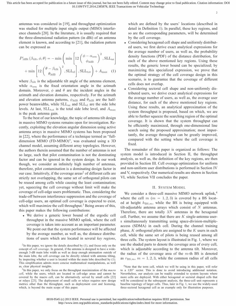
Abstract—We investigate the cell coverage optimization prob-lem for the massive multiple-input multiple-output (MIMO)uplink. By deploying tilt-adjustable antenna arrays at the basestations, cell coverage optimization can become a promisingtechnique which is able to strike a compromise between cov-ering cell-edge users and pilot contamination suppression. Weformulate a detailed description of this optimization problemby maximizing the cell throughput, which is shown to be

mainly determined by the user distribution within several keygeometrical regions. Then, the formulated problem is applied todifferent example scenarios: for a network with hexagonal shapedcells and uniformly distributed users, we derive an analyticallower bound of the ergodic throughput in the objective cell,based on which, it is shown that the optimal choice for the cellcoverage should ensure that the coverage of different cells doesnot overlap; for a more generic network with sectoral shaped cellsand non-uniformly distributed users, we propose an analyticalapproximation of the ergodic throughput. After that, a practicalcoverage optimization algorithm is proposed, where the optimalsolution can be easily obtained through a simple one-dimensionalline searching within a confined searching region. Our numericalresults show that the proposed coverage optimization methodis able to greatly increase the system throughput in macrocellsfor the massive MIMO uplink transmission, compared with thetraditional schemes where the cell coverage is fixed.

Index Terms—Cell coverage, massive MIMO, pilot contamina-tion, uplink.

I. INTRODUCTION

Massive multiple-input multiple-output (MIMO) systems

(a.k.a. large-scale MIMO) have drawn considerable attention

in the literature recently [1]. With a large amount of antennas

Manuscript received December 26, 2013; revised July 1 and October 25,2014. The editor coordinating the review of this paper and approving it forpublication was Y. Gong.S. Jin and X. Gao are with the National Communications Research Lab-

oratory, Southeast University, Nanjing 210096, P. R. China. Emails: {jinshi,xqgao}@seu.edu.cn.J. Wang and Q. Sun are with the School of Electronic and Information

Engineering, Nantong University, Nantong 226019, China. Emails: {wangjue,sunqiang}@ntu.edu.cn. J. Wang is also with Singapore University of Tech-nology and Design, Singapore 138682.M. Matthaiou is with the School of Electronics, Electrical Engineering and

Computer Science, Queen’s University Belfast, Belfast, BT3 9DT, U.K., andwith the Department of Signals and Systems, Chalmers University of Tech-nology, SE-412 96, Gothenburg, Sweden. Email: [email protected] work was supported by National Natural Science Foundation of

China under Grants (61401240, 61222102, 61320106003), the Natural ScienceFoundation of Jiangsu Province under Grant BK2012021, the National Scienceand Technology Major Project of China under Grant 2013ZX03001032-004,the Program for Jiangsu Innovation Team, and the International Science andTechnology Cooperation Program of China under Grant 2014DFT10300.The work of M. Matthaiou has been supported in part by the Swedish

Governmental Agency for Innovation Systems (VINNOVA) within the VINNExcellence Center Chase.

deployed at the base station (BS), it is possible to achieve very

high spectral, as well as, power efficiency with simple linear

transceivers [2], [3], e.g., maximum ratio transmission (MRT)

and maximum ratio combining (MRC). These attractive fea-

tures make massive MIMO a promising technique for the next

generation of mobile communication systems [4].

According to the law of large numbers for independent and

identically distributed (i.i.d.) Rayleigh fading conditions, the

impact of uncorrelated noise and intra-cell interference can

be completely averaged out with massive MIMO, while the

system performance is mainly limited by pilot contamination

caused by pilot reuse in adjacent cells [5]. Considering massive

MIMO systems working in the time division duplex (TDD)

mode,1 orthogonal pilots are sent from users during the

training phase in the uplink, while the BSs perform channel

estimation and use the obtained channel state information

(CSI) for both uplink reception and downlink transmission.

The number of available orthogonal pilots is limited by the

length of the channel coherence time. As the number of

cells and number of users per cell increase, pilot reuse is

inevitable; thus, the uplink channel estimation in one cell will

be contaminated by the uplink channels of users from other

cells that are using the same pilot sequence. To overcome this

intimately negative effect, several works have been document-

ed. Coordinated channel estimation was proposed in [7], while

pilot length reducing techniques were discussed in [8]. On the

other hand, the issue of pilot reuse and allocating mechanism

design was studied in [7], [9], and precoding was investigated

in conjunction with pilot contamination in [5], [10].

Different from the above mentioned approaches, we prefig-

ure that pilot contamination can be, alternatively, suppressed

from a macroscopic perspective, e.g., the cell coverage. In

general, cell coverage adjustment can be realized in practice

via antenna tilting techniques. An early contribution on the

topic of antenna tilting can be found in [11], which was

later extended to universal mobile telecommunications systems

(UMTS) [12], long term evolution (LTE) systems [13], [14]

and network MIMO systems [15]. The topic of antenna tilt

design has been widely studied in recent years [14]–[20],

among which self-optimization of tilt angle was investigated

in [16]–[18], angle signal strength prediction for downtilted

1Note that the tremendous CSI feedback overhead makes the frequencydivision duplex (FDD) mode challenging in massive MIMO systems; for thisreason, most relative works on massive MIMO focus on the TDD mode.It should be highlighted that some novel methods have been proposed toimplement massive MIMO transmission in the FDD mode, e.g., see [6] and thereferences therein. However, a detailed comparison of these different duplexmodes is beyond the main scope of this paper.



2

antennas was considered in [19], and throughput optimization

was studied for multiple input single output (MISO) interfer-

ence channels [20]. In the literature, it is usually required that

the three-dimensional radiation pattern (in dBi) of an antenna

element is known, and according to [21], the radiation pattern

can be expressed as

P |dBi (βtilt, φ, θ) = −min

(

min

[

12

(

φ− αorn

φ3dB

)2

, SLLaz

]

+min

[

12

(

θ − βtilt

θ3dB

)2

, SLLel

]

, SLLtot

)

+Amax (1)

where βtilt is the adjustable tilt angle of the antenna element,

while αorn is the fixed orientation angle in the azimuth

domain. Moreover, φ and θ are the incident angles in the

azimuth and elevation domains, respectively. For the azimuth

and elevation antenna patterns, φ3dB and θ3dB are the half-

power beamwidths, while SLLaz and SLLel are the side lobe

levels. At last, SLLtot is the total side lobe level, and Amax

is the peak antenna gain.

To the best of our knowledge, the topic of antenna tilt design

in massive MIMO systems remains open for investigation. Re-

cently, exploiting the elevation angular dimension using active

antenna arrays in massive MIMO systems has been proposed

in [22], where the performance of a technique termed as “full-

dimension MIMO (FD-MIMO)”, was evaluated using a 3D

channel model, assuming different array topologies. However,

the authors therein assumed that the number of antennas is not

so large, such that pilot contamination is not the dominating

factor and can be ignored in the system design. In our work

though, we consider an infinitely high number of antennas,

therefore, pilot contamination is a dominating design factor in

our case. Intuitively, if the coverage areas2 of different cells are

strictly not overlapping, the same set of orthogonal pilots can

be reused among cells while causing the least contamination;

yet, squeezing the cell coverage without limit will make the

coverage of cell-edge users problematic. Thus, considering the

trade-off between interference suppression and the coverage of

cell-edge users, an optimal cell coverage is expected to exist,

which will maximize the cell throughput.3 Being aware of this,

this paper makes the following contributions:

• We derive a generic lower bound of the ergodic cell

throughput in the massive MIMO uplink, where the cell

coverage is taken into account as an important parameter.

We point out that the system performance will be affected

by the average number, as well as, the distance distribu-

tions of users which are located in several key regions,

2In this paper, we ignore the details described by (1), and focus only on theconcept of cell coverage. In general, if the antenna is designed to have a wide-enough 3-dB main lobe width as well as deep enough attenuation outside ofthe main lobe, the cell coverage can be directly related with antenna tilting,by inspecting whether a user is located within the main lobe described by (1).This simplification admits more concise mathematical manipulations, as wellas, clear physical insights.

3In this paper, we only focus on the throughput maximization of the macrocell, while the users, which are located in cell-edge areas and cannot becovered by the macro cell, can be alternatively served by small cells [22]or relays [23]. The deployment of small cells or relays requires new designmetrics other than the throughput, such as deployment cost and licensing,which, is beyond the main scope of this paper.

which are defined by the users’ locations (described in

detail in Definition 1). In parallel, these key regions, and

so are the corresponding parameters, will be determined

by the cell coverage.

• Considering hexagonal cell shape and uniformly distribut-

ed users, we first derive exact analytical expressions for

the average number of users, as well as, the probability

density functions (PDF) of the distance distribution, for

each of the above mentioned key regions. Using these

results, the generic lower bound can be specialized; by

maximizing this specialized expression, we prove that

the optimal strategy of the cell coverage design in this

scenario, is to guarantee that the coverage of different

cells does not overlap.

• Considering sectoral cell shape and non-uniformly dis-

tributed users, we derive exact analytical expressions for

the average number of users, as well as, the average user

distance, for each of the above mentioned key regions.

Using these results, an analytical approximation of the

system throughput is proposed, based on which, we are

able to further squeeze the searching region of the optimal

coverage. It is shown that the system throughput can

be efficiently maximized, through one-dimensional line

search using the proposed approximation; most impor-

tantly, the average throughput can be greatly improved,

compared with the setting where the cell coverage is

fixed.

The remainder of this paper is organized as follows: The

system model is introduced in Section II, the throughput

analysis, as well as, the definition of the key regions, are then

provided in Section III. Cell overage optimization for uniform

and non-uniform user distributions is performed in Section IV

and V, respectively. Our numerical results are shown in Section

VI, while Section VII concludes the paper.

II. SYSTEM MODEL

We consider a three-cell massive MIMO network uplink,4

where the cell m (m = 1, 2, 3) is covered by a BS locat-

ed at height hBS,m, while the BS is being equipped with

tilt-adjustable antenna arrays which consist of N antennas.

Therefore, there are totally 3N antennas in the hexagonal

cell. Further, we assume that there are K single-antenna user-

s simultaneously transmitting using space-division-multiple-

access (SDMA) in each cell. During the channel training

phase, K orthogonal pilots are assigned to the K users in each

cell, while the same set of pilots is being reused among all

three cells. The system layout is illustrated in Fig. 1, where we

use the shaded parts to denote the coverage area of every cell,

which is adjustable according to the antenna tilt. Moreover,

the radius of the coverage area of the m-th BS is denoted

as rBS,m, m = 1, 2, 3, while the common radius of all cells

4Note that the term cell, which we will be using in this paper, will referto a 120◦ sector. This is done to avoid introducing additional notation.Nevertheless, our analysis can be readily extended to system layouts wheremore cells are deployed. With either hexagonal or sectoral shaped cells thatwill be considered in the subsequent analysis, the three-cell unit represents abaseline topology of larger cells. Thus, later in Fig. 1, we use the widely-usedthree-sectoral hexagonal cell as an example only for illustration purposes.



3

r

r

N

N

N

r

r

Fig. 1: Layout of a three-cell massive MIMO system.

(which, in this figure, is defined as the distance between the

center and the vertex of the hexagon) is denoted as r.

Now, we model the N × 1-sized uplink channel between

the BS in cell m, and user k in cell l (l ∈ {1, 2, 3}) as

hmlk =

√

Pmlk (β

mtilt, φ

mlk , θ

mlk)γ

mlkg

mlk (2)

where gmlk ∼ CN (0N×1, IN×N ) is the i.i.d. fast fading part of

the channel, βmtilt is the tilt angle of BS m, which determines

the corresponding coverage, while φmlk and θmlk are the incident

angles of user k in cell l seen by BS m, in the azimuth and

elevation domains, respectively. Moreover, Pmlk (β

mtilt, φ

mlk , θ

mlk)

is the coefficient of antenna gains, which can be calculated via

(1), and γmlk is the corresponding large-scale fading coefficient

caused by path loss, written as

γmlk =

CPL

(dmlk)α

(3)

where dmlk is the distance between the k-th user in cell l and

the BS in cell m, while α is the path loss coefficient, and CPL

is a constant value determined by the path loss model that is

used.

According to [2, Eq. (13)], as N → ∞, the asymptotic

uplink signal-to-interference ratio (SIR) of user k in cell m

can be written as

SIRuplinkmk =

Pmmk(β

mtilt, φ

mmk, θ

mmk)γ

mmk

∑

l 6=m Pmlk (β

mtilt, φ

mlk , θ

mlk)γ

mlk

(4)

where the denominator corresponds to the inter-cell interfer-

ence caused by pilot contamination, assuming the k-th user

in cell m and l share the same pilot sequence. Moreover, for

the sake of simplicity, we do not consider any power control

scheme in (4) and the transmit power from all users is assumed

to be the same. The sum-throughput (in bps/Hz) of all three

cells is then written as

Ruplinksum =

3∑

m=1

K∑

k=1

log2

(

1 + SIRuplinkmk

)

. (5)

Note that since a pilot allocation strategy is not considered

in this paper, a common term regarding the pilot overhead,

namelyT−Tpilot

T , where T is the block length and Tpilot is the

training length, is omitted in (5) and henceforth for brevity.

Note that the cell coverage optimization should be imple-

mented in a long term basis which implies that the objective

function, i.e. the sum-throughput defined in (5), should be

averaged over all possible user locations. On the other hand,

the coverage of different cells can be optimized separately for

uplink transmission, since the BSs act as receivers, thereby

causing no interference to each other in this scenario; as such,

we can simply focus on the average throughput of only one

cell (denoted as cell m hereafter, without loss of generality),

and the optimization problem can be described as

maxE

[

K∑

k=1

log2

(

1 + SIRuplinkmk

)

]

s.t. rmin ≤ rBS,m ≤ rmax

(6)

where rmin and rmax are respectively the minimum and

maximum coverage of one BS.

Assumption 1: The following assumptions are made to sim-

plify the analysis. Note that the assumptions stated herein ap-

ply only to some special scenarios in our subsequent analysis.

Unless otherwise specified, in the following sections, results

without making these assumptions are still generic and can be

applied to practical scenarios.

1) We assume that the BS hight hBS,m is small compared

with the cell radius. As such, the distance from the k-th

user in cell l to BS m, i.e., dmlk , is calculated using only

the coordinates in the horizontal plane, while hBS,m is

ignored in the calculation.5

2) Similar to [27, Example 2], here we assume, for the

sake of simplicity, that the tilt-adjustable antenna array

has uniform gain over the span of its main lobe, i.e., for

the users satisfying that dmlk ≤ rBS,m, we let

Pmlk (β

mtilt, φ

mlk , θ

mlk) = 1. (7)

On the other hand, for the users located outside of the

3-dB main lobe, according to (1), the antenna gain is

constant and can be written as

Pmlk (β

mtilt, φ

mlk, θ

mlk) = −SLLtot +Amax , C. (8)

3) Since the value of CPL in (3) will not affect the analysis,

hereafter we simply set CPL = 1 for the ease of

description.

III. THROUGHPUT ANALYSIS

In this section, we analyze the ergodic throughput in cell

m, i.e., the objective in (6), aiming at representing it in terms

of the user location distributions. This will be the basis of our

subsequent coverage analysis. To proceed, we first introduce

the following definition:

5As will be shown later, cell coverage optimization demonstrates highsuperiority mainly in the scenarios where most users are located in the cell-edge region. As such, considering a typical cell configuration where the heightof the BS is approximately 30m, while the cell radius is 500m, the error causedby this simplification will be small enough to be ignored.



4

BS m BS l

m

mA

m

mA

m

lA

m

lA

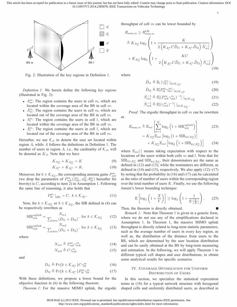
Fig. 2: Illustration of the key regions in Definition 1.

Definition 1: We herein define the following key regions

(illustrated in Fig. 2):

• Amm: The region contains the users in cell m, which are

located within the coverage area of the BS in cell m.

• Amm: The region contains the users in cell m, which are

located out of the coverage area of the BS in cell m.

• Aml : The region contains the users in cell l, which are

located within the coverage area of the BS in cell m.

• Aml : The region contains the users in cell l, which are

located out of the coverage area of the BS in cell m.

Hereafter, we use KA to denote the user set located within

region A, while A follows the definitions in Definition 1. The

number of users in region A, i.e., the cardinality of KA, will

be denoted as KA. Note that we have

KAmm+KAm

m= K (9)

KAml+KAm

l= K. (10)

Moreover, for k ∈ KAmm, the corresponding antenna gains Pm

mk

(we drop the parameters of Pmmk(β

mtilt, φ

mlk, θ

mlk ) hereafter for

brevity) is C, according to item 2) in Assumption 1. Following

the same line of reasoning, it also holds that

Pmlk |dBi = C, k ∈ KAm

l. (11)

Now, for k ∈ KAmmor k ∈ KAm

m, the SIR defined in (4) can

be respectively rewritten as

SIRuplinkmk =

Nm1∑

l 6=m (Dl1 +Dl2), for k ∈ KAm

m(12)

SIRuplinkmk =

Nm2∑

l 6=m (Dl1 +Dl2), for k ∈ KAm

m(13)

where

Nm1 , Pmmkγ

mmk (14)

Nm2 , Cγmmk (15)

and

Dl1 , Pr{k ∈ KAml}Cγm

lk (16)

Dl2 , Pr{k ∈ KAml}Pm

lk γmlk . (17)

With these definitions, we propose a lower bound for the

objective function in (6) in the following theorem:

Theorem 1: For the massive MIMO uplink, the ergodic

throughput of cell m can be lower bounded by

Rsum,m ≥ RLBsum,m

, KAmmlog2

1 +K

2(

KAmlCDl1 +KAm

lDl2

)

N−1m1

+KAmmlog2

1 +KC

2(

KAmlCDl1 +KAm

lDl2

)

N−1m2

(18)

where

Dl1 , El [γmlk ] |k∈KAm

l

(19)

Dl2 , E[Pmlk γ

mlk ] |k∈KAm

l

(20)

N−1m1 , E[(Pm

mkγmmk)

−1] |k∈KAmm

(21)

N−1m2 , E[(γm

mk)−1] |k∈KAm

m

. (22)

Proof: The ergodic throughput in cell m can be rewritten

as

Rsum,m , Eml

[

K∑

k=1

log2

(

1 + SIRuplinkmk

)

]

(23)

= KAmmEml

[

log2(

1 + SIRk∈Amm

)]

+KAmmEml

[

log2

(

1 + SIRk∈Amm

)]

(24)

where Eml[·] means taking expectation with respect to the

locations of the users within both cells m and l. Note that for

SIRk∈Ammand SIRk∈Am

m, their denominators are the same as

defined in (12) and (13), while the nominators are different, as

defined in (14) and (15), respectively. We also apply (12)–(17)

by noting that the probability in (16) and (17) can be calculated

as the ratio of number of users within the corresponding region

over the total number of usersK . Finally, we use the following

Jensen’s lower bounding technique:

E

[

log2

(

1 +X

Y

)]

≥ log2

(

1 +1

E[

YX

]

)

. (25)

Then, the theorem is directly obtained.

Remark 1: Note that Theorem 1 is given in a generic form,

where we do not use any of the simplifications declared in

Assumption 1. In Theorem 1, the massive MIMO uplink

throughput is directly related to long-term statistic parameters,

such as the average number of users in every key region, as

well as, the distribution of the distance from users to the

BS, which are determined by the user location distribution

and can be easily obtained at the BS by long-term measuring

and estimation. In the following, we will apply Theorem 1 to

different typical cell shapes and user distributions, to obtain

some analytical results for specific scenarios.

IV. COVERAGE OPTIMIZATION FOR UNIFORM

DISTRIBUTION OF USERS

In this section, we specialize the statistical expectation

terms in (18) for a typical network structure with hexagonal

shaped cells and uniformly distributed users, as described in



5

Assumption 2. After that, the optimal rBS,m is found for this

scenario.

Assumption 2 (Uniform Distribution of Users): The shape

of the cells and the user locations satisfy

1) The cells are assumed to be hexagonal shaped.

2) All users are assumed to be uniformly distributed in their

corresponding cells.

As such, due to the symmetry of this system layout, the

optimal coverage areas (i.e., rBS,m,m = 1, 2, 3) of all threeBSs will be the same. Thus, hereafter in this section, we drop

the subscript m in rBS,m, and simply use rBS to denote the

parameter to be optimized.

A. Parameter Specification for Throughput Analysis

We first specialize the parameters that are needed in cal-

culating (18), in the scenario described by Assumption 2. At

first, we evaluate the average number, as well as, the PDF of

their distances to BS m, of the users distributed in every key

region defined in Definition 1. The results proposed in this

subsection will serve as a necessary basis of the subsequent

rate analysis.

Proposition 1: With Assumption 2, the average number of

users located in every key region defined in Definition 1 can

be respectively evaluated as (26) and (27) at the bottom of this

page, and

KAmm= K −KAm

m(28)

KAml= K −KAm

l. (29)

Proof: Under the assumption that the users are uniformly

distributed in the cells, the number of users in a region A is

proportional to the area of A, thus it can be obtained as

KA = min

(

K,KA(A)Acell

)

(30)

where A(·) is the area of a region, while Acell is the area of

each rhombus cell, which is

Acell =

√3r2cell2

. (31)

Using (30) and (31), (26) and (27) are obtained using simple

but tedious geometrical manipulation methods, while (28) and

(29) are obtained by (9) and (10).

Proposition 1 provides exact analytical expressions for the

average number of uniformly distributed users, for each of

the key regions defined in Definition 1. Then, regarding the

distributions of dmlk and dmmk, the following two lemmas are

respectively derived:

Lemma 1: The PDF of the random distance between the

vertex of one rhombus and a uniformly distributed node in

an adjacent rhombus, sharing the same side but being with

different orientation, is written as

fdmlk(x) =

0, x <√32 r

4x√3r2

arccos√3r

2x ,√32 r ≤ x ≤ r

πx√3r2− 2x√

3r2arccos

√3r

2x , r < x ≤√3r

πx3√3r2− 2x√

3r2arccos

√3rx ,

√3r < x ≤ 2r

0, x > 2r.(32)

Proof: We use the area-ratio approach used in [25],

where the CDF of the distance between one fixed point and

a uniformly distributed point in a cell, can be written in the

form of the ratio of two corresponding areas. The area of the

rhombus cell was determined in (31). On the other hand, the

area of Aml can be determined separately as in (33) at the

bottom of this page. Thus, the CDF of dmlk can be obtained by

noting thatA(Am

l )Acell

, as described in (34) (See bottom of the next

page), and the corresponding PDF is derived by differentiating

(34) with respect to x.

Lemma 2: The PDF of the random distance between a

uniformly distributed node in a rhombus and its vertex, is

KAmm=

K2πr2BS

3√3r2

, rBS ≤√32 r

2K2(

π6−arccos

√3r

2rBS

)

r2BS+r√3√

r2BS− 3

4r2

√3r2

,√32 r < rBS ≤ r

K, rBS > r

(26)

KAml=

0, rBS ≤√32 r

K2r2BS arccos

√3r

2rBS−r√3√

r2BS− 3

4r2

√3r2

,√32 r < rBS ≤ r

K

(√r2BS− 3

4r2− r

2

)√3

2r+

(

π2−arccos

√3r

2rBS

)

r2BS−√

32

r2

√3r2

, r < rBS ≤√3r

K

(

π6−arccos

(√3r

rBS

))

r2BS+√3r√

r2BS−3r2

√3r2

,√3r < rBS ≤ 2r

K, rBS > 2r

(27)

A (Aml ) =

d2 arccos√3r2d −

√

d2 − 34r

2√3r2 ,

√3r2 ≤ d ≤ r

πd2

4 − πr2

6 − d2

2 arccos√3r2d +

√3r4

(√

d2 − 34r

2 − r2

)

, r < d ≤√3r

112π

(

d2 − 3r2)

− d2

2 arccos√3rd +

√3r2

√d2 − 3r2,

√3r < d ≤ 2r.

(33)



6

written as

fdmmk

(x) =

4πx3√3r2

, x <√3r2

4π3√3r2

x− 8√3r2

x arccos√3r

2x ,√3r2 ≤ x ≤ r

0, x > r.(35)

Proof: The proof follows the same line of reasoning as

that in the proof of Lemma 1.

Having the results in Proposition 1, Lemma 1 and Lemma 2

in hand, we are now ready to proceed with deriving analytical

expressions for the expectation terms (19)–(22). These results

are provided in the following proposition:

Proposition 2: In the typical scenario under Assumption 1

and Assumption 2, the expectation terms (19)–(22) can be

analytically evaluated as (36) and (37) at the bottom of this

page, where Gi(x), i = 1, 2, 3 are respectively defined as

G1(x) , C1(α, r)x2−α

− 2

∞∑

n=0

1

4nC2(α, n, r)x

−α−2n+1 (38)

G2(x) ,∞∑

n=0

1

4nC2(α, n, r)x

−α−2n+1 (39)

G3(x) , −C1(α, r)

3x2−α + 2

∞∑

n=0

C2(α, n, r)x−α−2n+1

(40)

where

C1(α, r) ,1

2− α

2π√3r2

(41)

C2(α, n, r) ,

(

2nn

)

3nr2n−1

4n (2n+ 1) (−α− 2n+ 1). (42)

On the other hand, N−1m1 and N−1

m2 are respectively written as

N−1m1 =

Acell

A (Amm)

×

H1(x)∣

∣rBSrmin

, rBS <√3r2

H1(x)∣

∣

∣

√3r/2

rmin +H2(x)∣

∣

∣

rBS√3r/2

,√3r2 ≤ rBS ≤ r

H1(x)∣

∣

∣

√3r/2

rmin +H2(x)∣

∣

∣

r√3r/2

, x > r

(43)

N−1m2 =

Acell

A(

Amm

)

×

H1(x)∣

∣

∣

√3r/2

rBS +H2(x)∣

∣

∣

r√3r/2

, rBS <√3r2

H2(x)∣

∣rrBS

,√3r2 ≤ rBS ≤ r

0, x > r

(44)

where H1(x) and H2(x) are defined as

H1(x) ,2

3C1(−α, r)x2+α (45)

H2(x) ,−43

C1(−α, r)x2+α

+

∞∑

n=0

1

4n−1C2(−α, n, r)x−2n+α+1. (46)

Proof: See Appendix I.

The parameters derived in Proposition 2 are in a complicated

form, and so is the corresponding throughput lower bound in

Theorem 1; however, the bound expression consists of only

elementary functions. Thus, it will be convenient to calculate

numerically in practice in a far more efficient manner com-

Fdmlk(x) =

0, x <√32 r

2x2

√3r2

arccos√3r

2x − 1r

√

x2 − 34r

2,√32 r ≤ x ≤ r

πx2

2√3r2− π

3√3− x2

√3r2

arccos√3r

2x + 12r

(√

x2 − 34r

2 − r2

)

+A(Am

l )|rBS=r

Acell, r < x ≤

√3r

π(x2−3r2)6√3r2

− x2

√3r2

arccos√3rx + 1

r

√x2 − 3r2 +

A(Aml )

∣

∣

∣rBS=√

3r

Acell,

√3r < x ≤ 2r

1, x > 2r

(34)

Dl1 =Acell

A(

Aml

) ×

G1(x)∣

∣

∣

r√3r/2

+G2(x)∣

∣

∣

√3r

r +G3(x)∣

∣

∣

2r√3r

, rBS <√32 r

G1(x)∣

∣rrBS

+G2(x)∣

∣

∣

√3r

r +G3(x)∣

∣

∣

2r√3r

,√32 r ≤ rBS ≤ r

G2(x)∣

∣

∣

√3r

rBS+G3(x)

∣

∣

∣

2r√3r

, r < rBS ≤√3r

G3(x)∣

∣2rrBS

,√3r < rBS ≤ 2r

0, rBS > 2r

(36)

Dl2 =Acell

A (Aml )×

0, rBS <√32 r

G1(x)∣

∣

∣

rBS√3/2r

,√32 r ≤ rBS ≤ r

G1(x)∣

∣

∣

r√3r/2

+G2(x) |rBSr , r < rBS ≤

√3r

G1(x)∣

∣

∣

r√3r/2

+G2(x)∣

∣

∣

√3r

r +G3(x)∣

∣

∣

rBS√3r

,√3r < rBS ≤ 2r

G1(x)∣

∣

∣

r√3r/2

+G2(x)∣

∣

∣

√3r

r +G3(x)∣

∣

∣

2r√3r

, rBS > 2r

(37)



7

pared to time-consuming Monte-Carlo simulations. Numerical

results, which we will show later, demonstrate that this lower

bound is capable of capturing the exact changing trend of

the ergodic sum rate versus rBS. As such, it is useful in the

subsequent coverage optimization analysis.

B. Coverage Optimization

Based on Theorem 1 and Proposition 2, we obtain the

following corollary on the coverage optimization in the con-

sidered network with uniform distribution of users:

Corollary 1: With the parameters derived in Proposition 2,

the optimal rBS that maximizes the ergodic throughput lower

bound proposed in Theorem 1, is written as

ropt

BS =

√3r

2. (47)

Proof: See Appendix II.

Corollary 1 indicates that for the considered network layout

with Assumption 1 and Assumption 2, where the positions

of all users are uniformly distributed in hexagonal shaped

cells, the benefit gained from enlarging the coverage area of

the BS (which means that more edge users will be covered),

will be less than the rate loss caused by pilot contamination,

which also stems from the coverage area enlargement. Thus,

one guideline for cell planning in massive MIMO systems in

this scenario, will be that the coverage areas of different cells

should not overlap with each other.

Note that the scenario considered in this section, is a

simplified ideal model which is not applicable for practical

designs. Nevertheless, using this model, we can theoretically

showcase the fundamental tradeoff between serving cell-edge

users and pilot contamination suppression. For more practical

scenarios with non-unit antenna gains and non-uniform user

distributions, it can be anticipated that ropt

BS may be shifted

from√3r2 . In the following, we will show for more generic

networks, where the users are non-uniformly distributed, that

coverage optimization will bring significant throughput gains.

V. COVERAGE OPTIMIZATION FOR NON-UNIFORM

DISTRIBUTION OF USERS

It is not surprising that uniform user distribution leads to the

conclusion that non-overlapping coverage should be optimal.

However, when the users are not uniformly distributed, the

optimal coverage should be carefully re-calculated. In this

section, we extend the analysis to more general networks with

non-uniform user distribution. For the ease of description of

this scenario, we also change the cell-shape assumption to be

sectoral shaped, which, is also typical and widely adopted in

the corresponding literature [26]. The scenario considered in

this section is summarized in the following assumption:

Assumption 3 (Non-Uniform Distribution of Users): The

cell shape and the user locations distribution are respectively

determined as:

1) The cells are assumed to be sectoral shaped.

2) The users are non-uniformly distributed in each cell; al-

so, the user locations’s distributions are different among

all three cells. This will be described by different number

cell l cell m

BS m BS l

N N

( ) 3 1 r−r

inner-cell region

cell-edge region

Fig. 3: Illustration of the inner-cell and cell-edge regions.

of inner-cell and cell-edge users, as introduced in the

following.

3) For the ease of analysis, we further divide a cell into two

areas (described in Fig. 3): the inner-cell area (where

d < (√3 − 1)r) and the cell-edge area (where (

√3 −

1)r < d < r). For cell m, the number of users in these

two areas are denoted asK innerm andKedge

m , respectively.

As such, we have

K = K innerm +Kedge

m . (48)

Moreover, we assume that the users are uniformly dis-

tributed in these two areas, respectively.

It is noted that with Assumption 3.3), overlapping occurs

only among the cell-edge regions in different cells, while

overlapping will not happen for the inner-cell regions. Thus,

this definition of cell-edge and inner-cell areas is meaningful

and sufficiently realistic in practice.

A. Parameter Specification for Throughput Analysis

Following the same methodology as in Section IV, we first

derive exact analytical expressions for the average number of

users, as well as, the average distance to BS m, for the users

distributed in the key regions defined in Definition 1. These

results serve as necessary basis for the following rate analysis.

Proposition 3: With Assumption 3, the average number of

users located in every key region defined in Definition 1 can

be respectively evaluated as

KAmm= K inner

m +Kedgem

α2m − (

√3− 1)2

1− (√3− 1)2

(49)

KAml= K

edgel

3

π

1

1−(√

3− 1)2

(

α2m arccos

α2m + 2

2√3αm

(50)

− α2m + 2

12

√

12α2m − (α2

m + 2)2

+ arccos4− α2

m

2√3− 4− α2

m

12

√

12− (4− α2m)

2

)

(51)

where we define αm ,rBS,m

r for brevity. Moreover, we have

KAmm= K −KAm

m(52)

KAml= K −KAm

l. (53)

Proof: Denoting the area of the inner-cell region as

Ainner, and the area of the cell-edge region as Aedge, we can



8

respectively evaluate them as

Ainner =π(√

3− 1)2

3r2 (54)

Aedge =π

3

(

1−(√

3− 1)2

)

r2. (55)

On the other hand, using simple geometry, we can get

A(Amm) =

πα2mr2

3(56)

A(Aml ) (57)

= r2(

α2m arccos

α2m + 2

2√3αm

− α2m + 2

12

√

12α2m − (α2

m + 2)2

+ arccos4− α2

m

2√3− 4− α2

m

12

√

12− (4− α2m)2

)

(58)

Then, the number of users in each region can be respectively

calculated as

KAmm= K inner

m +Kedgem

A (Amm)−Ainner

Aedge(59)

KAml= K

edgel

A (Aml )

Aedge. (60)

Following the same line of reasoning as that used in proving

Proposition 1, and using simple geometry, the proposition can

be proved.

In the following proposition, we derive the average distance

from the users distributed in every key region to BS m.

Proposition 4: With Assumption 3, and for the users dis-

tributed in every key region defined in Definition 1, their

average distance to BS m can be respectively evaluated as

dmm =Kinner

KAmm

2

3

(√3− 1

)

r

+

(

1− Kinner

KAmm

)

2

3

α3m − (

√3− 1)3

α2m − (

√3− 1)2

r (61)

dmm =2

3

1− α3m

1− α2m

r (62)

where dmm , E [dmmk] for all k ∈ KAmm, is the average distance

from the users located in region Amm to BS m, while dmm,

dml and dml are similarly defined. For the two terms dml and

dml , their expressions become extremely complicated in this

generic scenario, thus are omitted here; nevertheless, we will

give a brief description on the corresponding calculation of

these two terms, in the proof of this proposition.

Proof: See Appendix III.

The results from Proposition 3 and Proposition 4 are now

directly applied to the rate analysis. Note that the assumption

of non-uniform distribution of users makes the optimization

of rBS,m much more complicated than that in the uniformly-

distributed scenario. For this reason, instead of using the lower

bounding technique in Theorem 1, we hereafter make use of

an approximation of Rsum,m, which is given in the following

proposition:

Proposition 5: For the massive MIMO uplink, the ergodic

sum rate of the users in cell m can be approximated by (63)

at the bottom of this page, where the average number of

users KAmm, KAm

m, KAm

land KAm

lare defined in Proposition

3, while the average distances dmm, dmm, d

ml and dml can be

obtained via Proposition 4.

Proof: The proposition is obtained by simply replacing

the random distance terms in the SIR term in (24), with their

statistical expectations.

It is noted that (63) is a generic result, which is not restricted

to particular cell shapes.6 Further applying Proposition 2 and

Proposition 3 to (63), the derived result still consists of only

elementary functions, thus can be conveniently calculated in

practice. Most importantly, our numerical results in Section VI

will show that using the rate approximation in Proposition 5

for cell optimization can provide significant throughput gains.

B. Coverage Optimization

The rate approximation proposed in Proposition 5 is still too

complicated for the derivation of the exact optimal solution

of rBS,m. However, as aforementioned, it consists of only ele-

mentary functions, thus the optimal rBS,m can be conveniently

obtained through one-dimensional line searching. Moreover,

with the help of (63), the searching range of the optimal rBS,m

can be further squeezed, thereby making the implementation

of cell coverage optimization more feasible in practice. As a

starting point and, without loss of generality, we can make the

following generic assumption that dmlk is distributed in a range

bounded as:7

dml,min ≤ dmlk ≤ dml,max. (64)

Similarly, for dmmk we assume

0 ≤ dmmk ≤ dmm,max. (65)

6The parameters in (63) can be calculated with Assumption 3. However,(63) itself is generic.

7The assumption that minl,l 6=m

dml,min

< dmm,max is reasonable in practice.

For example, in the network described in Fig. 2, where hexagon shaped cells

are assumed, we have dml,min

=√

3r2

and dmm,max = r; while in Fig. 3,

where sector shaped cells are considered, we have dml,min

= (√3− 1)r and

dmm,max = r.

Rsum,m ≈ Rapproxsum,m

, KAmmlog2

1 +(dmm)−α

∑

l 6=m

(

KAml(dml )

−α+KAm

lC(

dml)−α

)

+KAmmlog2

1 +C(

dmm)−α

∑

l 6=m

(

KAml(dml )

−α+KAm

lC(

dml)−α

)

(63)



9

Algorithm 1 Practical cell coverage optimization

1. Set KA = 0, dA = 0. Set t = 0, Tstat = T0, where

T0 is a predefined time interval for updating the cell

coverage;

2. When a user k gets accessed, letKA = KA+1, dA =dA + dk if k ∈ KA (dk is the distance from user k

to the objective BS);

3. When t = Tstat, calculate the average distance

dA = dA

KA. Then, use Proposition 5 and Corollary

2 to determine the optimal coverage;

4. Compare the values ofKA with that in the prior loop.

If the change is significant (e.g., greater than αth%where αth is a predefined threshold), reduce T0;

similarly, if the change is non-significant, maintain

or enlarge the value of T0 in Step 1 and start the

new loop.

Then, the following corollary can be obtained:

Corollary 2: The optimal rBS,m, which maximizes the er-

godic uplink sum rate approximation (63), will be within the

interval

minl,l 6=m

dml,min ≤ ropt

BS,m ≤ dmm,max. (66)

Proof: From (63), it is clear that when rBS,m >

dmm,max, the terms KAmm, KAm

m, as well as, dmm and dmm

will be fixed. As such, if rBS,m keeps enlarging, the on-

ly term which will be affected in (63) will be the in-

terference term caused by pilot contamination, i.e., D ,∑

l 6=m

(

KAml(dml )

−α+KAm

lC(

dml)−α

)

in the denominator.

As such, Rsum,m will be decreasing with respect to rBS,m. On

the other hand, when rBS,m < minl,l 6=m

dml,min, the interference

term D in (63) will be fixed; as such, it is easy to shown

that Rsum,m will be increasing with respect to rBS,m in this

regime.

As a conclusion of this section, Proposition 5 provides an

effective objective function while Corollary 2 further squeezes

the searching range within which this objective function can

be maximized. With these results in hand, the optimal rBS,m

can be easily found by simple one-dimensional line searching

techniques. Based on Proposition 5 and Corollary 2, we

propose a cell coverage optimization scheme which can be

easily implemented in practice, as described in Algorithm 1.

Our numerical results will show that the proposed scheme

significantly improves the system throughput, compared with

fixed cell coverage.

VI. NUMERICAL RESULTS

As a necessary basis of the subsequent simulations, we first

need to numerically validate the results derived in Lemmas

1, 2, as well as, the results in Propositions 1, 3, and 4. At

first, the CDFs of dmmk and dmlk are shown in Fig. 4, where

the cell radius is set to be r = 500m, and the curves are

respectively obtained by both Monte-Carlo simulations and the

analytical expressions in Lemmas 1 and 2. An exact match

between the Monte-Carlo and the analytical results can be

0 200 400 600 800 10000

0.1

0.2

0.3

0.4

0.5

0.6

0.7

0.8

0.9

1

Cell radius ( r )

Cu

mu

lative

pro

ba

bili

ty cell m cell l

Monte-CarloAnalyt. result

Fig. 4: CDF of dmmk and dmlk in a network with hexagonal

shaped cells and uniformly distributed users.

observed. Recalling the proofs of Lemma 1, Lemma 2 and

Proposition 1, the average numbers of users described in (26)

and (27), can be directly related to the PDFs described in

(32) and (35). As a consequence, Fig. 4 also does prove the

accuracy of Proposition 1.

380 400 420 440 460 480 5000

10

20

30

40

50

60

70

80

90

100

rBS,m

(m)

Nu

mb

er

of

use

rs

Am

m

Al

m

Monte-CarloAnalyt. result

Fig. 5: The average number of users vs. rBS,m in a network

with sectoral shaped cells and non-uniformly distributed users.

Then, we validate Proposition 4 by depicting the average

number of users in regions Amm and Am

l , versus the value of

rBS,m in Fig. 5. We set r = 500m and K = 100 in the

simulation. Again, a perfect match between the Monte-Carlo

and analytical results is shown. Moreover, as rBS,m increases,

the average numbers of users in regions Amm and Am

l are both

increasing, which indicates that while serving more users in

cell m, BS m will face more interference from cell l. As a

consequence, an optimum coverage which is able to strike a

compromise between these contradicting effects does exist, as

will be shown later.

In Fig. 6, we compare the Monte-Carlo result with the lower



10

100 200 300 400 500 600 700 800 900 10000

10

20

30

40

50

60

70

80

90

rBS

(m)

Erg

od

ic t

hro

ug

hp

ut

in c

ell

m (

bp

s/H

z)

Monte-CarloLower boundApprox.

Fig. 6: Ergodic throughput in cell m vs. rBS in a network with

hexagonal shaped cells and uniformly distributed users.

bound (Theorem 1) and the approximation (Proposition 5)

of the ergodic throughput in cell m, vs. the coverage area

of the BSs, i.e., rBS. In the simulation, we set r = 500m,K = 10. Assuming unit power gains within the BS coverage

area and −20dB outside that coverage, the Monte-Carlo result

is calculated directly using the SIR definition in (4), averaged

over 500 times of random generations of the users’ positions.

It is shown that the lower bound, as well as, the approximation

are able to reflect the same changing trend as the Monte-

Carlo result, thus are qualified to be used in the coverage

optimization design. Note that the tightness of the lower bound

is different at different values of rBS; this is because the

bounding technique in (25) has been respectively applied to

two weighted terms as shown in (24); with different value

of rBS, the weight of these two terms, namely KAmm

and

KAmm, will be different, thus leading to different tightness of

the combined lower bound. Nevertheless, it is shown that all

curves achieve their maximum at the same value of rBS, which

is about 433m as shown in the figure. This result, which is in

fact√32 r, coincides perfectly with our analysis and the results

drawn in Corollary 1.

In Fig. 7, the achievable uplink throughput in cell m is

depicted versus αinnerl , where

αinnerl ,

K innerl

K(67)

is the parameter indicating the user distribution in cell l.

When αinnerl = 1, it means that all users in cell l are

located in the inner-cell regions, thereby causing the least

pilot contamination to the users in cell m; on the other hand,

when αinnerl = 0, all users in cell l are located in the cell-

edge region, and the system performance will be severely

degraded by pilot contamination. In the simulation, we as-

sume that the users in cell m are uniformly distributed, i.e.,

αinnerm = Ainner

Acell. In the figure, different results are shown when

the cell coverage is fixed to be rBS,m = r, for m = 1, 2, 3,as well as, the setting where the cell coverage is adjustable

0 0.2 0.4 0.6 0.8 10

50

100

150

200

250

300

350

αinner

l

Ave

rag

e t

hro

ug

hp

ut

in c

ell

m (

bp

s/H

z) r

BS,m = r

Monte-CarloApprox.

Fig. 7: Throughput in cell m vs. αinnerl in a network with

sectoral shaped cells and non-uniformly distributed users.

according to the changing of the user distributions, i.e., αinnerl .

Moreover, for the coverage-adjustable setting, we compare the

Monte-Carlo result (where the searching is carried out directly

using (23)) and the one-dimensional line searching using the

approximation proposed in Proposition 5. It is shown that (63)

in Proposition 5 is a very effective metric, which leads to

nearly the same global optimum achieved by tedious Monte-

Carlo simulation. Most importantly, the graph demonstrates

that coverage optimization results in significant gains in the

system throughput, compared with the conventional setting

where the coverage is fixed. Specifically, when the value of

αinnerl is small, i.e., more interfering users are located in the

cell-edge regions of the adjacent cells, the gains brought by

cell coverage optimization become substantial. As anticipated,

when αinnerl grows large, the benefits of coverage optimization

are decreasing, since pilot contamination vanishes.

We now show the optimal cell coverage for different user

distribution conditions, determined by both αinnerm and αinner

l

in Fig. 8. The results indicate that when the number of

cell-edge users increases in adjacent cells, i.e., when αinnerl

decreases, the optimal coverage of cell m should be reduced.

On the other hand, with increasing αinnerm , i.e., more inner-

cell users in cell m, the optimal coverage of cell m also

decreases. Note that the optimal coverage is always less

than r = 500m, which confirms our conclusion drawn from

Corollary 2. Essentially, it indicates that if the throughput is

maximized for the macro cells, the cell-edge users, which are

located in the center region of the three-cell unit shown in

Fig. 3, will not be covered by any of these cells. As such,

small cell stations are necessary to be placed in this area to

provide seamless coverage of the entire network.

At last, we apply the cell coverage optimization Algorithm

1 to a practical network, where a typical 19-cell network is

considered, as shown in Fig. 9. In the figure, we use black

dots to denote the positions of the BSs, each consisting of

three 120◦ sectoral antenna arrays implemented with large

but finite number of antennas, i.e., from 100 to 500. In



11

00.2

0.40.6

0.81

0

0.5

1350

400

450

500

αinner

mα

inner

l

r BS

,m

opt

Fig. 8: Optimal cell coverage vs. αinnerl and αinner

m in a net-

work with sectoral shaped cells and non-uniformly distributed

users.

−2000 −1000 0 1000 2000 3000−2000

−1500

−1000

−500

0

500

1000

1500

2000

2500

coordinate x

co

ord

ina

te y

Fig. 9: Layout of the 19-cell network with randomly located

users.

every sector, 10 users are non-uniformly located and the usersbelong to different sectors are described respectively using

circle, triangle and x-mark in the figure. The user location

distribution is determined by the number of inner-cell and cell-

edge users as described in Fig. 3, which, are independently

and randomly generated among different sectors as well as

different simulation trials.

In Fig. 10, we evaluate the average throughput of the central

cell among all 19 cells using Monte-Carlo simulation. The

throughput is plotted versus increasing number of antennas.

As a benchmark, a reference coverage determination method

(labeled as “no overlap” in the figure), which simply deter-

mines the coverage of every sector to avoid overlapping, is

100 150 200 250 300 350 400 450 50050

60

70

80

90

100

110

Number of antennas per sector

Ave

rag

e t

hro

ug

hp

ut

pe

r ce

ll (b

ps/H

z)

Algorithm 1

No overlap

Fig. 10: Average throughput per cell vs. number of antennas

per sector.

also illustrated. It is shown that the proposed cell coverage

optimization algorithm significantly increases the throughput.

As anticipated, the throughput increment gets larger as the

number of antenna increases, for the reason that our algorithm

is designed based on the asymptotic rate approximation with

an infinite number of antennas.

As a last comment, we emphasize the impact of number

of antennas on our proposed algorithm. With the assumption

of an infinite number of antennas, interference only comes

from pilot contamination caused by the users who are using

the same pilot in adjacent cells (or sectors). On the other

hand, with finite number of antennas, interference also comes

from 1) the other users in the same cell, and 2) all users in

adjacent cells (assuming a frequency reuse factor 1). Since ouralgorithm is based on the asymptotic assumption, the finite-

antenna interference is ignored in the design. However, we

note that with large but finite number of antennas (such as

100–500 as shown in Fig. 10), the mutual interference betweentwo independent wireless links is anyways very small (albeit

not zero, which, only holds for the extreme case). In this finite

antenna regime, considering only the pilot-contaminating user,

other than all users in adjacent cells, is a reasonable choice

when performing cell coverage optimization. Although the

achievable throughput is much less than that of the infinite-

antenna case, the result in Fig. 10 clearly shows that significant

gains can still be realized by the proposed algorithm with large

but finite number of antennas.

VII. CONCLUSIONS

In this paper, cell coverage optimization was investigated

in the massive MIMO uplink. We first formulated a detailed

description of this important optimization problem, where it

was pointed out that the system throughput will be determined

by the user distributions in some key geometrical regions. The

formulated problem was then applied to different practical

scenarios. For a network with hexagonal shaped cells and

uniformly distributed users, an analytical lower bound of the



12

ergodic sum rate in the objective cell was derived, based

on which it was proved that the optimal choice for the cell

coverage should ensure that the coverage of different cells

does not overlap. For a more generic network with sectoral

shaped cells and non-uniformly distributed users, we proposed

an analytical approximation of the ergodic sum rate; after that,

the optimal solution can be easily obtained through a simple

one-dimensional line searching within a bounded searching

region. Our numerical results showcased that the proposed

coverage optimization method can substantially increase the

system throughput for the massive MIMO uplink transmission,

compared with the traditional scheme where the cell coverage

is fixed.

APPENDIX I

PROOF OF THEOREM 1

Starting with evaluating Dl1, we have

Dl1 =

∫ dAml

,max

dAml

,min

PL(x)fAml(x)dx =

∫ 2r

rBS

1

xαfAm

l(x)dx

(68)

where dAml,min and dAm

l,max are the minimum and maximum

distances between the users in the region Aml and BS m,

respectively; PL(x) is the function of path loss defined in

(3), while

fAml(x) , fdm

lk(x)

∣

∣

∣for k∈KAml

= Pr(

dmlk = x | k ∈ KAml

)

(69)

=Pr

(

dmlk = x, k ∈ KAml

)

Pr(

k ∈ KAml

) =fdm

lk(x)

A(

Aml

)/

Acell

(70)

is the PDF of dmlk conditioned on that the objective user is lo-

cated in the regime Aml . To continue evaluating (68), we make

use of Lemma 1, and introduce the infinite series expansion

of arccos(x) such that arccos(x) = π2 −

∑∞n=0

(2nn )x2n+1

4n(2n+1) , for

the ease of analysis. Then, the indefinite integral of 1xα fAm

l(x)

can be derived as

∫

1

xαfAm

l(x)dx =

0, x <

√3

2r

G1(x),

√3

2r ≤ x ≤ r

G2(x), r < x ≤√3r

G3(x),√3r < x ≤ 2r

0, x > 2r

(71)

where Gi(x), i = 1, 2, 3 were defined in (38)–(40). Then, (36)can be directly obtained by applying (71) to (68). Note that

Dl2 can be obtained on a similar note.

Then, we seek to evaluate Nm1 and Nm2. We first evaluate

the following indefinite integral as

∫

xαfdmm(x)dx =

H1(x), x <

√3r

2

H2(x),

√3r

2≤ x ≤ r

0, x > r

(72)

where H1(x) and H2(x) were defined in (45) and (46). Then,the following proof follows the same line of reasoning as that

used before, which leads us to (43) and (44).

APPENDIX II

PROOF OF COROLLARY 1

First, consider the regime where rBS ≤√3r2 , then (18)

can be simplified as (73) at the bottom of this page, where

C1 = 2C(

G1(x)|r√3r/2 + G2(x)|√3r

r + G3(x)|2r√3r

)

is a

constant which is independent of rBS. Then, we investigate

the monotonicity of (73) by taking the derivative with respect

to rBS. By doing so, it can be shown that in the regime

rBS ≤√3r2 , RLB

sum,m is monotonously increasing. Similarly,

in the regime where rBS >√3r2 , RLB

sum,m is decreasing. The

derivation is trivial thus is omitted here.

APPENDIX III

PROOF OF PROPOSITION 4

In order to evaluate dmm, we first define the following user

sets: we use k′1 ∈ K1 to denote the users located within the

inner-cell region, while using k′2 ∈ K2 to denote the users

located in the region Amm ∩ Aedge. Then, d

mm can be written

that

dmm , E [dmmk] = Pr{k ∈ K1|k ∈ KAmm}E

[

dmmk′1

]

+ Pr{k ∈ K2|k ∈ KAmm}E

[

dmmk′2

]

. (74)

For user k who is located in region Amm, it is easy to show

that

Pr{k ∈ K1|k ∈ KAmm} = Kinner

KAmm

(75)

Pr{k ∈ K2|k ∈ KAmm} = 1− Kinner

KAmm

. (76)

On the other hand, the PDF of dmmk′1and dmmk′

2can be obtained

using the method introduced in the proof of Lemmas 1 and 2.

Then, E[

dmmk′1

]

and E

[

dmmk′2

]

can be respectively evaluated

as

E

[

dmmk′1

]

=2

3

(√3− 1

)

r (77)

E

[

dmmk′2

]

=2

3

α3 − (√3− 1)3

1− (√3− 1)2

r. (78)

RLBsum,m = KAm

mlog2

(

1 +1

C1Acell

A(Amm)H1(x) | rBS

rmin

)

+KAmm×log2

1 +

C

C1Acell

A(Amm)

(

H1(x) |√3r/2

rmin+H1(x) | r√3r/2

)

(73)



13

According to (74), (77) and (78), (61) can be obtained. On a

similar note, we obtain (62).

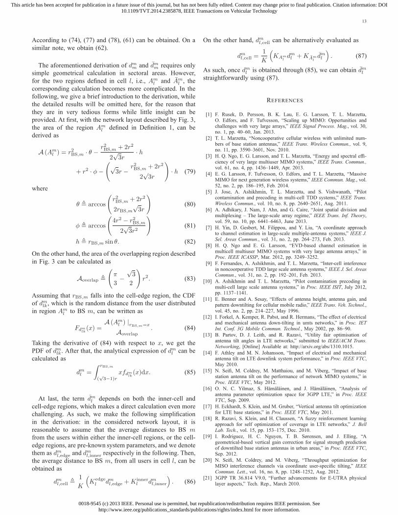
The aforementioned derivation of dmm and dmm requires only

simple geometrical calculation in sectoral areas. However,

for the two regions defined in cell l, i.e., Aml and Am

l , the

corresponding calculation becomes more complicated. In the

following, we give a brief introduction to the derivation, while

the detailed results will be omitted here, for the reason that

they are in very tedious forms while little insight can be

provided. At first, with the network layout described by Fig. 3,

the area of the region Aml defined in Definition 1, can be

derived as

A (Aml ) = r2BS,m · θ −

r2BS,m + 2r2

2√3r

· h

+ r2 · φ−(

√3r −

r2BS,m + 2r2

2√3r

)

· h (79)

where

θ , arccos

(

r2BS,m + 2r2

2rBS,m

√3r

)

(80)

φ , arccos

(

4r2 − r2BS,m

2√3r2

)

(81)

h , rBS,m sin θ. (82)

On the other hand, the area of the overlapping region described

in Fig. 3 can be calculated as

Aoverlap ,

(

π

3−√3

2

)

r2. (83)

Assuming that rBS,m falls into the cell-edge region, the CDF

of dmlk , which is the random distance from the user distributed

in region Aml to BS m, can be written as

Fdmlk(x) =

A (Aml ) |rBS,m=x

Aoverlap. (84)

Taking the derivative of (84) with respect to x, we get the

PDF of dmlk . After that, the analytical expression of dml can be

calculated as

dml =

∫ rBS,m

(√3−1)r

xfdmlk(x)dx. (85)

At last, the term dml depends on both the inner-cell and

cell-edge regions, which makes a direct calculation even more

challenging. As such, we make the following simplification

in the derivation: in the considered network layout, it is

reasonable to assume that the average distances to BS m

from the users within either the inner-cell regions, or the cell-

edge regions, are pre-known system parameters, and we denote

them as dml,edge and dml,inner respectively in the following. Then,

the average distance to BS m, from all users in cell l, can be

obtained as

dml,cell ,1

K

(

Kedgel dml,edge +K inner

l dml,inner

)

. (86)

On the other hand, dml,cell can be alternatively evaluated as

dml,cell =1

K

(

KAmldml +KAm

ldml

)

. (87)

As such, once dml is obtained through (85), we can obtain dmlstraightforwardly using (87).

REFERENCES

[1] F. Rusek, D. Persson, B. K. Lau, E. G. Larsson, T. L. Marzetta,O. Edfors, and F. Tufvesson, “Scaling up MIMO: Oppertunities andchallenges with very large arrays,” IEEE Signal Process. Mag., vol. 30,no. 1, pp. 40–60, Jan. 2013.

[2] T. L. Marzetta, “Noncooperative cellular wireless with unlimited num-bers of base station antennas,” IEEE Trans. Wireless Commun., vol. 9,no. 11, pp. 3590–3601, Nov. 2010.

[3] H. Q. Ngo, E. G. Larsson, and T. L. Marzetta, “Energy and spectral effi-ciency of very large multiuser MIMO systems,” IEEE Trans. Commun.,vol. 61, no. 4, pp. 1436–1449, Apr. 2013.

[4] E. G. Larsson, F. Tufvesson, O. Edfors, and T. L. Marzetta, “MassiveMIMO for next generation wireless systems,” IEEE Commun. Mag., vol.52, no. 2, pp. 186–195, Feb. 2014.

[5] J. Jose, A. Ashikhmin, T. L. Marzetta, and S. Vishwanath, “Pilotcontamination and precoding in multi-cell TDD systems,” IEEE Trans.Wireless Commun., vol. 10, no. 8, pp. 2640–2651, Aug. 2011.

[6] A. Adhikary, J. Nam, J. Ahn, and G. Caire, “Joint spatial division andmultiplexing – The large-scale array regime,” IEEE Trans. Inf. Theory,vol. 59, no. 10, pp. 6441–6463, June 2013.

[7] H. Yin, D. Gesbert, M. Filippou, and Y. Liu, “A coordinate approachto channel estimation in large-scale multiple-antenna systems,” IEEE J.Sel. Areas Commun., vol. 31, no. 2, pp. 264–273, Feb. 2013.

[8] H. Q. Ngo and E. G. Larsson, “EVD-based channel estimation inmulticell multiuser MIMO systems with very large antenna arrays,” inProc. IEEE ICASSP, Mar. 2012, pp. 3249–3252.

[9] F. Fernandes, A. Ashikhmin, and T. L. Marzetta, “Inter-cell inteferencein noncoorperative TDD large scale antenna systems,” IEEE J. Sel. AreasCommun., vol. 31, no. 2, pp. 192–201, Feb. 2013.

[10] A. Ashikhmin and T. L. Marzetta, “Pilot contamination precoding inmulti-cell large scale antenna systems,” in Proc. IEEE ISIT, July 2012,pp. 1137–1141.

[11] E. Benner and A. Sesay, “Effects of antenna height, antenna gain, andpattern downtilting for cellular mobile radio,” IEEE Trans. Veh. Technol.,vol. 45, no. 2, pp. 214–227, May 1996.

[12] I. Forkel, A. Kemper, R. Pabst, and R. Hermans, “The effect of electricaland mechanical antenna down-tilting in umts networks,” in Proc. IETInt. Conf. 3G Mobile Commun. Technol., May 2002, pp. 86–90.

[13] B. Partov, D. J. Leith, and R. Razavi, “Utility fair optimisation ofantenna tilt angles in LTE networks,” submitted to IEEE/ACM Trans.Networking, [Online] Available at: http://arxiv.org/abs/1310.1015.

[14] F. Athley and M. N. Johansson, “Impact of electrical and mechanicalantenna tilt on LTE downlink system performance,” in Proc. IEEE VTC,May 2010.

[15] N. Seifi, M. Coldrey, M. Matthaiou, and M. Viberg, “Impact of basestation antenna tilt on the performance of network MIMO systems,” inProc. IEEE VTC, May 2012.

[16] O. N. C. Yilmaz, S. Hamalainen, and J. Hamalainen, “Analysis ofantenna parameter optimization space for 3GPP LTE,” in Proc. IEEEVTC, Sep. 2009.

[17] H. Eckhardt, S. Klein, and M. Gruber, “Vertical antenna tilt optimizationfor LTE base stations,” in Proc. IEEE VTC, May 2011.

[18] R. Razavi, S. Klein, and H. Claussen, “A fuzzy reinforcement learningapproach for self optimization of coverage in LTE networks,” J. BellLab. Tech., vol. 15, pp. 153–175, Dec. 2010.

[19] I. Rodriguez, H. C. Nguyen, T. B. Sørensen, and J. Elling, “Ageometrical-based vertical gain correction for signal strength predictionof downtilted base station antennas in urban areas,” in Proc. IEEE VTC,Sep. 2012.

[20] N. Seifi, M. Coldrey, and M. Viberg, “Throughput optimization forMISO interference channels via coordinate user-specific tilting,” IEEECommun. Lett., vol. 16, no. 8, pp. 1248–1252, Aug. 2012.

[21] 3GPP TR 36.814 V9.0, “Further advancements for E-UTRA physicallayer aspects,” Tech. Rep., March 2010.



14

[22] Y.-H. Nam, B. L. Ng, K. Sayana, Y. Li, J. Zhang, Y. Kim and J.Lee, “Full dimension MIMO (FD-MIMO) for next generation cellulartechnology,” IEEE Commun. Mag., vol. 51, no. 6, pp. 172–179, June2013.

[23] T. Q. S. Quek, G. de la Roche, I. Guvenc, and M. Kountouris, “Smallcell networks: Deployment, PHY techniques, and resource allocation,”Cambridge University Press, 2013.

[24] R. Pabst et. al., “Relay-based deployment concepts for wireless andmobile broadband radio,” IEEE Commun. Mag., vol. 42, no. 9, pp. 80–89, Sep. 2004.

[25] Y. Zhuang, Y. Luo, L. Cai, and J. Pan, “A geometric probability modelfor capacity analysis and interference estimation in wireless mobilecellular systems,” in Proc. IEEE GLOBECOM, Dec. 2011.

[26] A. Goldsmith, Wireless Communications, Cambridge University Press,New York, 2005.

[27] A. Lozano, R. W. Heath Jr., and J. G. Andrews, “Fundamental limits ofcooperation,” IEEE Trans. Inf. Theory, vol. 59, no. 9, pp. 5213–5226,Sep. 2013.

Shi Jin (S’06-M’07) received the B.S. degree incommunications engineering from Guilin Universityof Electronic Technology, Guilin, China, in 1996, theM.S. degree from Nanjing University of Posts andTelecommunications, Nanjing, China, in 2003, andthe Ph.D. degree in communications and informationsystems from the Southeast University, Nanjing, in2007. From June 2007 to October 2009, he was aResearch Fellow with the Adastral Park ResearchCampus, University College London, London, U.K.He is currently with the faculty of the National Mo-

bile Communications Research Laboratory, Southeast University. His researchinterests include space time wireless communications, random matrix theory,and information theory. He serves as an Associate Editor for the IEEETRANSACTIONS ON WIRELESS COMMUNICATIONS, IEEE COMMUNICA-TIONS LETTERS, and IET COMMUNICATIONS. Dr. Jin and his co-authorshave been awarded the 2011 IEEE Communications Society Stephen O. RicePrize Paper Award in the field of communication theory and a 2010 YoungAuthor Best Paper Award by the IEEE Signal Processing Society.

Jue Wang (S’10 - M’14) received the B.S. degree incommunications engineering from Nanjing Univer-sity, Nanjing, China, in 2006, the M.S. degree andPh. D. degree from the National CommunicationsResearch Laboratory, Southeast University, Nanjing,China, respectively in 2009 and 2014.In 2014, he joined the School of Electronic

and Information Engineering, Nantong University.Meanwhile, he is with Singapore University of Tech-nology and Design (SUTD) as a post-doctoral re-search fellow. His research interests include MIMO

wireless communications, multiuser transmission, MIMO channel modeling,massive MIMO systems and physical layer security.

Qiang Sun (S’10) received the Ph.D. degreein Communication and Information System fromSoutheast University, Nanjing, China, in 2014. Hejoined the School of Electronic and InformationEngineering, Nantong University, Nantong, China,in April 2006. Now he is a lecturer of informationsystems and communications. His current researchinterests include massive MIMO and small cell net-works.

Michail Matthaiou (S’05–M’08–SM’13) was bornin Thessaloniki, Greece in 1981. He obtained theDiploma degree (5 years) in Electrical and Com-puter Engineering from the Aristotle University ofThessaloniki, Greece in 2004. He then received theM.Sc. (with distinction) in Communication Systemsand Signal Processing from the University of Bristol,U.K. and Ph.D. degrees from the University ofEdinburgh, U.K. in 2005 and 2008, respectively.From September 2008 through May 2010, he waswith the Institute for Circuit Theory and Signal

Processing, Munich University of Technology (TUM), Germany working as aPostdoctoral Research Associate. He is currently a Senior Lecturer at Queen’sUniversity Belfast, U.K. and also holds an adjunct Assistant Professor positionat Chalmers University of Technology, Sweden. His research interests spansignal processing for wireless communications, massive MIMO, hardware-constrained communications, and performance analysis of fading channels.Dr. Matthaiou is the recipient of the 2011 IEEE ComSoc Best Young

Researcher Award for the Europe, Middle East and Africa Region and aco-recipient of the 2006 IEEE Communications Chapter Project Prize forthe best M.Sc. dissertation in the area of communications. He was co-recipient of the Best Paper Award at the 2014 IEEE International Con-ference on Communications (ICC) and was an Exemplary Reviewer forIEEE COMMUNICATIONS LETTERS for 2010. He has been a member ofTechnical Program Committees for several IEEE conferences such as ICC,GLOBECOM, VTC etc. He currently serves as an Associate Editor for theIEEE TRANSACTIONS ON COMMUNICATIONS, IEEE COMMUNICATIONS

LETTERS and was the Lead Guest Editor of the special issue on “Large-scalemultiple antenna wireless systems” of the IEEE JOURNAL ON SELECTEDAREAS IN COMMUNICATIONS. He is an associate member of the IEEE SignalProcessing Society SPCOM and SAM technical committees.

Xiqi Gao (SM’07–F’14) received the Ph.D. degreein electrical engineering from Southeast University,Nanjing, China, in 1997. He joined the Departmentof Radio Engineering, Southeast University, in April1992. Since May 2001, he has been a professorof information systems and communications. FromSeptember 1999 to August 2000, he was a visitingscholar at Massachusetts Institute of Technology,Cambridge, and Boston University, Boston, MA.From August 2007 to July 2008, he visited theDarmstadt University of Technology, Darmstadt,

Germany, as a Humboldt scholar. His current research interests includebroadband multicarrier communications, MIMO wireless communications,channel estimation and turbo equalization, and multirate signal processingfor wireless communications. He serves as an Associate Editor for the IEEETRANSACTIONS ON SIGNAL PROCESSING and the IEEE TRANSACTIONSON WIRELESS COMMUNICATIONS. Dr. Gao received the Science and Tech-nology Awards of the State Education Ministry of China in 1998, 2006 and2009, the National Technological Invention Award of China in 2011, and the2011 IEEE Communications Society Stephen O. Rice Prize Paper Award inthe field of communications theory.

Documents

Cell Coverage Optimization for the Multicell Massive MIMO ... · Index Terms —Cellcoverage,massiveMIMO,pilotcontamina-tion,uplink. I. INTRODUCTION Massive multiple-input multiple-output