Embed Size (px)
Citation preview
Portland State University Portland State University
PDXScholar PDXScholar
Civil and Environmental Engineering Faculty Publications and Presentations Civil and Environmental Engineering
7-2000
CE-QUAL-W2, Version 3 CE-QUAL-W2, Version 3
Scott A. Wells Portland State University
Thomas M. Cole U.S. Army Engineer Research and Development Center
Follow this and additional works at: https://pdxscholar.library.pdx.edu/cengin_fac
Part of the Hydrology Commons, and the Water Resource Management Commons
Let us know how access to this document benefits you.
Citation Details Citation Details Wells, S. A., and Cole, T. M. (2000). “CE-QUAL-W2, Version 3,” Water Quality Technical Notes Collection (ERDC WQTN-AM-09), U.S. Army Engineer Research and Development Center, Vicksburg, MS. www.wes.army.mil/el/elpubs/wqtncont.html
This Technical Report is brought to you for free and open access. It has been accepted for inclusion in Civil and Environmental Engineering Faculty Publications and Presentations by an authorized administrator of PDXScholar. Please contact us if we can make this document more accessible: [email protected].
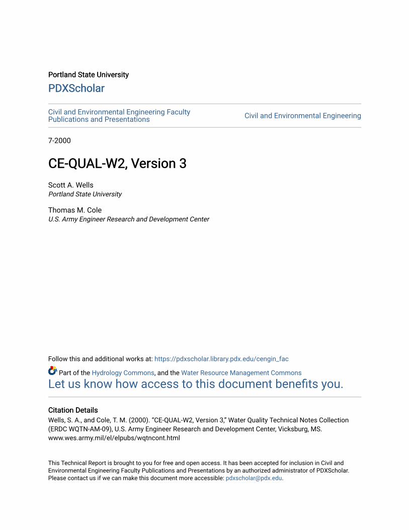
INTRODUCTION: CE-QUAL-W2 is a two-dimensional water quality and hydrodynamic codesupported by the U.S. Army Enginer Research and Development Center (Cole and Buchak 1995).The model has been widelyapplied to stratified surfacewater systems such as lakes,reservoirs, and estuaries andcomputes water levels, hori-zontal and vertical velocities,temperature, and 21 otherwater quality parameters(such as dissolved oxygen,nutrients, organic matter, al-gae, pH, the carbonate cycle,bacteria, and dissolved andsuspended solids). A typicalmodel grid is shown in Fig-ure 1 where the vertical axisis aligned with gravity.
This technical note documents the development of CE-QUAL-W2, Version 3, which incorporatessloping riverine sections. Version 3 has the capability of modeling entire river basins with riversand interconnected lakes, reservoirs, and/or estuaries. Four example applications illustrate the useof Version 3.
DEVELOPMENT RATIONALE: CE-QUAL-W2 has been in use for the last two decades as atool for water quality managers to assess the impacts of management strategies on reservoir, lake,and estuarine systems. A predominant feature of the model is its ability to compute the two-dimensional velocity field for narrow systems that stratify. In contrast with many reservoir modelsthat are zero-dimensional with regards to hydrodynamics, the ability to accurately simulate transportcan be as important as the water column kinetics in accurately simulating water quality.
A limitation of Version 2 is its inability to model sloping riverine waterbodies. Models such asWQRSS (Smith 1978), HEC-5Q, and HSPF (Donigian et al. [1984), have been developed for riverbasin modeling but have serious limitations. One issue is that the HEC-5Q (similar to WQRSS)and HSPF models incorporate a one-dimensional (1-D), longitudinal river model with a 1-D, verticalreservoir model (1-D for temperature and water quality and zero-dimensional for hydrodynamics).The modeler must choose the location of the transition from 1-D longitudinal to 1-D vertical. Besidesthe limitation of not solving for the velocity field in the stratified reservoir system, any point sourceinputs to the reservoir section are spread over the entire longitudinal distribution of the reservoirlayer.
ERDC WQTN-AM-09July 2000
CE-QUAL-W2, Version 3
by Scott A. Wells and Thomas M. Cole
Figure 1. Typical CE-QUAL-W2, Version 2 model grid
1
Other hydraulic and water quality models commonly used for unsteady flow include the 1-Ddynamic EPA model DYNHYD (Ambrose et al. 1988), used with the multidimensional waterquality model WASP. WASP relies on DYNHYD for 1-D hydrodynamic predictions. If WASP isused in a multidimensional schematization, the modeler must specify dispersion coefficients toallow transport in the vertical and/or lateral directions or use another hydrodynamic model thatexplicitly includes these effects. In addition, the Corps model CE-QUAL-RIV1 (EnvironmentalLaboratory 1995), is a 1-D dynamic flow and water quality model used for 1-D river or streamsections. None of these models have the ability to characterize adequately the hydraulics or waterquality of deeper reservoir systems or deep river pools that stratify.
In the original development of CE-QUAL-W2, vertical accelerations were considered negligiblecompared to gravity forces. This assumption led to the hydrostatic pressure approximation for thez-momentum equation. In sloping channels, this assumption is not always valid because verticalaccelerations cannot be neglected if the z-axis is aligned with gravity. In addition, the currentVersion 2 algorithm does not allow the upstream bed elevation to be above the downstream watersurface elevation. Because watershed and river basin modeling are becoming more important forwater quality managers, providing the capability for CE-QUAL-W2 to be used as a complete toolfor river basin modeling is an essential step in improving the current state of the art.
DEVELOPMENT APPROACH: There were many approaches that could have been imple-mented to incorporate riverine branches within CE-QUAL-W2. By choosing a theoretical basis forthe riverine branches that uses the existing CE-QUAL-W2 two-dimnesional (2-D) computationalscheme for hydraulics and water quality, the following benefits accrued:
• Code updates in the computational scheme affected the entire model rather than just one ofthe computational schemes for either the riverine or the reservoir sections, leading to eas-ier code maintenance.
• No changes were made to the temperature or water quality solution algorithms.• By using the two-dimensional framework, the riverine branches had the ability to predict
the velocity and water quality field in two dimensions - this has advantages in modelingthe following processes: sediment deposition and scour, particulate (algae, detritus, sus-pended solids) sedimentation, and sediment flux processes as well as making Manning’sfriction factor stage invariant (see Wells (1999)).
• Since the entire watershed model had the same theoretical basis, setting up branches andinterfacing branches involved the same process whether for reservoir or riverine sections,thus making code maintenance and model setup easier.
The theoretical approach was to re-derive the governing equations assuming that the 2-D grid isadjusted by the channel slope (Figure 2).
ERDC WQTN-AM-09July 2000
2

THEORETICAL BASIS: Details of deriving the governing equations for CE-QUAL-W2,Version 3 for the river basin model are given in Wells (1997). Table 1 shows the governingequations after lateral averaging for a channel slope of zero (original model formulation) and foran arbitrary channel slope.
Figure 2. Conceptual schematic of river-reservoir connection
Table 1Comparison of Governing Equations for CE-QUAL-W2 with and withoutChannel Slope
Note: U,W: horizontal and vertical velocity, B: channel width, P: pressure, g: acceleration due togravity, τ x,τ z: lateral average shear stress in x and z, ρ : density, η : water surface, α : channel angle,Ux: x-component of velocity from side branch, q: lateral inflow per unit length
ERDC WQTN-AM-09July 2000
3
Numerous algorithmic changes were made in the CE-QUAL-W2 model. In addition to the generalchannel sloping feature, these changes include:
a. Ability to choose the following:
• Turbulence closure models for each waterbody using eddy-viscosity mixing lengthmodels.
• Varying vertical grids between waterbodies.• Chezy or Manning’s friction factor.• Reaeration formulae based on the riverine or reservoir/lake or estuary character of the
waterbody or user-defined formulations.• Evaporation models based on theory or user-defined formulations
b. Ability to linearly link one branch with another or specify an internal dam or internalhydraulic structure(s) (spillways, gates, weirs, and pipes) within or between water bodies(the pipes algorithm is an unsteady 1-D hydrodynamic sub-model to the core W2 codefrom Berger and Wells (1999).
c. Effect of hydraulic structures on gas transfer and total dissolved gas transport.
d. Conservation of longitudinal momentum at intersections between main branches and sidebranches.
e. Effect of lateral inflows from tributaries or the lateral component of inflows from branchintersections on the vertical eddy viscosity.
f. QUICKEST/ULTIMATE numerical transport scheme.
g. Implicit eddy viscosity formulation that removes its timestep requirement.
h. Multiple user-defined algal groups.
i. Multiple user-defined organic matter groups.
j. Sediment diagenesis model.
TEST APPLICATIONS
Richard B. Russell (RBR)/J. Strom Thurmond (JST). RBR and JST (previously known asClarks Hill Lake as shown in Figure 3) are Corps reservoirs located on the Savannah River betweenGeorgia and South Carolina. JST is located immediately below RBR. The study involved investi-gating the effects of proposed pump-storage operations on temperature and water quality for thetwo reservoirs. This required a rewrite of the code in order to dynamically link the two systems.The linkage algorithm was sufficiently generalized to allow dynamic linkage to any number of“waterbodies.” During algorithm development, it was recognized that a natural extension wouldbe to allow modeling of the river reaches between reservoirs, thus providing a state-of-the-art
ERDC WQTN-AM-09July 2000
4
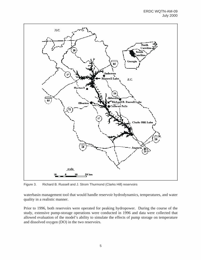
waterbasin management tool that would handle reservoir hydrodynamics, temperatures, and waterquality in a realistic manner.
Prior to 1996, both reservoirs were operated for peaking hydropower. During the course of thestudy, extensive pump-storage operations were conducted in 1996 and data were collected thatallowed evaluation of the model’s ability to simulate the effects of pump storage on temperatureand dissolved oxygen (DO) in the two reservoirs.
Figure 3. Richard B. Russell and J. Strom Thurmond (Clarks Hill) reservoirs
ERDC WQTN-AM-09July 2000
5
All hydrodynamic/temperature calibration parameters, including longitudinal eddy viscosity/diffusivity, bottom friction, sediment heat exchange, and short wave solar radiation absorption/extinction, were set to their default values with the exception of the wind-sheltering coefficient,which was set to 0.9 for RBR and 1.0 for JST. The wind-sheltering coefficient is used to multiplyobserved winds in order to decrease the effective wind reaching the reservoir surface.
Temperature simulations. The model was calibrated to data collected during 1988, 1994, and 1996.The year 1988 represents a low-flow year, 1994 represents a high-flow year, and 1996 representsan average flow year with extensive pump-storage operations.
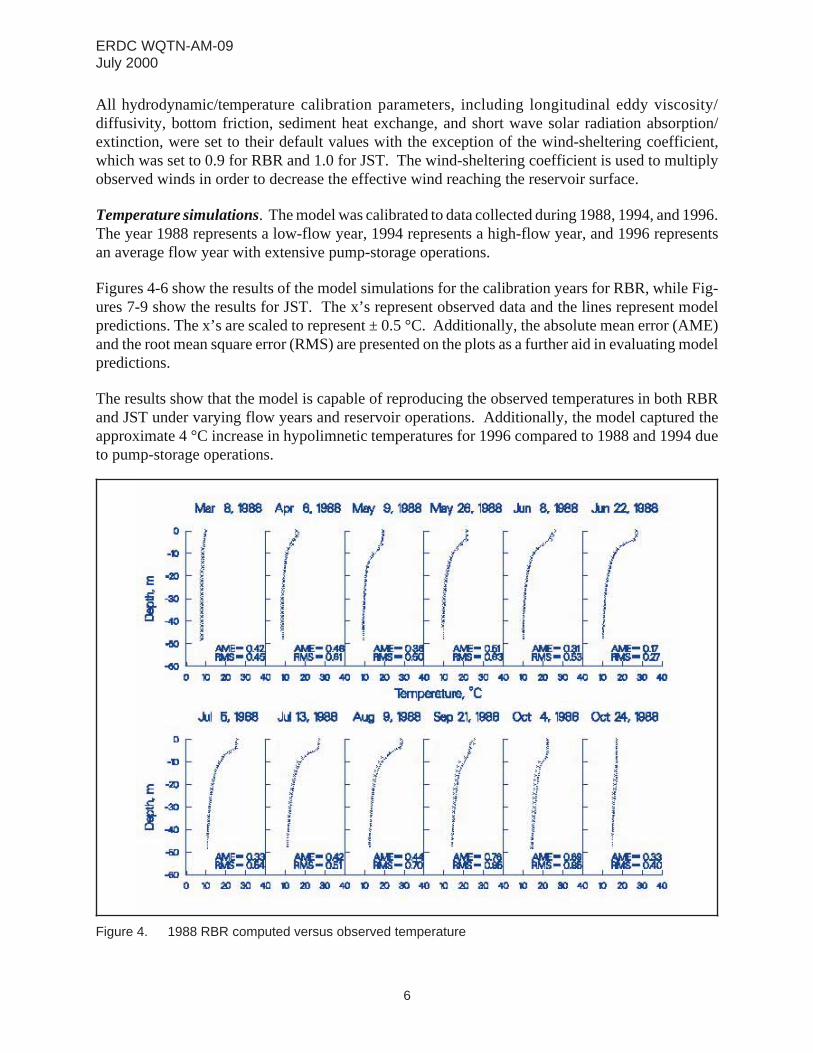
Figures 4-6 show the results of the model simulations for the calibration years for RBR, while Fig-ures 7-9 show the results for JST. The x’s represent observed data and the lines represent modelpredictions. The x’s are scaled to represent ± 0.5 °C. Additionally, the absolute mean error (AME)and the root mean square error (RMS) are presented on the plots as a further aid in evaluating modelpredictions.
The results show that the model is capable of reproducing the observed temperatures in both RBRand JST under varying flow years and reservoir operations. Additionally, the model captured theapproximate 4 °C increase in hypolimnetic temperatures for 1996 compared to 1988 and 1994 dueto pump-storage operations.
Figure 4. 1988 RBR computed versus observed temperature
ERDC WQTN-AM-09July 2000
6
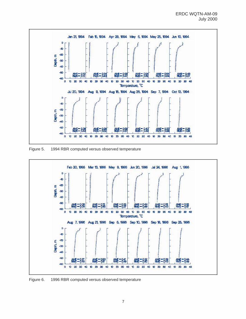
Figure 5. 1994 RBR computed versus observed temperature
Figure 6. 1996 RBR computed versus observed temperature
ERDC WQTN-AM-09July 2000
7
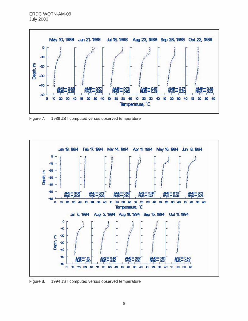
Figure 7. 1988 JST computed versus observed temperature
Figure 8. 1994 JST computed versus observed temperature
ERDC WQTN-AM-09July 2000
8
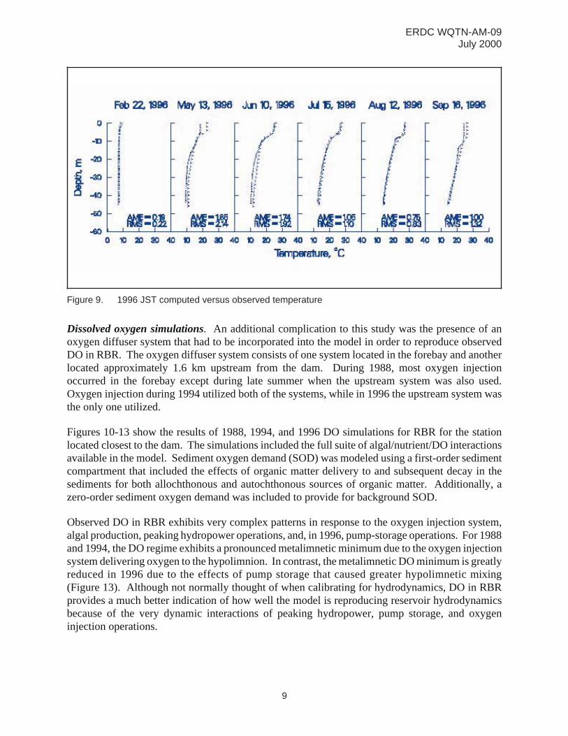
Dissolved oxygen simulations. An additional complication to this study was the presence of anoxygen diffuser system that had to be incorporated into the model in order to reproduce observedDO in RBR. The oxygen diffuser system consists of one system located in the forebay and anotherlocated approximately 1.6 km upstream from the dam. During 1988, most oxygen injectionoccurred in the forebay except during late summer when the upstream system was also used.Oxygen injection during 1994 utilized both of the systems, while in 1996 the upstream system wasthe only one utilized.
Figures 10-13 show the results of 1988, 1994, and 1996 DO simulations for RBR for the stationlocated closest to the dam. The simulations included the full suite of algal/nutrient/DO interactionsavailable in the model. Sediment oxygen demand (SOD) was modeled using a first-order sedimentcompartment that included the effects of organic matter delivery to and subsequent decay in thesediments for both allochthonous and autochthonous sources of organic matter. Additionally, azero-order sediment oxygen demand was included to provide for background SOD.
Observed DO in RBR exhibits very complex patterns in response to the oxygen injection system,algal production, peaking hydropower operations, and, in 1996, pump-storage operations. For 1988and 1994, the DO regime exhibits a pronounced metalimnetic minimum due to the oxygen injectionsystem delivering oxygen to the hypolimnion. In contrast, the metalimnetic DO minimum is greatlyreduced in 1996 due to the effects of pump storage that caused greater hypolimnetic mixing(Figure 13). Although not normally thought of when calibrating for hydrodynamics, DO in RBRprovides a much better indication of how well the model is reproducing reservoir hydrodynamicsbecause of the very dynamic interactions of peaking hydropower, pump storage, and oxygeninjection operations.
Figure 9. 1996 JST computed versus observed temperature
ERDC WQTN-AM-09July 2000
9

Figure 10. 1988 RBR computed versus observed DO, March-June
Figure 11. 1988 RBR computed versus observed DO, June-October
ERDC WQTN-AM-09July 2000
10
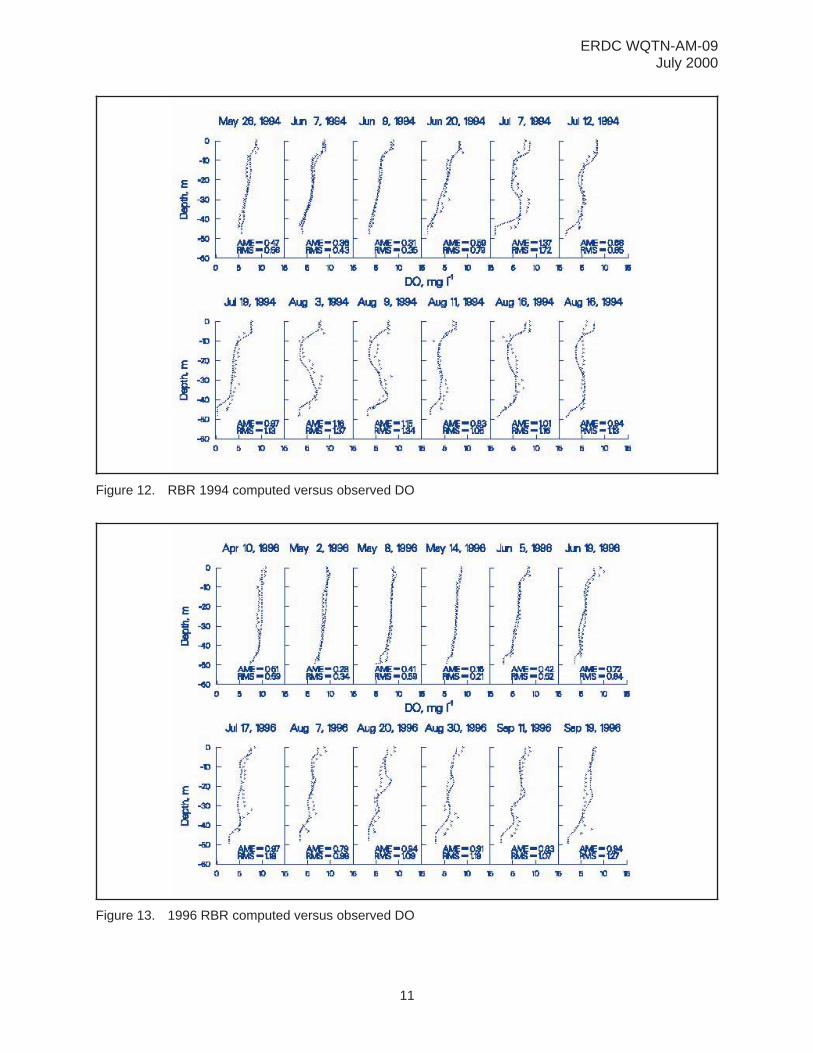
Figure 12. RBR 1994 computed versus observed DO
Figure 13. 1996 RBR computed versus observed DO
ERDC WQTN-AM-09July 2000
11
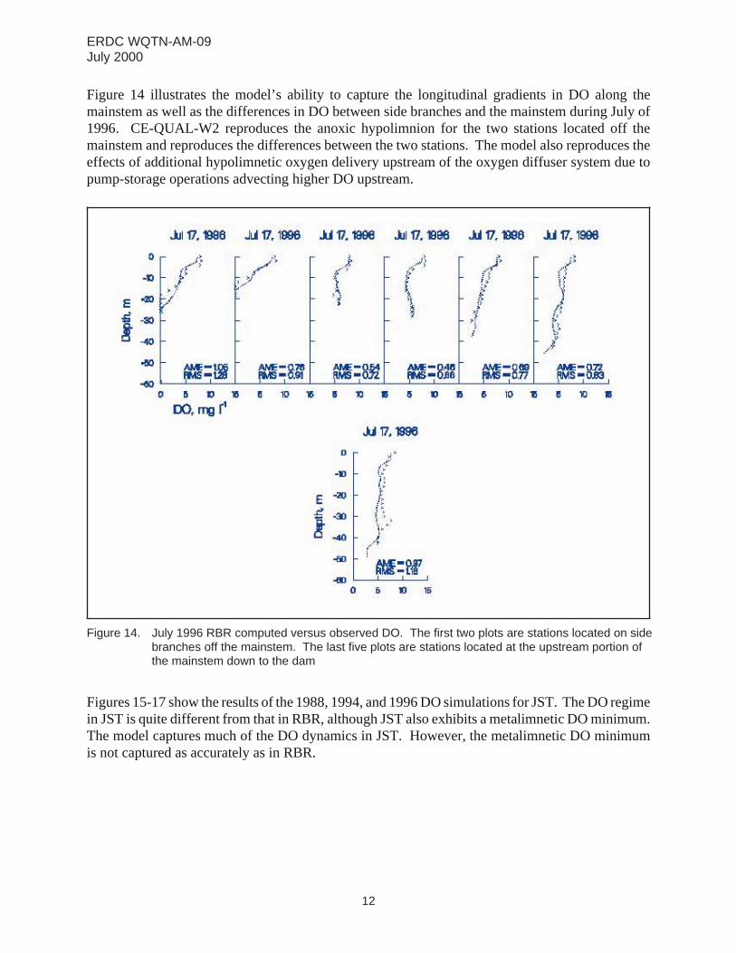
Figure 14 illustrates the model’s ability to capture the longitudinal gradients in DO along themainstem as well as the differences in DO between side branches and the mainstem during July of1996. CE-QUAL-W2 reproduces the anoxic hypolimnion for the two stations located off themainstem and reproduces the differences between the two stations. The model also reproduces theeffects of additional hypolimnetic oxygen delivery upstream of the oxygen diffuser system due topump-storage operations advecting higher DO upstream.
Figures 15-17 show the results of the 1988, 1994, and 1996 DO simulations for JST. The DO regimein JST is quite different from that in RBR, although JST also exhibits a metalimnetic DO minimum.The model captures much of the DO dynamics in JST. However, the metalimnetic DO minimumis not captured as accurately as in RBR.
Figure 14. July 1996 RBR computed versus observed DO. The first two plots are stations located on sidebranches off the mainstem. The last five plots are stations located at the upstream portion ofthe mainstem down to the dam
ERDC WQTN-AM-09July 2000
12

Figure 15. 1988 JST computed versus observed DO
Figure 16. 1994 JST computed versus observed DO
ERDC WQTN-AM-09July 2000
13

Lower Snake River. The domain of the Lower Snake River from C. J. Strike Reservoir (RM487) to the headwaters of Brownlee Reservoir (RM 335) is 244 km (152 miles) in length. The riverwas broken into five branches of varying slope from 0.001 to 0.0008 (Figure 18). The modelconsisted of 312 longitudinal segments between 805 and 835 m in length, 13 tributary and pointsources, 1 distributed load, and 90 agricultural return flows.
Hydraulics were calibrated using water surface elevation data at specific flow rates. Gauging stationdata were available at several locations throughout the domain. Figure 19 shows the water levelcalibration for a flow of 5,600 cfs. Mean water level error and root mean square water level errorfor flow rates between 5,600 cfs and 13,000 cfs were well below 0.5 ft for a river that experiencesa 300-ft drop over its length. The calibrated Chezy values varied from segment to segment between20 and 80 and were flow and stage invariant.
The primary goal of this modeling study was to determine the loading of organic matter and nutrientsto Brownlee Reservoir. Model predictions of temperature, algae, nutrients, and organic mattercompared well with field data at six locations along the river. Results from the Porter’s Island stationare given in Figures 20-23.
Bull Run River System. The Bull Run watershed has been the primary drinking water supplysince 1895 for the metropolitanarea of Portland, OR, USA. The watershed is composed of two
Figure 17. 1996 JST computed versus observed DO
ERDC WQTN-AM-09July 2000
14
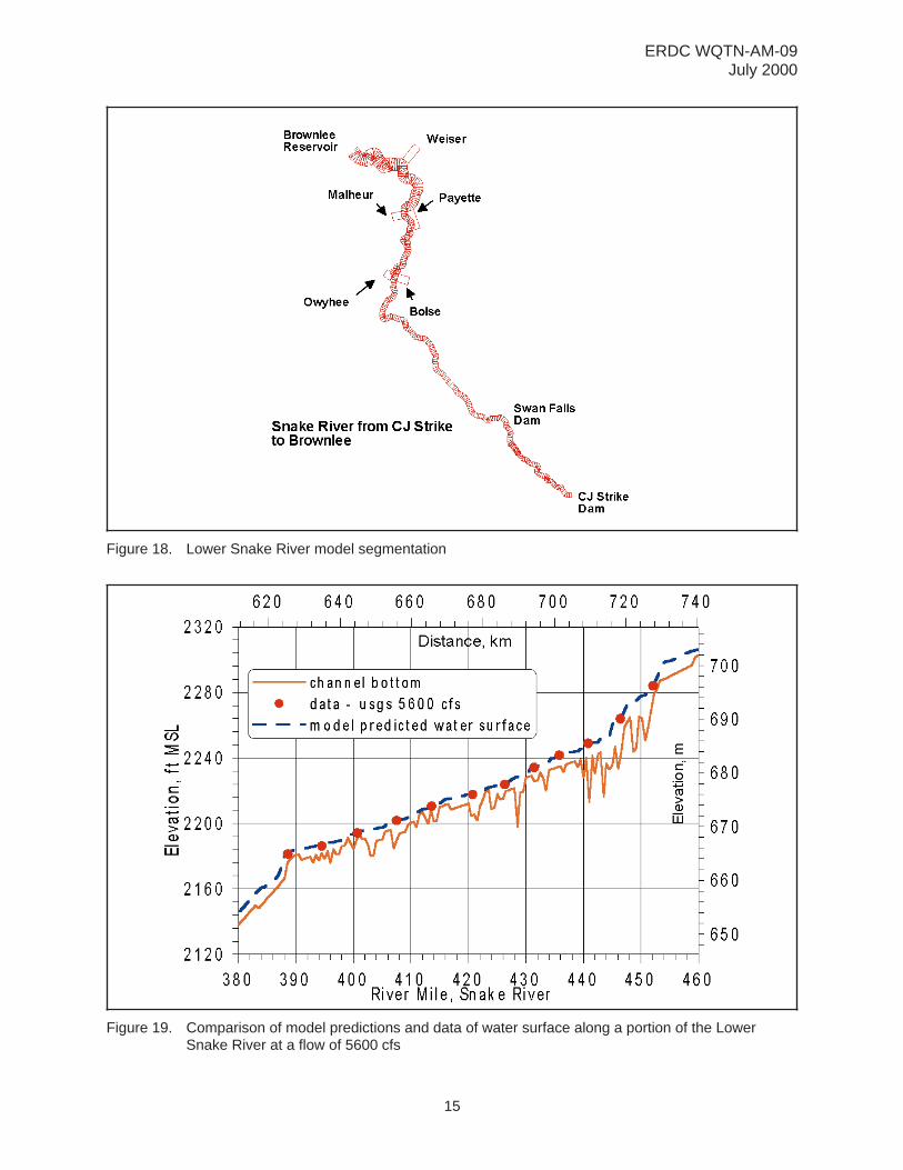
Figure 18. Lower Snake River model segmentation
Figure 19. Comparison of model predictions and data of water surface along a portion of the LowerSnake River at a flow of 5600 cfs
ERDC WQTN-AM-09July 2000
15

Figure 20. Computed versus observed temperatures
Figure 21. Computed versus observed chlorophyll a
ERDC WQTN-AM-09July 2000
16
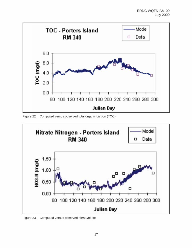
Figure 22. Computed versus observed total organic carbon (TOC)
Figure 23. Computed versus observed nitrate/nitrite
ERDC WQTN-AM-09July 2000
17
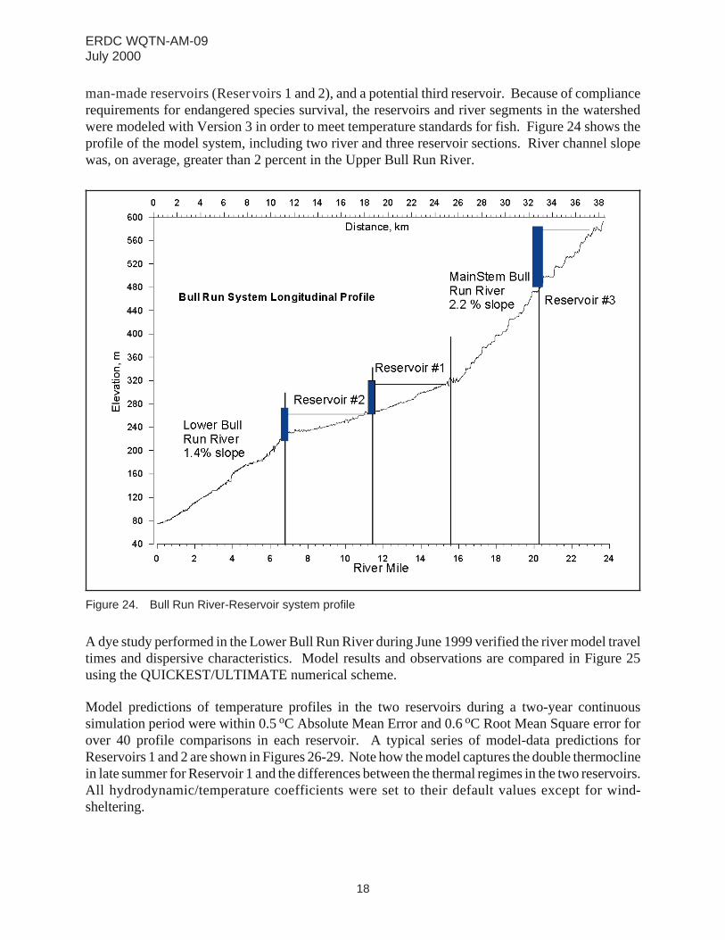
man-made reservoirs (Reservoirs1 and 2), and a potential third reservoir. Because of compliancerequirements for endangered species survival, the reservoirs and river segments in the watershedwere modeled with Version 3 in order to meet temperature standards for fish. Figure 24 shows theprofile of the model system, including two river and three reservoir sections. River channel slopewas, on average, greater than 2 percent in the Upper Bull Run River.
A dye study performed in the Lower Bull Run River during June 1999 verified the river model traveltimes and dispersive characteristics. Model results and observations are compared in Figure 25using the QUICKEST/ULTIMATE numerical scheme.
Model predictions of temperature profiles in the two reservoirs during a two-year continuoussimulation period were within 0.5oC Absolute Mean Error and 0.6oC Root Mean Square error forover 40 profile comparisons in each reservoir. A typical series of model-data predictions forReservoirs 1 and 2 are shown in Figures 26-29. Note how the model captures the double thermoclinein late summer for Reservoir 1 and the differences between the thermal regimes in the two reservoirs.All hydrodynamic/temperature coefficients were set to their default values except for wind-sheltering.
Figure 24. Bull Run River-Reservoir system profile
ERDC WQTN-AM-09July 2000
18
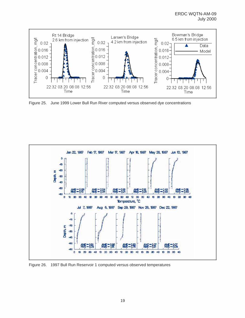
Figure 25. June 1999 Lower Bull Run River computed versus observed dye concentrations
Figure 26. 1997 Bull Run Reservoir 1 computed versus observed temperatures
ERDC WQTN-AM-09July 2000
19
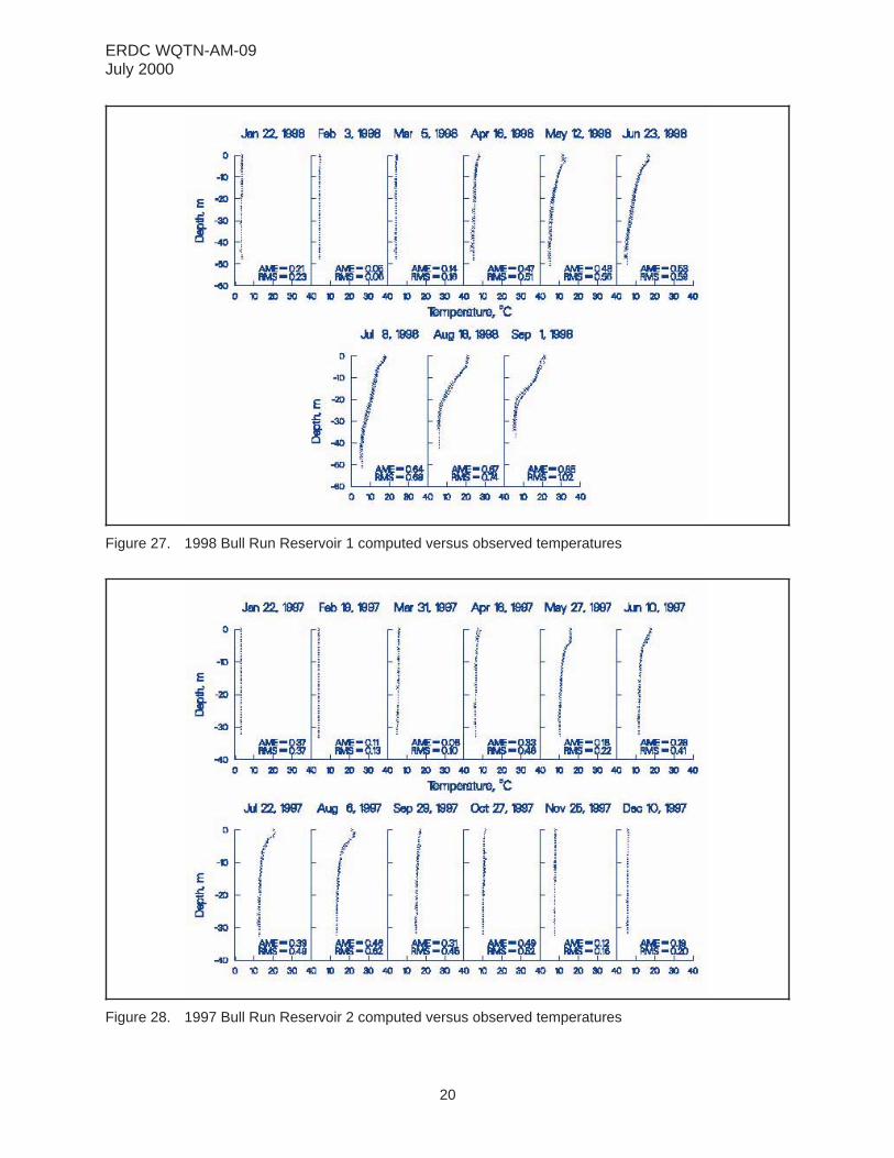
Figure 27. 1998 Bull Run Reservoir 1 computed versus observed temperatures
Figure 28. 1997 Bull Run Reservoir 2 computed versus observed temperatures
ERDC WQTN-AM-09July 2000
20

Columbia Slough System. The Columbia Slough (Figure 30) is an extensive system ofinterconnected wetlands, channels, and lakes located in the Portland, Oregon, USA metropolitanarea and lying in the floodplain of the Columbia River. It is approximately 30 km in length andincludes a freshwater estuary portion and a series of isolated lakes and channels that receivestormwater and groundwater inflows. The model was developed to evaluate the effect of combinedsewer overflows, stormwater, and groundwater inflows on water quality in the Columbia Sloughsystem. Model development is summarized in Berger and Wells (1999).
The Lower Columbia Slough (Figure 31) is connected to the Willamette River, where it experiencesa water surface fluctuation between 1 and 3 ft. Inflows to the Lower Columbia Slough includecombined-sewer-overflows (CSOs), storm water, water from Smith and Bybee Lakes, leachate fromthe St. John’s Landfill, and inflows (both pumped and gravity inflows) from the Upper ColumbiaSlough at MCDD1.
The Upper Columbia Slough, shown in Figure 32, was historically maintained to provide irrigationwater to agricultural and commercial users in the summer months. The Upper Slough is connectedby pipes and an overflow weir during the fall, winter, and spring to Fairview Lake. During thesummer, Fairview Lake is connected to the Upper Slough only by flow over and leakage throughthe weir. Water is also pumped from the Upper Slough to the Lower Columbia Slough at a pumpstation at MCDD1(MultnomahCountyDrainageDistrict No. 1) and from the Upper Slough to theColumbia River at MCDD4(MultnomahCountyDrainageDistrict No. 4). At MCDD1, pipes alsoallow gravity flow from the Upper Slough to the Lower Slough. Other inflows to the Upper
Figure 29. 1998 Bull Run Reservoir 2 computed versus observed temperatures
ERDC WQTN-AM-09July 2000
21
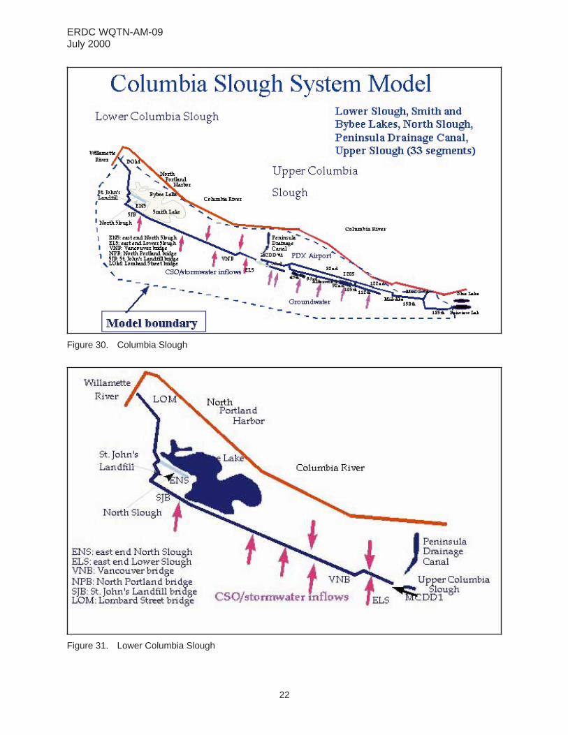
Figure 30. Columbia Slough
Figure 31. Lower Columbia Slough
ERDC WQTN-AM-09July 2000
22
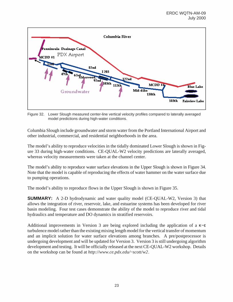
Columbia Slough include groundwater and storm water from the Portland International Airport andother industrial, commercial, and residential neighborhoods in the area.
The model’s ability to reproduce velocities in the tidally dominated Lower Slough is shown in Fig-ure 33 during high-water conditions. CE-QUAL-W2 velocity predictions are laterally averaged,whereas velocity measurements were taken at the channel center.
The model’s ability to reproduce water surface elevations in the Upper Slough is shown in Figure 34.Note that the model is capable of reproducing the effects of water hammer on the water surface dueto pumping operations.
The model’s ability to reproduce flows in the Upper Slough is shown in Figure 35.
SUMMARY: A 2-D hydrodynamic and water quality model (CE-QUAL-W2, Version 3) thatallows the integration of river, reservoir, lake, and estuarine systems has been developed for riverbasin modeling. Four test cases demonstrate the ability of the model to reproduce river and tidalhydraulics and temperature and DO dynamics in stratified reservoirs.
Additional improvements in Version 3 are being explored including the application of aκ−εturbulence model rather than the existing mixing length model for the vertical transfer of momentumand an implicit solution for water surface elevations among branches. A pre/postprocessor isundergoing development and will be updated for Version 3. Version 3 is still undergoing algorithmdevelopment and testing. It will be officially released at the next CE-QUAL-W2 workshop. Detailson the workshop can be found athttp://www.ce.pdx.edu/~scott/w2.
Figure 32. Lower Slough measured center-line vertical velocity profiles compared to laterally averagedmodel predictions during high-water conditions.
ERDC WQTN-AM-09July 2000
23

Figure 33. Columbia Slough computed versus observed water surface elevations
Figure 34. Upper Slough computed versus observed flows
ERDC WQTN-AM-09July 2000
24

POINTS OF CONTACT: This technical note was written by Dr. Scott Wells, Portland StateUniversity, and Dr. Thomas Cole, U.S. Army Engineer Research and Development Center. Foradditional Information, contact Dr. Cole (601-634-3283,[email protected]) or the Managers ofthe Water Quality Research Program, Dr. John Barko (601-634-3654,[email protected]) andMr. Robert C. Gunkel (601-634-3722,[email protected]). This technical note should be citedas follows:
Wells, S. A., and Cole, T. M. (2000). “CE-QUAL-W2, Version 3,”Water QualityTechnical Notes Collection(ERDC WQTN-AM-09), U.S. Army Engineer Research andDevelopment Center, Vicksburg, MS.www.wes.army.mil/el/elpubs/wqtncont.html
Figure 35. Upper Slough computed versus observed flows
ERDC WQTN-AM-09July 2000
25
REFERENCES
Ambrose, R. B., Wool, T., Connolly, J. P., and Schanz, R. W. (1988). “WASP4, a hydrodynamic and water qualitymodel: Model theory, user’s manual, and programmer’s guide,” Envir. Res. Lab., EPA 600/3-87/039, Athens, GA.
Berger, C., and Wells, S. (1999). “Hydraulic and water quality modeling of the Columbia Slough, Volume 1: Modeldescription, geometry, and forcing functions,” Dept. of Civil Engr., Tech. Rpt. EWR-2-99, Port. St. Univ., Portland,OR.
Cole, T., and Buchak, E. (1995). “CE-QUAL-W2: A two-dimensional, laterally averaged, hydrodynamic and waterquality model, Version 2.0,” Instruction Report EL-95-1, U.S. Army Engineer Waterways Experiment Station,Vicksburg, MS.
Donigian, A. S., Jr., Imhoff, J. C., Bicknell, B. R., and Kittle, J.L., Jr. (1984). “Application guide for hydrologicalsimulation program Fortran (HSPF),” EPA-600/3-84-065, U.S. Environmental Protection Agency, Athens, GA.
Environmental Laboratory. (1995). “CE-QUAL-RIV1: A dynamic, one-dimensional (longitudinal) water qualitymodel for streams: User’s manual,” Instruction Report EL-95-2, U.S. Army Engineer Waterways ExperimentStation, Vicksburg, MS.
Smith, D. J. (1978). “WQRRS, Generalized computer program for river-reservoir systems,” USACE Hydrol. Engr.Center, Davis, CA.
Wells, S. A. (1999). “River basin modeling using CE-QUAL-W2 Version 3.”Proc. ASCE Inter.Water Res. Engr. Conf.,Seattle, WA.
Wells, S. A. (1997). “Theoretical basis for the CE-QUAL-W2 river basin model,” Dept. of Civil Engr., Tech. Rpt.EWR-6-97, Portland St. Univ., Portland, OR.
NOTE: The contents of this technical note are not to be used for advertising, publication,or promotional purposes. Citation of trade names does not constitute an official endorse-ment or approval of the use of such products.
ERDC WQTN-AM-09July 2000
26


![· 178 w2~uz− 179 w2~− 182 w2¶a 183 w2,v0 185 w2fl 186 w2,´‡ 187 w2,^M 188 w2,â 190 w2,˛− 195 w2,ðg− 196 w2,ðg! 198 w2,ð¾ 200 w2,ð−a 201 w2,ðgG Ž ]* Z˜ ß9ü](https://img.dokumen.tips/doc/110x75/5ec4169f9cf111271f3cdc4b/178-w2uza-179-w2a-182-w2a-183-w2v0-185-w2i-186-w2a-187-w2m-188.jpg)


![[Unlocked]2 Engineer Wale (ways Experi1ttetlL Station ( WES ) ICE-QUAL-W2j CWQUA1>W2 WORKING REPORT 023 REPORT CALS CALS CALS XML 7— Title [Unlocked]](https://img.dokumen.tips/doc/110x75/60eab5e1d284cc7d816c9464/unlocked-2-engineer-wale-ways-experi1ttetll-station-wes-ice-qual-w2j-cwqua1w2.jpg)